Prediction of Peak Path of Building Carbon Emissions Based on the STIRPAT Model: A Case Study of Guangzhou City

Abstract

Carbon emissions from the building sector have a substantial effect on peak carbon targets. However, there are large differences in the carbon peak paths between different regions and buildings. This study used the stochastic impacts by regression on population, affluence, and technology (STIRPAT) model to study the peak carbon emission paths of buildings in Guangzhou City. Through ridge regression and F-tests, the main driving factors affecting carbon emissions from buildings were identified. Finally, the decreasing rate of carbon emissions per unit of building area in Guangzhou was changed to predict the time of the carbon peak. The results of the ridge regression analysis and F-test show that the urbanization rate, total floor area, consumption level of residents, value-added of the tertiary industry, and carbon emissions per unit of public floor area are the main driving factors of the model. The minimum reduction rate of carbon emissions per unit floor area required to achieve a building carbon peak in Guangzhou City by 2030 is 5%. This study provides a theoretical reference for Guangzhou to realize peak building carbon emissions.

1. Introduction

With rapid economic development, energy consumption has increased. The resulting increase in carbon emissions has exacerbated climate warming and threatened the living environment, which is an important factor restricting sustainable development in China [1,2,3,4,5]. At the Copenhagen Climate Conference, the Chinese government proposed an emission reduction target of 40% to 45% in carbon dioxide (CO₂) emissions per unit of GDP in 2020 compared to 2005 [6,7]. The Thirteenth Five-Year Plan for Energy Conservation and Carbon Reduction in Guangzhou (2016–2020) also has stated that China plans to reach peak CO₂ emissions around 2030 and will endeavor to reach its peak at an early date [8]. As a national central city and a national pilot low-carbon city, Guangzhou is striving to achieve peak total carbon emissions and must urgently explore the path of gradual decline in total carbon emissions while maintaining economic and social development.

In recent years, with increasing living standards and the rapid development of tertiary industry, carbon emissions caused by building energy consumption have been growing and becoming increasingly significant [9,10,11]. To achieve an early peak in carbon emissions and identify a pathway to accomplish it for buildings, it is crucial to identify the main driving factors of building carbon emissions and quantitatively analyze their impact on building carbon emissions, thereby predicting and studying the future trends of building carbon emissions [12,13,14].

To determine the pathways to peak building carbon emissions, it is necessary to first ascertain the main driving factors and conduct a quantitative analysis to determine their degree of influence on building carbon emissions [15,16,17]. Nord et al. [18] developed a method for modeling energy pathways for future Norwegian residential buildings by analyzing different energy supply systems. Their study showed that the implementation of stricter construction regulations had a positive impact on CO₂ emissions, while energy sources could reduce CO₂ emissions to a greater extent. Based on the extended STIRPAT model, Sun et al. [19] identified the main drivers behind carbon emissions and predicted the future emission trajectories of the ‘Belt and Road Initiative’ countries under different socio-economic pathways. Their research indicated that GDP per capita, energy consumption structure, and population were the main drivers promoting carbon emissions, while the increase in energy intensity was the main driver suppressing carbon emissions. Chen et al. [20] first employed the generalized Divisia index method to explore the factors influencing carbon emissions and to obtain the decarbonization performance of commercial building operations in 16 countries during the period of 2000–2019. The study showed that the value added by the service industry and GDP in most countries had a positive impact, while the carbon emissions per unit of value added by the service industry and carbon emissions per unit of GDP had a negative impact. Rokhmawati et al. [21] developed a systematic dynamic prediction model based on the STIRPAT model to predict the future peak of carbon emissions in Indonesia under different carbon taxes. The results showed that there was an inverse U-shaped curve between GDP per capita and CO₂ emissions, and the fastest CO₂ emission peak was expected to occur in 2040.

Existing studies on predicting future CO₂ emissions have been conducted based on various methods in China. For instance, Guo et al. [22] established a bottom-up National Energy Technology model (NET-Building) for the construction industry to depict the evolution trajectory of energy consumption and CO₂ emissions in China’s construction industry by considering the uncertainty of the future evolution trend of key variables affecting energy consumption and CO₂ emissions. The results of the study indicate that China’s building energy consumption and CO₂ emissions will peak in 2025–2040 and 2025–2035. Ma et al. [23] proposed a method for historical carbon emission assessment and a dynamic emission scenario analysis to establish a roadmap for low-carbon development in China’s residential building industry by 2050. They employed a Monte Carlo dynamic scenario simulation analysis to predict energy and emissions scenarios up to 2050. Xiang et al. [24] modeled carbon emissions from commercial buildings and used the STIRPAT model combined with LASSO regression analysis to predict that China’s carbon emissions from commercial buildings will peak by 2030, with an estimated peak emission of 126 million tons of CO₂. You et al. [25] used simulation models to forecast the peak and reduction trends in building carbon emissions under different scenarios in China. The results indicate that the Chinese building industry requires more robust strategies to achieve its peak emission targets. Li et al. [26] estimated the CO₂ emissions of China’s provincial-level building industry and calculated the Theil index of the per capita CO₂ emissions for different building types. Based on these indicators, they also used the Kaya identity to analyze the driving factors of CO₂ emission inequality in China. The results show that there is a notable inequality in emissions among different building types.

Considering the emission disparities between regions and cities, scholars have researched the peak control of carbon emissions from buildings at the provincial and municipal levels based on their respective characteristics. Huo et al. [27,28] used system dynamics and Low Emission Analysis Platform (LEAP) models to predict the peak carbon emissions in residential buildings in Chongqing, China. The results show that the carbon emissions in Chongqing may reach 2.28 billion tons (±800 million tons) by 2042, far exceeding China’s target for 2030, although different building end-uses exhibit significant differences. Jiang et al. [29] simulated Shenzhen using the LEAP model, and the results indicate that carbon emissions from the building industry in Shenzhen will peak from 2022 to 2025, with an expected decrease of >60% in CO₂ emissions by 2030. Chen et al. [30] explored the relationship between building energy consumption and socioeconomic variables using statistical data. The results indicate that carbon emissions from the building industry will peak by 2025 by adopting more electricity and renewable energy to replace coal and natural gas (NG), which are currently the main sources of heating and cooking energy.

This study employed the STIRPAT model to investigate the pathways to peak building carbon emissions in Guangzhou. By conducting a ridge regression analysis and an F-test, the main driving factors of building carbon emissions were identified, and it was determined that the minimum rate of decline per unit building area carbon emissions required to achieve peak building carbon emissions by 2030 in Guangzhou is 5%. This study provides a theoretical reference for Guangzhou to achieve its goal of achieving peak building carbon emissions.

2. Methods and Data

The flowchart of the methodology used in this study is presented in Figure 1. First, the impact factors of the STIRPAT model were identified and the parameters of the STIRPAT model were determined. The details are shown in Section 2.2. Second, in order to fit the prediction model, the multicollinearity test for each parameter in the model was carried out to determine whether each independent variable was linearly correlated. Thirdly, the ridge regression was used to fit each parameter to deal with multicollinearity parameters. Then, the F-test was utilized to verify the ridge regression. This is because the F-test is designed to test whether three or more independent variables have a significant effect on the dependent variable. Finally, the data from the Guangzhou Statistical Yearbook were used to verify the established model, and then the model simulation was carried out and the simulation results were evaluated.

2.1. Mathematical Model

This study used the STIRPAT model to study the paths of building carbon emission peaks in Guangzhou. The STIRPAT model is a stochastic regression influence model proposed by York et al. [31] based on the classic IPAT equation, I = IPAT, that is, the random influence model of population, affluence, and technology. It is expressed as follows:

$$I=a\times P^b\times A^c\times T^d\times e$$

(1)

where I is the environmental pressure; P is the population; A is the affluence; T is the technology; a is the coefficient of the model; b, c, and d are the influence indices of the corresponding driving factors; and e is the error of the model. The STIRPAT model allows the proper decomposition of each influencing factor, thus compensating for the lack of a quantitative analysis of the impact of each factor on the environment [32].

2.2. Qualitative Analysis of Influencing Factors of Building Carbon Emissions in Guangzhou

2.2.1. Total Resident Population

First, an increase in the total population will increase living energy, leading to an increase in the carbon emissions of residential buildings. Second, the greater the population, the greater the energy consumption of office buildings (such as air conditioning in offices), hotel energy consumption (such as hot water and cooking energy), hospital energy consumption (such as medical equipment energy), and other public buildings, and the more CO₂ emissions will be generated.

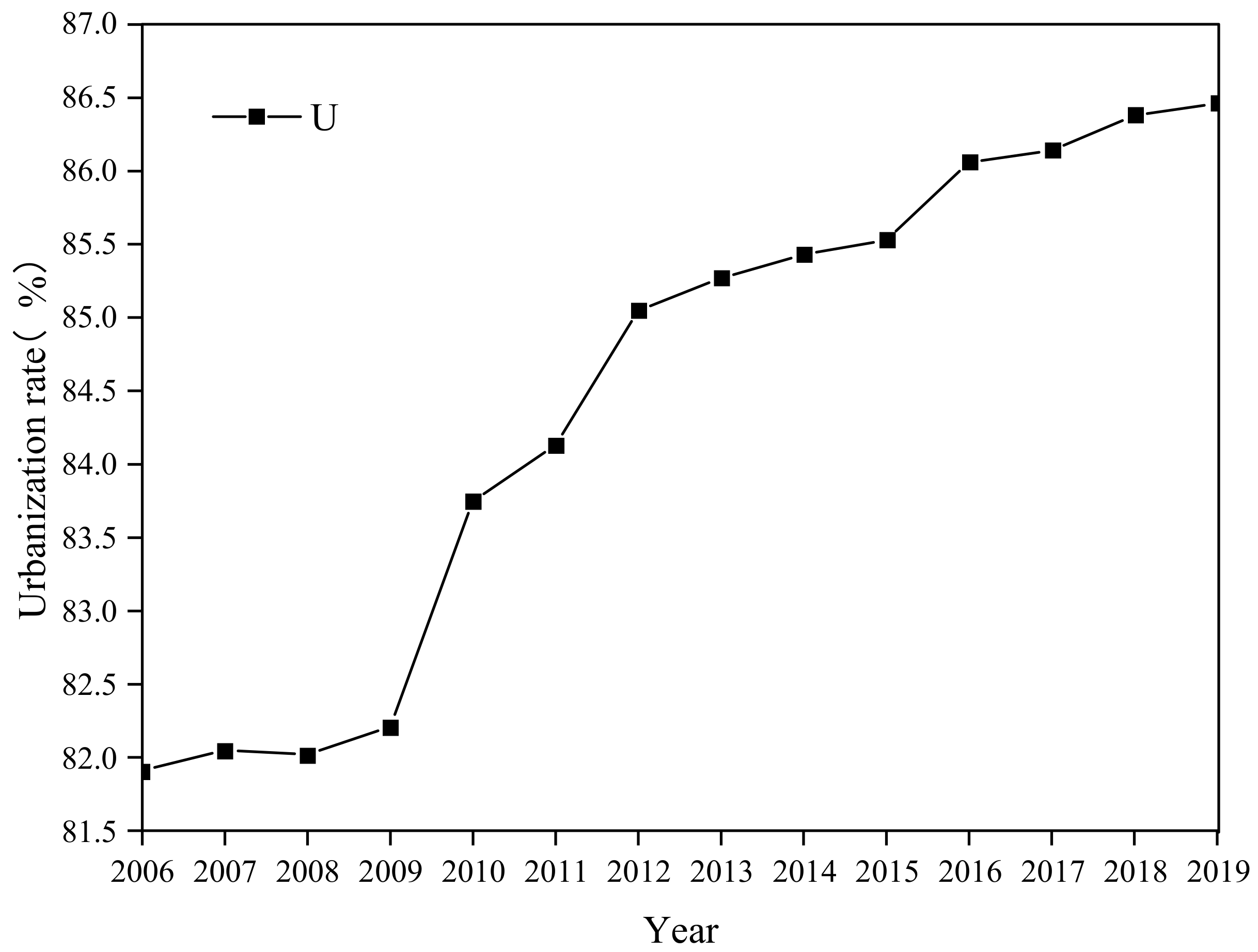
2.2.2. Urbanization Rate

The difference between the direct and indirect energy demands of urban and rural residents is an important reason for the increase in CO₂ emissions caused by an increase in the urbanization rate. Urban residents consume more energy per capita than rural residents do, and as rural residents move to cities in large numbers, CO₂ emissions increase. Urbanization leads to an increase in building land and causes the heat island effect, which increases the temperature of buildings, leading to an increase in building energy consumption and carbon emissions. Elnahls et al. [33] built a typical architectural complex in Adelaide and conducted experiments and simulations. The results showed that the average air temperatures in winter and summer were higher than meteorological temperatures. For air-conditioning systems, the energy consumption is reduced by 10% when heating the room and increases by 15% when cooling.

2.2.3. Total Building Area

The growth in the total floor area is the most direct factor causing an increase in total carbon emissions from buildings. Technically, the most important factor to consider in the design of various energy loads in a building operation process is the building area. The larger the area, the larger the energy load and the greater the resulting carbon emissions.

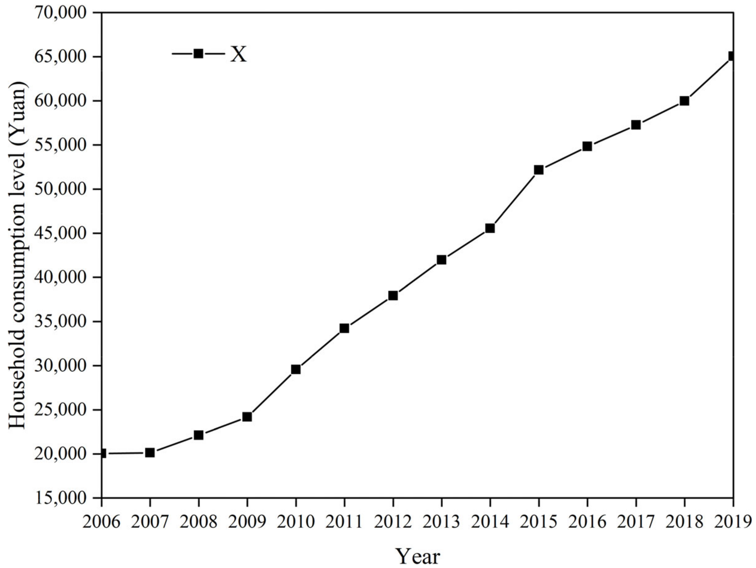
2.2.4. Residents’ Consumption Level

The level of resident consumption reflects an improvement in their living standards. With improving living standards, residents’ requirements for the comfort of buildings are also increasing, and the holding of high-energy consumption equipment, such as air conditioners, water heaters, and refrigerators, is also increasing; the frequency and duration of use is also increasing, which leads to an increase in building energy consumption, thereby increasing building carbon emissions.

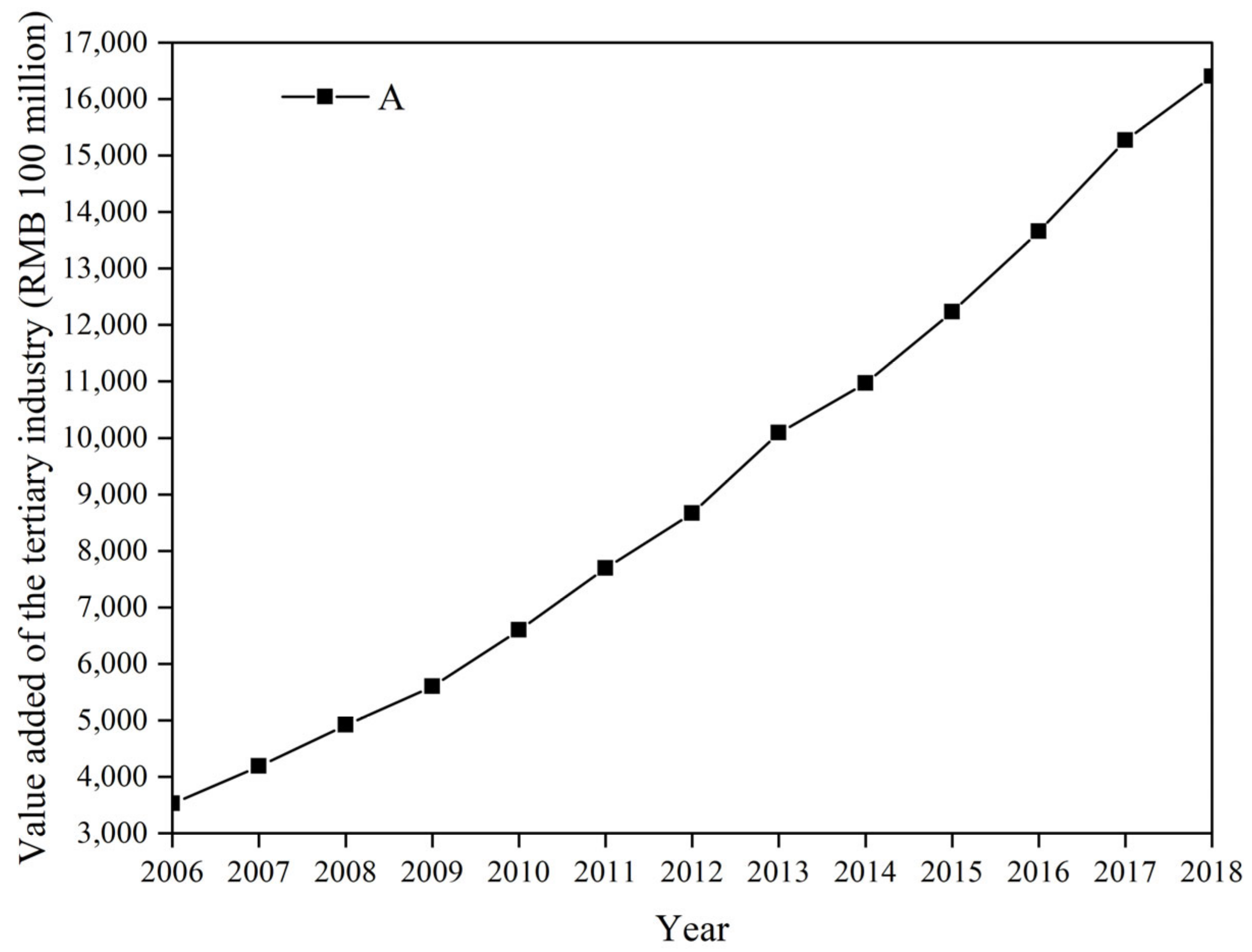
2.2.5. Added Value of the Tertiary Industry

Tertiary industries mainly comprise transportation and service industries. In recent years, with the continuous optimization of the industrial structure, the proportion of tertiary industries has increased, and the service industry has been developing rapidly. The energy consumption of the service industry occurs in public buildings, and the rapid development of the service industry will increase its energy consumption. That is, the energy consumption of public buildings will continue to increase, and the carbon emissions of public buildings will also continue to increase.

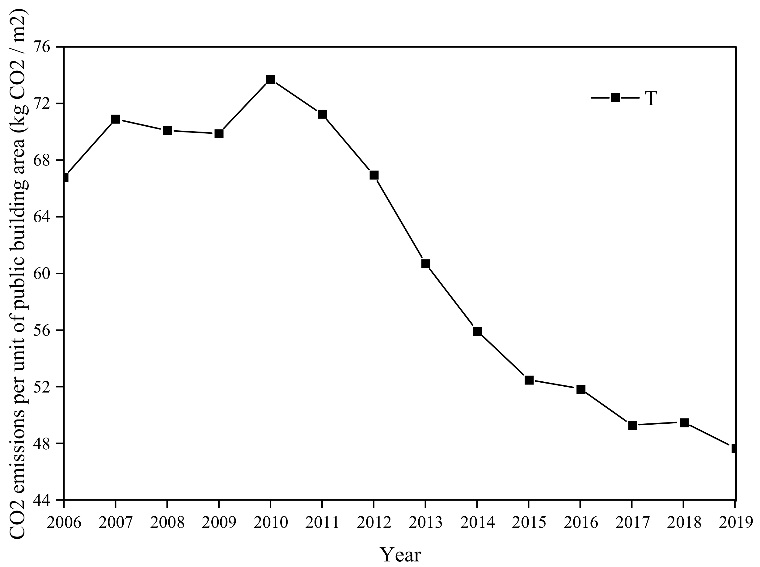
2.2.6. CO₂ Emissions per Unit of Public Building Area

Energy consumption per unit area is an important indicator of the level of energy-saving technology. According to the existing building energy consumption structure in Guangzhou, the use of clean energy such as solar energy is not popular; therefore, the energy consumption index per unit area can be equivalent to the CO₂ emissions per unit area. Although the total floor area of public buildings is smaller than that of residential buildings, the energy consumption per unit area of public buildings is approximately five times that of residential buildings. Moreover, the cost of energy consumption of residential buildings is borne by residents, whereas the cost of energy consumption of public buildings is not borne by individuals, which also leads to energy wastage and an increase in carbon emissions in public buildings. However, this shows that public buildings have considerable potential for emissions reduction. Energy conservation and emission reduction of public buildings play an important role in achieving peak building carbon emissions in Guangzhou as soon as possible.

Based on the above analysis, the permanent resident population, urbanization rate, total floor area, resident consumption level, added value of tertiary industry, and CO₂ emissions per unit of public building area were selected as the indicators affecting total building carbon emissions in Guangzhou. The total resident population and urbanization rate correspond to the population driving factors. The total construction area, consumption level, and added value of tertiary industries correspond to the driving factors of affluence. CO₂ emissions per unit of public building area correspond to technological drivers. Based on the STIRPAT model, we obtain:

$$I=K\times P^{{\alpha }_1}\times U^{{\alpha }_2}\times M^{{\alpha }_3}\times X^{{\alpha }_4}\times A^{{\alpha }_5}\times T^{{\alpha }_6}\times \epsilon$$

(2)

Taking the logarithm of both sides of the above formula yields:

$$\mathit{ln}I=\mathit{ln}K+{\alpha }_1\mathit{ln}P+{\alpha }_2\mathit{ln}U+{\alpha }_3\mathit{ln}M+{\alpha }_4\mathit{ln}X+{\alpha }_5\mathit{ln}A+{\alpha }_6\mathit{ln}T+ln\epsilon$$

(3)

Specific model variables in the formula are shown in

Table 1. Description of each variable in the model.

Variable	Instructions	Unit
I	Total building CO2 emissions	Ten thousand tons
K	Regression parameter	/
P	Permanent population	Ten thousand people
U	Urbanization	%
M	Total building area	Ten thousand square meters
X	Residents’ consumption level	Yuan
A	Added value of the tertiary industry	Hundred million yuan
T	Carbon emissions per unit of public building area	kg CO2/m2

:

2.3. Data Source and Processing

All the data used in the STIRPAT model were obtained from the Guangzhou Statistical Yearbook. Owing to the deviation in energy consumption data before 2013, this study made adjustments according to the relevant data provided by the Bureau of Statistics.

2.3.1. Population

Considering that the per-capita data of the statistical yearbook were calculated using the permanent population, this study selected the permanent population for analysis and research.

2.3.2. Area

Because the data of “actual residential floor area at the end of the year” in the statistical yearbook did not count all residential buildings, the data are too small. The total residential floor area data in this study were the average residential floor area per person multiplied by the permanent population (where the average per capita residential floor area is equal to the average per capita living area multiplied by the actual residential floor area at the end of the year divided by the actual residential living area at the end of the year). The public building area was calculated using the actual building area at the end of the year; that is, the actual residential building area at the end of the year.

2.3.3. Wealth

This study calculated resident consumption levels based on the comparable price growth rate in 2006, excluding the impact of inflation on prices.

2.3.4. Energy Consumption and Carbon Emissions

The carbon emissions of the residential buildings were calculated using the carbon emissions of domestic energy from the Guangzhou Statistical Yearbook, in which domestic energy was calculated using domestic electricity, residential liquefied petroleum gas, residential NG, and residential artificial gas. The data presented in this section are accurate and cannot be adjusted. The artificial gas used in Guangdong was mainly heavy oil-cracked gas, with a marking coefficient of 6.143 tce/10,000 m³.

The discount coefficient of electricity for each year was calculated as the ratio of electricity consumption (10,000 tons of standard coal) in the Comprehensive Energy Balance Table of the statistical yearbook to the city’s electricity consumption (10,000 kWh). Among them, the power consumption in the Comprehensive Energy Balance Table from 2006 to 2009 is the equivalent value; therefore, the nearest power discount coefficient in 2010 was used for the calculation.

The top-down method was used to calculate the energy consumption of public buildings. It was proposed that the electricity consumption of transportation accounts for 80% of the electricity consumption of transportation, warehousing, and postal services, according to which the electricity consumption of transportation is calculated. The power consumption of the service industry (i.e., the power consumption of public buildings) is equal to the power consumption of the tertiary industry minus the power consumption of traffic, according to which the power consumption of public buildings is calculated. Based on experience, the electricity consumption of public buildings accounts for approximately 90% of the total energy consumption, according to which the total energy consumption of public buildings is calculated.

In calculating the carbon emissions of public buildings based on the energy audit data of several public buildings, the ratios of fuel consumption and gas consumption to total energy consumption were proposed to be 3% and 7%, respectively.

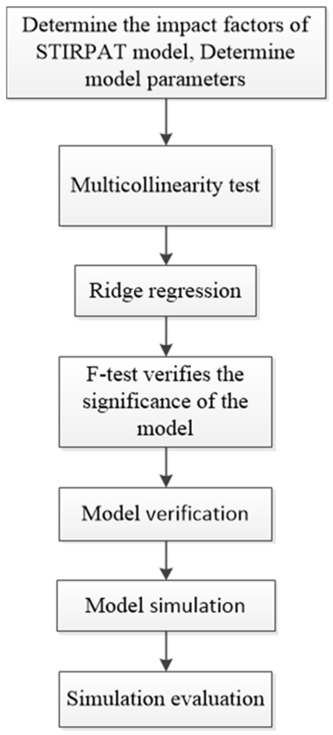
3. Model Fitting and Analysis

To determine the main driving factors of the model, this study first used multiple offline tests to determine the regression method, determined by ridge regression and regression fitting of each model parameter. Then, an F-test was conducted to determine the main driving factors of the regression model.

3.1. Multicollinearity Test

Multicollinearity refers to the phenomenon that two or more predictor variables (e.g., P, U, M, X, A, and T in Equation (4)) are highly correlated in a multiple regression model. The absence of multicollinearity could cause incorrect relationships between the independent variable (i.e., I in Equation (4)) and predictor variables. In contrast, a multicollinearity test is used to determine whether the independent variables of the model are linearly correlated [13]. To select a suitable regression method and make the regression results more reliable, a multicollinearity test among the variables was conducted before the regression analysis. The test results are listed in

Table 2. Collinearity statistics of variables (VIF).

Variables	Collinear Statistics (VIF)
P	23.081
U	23.732
M	10,173.485
X	3454.775
A	3278.469
T	1.685

.

Multicollinearity between variables increases the variance and decreases the stability of the parameter estimates. The variance inflation factor method is generally used to determine the multicollinearity of variables.

The variance inflation factor (VIF) is calculated as follows:

$${VIF}_i={(1-R_i^2)}^{-1}$$

(4)

where ${R_i}^2$ is the complex determination coefficient of the regression to other independent variables when $x_i$ is the dependent variable. The larger the variance inflation factor, the stronger the collinearity. It is believed that if the VIF exceeds 10, strong multicollinearity exists, which affects the estimate. As shown in Table 2, there is severe multicollinearity among the independent variables, except for T. The ridge regression method was used to fit the model to overcome the multicollinearity between the independent variables.

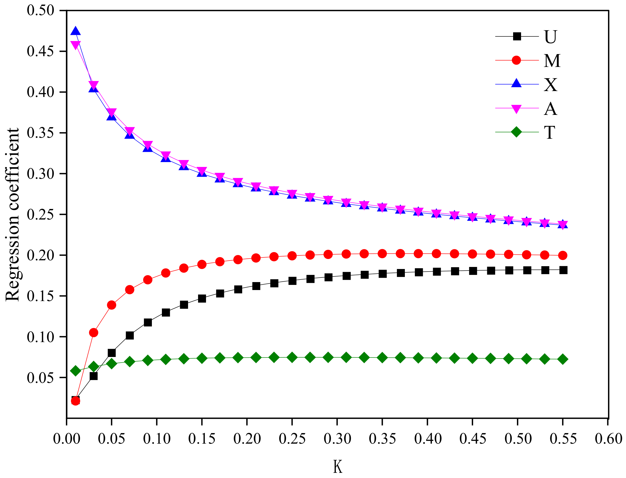
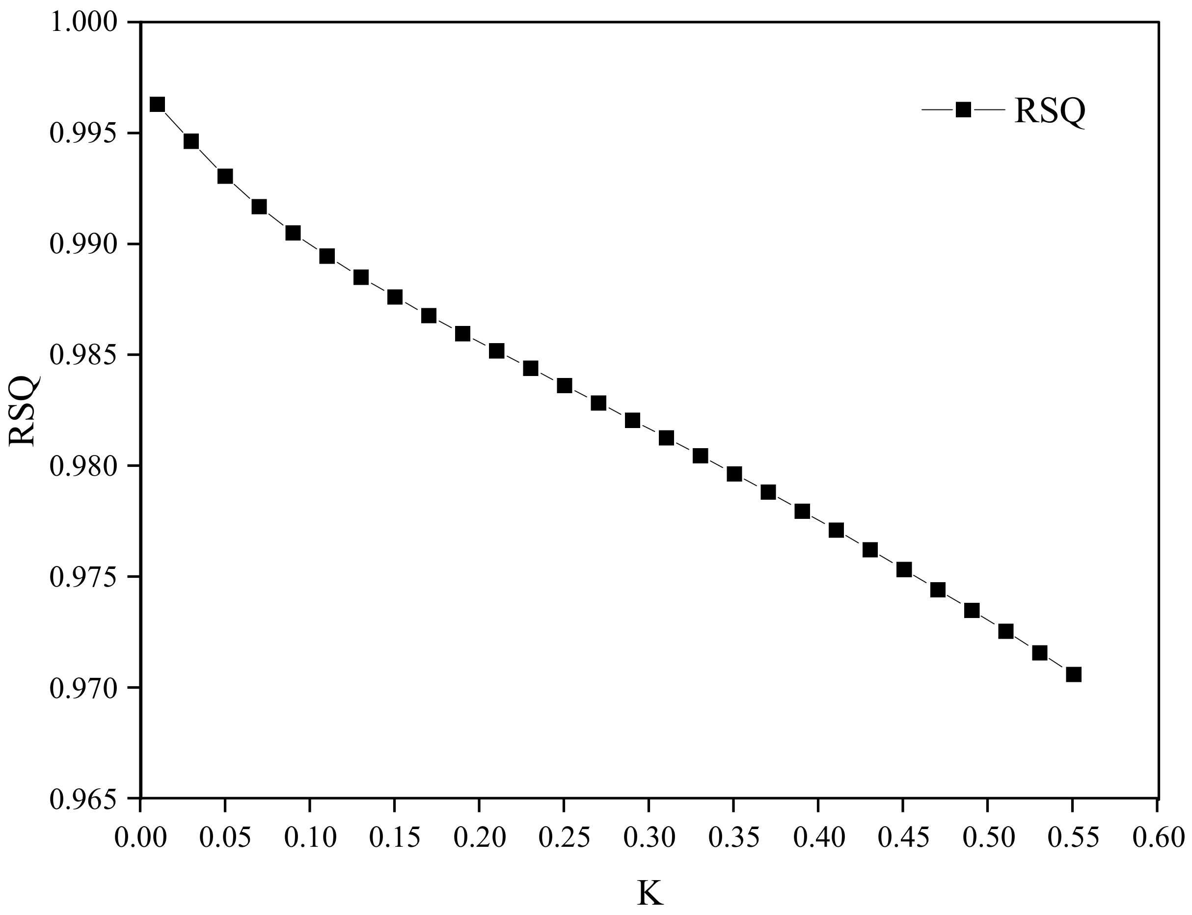
3.2. Ridge Regression Fitting

There are several strategies (e.g., ridge regression and lasso regression) to solve the problem of multicollinearity. Ridge regression was employed in this work because it is very common without considering feature selection [13]. Ridge regression is a method of regularization used to address linear regression problems. It is essentially a modified least squares method. It sacrifices the unbiased nature of the least squares method to solve the problem of multicollinearity and overfitting at the cost of losing some of the information and reducing the accuracy. Penalizing the model coefficients prevents the model from being overly complex and thus improves the robustness and generalization capability of the model [34].

The first ridge regression plot and correlation coefficient variation diagram are shown in Figure 2 and Figure 3, respectively. Figure 2 shows that when K ≥ 0.05, the regression coefficients of all variables tend to stabilize, and when K ≥ 0.08, the regression coefficients of all variables are positive. According to the value principle of K, this study selected K = 0.08 for regression. According to Figure 3, the determinability coefficient of the regression model is 0.991, indicating a high degree of goodness of fit.

The results of the ridge regression are presented in

Table 3. Results of the first ridge regression.

	B	SE(B)	Beta	B/SE(B)
P	0.0038	0.2066	0.0025	0.0186
U	1.3437	1.6667	0.1099	0.8062
M	0.1766	0.0341	0.1629	5.1730
X	0.2383	0.0594	0.3377	4.0137
A	0.2219	0.0575	0.3442	3.8579
T	0.5445	0.7039	0.0702	0.7735
Constant	−7.0109	7.1460	0.0000	−0.9811

, and the F-test results of the regression model are presented in

Table 4. First ridge regression F-test.

F Value	Sig. F	Mult. R	RSQ	Adj. RSQ	SE
18.4006	0.1766	0.9955	0.9910	0.9372	0.0486

. Table 4 shows that the significance of Sig F of the model is 0.1766, which is >0.05. This indicates that the model obtained by regression with permanent population, urbanization rate, total building area, residents’ consumption level, added value of the tertiary industry, and CO₂ emissions per unit of public building area as independent variables and total building CO₂ emissions as the dependent variable are not significant.

When the regression model was not significant, we searched for the independent variable with the smallest impact on the dependent variable according to Table 3. Through comparison, it was found that the standard regression coefficient of “permanent population” was only 0.0025, which is the smallest among all independent variables. Therefore, the independent variable “permanent population” was removed and ridge regression was conducted.

The second ridge regression plot and correlation coefficient variation diagram are shown in Figure 4 and Figure 5, respectively. Figure 4 shows that when K ≥ 0.03, the regression coefficients of all variables are positive and stable. This study selected K = 0.03 for regression. As shown in Figure 5, the determinability coefficient of the regression model is 0.995, indicating a high degree of goodness of fit.

The results of the second ridge regression are presented in

Table 5. Second ridge regression results.

	B	SE (B)	Beta	B/SE (B)
U	0.6405	1.4761	0.0524	0.4339
M	0.1138	0.1246	0.1050	0.9136
X	0.2847	0.0485	0.4035	5.8695
A	0.2641	0.0515	0.4096	5.1286
T	0.4922	0.4100	0.0635	1.2005
Constant	−3.8067	6.1148	0.0000	−0.6225

, and the F-test results are presented in

Table 6. Second ridge regression F-test.

F Value	Sig. F	Mult. R	RSQ	Adj. RSQ	SE
74.0674	0.0134	0.9973	0.9946	0.9812	0.0266

. Table 6 shows that the significance of Sig. F of the model is 0.0134, which is <0.05. The model passed the significance test, and the regression coefficients were economically significant.

The regression model for the total carbon emissions from residential buildings in Guangzhou was obtained as follows:

$$\mathit{ln}I=0.6405\mathit{ln}U+0.1138\mathit{ln}M+0.2847\mathit{ln}X+0.2641\mathit{ln}A+ 0.4922\mathit{ln}T-3.8067$$

(5)

The actual value of ln ${\mathrm{E}}_z$ was compared with the fitted value obtained from model (5) to obtain Figure 6. It can be seen that the model fits well. According to the regression results after model standardization, it can be concluded that the added value of the tertiary industry in Guangzhou has the greatest impact on the total carbon emissions of buildings, with an elasticity coefficient of 0.4096, followed by the level of household consumption, with an elasticity coefficient of 0.4035. The impacts of urbanization rate and carbon emissions per unit of public building area were relatively small, with values of 0.0524 and 0.0635, respectively.

3.3. Regression Results Analysis

In the final regression results, the permanent resident population was not included in the model because of its small impact on building carbon emissions. This may be because the urbanization rate impacts building carbon emissions in multiple aspects compared to the total population, which has become limited with the advent of family planning and changing perceptions in recent years.

Residents’ consumption levels positively impact building carbon emissions, that is, as living standards improve, building carbon emissions will continuously increase. Although the elasticity coefficient of the residents’ consumption level is large, building carbon emissions cannot be reduced at the expense of the residents’ quality of life. However, methods such as promoting a low-carbon, energy-saving lifestyle can be used to change people’s awareness of energy use, thereby reducing the impact of residents’ consumption levels on building carbon emissions.

The added value of the tertiary industry also positively impacts building carbon emissions and has the greatest impact on building carbon emissions because the energy consumption of the tertiary industry is the main component of public building energy consumption, and the tertiary industry of Guangzhou has been developing rapidly in recent years. To reduce the carbon emissions of public buildings, the development of the tertiary industry should not be promoted without control. It should develop moderately to control and reduce the excessive energy consumption caused by the economic scale effect of the tertiary industry.

Although the impact of carbon emissions per unit of public building area on the total building carbon emissions is relatively small, at only 0.0635, technological progress plays a driving role in achieving the peak of building carbon emissions. It is almost impossible for other factors, such as “urbanization rate”, “total building area”, “consumption level”, and “value added of tertiary industry” to have negative growth, and “carbon emission per unit of public building area”, as the only factor that can have negative growth, is the starting point for achieving the peak of building carbon emissions as soon as possible.

4. Quantitative Analysis of Model Driving Factors

The fitting results obtained from the STIRPAT model are shown in Equation (5). To predict future building carbon emissions based on the above model, it was first necessary to analyze the various driving factors in the model.

4.1. Urbanization Rate Analysis

The changes in the urbanization rate of Guangzhou in recent years are shown in Figure 7, and it is evident that the urbanization rate of Guangzhou has been growing. By calculating the average growth rate from 2006 to 2009 as 0.4%, the annual growth rate of the future urbanization rate in Guangzhou was set to 0.4%.

4.2. Total Building Area Analysis

The changes in the total building area of Guangzhou in recent years are shown in Figure 8, which shows that the total building area of Guangzhou shows a linear growth trend, according to which a linear regression was performed on the data of the total building area of Guangzhou from 2006 to 2019. The following fitting results were obtained:

$$y=2307.5x+23239$$

$$R^2=0.9844$$

(6)

4.3. Analysis of Residents’ Consumption Level

The changes in the consumption level of Guangzhou residents in recent years are shown in Figure 9, which shows that the consumption level of Guangzhou residents shows a linear growth trend, according to which a linear regression was performed on the data of the total building area of Guangzhou from 2006 to 2019. The following fitting results were obtained:

$$y=3747.2x+12252$$

$$R^2=0.9878$$

(7)

4.4. Analysis of the Added Value of the Tertiary Industry

The changes in the added value of the tertiary industry in Guangzhou in recent years are shown in Figure 10, which shows that the added value of the tertiary industry in Guangzhou shows a linear growth trend, according to which a linear regression was performed on the data of the total building area of Guangzhou from 2006 to 2018. The following fitting results were obtained:

$$y=1091.5x+1575.9$$

$$R^2=0.9873$$

(8)

4.5. Analysis of CO₂ Emissions per Unit of Public Building Area

As shown in Figure 11, there has been a change in the CO₂ emissions from public buildings in Guangzhou in recent years. Figure 10 shows that the CO₂ emissions per unit area of public buildings in Guangzhou have declined since 2010. According to the “Implementation Plan for Coal Control Targets in the Construction Sector of the 13th Five-Year Plan” released by the Coal Control Project Team of Beijing Jiaotong University, key cities should complete the renovation of 400 million m² of public buildings by 2020, achieving a reduction in energy consumption per unit area of public buildings by >20% [35]. Considering the optimization and adjustment of the energy structure of public buildings, this study calculates and analyzes the peak carbon emissions from buildings under three scenarios: 4%, 5%, and 6% annual decline rates in carbon emissions per unit area in Guangzhou.

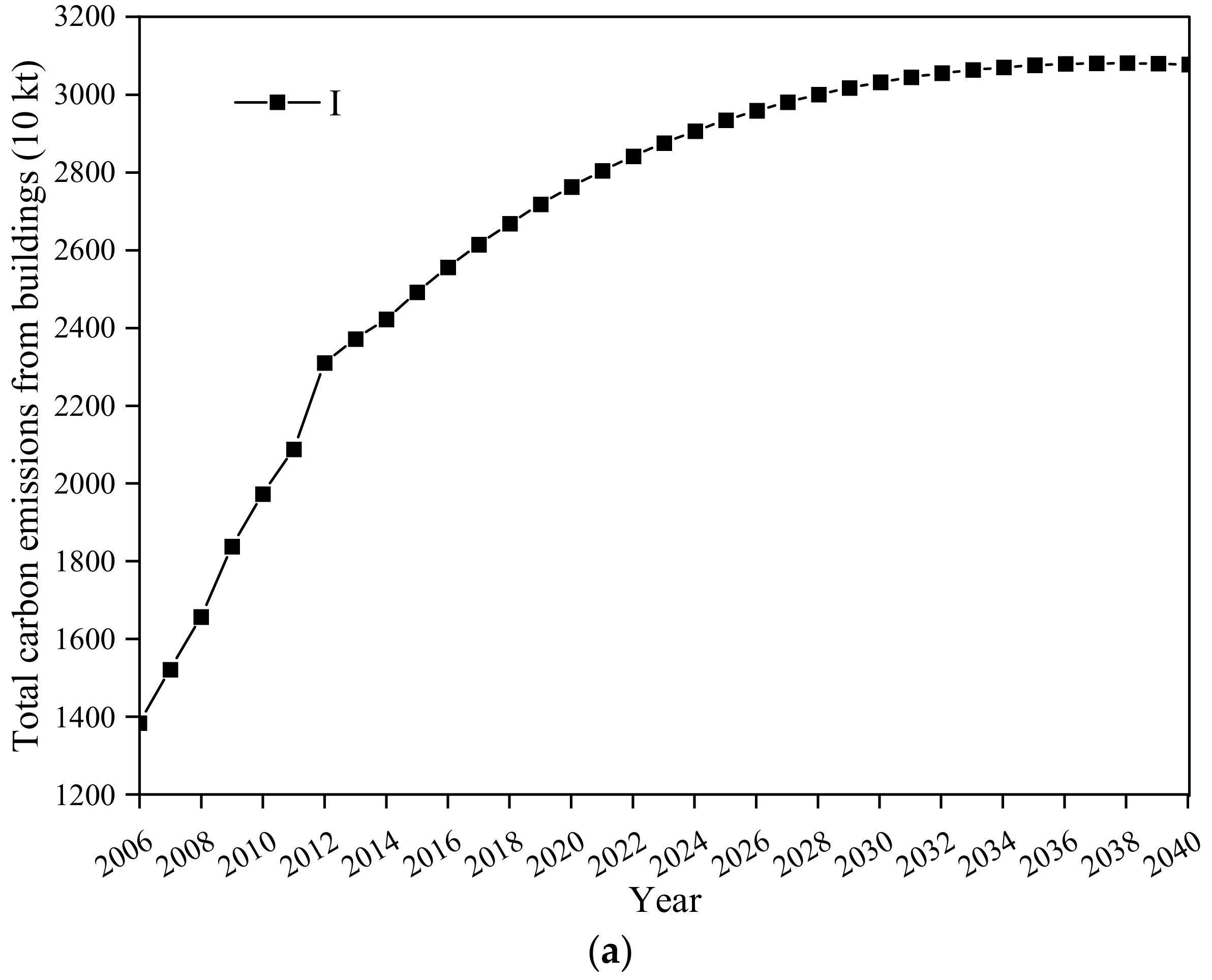
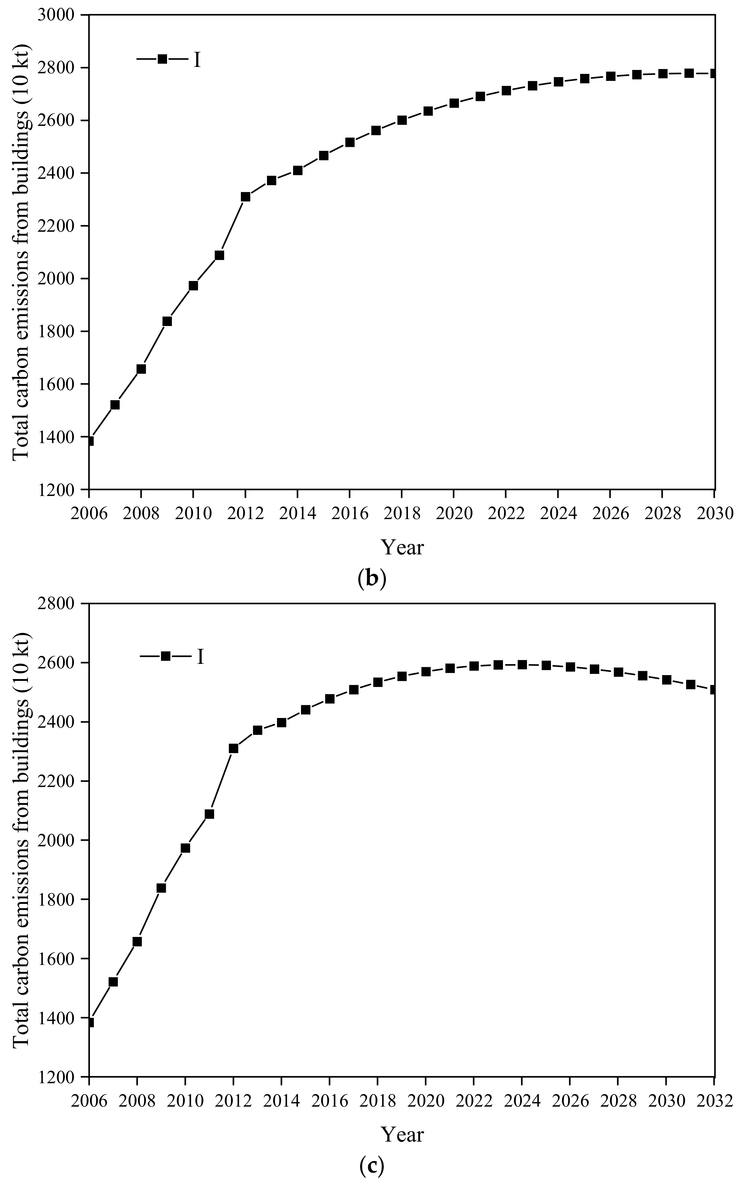
5. Prediction of Total Building Carbon Emissions in Guangzhou

The predicted values of each of the above drivers were incorporated into the matching equation of the STIRPAT model, and the annual decline rate of carbon emissions per unit of building area in Guangzhou City in the future was set to 4%. The results are shown in Figure 12a. From the results, it is evident that if the annual decline rate of carbon emissions per unit of building area in Guangzhou is set at 4% in the future, carbon emissions from buildings in Guangzhou will peak by 2038.

The consequences of setting the annual decline rate of carbon emissions per unit of building area in Guangzhou to 5% in the future are shown in Figure 12b. From the results, it can be seen that if the annual decline rate of carbon emissions per unit of building area in Guangzhou is set at 5% in the future, the carbon emissions from buildings in Guangzhou will peak in 2029.

The consequences of setting the annual decline rate of carbon emissions per unit of building area in Guangzhou to 6% in the future are shown in Figure 12c. From the results, it can be easily seen that if the annual decline rate of carbon emissions per unit of building area in Guangzhou is set at 6% in the future, the carbon emissions from buildings in Guangzhou will peak in 2024.

6. Conclusions and Policy Implications

This study investigated the peak pathway of carbon emissions from buildings in Guangzhou using the STIRPAT model. The main driving factors of Guangzhou’s building carbon emissions were quantitatively analyzed using ridge regression analysis and an F-test. Furthermore, the peak time of carbon emissions from buildings in Guangzhou was predicted under different annual carbon emission decline rates per unit area. The main conclusions of this study are as follows:

(1)

The STIRPAT model incorporates the main driving factors of the urbanization rate, total building area, resident consumption level, tertiary industry value-added, and carbon emissions per unit area of public buildings. The urbanization rate, total building area, resident consumption level, and tertiary industry value-added had a positive impact on building carbon emissions, whereas the impact of the permanent population on building carbon emissions was negligible and was not included in the model. The carbon emissions per unit area of public buildings have a minimal impact on total building carbon emissions; however, they reflect the role of technological progress in achieving peak building carbon emissions.

(2)

The minimum annual decline rate of carbon emissions per unit area for Guangzhou to achieve peak building carbon emissions by 2030 is 5%. If the rate of decline is <5%, peak carbon emissions will only be achieved after 2030.

It was evident from this paper that the urbanization rate and carbon emissions per unit area of public buildings have a great influence on the model. To achieve peak building carbon emissions in Guangzhou by 2030, the annual decline rate of carbon emissions per unit area must be at least 5%. According to the calculation, if the annual decline rate of carbon emissions per unit area is 3%, it will be impossible to achieve building carbon emissions peaking until 2050. However, the permanent population was excluded from this paper owing to its having less influence on the model. Therefore, the policy recommendations of this study for the future are as follows:

First, it is recommended to promote the development of high-quality urbanization in Guangzhou City, which is similar to the conclusion in [36].

Second, it is suggested that various types of carbon emissions during building construction and operation and maintenance should be reduced, such as implementing policies to slow down the progress of new housing construction and promote high-quality low-carbon construction. Moreover, it is beneficial to adopt environmentally friendly materials and make reasonable use of thermal insulation materials and less use of materials such as glass curtain walls in the construction of new housing.

There are some shortcomings in the research of this paper. The STIRPAT model may generate duplicate interpretations, but this study eliminated the parameters that were not significant to the model by multicollinearity testing and ridge regression and obtained the weights of each parameter’s influence on the significance of the model, which also increased the complexity of the model. With the further development of society and technology, the methods of predicting building carbon emissions will face new challenges and opportunities, and we need to continue to explore new paths to reduce emissions.

References

1. Webster, M.D.; Meryman, H.; Kestner, D.M. Carbon Emissions and Building Structure: What the Structural Engineer Needs to Know about Carbon in the 21st Century. In Structures Congress 2011; ASCE: Reston, VA, USA, 2011; pp. 472–482. [Google Scholar]
2. Atmaca, A.; Atmaca, N. Carbon footprint assessment of residential buildings, a review and a case study in Turkey. J. Clean. Prod. 2022, 340, 130691. [Google Scholar] [CrossRef]
3. Gao, H.; Wang, X.; Wu, K.; Zheng, Y.; Wang, Q.; Shi, W.; He, M. A Review of Building Carbon Emission Accounting and Prediction Models. Buildings 2023, 13, 1617. [Google Scholar] [CrossRef]
4. Cheng, J.; Mao, C.; Huang, Z.; Hong, J.; Liu, G. Implementation strategies for sustainable renewal at the neighborhood level with the goal of reducing carbon emission. Sustain. Cities Soc. 2022, 85, 104047. [Google Scholar] [CrossRef]
5. Yang, Z.; Gao, W.; Han, Q.; Qi, L.; Cui, Y.; Chen, Y. Digitalization and carbon emissions: How does digital city construction affect China’s carbon emission reduction? Sustain. Cities Soc. 2022, 87, 104201. [Google Scholar] [CrossRef]
6. Ares, E.; Bennett, O.; Bolton, P. Climate change: The Copenhagen conference. Econ. Indic. 2009, 3, 9. [Google Scholar]
7. Wang, X.; Wang, G.; Chen, T.; Zeng, Z.; Heng, C.K. Low-carbon city and its future research trends: A bibliometric analysis and systematic review. Sustain. Cities Soc. 2023, 90, 104381. [Google Scholar] [CrossRef]
8. Guangzhou Municipal People’s Government. Notice of General Office of Guangzhou Municipal People’s Government on Issuing the 13th Five-Year Plan for Energy Conservation and Carbon Reduction of Guangzhou (2016–2020); Guangzhou Municipal People’s Government Bulletin: Guangzhou, China, 2017; Volume 13, pp. 29–31. [Google Scholar]
9. Wang, G.; He, L.; Guo, J.; Huang, J. The estimation of building carbon emission using nighttime light images: A comparative study at various spatial scales. Sustain. Cities Soc. 2023, 101, 105066. [Google Scholar] [CrossRef]
10. Lu, K.; Deng, X. OpenBIM-based assessment for social cost of carbon through building life cycle. Sustain. Cities Soc. 2023, 99, 104871. [Google Scholar] [CrossRef]
11. Hashempour, N.; Taherkhani, R.; Mahdikhani, M. Energy performance optimization of existing buildings: A literature review. Sustain. Cities Soc. 2020, 54, 101967. [Google Scholar] [CrossRef]
12. Li, R.; Yu, Y.; Cai, W.; Liu, Q.; Liu, Y.; Zhou, H. Interprovincial differences in the historical peak situation of building carbon emissions in China: Causes and enlightenments. J. Environ. Manag. 2023, 332, 117347. [Google Scholar] [CrossRef] [PubMed]
13. Xu, G.; Wang, W. China’s energy consumption in construction and building sectors: An outlook to 2100. Energy 2020, 195, 117045. [Google Scholar] [CrossRef]
14. Lu, Y.; Cui, P.; Li, D. Which activities contribute most to building energy consumption in China? A hybrid LMDI decomposition analysis from year 2007 to 2015. Energy Build. 2018, 165, 259–269. [Google Scholar] [CrossRef]
15. Xiao, Y.; Huang, H.; Qian, X.-M.; Zhang, L.-Y.; An, B.-W. Can new-type urbanization reduce urban building carbon emissions? New evidence from China. Sustain. Cities Soc. 2023, 90, 104410. [Google Scholar] [CrossRef]
16. He, J.; Yue, Q.; Li, Y.; Zhao, F.; Wang, H. Driving force analysis of carbon emissions in China’s building industry: 2000–2015. Sustain. Cities Soc. 2020, 60, 102268. [Google Scholar] [CrossRef]
17. Tan, X.; Lai, H.; Gu, B.; Zeng, Y.; Li, H. Carbon emission and abatement potential outlook in China’s building sector through 2050. Energy Policy 2018, 118, 429–439. [Google Scholar] [CrossRef]
18. Nord, N.; Ding, Y.; Skrautvol, O.; Eliassen, S.F. Energy Pathways for Future Norwegian Residential Building Areas. Energies 2021, 14, 934. [Google Scholar] [CrossRef]
19. Sun, L.; Cui, H.; Ge, Q. Driving Factors and Future Prediction of Carbon Emissions in the ‘Belt and Road Initiative’ Countries. Energies 2021, 14, 5455. [Google Scholar] [CrossRef]
20. Chen, L.; Ma, M.; Xiang, X. Decarbonizing or illusion? How carbon emissions of commercial building operations change worldwide. Sustain. Cities Soc. 2023, 96, 104654. [Google Scholar] [CrossRef]
21. Rokhmawati, A.; Sarasi, V.; Berampu, L.T. Scenario analysis of the Indonesia carbon tax impact on carbon emissions using system dynamics modeling and STIRPAT model. Geogr. Sustain. 2024, 5, 577–587. [Google Scholar] [CrossRef]
22. Guo, Y.; Uhde, H.; Wen, W. Uncertainty of energy consumption and CO2 emissions in the building sector in China. Sustain. Cities Soc. 2023, 97, 104728. [Google Scholar] [CrossRef]
23. Ma, M.; Ma, X.; Cai, W.; Cai, W. Low carbon roadmap of residential building sector in China: Historical mitigation and prospective peak. Appl. Energy 2020, 273, 115247. [Google Scholar] [CrossRef]
24. Xiang, X.; Ma, X.; Ma, Z.; Ma, M. Operational Carbon Change in Commercial Buildings under the Carbon Neutral Goal: A LASSO—WOA Approach. Buildings 2022, 12, 54. [Google Scholar] [CrossRef]
25. You, K.; Ren, H.; Cai, W.; Huang, R.; Li, Y. Modeling carbon emission trend in China’s building sector to year 2060. Resour. Conserv. Recycl. 2023, 188, 106679. [Google Scholar] [CrossRef]
26. Li, H.; Qiu, P.; Wu, T. The regional disparity of per-capita CO2 emissions in China’s building sector: An analysis of macroeconomic drivers and policy implications. Energy Build. 2021, 244, 111011. [Google Scholar] [CrossRef]
27. Huo, T.; Xu, L.; Feng, W.; Cai, W.; Liu, B. Dynamic scenario simulations of carbon emission peak in China’s city-scale urban residential building sector through 2050. Energy Policy 2021, 159, 112612. [Google Scholar] [CrossRef]
28. Huo, T.; Xu, L.; Liu, B.; Cai, W.; Feng, W. China’s commercial building carbon emissions toward 2060: An integrated dynamic emission assessment model. Appl. Energy 2022, 325, 119828. [Google Scholar] [CrossRef]
29. Jiang, J.-J.; Ye, B.; Zeng, Z.-Z.; Liu, J.-G.; Yang, X. Potential and roadmap of CO2 emission reduction in urban buildings: Case study of Shenzhen. Adv. Clim. Chang. Res. 2022, 13, 587–599. [Google Scholar] [CrossRef]
30. Chen, H.; Chen, W. Carbon mitigation of China’s building sector on city-level: Pathway and policy implications by a low-carbon province case study. J. Clean. Prod. 2019, 224, 207–217. [Google Scholar] [CrossRef]
31. York, R.; Rosa, E.A.; Dietz, T. A rift in modernity? Assessing the anthropogenic sources of global climate change with the STIRPAT model. Int. J. Sociol. Soc. Policy 2003, 23, 31–51. [Google Scholar] [CrossRef]
32. York, R.; Rosa, E.A.; Dietz, T. STIRPAT, IPAT and IMPACT: Analytic tools for unpacking the driving forces of environmental impacts. Ecol. Econ. 2003, 46, 351–365. [Google Scholar] [CrossRef]
33. Elnahas, M.; Williamson, T. An improvement of the CTTC model for predicting urban air temperatures. Energy Build. 1997, 25, 41–49. [Google Scholar] [CrossRef]
34. Yang, Y.; Dong, R.; Ren, X.; Fu, M. Exploring Sustainable Planning Strategies for Carbon Emission Reduction in Beijing’s Transportation Sector: A Multi-Scenario Carbon Peak Analysis Using the Extended STIRPAT Model. Sustainability 2024, 16, 4670. [Google Scholar] [CrossRef]
35. Beijing Jiaotong University. Implementation Plan for Coal Control targets in the Construction Sector of the 13th Five-Year Plan. In Proceedings of the 4th International Symposium on Total Coal Consumption Control and Energy Transition in China, Beijing, China, 30 November 2017; China Energy Conservation Association: Beijing, China, 2017; pp. 1–44. [Google Scholar]
36. Wang, S.; Wang, J.; Li, S.; Fang, C.; Feng, K. Socioeconomic driving forces and scenario simulation of CO2 emissions for a fast-developing region in China. J. Clean. Prod. 2019, 216, 217–229. [Google Scholar] [CrossRef]
Figure 1. The flowchart of the methodology used in the study.
Energies 18 01633 g001
Figure 2. First ridge regression trace map.
Energies 18 01633 g002
Figure 3. First ridge regression correlation coefficient R2 changes in ridge regression parameter K.
Energies 18 01633 g003
Figure 4. Second ridge regression trace map.
Energies 18 01633 g004
Figure 5. Second ridge regression correlation coefficient R2 changes in ridge regression parameter K.
Energies 18 01633 g005
Figure 6. Comparison between the actual value of I and the fitted value obtained from model regression.
Energies 18 01633 g006
Figure 7. Changes in urbanization rates.
Energies 18 01633 g007
Figure 8. Changes in total building area.
Energies 18 01633 g008
Figure 9. Changes in residents’ consumption level.
Energies 18 01633 g009
Figure 10. Changes in the added value of the tertiary industry.
Energies 18 01633 g010
Figure 11. Variation in CO2 emissions per unit of public building area.
Energies 18 01633 g011
Figure 12. Variation in total carbon emissions from buildings in Guangzhou, 2006–2030 (a) ∆T = −4%, (b) ∆T = −5%, (c) ∆T = −6%.
Energies 18 01633 g012aEnergies 18 01633 g012b