Article

Heat Transfer Analysis in Double Diaphragm Preforming Process of Dry Woven Carbon Fibres

1
Aerostructures Innovation Research Hub (AIR Hub), Swinburne University of Technology, Melbourne, VIC 3122, Australia
2
Department of Mechanical Engineering and Product Design Engineering, Swinburne University of Technology, Melbourne, VIC 3122, Australia
*
Author to whom correspondence should be addressed.
Energies 2025, 18(6), 1471; https://doi.org/10.3390/en18061471
Submission received: 28 January 2025 / Revised: 24 February 2025 / Accepted: 11 March 2025 / Published: 17 March 2025
(This article belongs to the Special Issue Advanced Analysis of Heat Transfer and Energy Conversion 2024)

Abstract

:
Double diaphragm forming (DDF) represents an efficient manufacturing technique leveraging vacuum pressure and heat to form composite material stacks between flexible diaphragms. This study focuses on the critical role of thermal management during preforming, essential for material integrity, defect mitigation, and process efficiency. A comprehensive three-dimensional finite element model (FEM) is developed to investigate the heat transfer dynamics in DDF, incorporating temperature-dependent material properties such as specific heat and thermal conductivity under compaction and varying density conditions. A novel approach is introduced to predict thermal contact conductance (TCC) across multilayer carbon fabric interfaces, validated using four laminate configurations. The resulting effective thermal conductivity of the laminates is applied in production-scale simulations, enabling accurate predictions of temperature distributions, which are corroborated by experimental data. The findings highlight the significant impact of mesoscale interactions, such as yarn-level deformation and surface asperities, on TCC variation. The study provides an enhanced understanding of heat transfer mechanisms in DDF, offering insights to optimise process parameters, improve product quality, and advance manufacturing capabilities for complex geometries.

1. Introduction

Double diaphragm forming (DDF) is a cost-effective manufacturing method widely employed in liquid composite moulding (LCM) to produce high-quality unconsolidated component shapes [1]. Its scalability and suitability for diverse production volumes make it an attractive choice for manufacturing industries prioritising efficiency, automation and precision [2]. A key advantage of DDF is its uniform contact with the plies, which minimises the out-of-plane wrinkling, enhances process stability and repeatability, and enables quick demoulding [3]. Additionally, DDF supports the fabrication of near-net shapes with complex geometries, minimal material waste, high automation potential, and relatively low capital investment [4,5,6,7]. This versatile technique has been successfully employed in processing various materials, including thermoset prepregs [8], non-crimp dry fabrics (NCFs) [9], thermoplastics [10], and dry biaxial fabrics [11,12,13]. Among these materials, woven fabrics are frequently used structural applications due to their superior control over fibre displacement and improved handling and transport during LCM processing [14].
For dry woven carbon fabrics, the DDF is particularly advantageous as it maintains fibre alignment, minimises defects (e.g., wrinkling, bridging) and ensures precise conformity to mould geometries without compromising fabric integrity [15,16]. When optimised through material selection, tooling design and process control, DDF meets the stringent requirements of aerospace structural applications, delivering high-quality defect-free preforms within the LCM process chain. Furthermore, its high automation capability significantly reduces the labour costs, enhances process efficiency and ensures scalability for industrial production [1,9,11,15,16,17,18,19,20,21].
In the DDF process, the compaction behaviour of dry fabrics without binders is influenced by their woven nature, which introduces crimp into both single-ply and multilayer configurations. During the DDF process, a single ply exhibits a characteristic three-phase compaction pattern. Initially, a linear trend is observed as pressure reduces gaps between yarns and fibres. This is followed by a nonlinear phase where increased pressure leads to a further reduction in gaps within the fabric. Finally, a second linear phase occurs, driven primarily by the bending deformations of the yarns as the material becomes increasingly compact [22,23]. In multilayer fabrics without binders, the compaction process mirrors the three phases observed in single-ply fabrics but introduces an additional factor due to fabric–fabric interaction, also known as nesting. Nesting significantly contributes to thickness reduction as adjacent layers interact during compaction. This behaviour can be mathematically modelled by treating the crimped yarns in adjacent layers as sine waves, with the degree of nesting determined by the phase shift between these waves. Maximum nesting, which results in the greatest thickness reduction, occurs at dimensionless phase shift angles of ±π/2 (asymmetric superimposition), while non-nesting, which minimises thickness reduction, occurs at 0° and ±π (symmetric superimposition) [24].
The nesting and compaction behaviour can be theoretically understood and quantified by analysing changes in crimp angles between warp and weft yarns under pressure, alongside their influence on material properties [24,25,26]. This phenomenon impacts the overall structural and thermal properties of the fabric stack when it is constantly under compaction load. For instance, Zheng et al. [27] investigated the structural parameters of a twill weave glass fibre fabrics numerically, demonstrating that weave structure and increased warp density both reduce heat transfer properties, primarily due to structural variations [27]. However, post-decompaction, it is important to note that in dry fabrics cut for assembly and undergoing the DDF process, fabric edges may lose stability, leading to fraying and elastic thickness recovery. To address these challenges, specific trimming and stabilisation techniques can be employed to maintain edge stability and dimensional consistency [28].
Stabilisation techniques are crucial for producing preforms that achieve the desired volume fraction and structural integrity. By enhancing stability, these preforms can be efficiently transported and handled automatically during subsequent LCM processing steps without incurring distortion. When stabilisation is conducted under DDF conditions, it is referred to as double diaphragm preforming (DDPF). This technique involves embedding the carbon fabric plies with thermoplastic or thermoset (reactive) binders. These binders effectively tack adjacent layers, resulting in binder-stabilised preforms upon the application of heat and subsequent cooling [20,28,29,30]. The selection of binders plays a crucial role in the DDPF process, as they come in various forms, such as powders, veils, commingled yarns, hot melt webs, and adhesive films. Each type of binder distinctly influences the mechanical properties, thermophysical behaviour, and resin permeability of the preforms, allowing for optimisation of their characteristics for specific applications [31,32,33].
The incorporation of binders in DDPF significantly enhances the initial thickness of preforms, impacting their elastic and viscoelastic properties. Additionally, this inclusion establishes an inverse relationship between the compression rate during the forming process and the resulting thickness of the preform. Furthermore, the binders influence the nesting behaviour, the bending of the yarns, and the gaps arising from variations in contact between fabric layers. Studies indicate that an optimal binder content of 4 wt% strikes a crucial balance between formability and mechanical performance [30]. From a thermophysical perspective, a 4 wt% binder content reduces the rate of heat transfer through the thickness of the preform while increasing its specific heat capacity due to the introduction of gaps and additional material between the fabrics [34]. In terms of resin permeability, the location and concentration of binders are critical, as they can obstruct resin flow channels between fibre tows, thereby affecting the overall permeability of the resin system in various directions [32,35].
In the DDPF process, binder systems are activated using a variety of heating methods commonly employed in industrial applications, including infrared heaters, heated tooling, ovens, autoclaves, and inductive or ultrasonic heating devices [20,36]. Each of these methods offers distinct advantages and disadvantages based on factors such as cooling systems, cycle times, part geometry, heat transfer efficiency and overall process control [36]. A particularly effective approach in the DDPF process is the use of isothermal multi-section tooling for automated preforming, which mitigates prebonding and the formation of overheated zones that could lead to binder degradation and reduced preform quality [34,36,37]. This technique ensures uniform temperature distribution throughout the thin preform, a critical factor in achieving optimal interlayer bonding, enhancing energy efficiency, and maintaining precise process control, similar to the critical temperature control required during resin curing [37].
The DDPF process operates under complex multi-physics conditions influenced by variations in thickness, compression, friction, bending, in-plane tension, heat transfer, phase changes and boundary losses. Consequently, extensive numerical and experimental studies have been conducted across various material systems to explore these interactions [1,4,9,11,13,17,18,20,21,34]. Among these studies, to prioritise optimisation, numerical simulations are increasingly employed for effective mechanical process and defect predictions, significantly reducing reliance on costly trial-and-error experimental methodologies [3,38,39]. These mechanical simulations require accurate material characterisation models that can effectively predict defects during the numerical process simulations [21,40,41]. Similarly, thermal simulations also require precise understanding of the heat transfer properties of the preforms and bagging materials, particularly under the conditions associated with the DDPF processing conditions [34,42,43].
Current thermal characterisation techniques [44] and heat transfer studies applied to a variety of engineering materials use experimental methods [34,42,43,45,46,47,48,49,50,51], numerical simulations, and hybrid approaches combining both [52,53,54,55,56,57,58,59,60,61,62,63,64,65]. Among these, experimental methods typically include established techniques such as laser flash analysis (LFA), guarded heat flow meters, transient plane source (TPS) methods, and modified transient plane source (MTPS) methods. In addition to these standard techniques, non-standard approaches such as thermal mapping [34,43], time-domain thermoreflectance (TDTR), the 3ω method, and frequency-domain thermoreflectance (FDTR) [45] have also been utilised to provide deeper insights. In numerical studies, some approaches accurately model the interface geometry to include the surface roughness of effects, while others simplify the representation by using a virtual layer model, depending on the application requirements. By accurately replicating the temperature boundary conditions observed in experimental setups, these studies effectively predict material heat transfer properties [45,57,66]. Some investigations extend to multilayer materials, incorporating models that account for thermal contact conductance (TCC) at the interfaces [39,44,48,66,67,68,69,70,71,72]. This focus on TCC is essential, as the structural composition of woven fabrics and the varying contact interactions at interfaces influence heat flow, making the effective thermal conductivity of multilayer stacks dependent on the number of interfaces [48].
Traditional experimental methods for determining thermal conductivity often rely on parameter or function estimation through inverse heat transfer problem (IHTP) techniques but generally do not account for TCC effects across multiple stack locations. This oversight can lead to underestimation of the actual thermal conductivity [48,71,72,73,74,75]. Alternatively, surface roughness measurements have been used to predict TCC, utilising scale-resolved boundary geometries to estimate contact resistance and applying numerical methods for TCC prediction [66,67,69]. Calibration techniques for TCC and resistance estimation have also been developed for both single metallic interfaces [68] and two interfaces in a three-layer composite stack [70]. The TCC effects in thick multilayer fabric stacks, such as those used in structural aircraft components, remain largely unexplored due to the challenges involved in characterising interfacial asperities during the preforming process. In woven fabrics, nesting effects and the presence of binder at the layer interfaces further complicate the precise TCC determination, as the binder redistribution and phase change during DDPF alters the thermal resistance. Existing models often focus on lower layer stacks where the TCC effects are negligible; however, for production-scale components, these effects compound, leading to unreliable heat distribution predictions. This research gap contributes to costly manufacturing defects in critical composite structures that arise during preform, leading to uneven compaction, resin-rich zones and uneven curing.
This study addresses this gap in understanding TCC by examining four configurations (12, 24, 48 and 96 layers) at the coupon level under DDPF conditions. Experimental analysis of compaction-driven heat transfer is combined with parameter-tuned numerical modelling to establish a layer count-dependent TCC relationship. This resolves interdependencies between the binder presence, nesting and interfacial thermal resistance. The resulting framework is then tested and validated on production-scale preforms, providing a validated digital tool to optimise the heat transfer process and minimise energy losses. This enhances the accuracy of temperature predictions while informing tooling design processes in aerospace composite manufacturing.

2. Materials and Experimental Methods

2.1. Materials and Thermophysical Properties

This study utilised a 3K aerospace-grade 2 × 2 twill carbon fabric (CF), Style 452-5, supplied by Engineered Cramer Composites (ECC), Heek, Germany, as shown in Figure 1a. This carbon fabric has an aerial weight of 204 g m−2, with fibre diameters of 7 µm and a density of 1800 kg m−3. The linear density of fibres in both the weft and warp directions is 200 tex. The optical surface roughness variations in loom state are presented in Figure 1b with a highest z-direction variation of 1640.74 µm.
The binder material for preforming is Spunfab PA1203 (a co-polyamide binder) sourced from Spunfab Ltd., Cuyahoga Falls, OH, USA, embedded between two fabric layers for tacking, as shown in Figure 1a. This Spunfab PA binder has an aerial weight of 7.4 g m−2, a melt volume rate of (30–50) cm3 per 10 min, and a melting range of (85–98) °C. For the diaphragm (bagging) material used in the DDPF process, portions of a silicone diaphragm membrane (Mosites #1453-D) from Mosites Rubber Company, Fort Worth, TX, USA, are employed. This silicone membrane has a density of 1150 kg m−3, an aerial weight of 1840 g m−2 a thickness of 1.52 mm, and an operating temperature range of (−72 to 232) °C.
Thermophysical properties of these materials, examined by the authors under DDPF processing conditions, are summarised in Table 1, as detailed in reference [34]. ΡCF is the density of the carbon fibres, cp(T) is the temperature-dependent specific heat capacity, Vf is the volume fraction and kT is the homogenised thermal conductivity of the 3.6 wt% binder and carbon fibre preforms in the thickness direction. The thickness of the carbon fabric changes from 0.38 mm in its loom state to 0.204 mm in the laminate.

2.2. Double Diaphragm Preforming (DDPF) Process of Woven Fabric Preforms

A production-scale double diaphragm former (Fill Gesellschaft m.b.H), Gurten, Austria, with a forming area of 1500 mm × 1500 mm was used to experimentally validate the numerical results. As shown in Figure 2a, this DDF machine has an array of 25 IR heaters located on the top section that are divided into five zones which are controlled through surface temperature-monitoring pyrometers. Two multilayer woven fabric stacks, with ply counts of 60 and 30, were prepared using binder-embedded plies, each with dimensions of 300 mm × 200 mm. These stacks were positioned on the bottom diaphragm, separated by a release film, and fitted with embedded sensors to monitor processing conditions. In addition, a BR180 Breather layer cloth, a 140 gsm non-woven felt fabric of 90% polyester and 10% polyamide, was used as a breather layer in vacuum bagging to avoid air pockets and ensure an equal distribution of the vacuum as shown in Figure 2b.
This material withstands curing temperatures up to 180 °C, providing effective air evacuation during the composite layup process. The initial compaction step applied an 850 mbar vacuum between the diaphragms at a rate of 200 mbar/min, compacting the fabric plies within the bagging structure. A second vacuum stage of 80 mbar was then applied at a controlled rate of 20 mbar/min, pressing the bagged stack against a flat tooling surface measuring 1200 mm × 1200 mm × 100 mm. This tool was fitted with heating elements with embedded thermocouples (TCs) beneath an active heating zone of 600 mm × 200 mm, with a guard heater surrounding the active area to reduce heat loss and ensure uniform temperature distribution.
During these vacuum cycles, the binder at the fabric interfaces conforms to the surface asperities of adjacent layers, promoting interfacial alignment through layer thickness reduction and slight yarn flattening. While the binder stabilises the stack, it also constrains direct interlayer contact compared to a binder-free configuration, where layer nesting primarily drives thickness reduction [24]. Following compaction, a heating cycle was applied to activate the binder, which only melts upon reaching its melting temperature. To achieve effective preforming, all the material should be heated slightly above the melting temperature but remain below its thermal degradation temperature. Once melted, the binder flows at the layer interfaces, further compacting the stack by penetrating the porous structure of the yarns, thereby enhancing interfacial bonding and contact between layers [30].
The DDPF apparatus, equipped with infrared (IR) heaters, is shown in Figure 2a along with a schematic of the sensor integration, shown in Figure 2b. Thermocouples were positioned at various thickness points to track heat transfer through the woven fabric under DDPF conditions, providing critical data for thermal analysis. To numerically validate the heat transfer model, an experimental case was conducted using the DDPF setup to replicate a bottom-heating scenario. In this case, heating was applied only from the bottom via integrated heated tooling to establish baseline heat transfer coefficients. This benchmark case was essential for assessing the model’s accuracy in predicting thermal behaviour within the DDPF setup, as well as evaluating energy consumption and losses due to convection and radiation. The heating cycle was set to a target temperature of 120 °C with a ramp rate of 8 °C per minute and a dwell time of 30 min. This profile was determined based on prior testing and tool performance to ensure that the binder effectively reached its activation temperature.
Since the DDPF process inherently involves both compaction and heat transfer, two additional experiments were designed to decouple these phenomena for detailed analysis. The first experiment focused on a compression test conducted using an MTS universal testing machine to measure thickness reduction and calculate the preform volume fraction. The second experiment utilised a custom heating setup to replicate the preforming cycle for multilayer stacks.

2.3. Compaction of Multilayer Coupon Preforms

For compression testing, four preformed sample configurations with ply counts of 12, 24, 48 and 96 were selected, each with an embedded binder web at the layer interfaces to closely replicate real preforming conditions. Tests were conducted using an electromechanical universal testing machine (UTM), specifically the Exceed Model E45 by MTS Systems, Eden Prairie, MN, USA, outfitted with a 200 mm diameter compression plate rig. Initial calibration was performed without a sample to zero the crosshead displacement, after which each sample was centred precisely on the compression plates. Testing parameters included a strain rate of 1 mm/min, a controlled temperature of 22 ± 2 °C, and a relative humidity of 56 ± 2%. With the sample in position, a force equivalent to full vacuum pressure, as shown in Table 2, was applied. Upon reaching the set force, the crosshead displacement was recorded to capture the compression response of the preforms under vacuum pressure as shown in Figure 3a. The thickness values obtained from the UTM experiments as shown in Figure 3b were used to calculate the fibre volume fraction of the stack (preform) during DDPF compaction for each stack.
This was achieved using an empirical relation outlined in Equation (1). Here, Vf represents fibre volume fraction, n is the number of plies, ρ a denotes the areal density of the fabric, ρ f is the carbon fibre density and H is the total stack thickness at that compression load [76].
V f = n × ρ a ρ f × H
To calculate the thickness of each individual ply within a laminate stack, the total stack thickness is divided by the number of plies. This normalised ply thickness is then applied in Equation (1) to determine the fibre volume fraction for each ply.
Additionally, curve fitting was performed to establish the relationship between the number of plies in the preform and their respective thicknesses under an equivalent compaction load, as shown in Equation (2). The determined ply thickness in each preform configuration and determination of density and volume fraction in each configuration are shown in Table 3. The results indicate that as the ply count n increases, the preform thickness H increases, while the per-layer thickness l slightly decreases from 0.235 mm to 0.211 mm.
Here, H represents the stack thickness and n is the number of plies. The model achieved a high accuracy with an R-squared value of 0.999.
H = 0.21 × n + 0.31
The fabric density shows a corresponding increase from 865.99 kg/m3 to 968.81 kg/m3, with the fibre volume fraction rising from 0.48 to 0.53. The mean volume fraction across all ply counts is 0.51, with a deviation of 0.02, suggesting a stable relationship between ply count and compaction, which enhances fibre packing efficiency in thicker stacks.

2.4. TCC Parameter Tuning of Multilayer Coupon Models Under DDPF Process Conditions

2.4.1. Empirical Relations for TCC Parameter Tuning in Multilayer Coupon Stacks

Structural configurations of dry woven fabrics exhibit inherent gaps at layer interfaces due to yarn crimp, especially when undergoing deformation under compaction loads. These gaps are further influenced by nesting behaviour, which is governed by the superimposition phase angle between adjacent woven fabric layers at the interface. To quantify the layer-by-layer nesting effect, empirical relationships are applied that consider both transverse and horizontal yarn shifts relative to the laminate [24,77]. This variation in contact at the interface affects heat transfer and leads to surface roughness-related thermal contact resistance (TCR). As the number of layers in the laminate increases, so does the number of interfaces, and consequently, the number of contact resistances. Figure 4a illustrates a schematic of the TCR between two contacting rough surfaces, modelled as a series resistance network combined with material resistance. Figure 4b shows two layers of twill weave fabric with a binder at the interface and binder adjustment to the applied compaction load.
Considering this, Levy et al. [70] experimentally calculated thermal contact conductance (TCC) for a three-layer thermoplastic laminate, considering surface roughness, TCR and contact conditions. This methodology forms the basis for the current study, which generalises the framework to multilayer stacks using a combined numerical and experimental approach to tune TCC parameters. In one-dimensional heat flow models, both material properties and TCR are treated as thermal resistances in series, enhancing heat transfer modelling by accounting for surface roughness at layer interfaces. Both material properties and TCR are modelled as thermal resistances in series under one-dimensional heat flow, enabling the incorporation of surface roughness effects at layer interfaces. For a generalised stack of “n” layers, heat flow encounters “n − 1” TCRs, each contributing to the cumulative resistance.
Under steady-state conditions, the Voigt–Reuss–Hill [70] homogenisation principle ensures a constant heat flux across the stack and its interfaces. Assuming symmetrical layer alignment and uniform surface roughness at each interface due to the woven fabric structure and the presence of a binder, the effective conductivity and ply conductivity can be correlated to determine the common TCR (Ri), which is the inverse of the TCC (hc) [44,66,67,68,69,70]. This allows the calculation of the TCC using the empirical relations shown in Equations (6) and (7).
h c = 1 R i = n 1 q T n R p q
h c = 1 R i = n 1 k p k e n l ( k p k e )
If the TCC of the contact interface ( h c ) is known, the effective conductivity of the stack representing the homogeneous effective conductivity in the thickness direction can be determined from Equation (4) as follows.
k e = n k p l h c n 1 k p + n h c l p
Here, ke is the effective conductivity of the stack and kp is the conductivity of the ply in the thickness direction. T is the temperature difference in the steady state where a constant heat flux q exists in the stack in the thickness direction. To validate this relationship, a combined numerical and experimental approach was followed in which a ply-wise model of the experimental setup was modelled, assuming a 1D problem due to the stack thickness being significantly smaller than other dimensions.

2.4.2. TCC Parameter Tuning in Multilayer Coupon Stacks—Experimental Validation

To replicate the DDPF process undertaken in the Fill double diaphragm preforming machine, a heated plate from a hydraulic and electric laboratory press (20-ton, LabTech Engineering Company Ltd., Hopkinton, CA, USA) was utilised as the heat source for vacuum layups comprising 12, 24, and 48 unidirectional (UD) fabric plies. The stretchable vacuum bag material, sourced from Mates Italiana Srl, Milan, Italy, operates at a maximum temperature of 120 °C, boasts 490% elongation, and has a thickness of 75 µm. Temperature responses through the thickness of the stack were monitored (TC1) using a welded-tip fibreglass-insulated TFK2-K-type thermocouple (TC) (Instrument Choice, Synotronics Pty Ltd., Adelaide, Australia). This thermocouple was strategically positioned at various locations within the carbon stack to minimise edge effects, as illustrated in Figure 5a, which schematically represents the experimental setup. The experimental setup of the vacuum layup with embedded sensors is presented in Figure 5b.
TCs were connected to a data logger with a sampling rate of one second (Graphtec GL840 midi LOGGER, Graphtec Corporation, Yokohama, Japan). In addition to the main thermocouples, several control thermocouples were employed: TC2 and TC3 monitored the temperature of the heat source, TC4 assessed the temperature of the vacuum bag exposed to ambient air, and TC5, TC6 and TC7 measured the vertical air temperature directly above the carbon fabric. The vacuum layup was maintained at a pressure of 100 kPa and heated from ambient temperature to 120 °C at a ramp rate of 25 °C/min, after which it was held at that temperature.
Each layup configuration was tested in three separate trials to ensure repeatability and establish a reliable relationship between the number of plies and the tuned common TCC parameter. Additionally, the experimental procedure was replicated using a 96-ply configuration to validate the correlation between the TCC parameter and ply count. To maintain accuracy throughout all experimental runs, the heated press environment was carefully controlled to minimise air circulation, ensuring consistent temperature readings. The results of the surface roughness analysis of the debagged coupon fabric stacks, conducted using an optical microscope, are presented in Appendix A. These are performed on the fabric layer that is directly in contact with the tool surface and subjected to compaction load resulting in varying surface asperities based on the number of fabric plies.

3. Numerical Methods for Heat Transfer Simulations

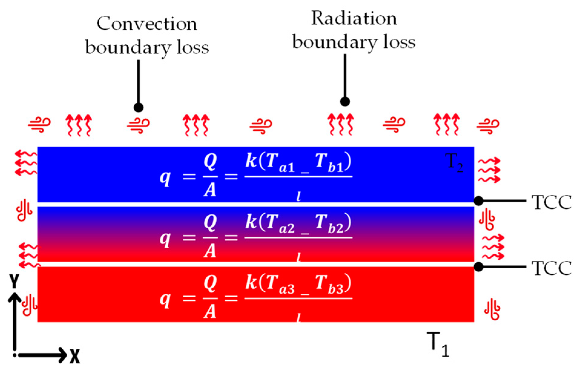
3.1. Heat Transfer Governing Equations

The transient governing equation for one-dimensional heat transfer and the considered boundary conditions for numerical TCC modelling are shown in Equations (6)–(8):
V f ρ c P T t = k e 2 T x 2 + Q ˙ h T T σ ε ( T 4 T 4 )
At the bottom surface at x = 0, the Dirichlet temperature boundary condition is defined to match the experimentally measured temperature T1 as follows:
T 0 , t = T 1 ( t )
On the top surface at x = H, heat losses due to convection and radiation are defined as follows based on the experimental data. The internal heat generation term is omitted in this scenario:
k e T x x = H = h [ T H , t T , t ] + σ [ T 4 H , t T 4 , t ]  
To model anisotropic heat transfer in production-scale preforms, conduction was identified as the dominant mode, with additional energy losses due to radiation and natural convection. These losses arose from heat sinks outside heating zones, air convection driven by temperature gradients, and radiative emission. The conservation of energy principle was applied to formulate the governing equations for both transient and steady-state conditions shown in Equations (9) and (10). Q ˙ is the internal heat generation term and the operator denotes the gradient operator.
v f ( ρ c P ) T t = k T + Q ˙ h T T σ ε ( T 4 T 4 )
k T + Q ˙ h T T σ ε T 4 T 4 = 0
In the above equations, Vf represents the volume fraction of the carbon fabric, while ρ denotes the effective density. The specific heat capacity is indicated by cP, and T is the temperature of the material at time t. The effective thermal conductivity is represented by ke, with x serving as the spatial coordinate and H indicating the thickness of the carbon fabric. The term T1 refers to the experimentally measured temperature at the bottom surface, whereas T(H, t) is the temperature at the top surface. Additionally, T signifies the ambient air temperature, h is the convection heat transfer coefficient, ϵ indicates emissivity, and σ represents the Stefan–Boltzmann constant [78,79]. Since woven fabrics are highly anisotropic materials, the heat conduction can be modelled using the anisotropic thermal conductivity, the corresponding thermal gradient and respective heat flux as shown in Equation (11):
k i j 2 T x i x j + Q ˙ = ρ c p T t Q c o n v e t i o n Q r a d i a t i o n
For the fully anisotropic model, all the elements in the conductivity matrix are to be determined. To simplify the model, the material model is assumed to be orthotropic with conductivities considered in three principal directions and k11 is equal to k22 due to the structured woven nature of the preform. The k33 term represents the through-thickness direction thermal conductivity as shown in Equation (12), which is the resultant effective conductivity (ke) computed using Equation (5).
q 1 q 2 q 3 = k 11 0 0 0 k 22 0 0 0 k 33 × Δ T 1 Δ T 2 Δ T 3
where k i j is the conductivity in the respective “ij” location in matrix form to completely represent the anisotropic thermal material properties.

3.2. TCC Parameter Tuning in Multilayer Coupon Stacks

To replicate the experimental heating process for the coupon models, a ply-wise finite element (FE) model was developed in Abaqus to simulate one-dimensional (1D) transient heat transfer through the thickness of compacted plies as shown in Figure 6. Each carbon fabric ply was represented as a homogenised layer composed of woven fabric with a 3.4 wt% binder at the interface, with material properties derived from prior experimental testing specific to this preform composition [34]. To account for the porous nature of the carbon fabric, a porosity-dependent volume fraction was applied to each ply, influencing heat transfer behaviour.
In this modelling framework, ply thickness was determined using a normalisation method (see Section 2.2), allowing for the introduction of a TCC parameter at each ply interface. The TCC parameter was applied to capture variations in contact effects between plies, enabling a more accurate representation of the thermal response across the preform structure. As illustrated in Figure 6, the model’s bottom boundary condition (BC) was based on experimentally measured temperature data, T1, while the top boundary conditions accounted for both natural convection and radiative losses. To incorporate ambient air temperature fluctuations due to heat loss, air temperature measurements were taken at three separate locations and integrated into the simulation. The numerical model parameters for TCC tuning are provided in Table 4, the parameter that needs to be tuned for each ply configuration is represented as xi and the temperature is compared with the experimental temperature.
The effects of phase change and the resultant thickness variation of the binder were not included in the model, as both specific heat and thermal conductivity parameters inherently account for the 3.6 wt% binder in the preform [34]. The TCC estimation can be performed using an analytical approach with experimental heat flux data or numerical heat flux data combined with temperature data in both cases. This is carried out to establish an empirical relationship between the number of layers and the TCC parameter in each configuration. With a defined convection heat transfer coefficient and emissivity for the top surface, the TCC was estimated by iteratively minimising the difference between simulated and experimentally measured top surface temperatures, T2. Additionally, multiple heating cycles demonstrated no significant impact on temperature evolution, further justifying the exclusion of these factors in the analysis. This approach simplifies the model while ensuring an accurate representation of the thermal behaviour within the preform. Positioning sensors between the top carbon fabric surface and the semi-transparent vacuum bag posed challenges in accurately determining the convection coefficient and emissivity of the top surface. To approximate the convection coefficient, the top surface temperature and ambient air temperature were initially used, based on empirical relations provided in Appendix B. Since the vacuum bag has a micrometre-scale thickness and is semi-transparent, it was omitted from the model, and adjusted convection and emissivity coefficients were instead applied directly to the top carbon fabric surface.
To further assess the uniqueness of parameter selection, additional simulations were conducted for each configuration of the coupon models exploring the variations across the parameter space. The mean simulation temperature for each configuration was analysed by varying the TCC, convection and emissivity within their respective parameter ranges. Specifically, TCC was varied by factors of 0.5, 1, 1.5, 2 and 2.5 relative to the initially tuned value. Convection coefficients were varied from 2 to 8 in increments of 2, while emissivity was adjusted from 0.2 to 0.8 in increments of 0.2. The results are compared with those obtained using the tuned parameters and the experimental data. An additional sensitivity analysis was performed by assuming the specific heat of the material to be temperature-independent. This simplification was applied across all configurations to assess the impact of this assumption on the temperature prediction in both the transient and steady-state regions.

3.3. Homogenised Production-Scale Preform Models

Figure 7a illustrates a half-section of the 30-ply preform configuration, including the associated components. The representative numerical model was developed in commercially available ABAQUS/standard 2023 software using a symmetric configuration along the primary axis to improve computational efficiency (See Figure 7b). The setup included 30- and 60-ply preforms with tooling, bagging and heater elements to replicate the preforming process that was geometrically modelled and meshed using DC3D8 8-node brick elements as shown in Figure 7b.
Thermal properties specific to the materials and their interactions, including conduction, convection and radiation, were defined as input parameters to closely replicate the experimental conditions, as outlined in Table 5. Contact conductance at the material interfaces was determined by correlating the temperature differences across the interfaces with heat flux values recorded by sensors positioned above the silicone membrane. The calculated contact conductance values were 6700 W/m2 °C for the heater-to-tool interface, 1247 W/m2 °C for the silicone-to-CF interface, 23.69 W/m2 °C between silicone membranes, and 68 W/m2 °C for the tool-to-silicone interface. These contact interactions are defined as surface-to-surface contact with master and slave nodes based on the mesh size of individual instances. A grid dependency analysis was performed to refine the mesh of linear hexahedron elements, ensuring a balance between computational accuracy and efficiency. To capture the temperature gradient in the thickness direction of the preforms and other materials in the model, edge seeding was utilised. Volumetric heat flux values, derived from the energy consumption data of individual heater elements during the DDPF cycle experiment, were applied as boundary conditions to the heater element geometry (see Figure 7b) to simulate the heating process. Finally, the simulation temperature is compared in three distinct locations in the thickness direction of each zone with experimental data. These locations include the bottom, middle and top of the preform as they are the primary locations to ensure the preform temperature for a set heater temperature.

4. Results and Discussion

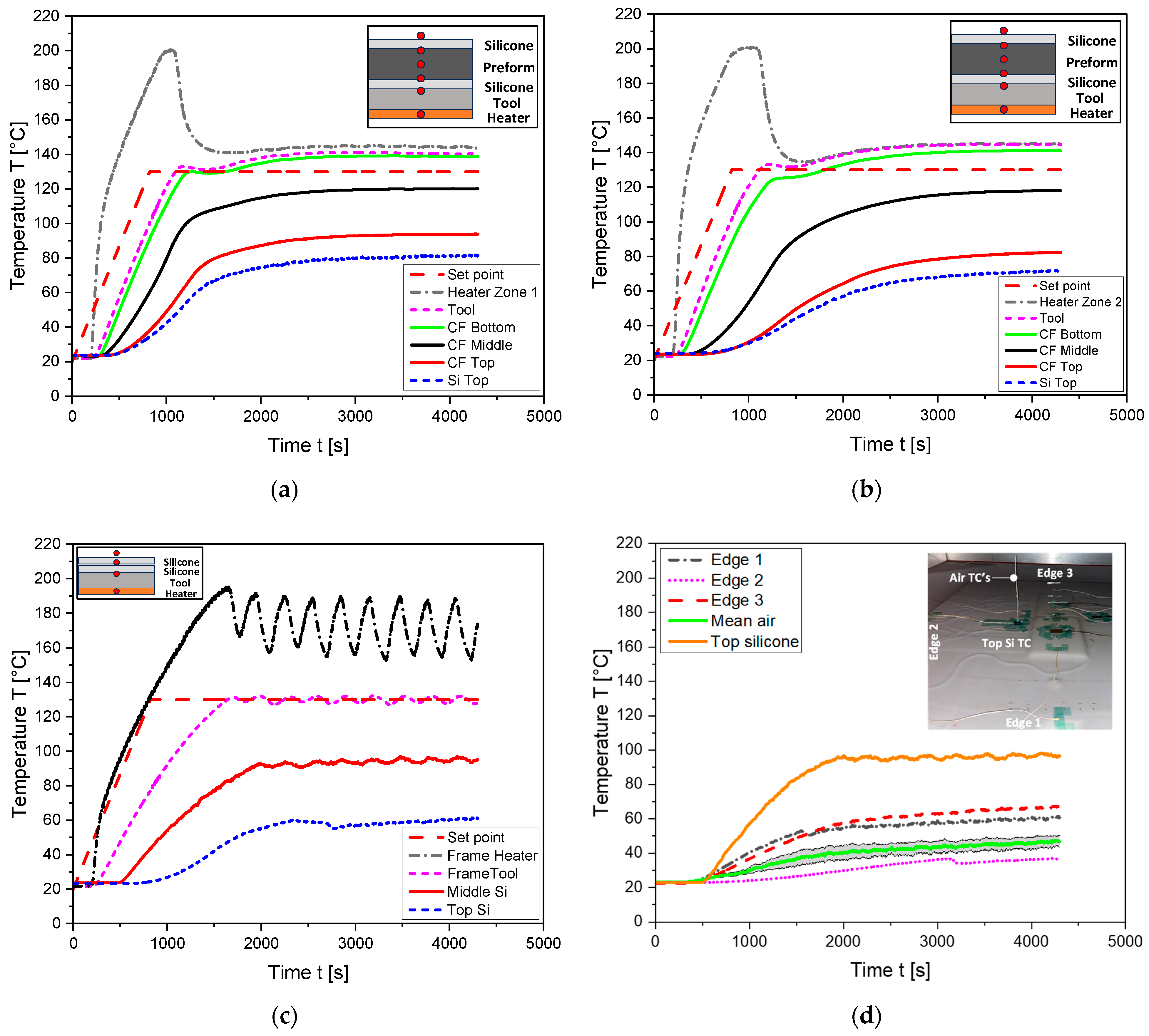
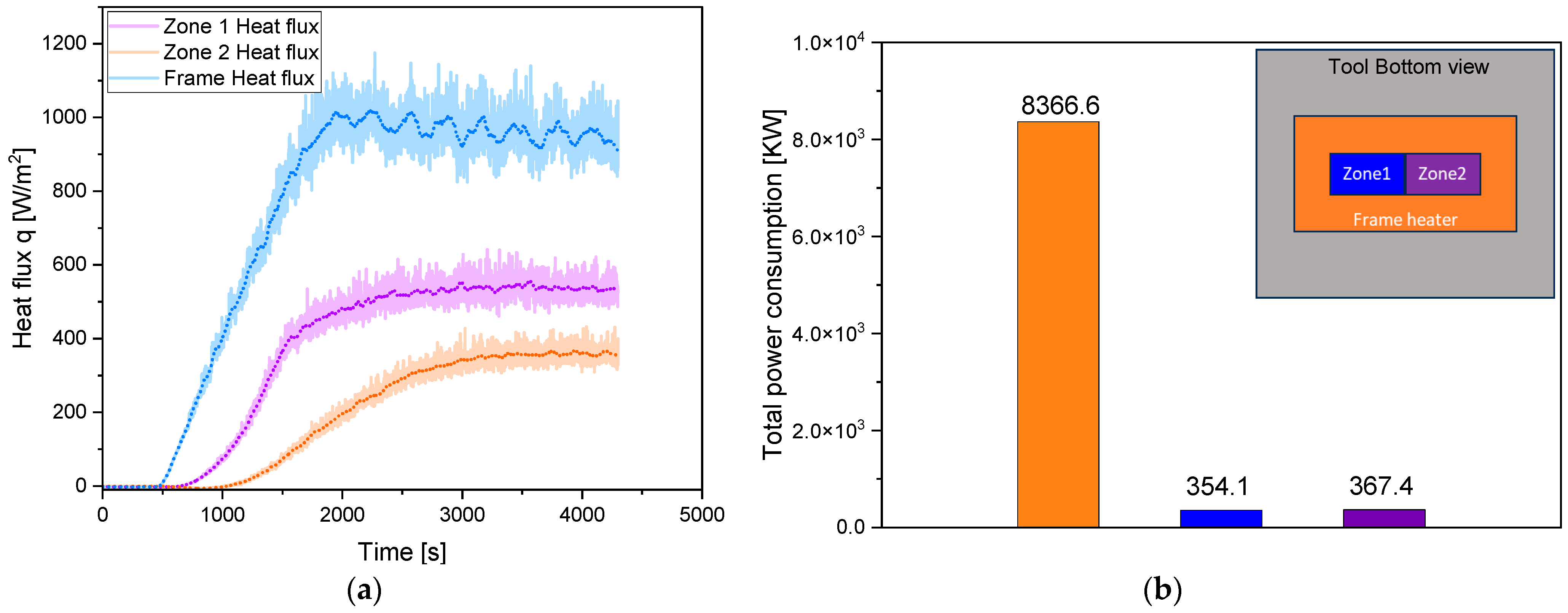
4.1. DDPF Process Experimental Results

Figure 8a–d show the temperature evolution at various locations within the experimental setup, including the heater elements, carbon preforms, tool surface, the top layer of silicone rubber, and the surrounding air, as a function of time in zone 1 (Figure 8a), zone 2 (Figure 8b) and the outside active zone. The heater output is controlled by the tool’s TC, positioned on the surface directly above the heater element. The set-point temperature, aimed at activating the carbon preform, is set to 130 °C, ensuring that a temperature of 120 °C is achieved beneath the preform. At this set point, the heater elements reach a peak temperature of approximately 200 °C during the ramp-up phase.
Heaters one and two stabilise after about 1300 s, while the frame heater exhibits oscillatory behaviour, fluctuating between 160 °C and 200 °C, as shown in Figure 8c to counter the heat losses from tooling. This fluctuation compensates for heat losses from the tooling, with oscillations arising from the periodic energy supply from the frame heater to the tool. This ensures the preform maintains its set-point temperature, regulated by the third control thermocouple, which is connected to the controller and positioned above the tool outside the active heating zone.
Figure 8d shows the evaluation of experimental temperature at edge locations of the tool and the ambient air temperature close to the active preform zone. Zone 2, which contains 60 plies, exhibits a slower temperature increase during the ramp-up phase and a lower stabilised top temperature compared to zone 1. This behaviour is attributed to the increased thermal mass due to the additional 30 plies. Furthermore, the top surface temperature of the silicone bagging is higher in the tool’s active zones compared to the edge regions, reflecting localised heat concentration near the heater elements. For the bottom heating configuration, the mean ambient air temperature above the silicone surface was measured at distances of 20 mm, 120 mm, and 220 mm. As shown in Figure 8d, the air temperature reaches a maximum mean value of 45 °C due to convective heat transfer losses, implicating some of the inherent losses in the process.
In addition to the temperature data, Figure 9a,b present the heat flux leaving the top surface and energy consumption of the heater elements over a cycle duration of 4500 s.
Heat flux analysis reveals a linear heat transfer rate in the frame heater region during the ramp-up phase, in contrast to the nonlinear behaviour observed in the 30- and 60-ply preform regions. In the quasi-steady-state region, the stabilised heat transfer rates are 954 W/m2, 537 W/m2 and 356 W/m2 for the frame heater, 60-ply region and 30-ply region, respectively. The presence of additional carbon fabrics in zone 2 reduces the through-thickness heat transfer rate, potentially leading to longer cycle times. Energy consumption, derived from voltage and current data recorded by the controller, shows higher energy use in the frame heater compared to heaters one and two located in the active zones. Initially, all three heaters contribute to raising the material temperature. However, during the holding phase, only the frame heater remains active to maintain the desired temperature. Total energy consumption for the frame heater is 8366.6 kW, while heaters one and two consume 354.1 kW and 367.4 kW, respectively.

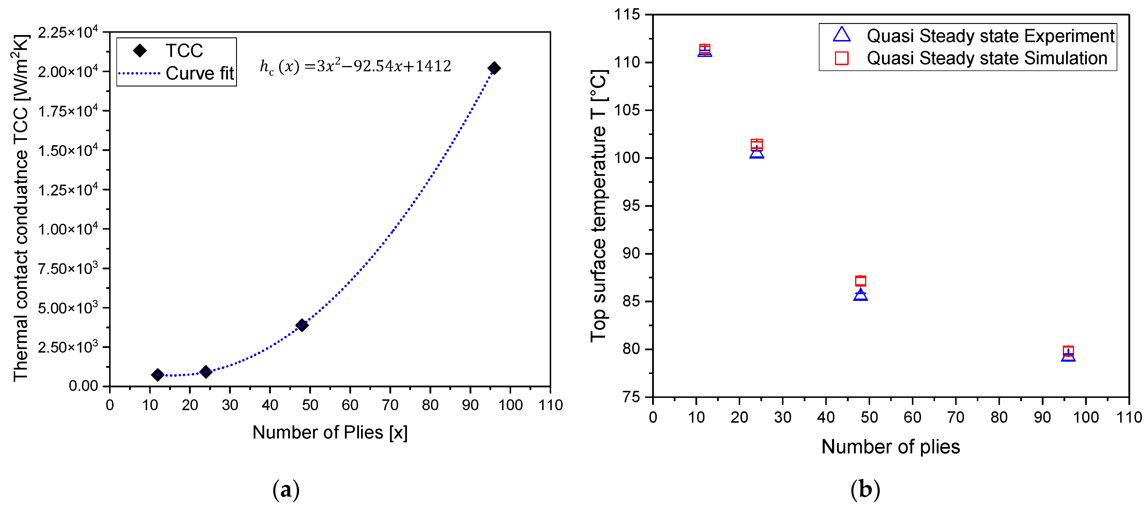
4.2. TCC Parameter Coupon Numerical Tuning and Experimental Validation Study

This study aims to develop an empirical TCC relationship for multilayer coupon stacks by using a combined numerical and experimental approach. Three cases of 12, 24 and 48 are utilised to develop the TCC relation, and 96 layers are utilised for validation of the developed empirical relation. The experimental evaluation initially demonstrated that with an increase in the number of layers, heat transfer in the thickness direction reduces. The numerically tuned TCC parameters for different ply counts are presented in Figure 10a, and the quasi-steady state temperature comparison of numerical and experimental top surface temperatures is shown in Figure 10b, with good agreement.
During the ramp-up phase, the ramp rates for 12, 24 and 48 layers are 20.12 °C/min, 14.53 °C/min and 8.86 °C/min, respectively, with a quasi-steady temperature difference of 9 °C, 18.5 °C and 32.2 °C, respectively. In the case of 96 layers, the ramp rate was initially 4.18 °C/min, before the temperature evaluation rose nonlinearly and finally attained a temperature difference of 40 °C in the quasi-steady-state region. For the numerically tuned TCC values of 734 W/m2 °C, 921 W/m2 °C and 3890 W/m2 °C for 12-, 24- and 48-ply stacks, the simulated temperature predications are in good agreement with the experimental results. By using these three points of data, curve fitting was carried out to obtain a TCC value for 96-ply stacks, which resulted in a TCC value of 20,208 W/m2 °C, which predicts the top surface temperature accurately. The curve-fitted empirical relationship between the TCC parameter and the number of plies is shown in Equation (13), with an R-squared value of 0.999. When this equation is used in conjunction with Equation 8, the effective through-thickness bulk conductivity of the stack can be estimated for numerical preforming heat transfer simulations.
h c x = 3 x 2 92.54 x + 1412
In addition to this steady state, the transient effects of the tuned TCC parameter are also analysed on the numerically predicted top surface temperature for 12, 24, 48 and 96 layers as shown in Figure 11a–d. These results for multilayer coupon stacks reveal specific trends related to heat transfer mechanisms and the influence of external convection factors in the transient domain. For thinner stacks, such as the 12- and 24-layer configurations as shown in Figure 11a,b, the experimental and simulation results align closely, as heat conduction dominates, and external factors have minimal impact. Heat energy dissipates efficiently through the material, resulting in consistent temperature profiles. In thicker stacks, particularly the 96-layer configuration as shown in Figure 11d, the experimental results deviate from the simulations due to slower heat conduction through the stack thickness.
Additionally, the vacuum bag, a micrometre-thick layer covering the stack and heater tool outside the preform perimeter, heats rapidly and influences heat transfer at the top surface TC sensor. Surrounding air above the vacuum bag also heats up and circulates, especially during the initial stages of the heating cycle. This external convective heat transfer affects the temperature readings at the top thermocouple sensor, particularly in the 96-layer stack, where heat dissipation through the material is slower. The effect is less pronounced in the 48-layer stack as shown in Figure 11c but still contributes to minor deviations. Despite these limitations, all configurations reliably predict the quasi-steady-state top temperatures of the preforms for a given bottom temperature, highlighting the model’s effectiveness in capturing thermal equilibrium.
The parametric sensitivity analysis for configurations 12, 24, 48 and 96 shows that variations in TCC have a minor effect on the transient response, while the overall mean temperature remains within the experimental standard deviation except for 96. The standard deviation visualisation highlights sensitivity, particularly during heating, suggesting that multiple parameter sets can yield similar results. This confirms the presence of multiple local minima in the parameter space, influencing sensitivity but not significantly altering the final temperature trend. This behaviour is driven by the interdependence of TCC, convection, and emissivity, where changes in one parameter can offset another. Additionally, the temperature-dependent nature of TCC and convection, along with model simplifications, contribute to multiple valid solutions within the bounds of experimental uncertainty. The temperature sensitivity study showed a slight increase in predicted temperatures, both in the transient and steady-state regions, with variations under +2 °C across all configurations. As the number of layers increased, the temperature prediction slightly rose, indicating that assuming a temperature-independent specific heat results in slightly higher temperature predictions, especially in the configuration with high ply counts.

4.3. Homogenised Production-Scale Preform Model Validation

The numerical model developed in ABAQUS was validated against experimental temperature data for both 30-ply and 60-ply dry fabric preforms, demonstrating strong agreement across multiple measurement locations, as shown in Figure 12. The model accurately predicted the temperature behaviour during the quasi-steady state, but some discrepancies were observed during the ramp-up, particularly at the top surface. For the 30-ply preform, the predicted peak temperature at the bottom surface reached approximately 133 °C, with a deviation of 4 °C (2.92%). At the mid-plane, deviations of 7 °C (5.93%) were observed, while the top surface temperature during steady-state conditions showed a deviation of 2 °C (2.17%), as shown in Figure 12a. For the 60-ply preform, the peak temperature at the bottom surface was predicted to be around 133 °C, with a deviation of 3 °C (2.21%). The mid-plane exhibited a deviation of 6 °C (5.17%), and the top surface showed a deviation of 2 °C (2.38%) during steady-state conditions. During the ramp-up phase, the model’s accuracy varied in predicting the ramp rates, as shown in Figure 12b.
For the 30-ply preform, the experimental ramp rates were 0.12 °C/s at the bottom, 0.09 °C/s in the middle, and 0.059 °C/s at the top. The simulation predicted ramp rates of 0.11 °C/s at the bottom, 0.08 °C/s in the middle, and 0.061 °C/s at the top. This numerical correlation indicates that the model slightly underpredicted the ramp rates at the bottom and middle, with deviations of 3% and 8%, respectively, while closely matching the top ramp rate with a deviation of 3.3%. For the 60-ply preform, the experimental ramp rates were 0.119 °C/s at the bottom, 0.072 °C/s in the middle, and 0.035 °C/s at the top. The simulation predicted ramp rates of 0.115 °C/s at the bottom, 0.07 °C/s in the middle, and 0.044 °C/s at the top. The model slightly underpredicted the ramp rates at the bottom and middle, with deviations of 3.7% and 3%, respectively, while overpredicting the ramp rate at the top with a deviation of 20%. These observed discrepancies, particularly during the ramp-up phase, can largely be attributed to the limitations of the numerical model in accounting for certain factors inherent in the experimental setup such as the convection losses, radiation exchange with the top IR heater array and assumed in-plane conductivity for fabrics.
The numerical nodal temperature distribution at the end of 4100 s is presented in Figure 13a,b, showing temperature gradients in the model indicating the inherent heat losses in the tool setup and preforms. To optimise this and minimise the heat losses, efficiency studies are necessary, with changes in the experimental strategy to minimise convection and radiation heat losses.
One key factor is the silicone membrane heating up faster outside the preform active zone in the experimental setup, which is located directly on the frame heater. This rapid heating of the silicone membrane creates localised airflow. It affects the sensor measurements at the top location, causing it to reach higher temperatures before the top location of the preform. Additionally, the high emissivity of the IR heater elements likely increases radiative heat absorption, altering the localised thermal environment and influencing the airflow patterns and radiative heat transfer, especially at the top surface.
These interactions, simplified in the model, may explain the overprediction of temperature, particularly at the top surface during the ramp-up phase. In terms of modelling, for this internal heat generation model, time step integration also had an effect on the predicted temperature, with lower time integrations leading to accurate temperature predictions. Based on these validation results, it is evident that the model should include additional heat loss factors at the top location and incorporate accurate in-plane conductivity of the fabrics. Currently, the model assumes the in-plane conductivity to be ten times that of the through-thickness direction [80]. These refinements would help reduce the observed deviations and significantly enhance the model’s accuracy in capturing the transient behaviour, providing more precise temperature predictions across different preform thicknesses.

5. Conclusions

A numerical model was developed to simulate the heat transfer dynamics of the DDPF process, with a particular emphasis on multilayer preform configurations. This model integrates experimentally derived TCC data to predict temperature distributions and assess energy efficiency across different stack thicknesses and material properties. Key parameters considered in the simulation include localised temperature gradients, thermal contact resistance and material thermal conductivity.
The model showed strong agreement with experimental data, accurately capturing both steady-state and transient thermal behaviours. Results revealed that maintaining uniform temperature profiles becomes progressively more challenging as stack thickness increases, primarily due to variations in thermal contact resistance. While discrepancies were observed during the ramp-up phase due to external convection effects, the overall predictive accuracy and reliability of the model were validated.
Future work should focus on integrating multi-physics phenomena, including air convection, preform thickness changes, and radiative heat transfer, to enhance modelling accuracy. Additionally, efforts should aim to develop adaptive heating systems, optimise energy-efficient processes, and conduct a comprehensive full-scale computational fluid dynamics (CFD) study to improve the reliability and efficiency of multilayer preforming.

Author Contributions

S.D.: writing—original draft, methodology, software, investigation, formal analysis, data curation, conceptualisation, visualisation, validation. S.G.: writing—original draft, formal analysis, data curation. M.R.: writing—review and editing, formal analysis, supervision, methodology, conceptualisation, project management. J.N.: writing—review and editing, supervision. A.D.P.: writing—review and editing, funding acquisition. All authors have read and agreed to the published version of the manuscript.

Funding

This research was funded by the Victorian Higher Education State Investment Fund (VHESIF) through the Aerostructures Innovation Research Hub (AIR Hub).

Data Availability Statement

Data will be made available on request from the corresponding author due to legal reasons.

Acknowledgments

The authors acknowledge the support of the Victorian Government through the Victorian Higher Education State Investment Fund (VHESIF), as well as the Swinburne/CSIRO Industry 4.0 Test Lab. Special thanks are extended to the digitalisation team of the AIR Hub at Swinburne University of Technology for their invaluable assistance throughout this project. The authors gratefully acknowledge Victoria Zinnecker for her critical insights and continued support, which were vital to the success of this study. The authors also thank Muzaffar Chumroo for his help in setting up the MTS experimental apparatus. Finally, the authors extend their gratitude to Boeing Research & Technology—Australia for their support and collaboration, which played a crucial role in the successful completion of this industry-focused project.

Conflicts of Interest

The authors declare that they have no known competing financial interests or personal relationships that could have appeared to influence the work reported in this paper.

Appendix A

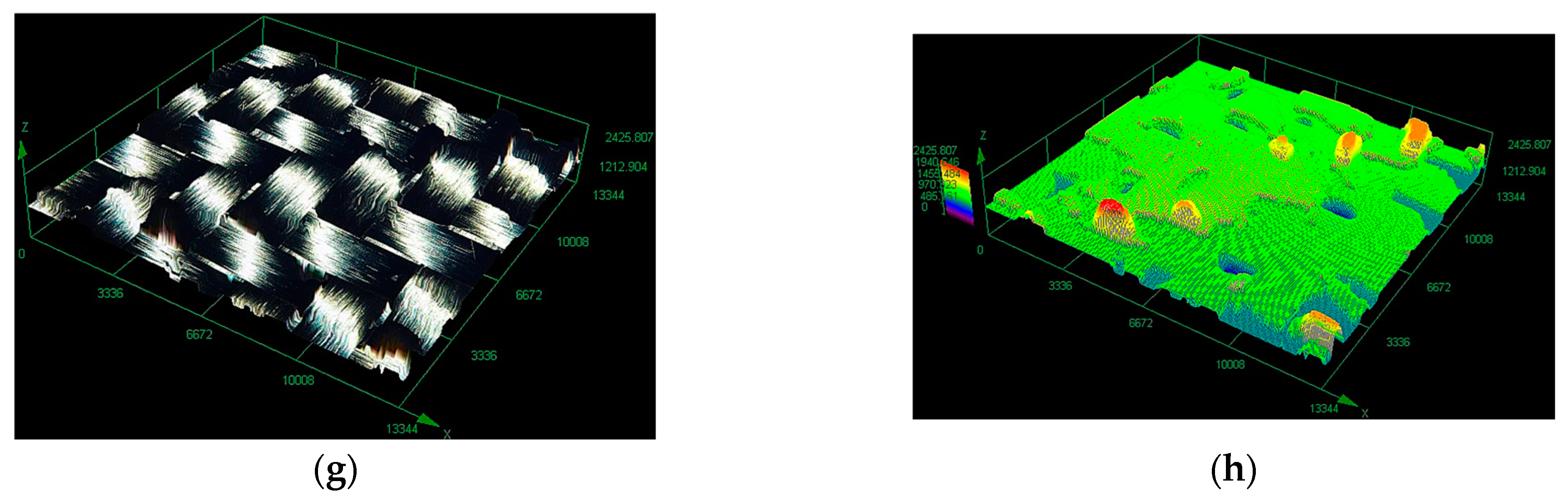
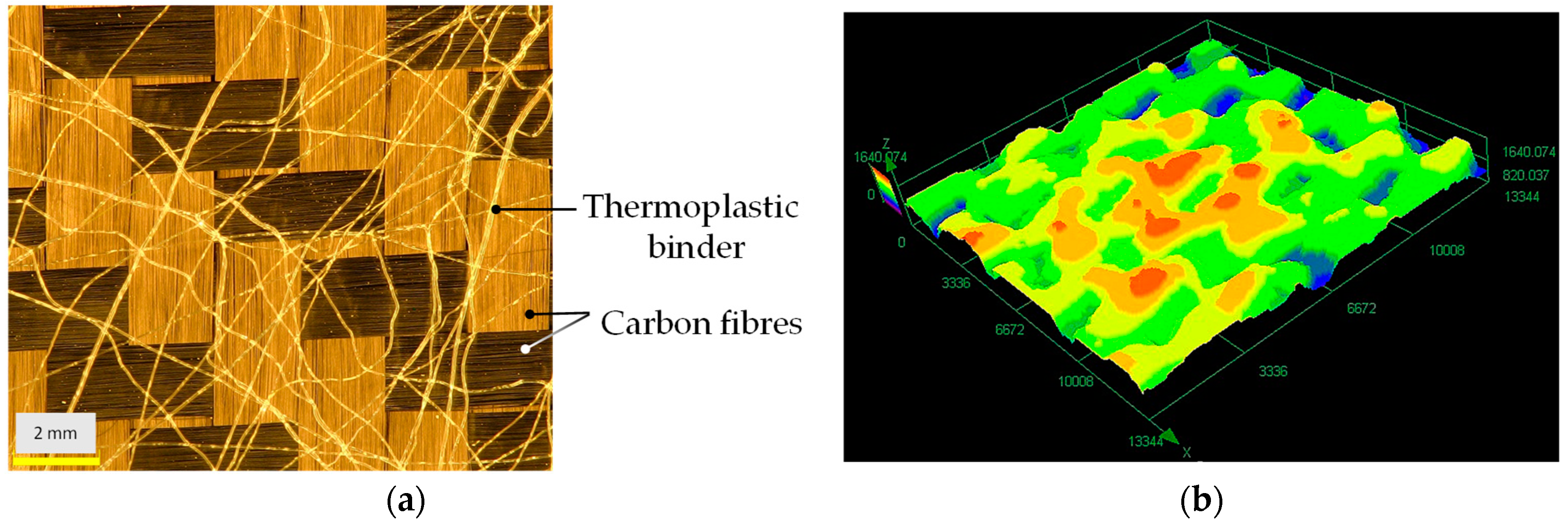
  • Optical images and micrographs of coupon model surface asperities following de-compaction at the tool–material interface.
The surface morphology investigations provide deeper insights into morphological changes, including variations in surface roughness, asperity deformation and material redistribution. These factors are critical in understanding how the number of carbon fabric layers subjected to the same compression load results variations in thickness and volume fraction at both yarn and preform levels in each preform configuration. Such variations influence interfacial contact, altering the contact area and pressure distribution which directly impact the heat transfer. This supports the assumption of a variable TCC parameter at the interfaces of each preform configuration.
Figure A1. Optical images and micrographs of coupon model surface asperities following decompaction at the tool–material interface—12 layers—(a,b); 24 layers—(c,d); 48 layers—(e,f); 96 layers—(g,h).
Energies 18 01471 g0a1aEnergies 18 01471 g0a1b

Appendix B

  • Estimation of convection coefficient in natural heating.
To calculate the convection coefficient in the experimental closed DDPF setup, heat transfer begins as the heating process warms the stack and bagging from the bottom. The heated air above the bagging becomes less dense and rises, creating unstable natural convection. The convection coefficient is estimated using surface and air temperatures, governed by fluid dynamics relationships involving the Nusselt, Rayleigh, Grashof, and Prandtl numbers. The convection coefficient is related to the Nusselt number (Nu) through Equation (A1):
N u = h L k
where h is the convection coefficient, k is the thermal conductivity of air and L is the characteristic length of the surface. For natural convection, the Nusselt number depends on the Rayleigh number (Ra) as shown in Equations (A2) and (A3).
N u = 0.54 R a 1 4                         f o r   ( 10 4 < R a < 10 7 )
N u = 0.54 R a 1 3                         f o r   ( 10 7 < R a < 10 11 )
The Rayleigh number is expressed as product of the Grashof (Gr), and Prandtl (Pr) numbers, which quantify buoyancy forces to viscous forces and the ratio of momentum diffusivity to thermal diffusivity, respectively, as shown in Equations (A5) and (A6):
R a = G r × P r
G r = g β T L 3 ν 2
P r = ν α
Here, g is gravitational acceleration, β is the thermal expansion coefficient, ΔT is the temperature difference, ν is the kinematic viscosity and α is the thermal diffusivity. In addition, the convection coefficient is also influenced by the surface shape and scale, with the characteristic length varying based on the surface area-to-perimeter ratio for 1D, 2D, or 3D configurations, as shown in Figure A2. The location of the heating surface (top or bottom) further impacts the convection coefficient by stabilising or destabilising airflow, thereby affecting the convective heat transfer behaviour.
Figure A2. Variation in the convection coefficient with surface temperature for (a) the convection coefficient h in a 1D geometry with a characteristic length of 0.1 mm and (b) the effective convection coefficient h* in a 3D geometry with a characteristic length of 0.025 mm.
Energies 18 01471 g0a2

References

  1. Lawrence, G.D.; Chen, S.; Warrior, N.A.; Harper, L.T. Preforming of Multi-Ply Non-Crimp Fabric Laminates Using Double Diaphragm Forming. In Proceedings of the Twenty-Third International Conference on Composite Materials, ICCM 23, Belfast, UK, 1 August 2023. [Google Scholar]
  2. Pantelakis, S.G.; Baxevani, E.A. Optimization of the Diaphragm Forming Process with Regard to Product Quality and Cost. Compos. Part Appl. Sci. Manuf. 2002, 33, 459–470. [Google Scholar] [CrossRef]
  3. Chen, S.; McGregor, O.P.L.; Harper, L.T.; Endruweit, A.; Warrior, N.A. Optimisation of Local In-Plane Constraining Forces in Double Diaphragm Forming. Compos. Struct. 2018, 201, 570–581. [Google Scholar] [CrossRef]
  4. Channer, K.J.; Cosgriff, W.; Smith, G.F.; Okoli, O.I. Development of the Double RIFT Diaphragm Forming Process. J. Reinf. Plast. Compos. 2002, 21, 1629–1635. [Google Scholar] [CrossRef]
  5. Solvay Unveils Double Diaphragm Forming (DDF) Automated Demonstrator Line. Available online: https://www.solvay.com/en/press-release/solvay-unveils-ddf-line (accessed on 20 June 2024).
  6. Hot Drape Forming—Preforming Solutions. Available online: https://old.pinetteemidecau.eu/en/equipment-and-systems/forming/preforming-solutions (accessed on 20 June 2024).
  7. Kunz, H.; Löchte, C.; Dietrich, F.; Raatz, A.; Fischer, F.; Dröder, K.; Dilger, K. Novel Form-Flexible Handling and Joining Tool for Automated Preforming. Sci. Eng. Compos. Mater. 2015, 22, 199–213. [Google Scholar] [CrossRef]
  8. Bian, X.X.; Gu, Y.Z.; Sun, J.; Li, M.; Liu, W.P.; Zhang, Z.G. Effects of Processing Parameters on the Forming Quality of C-Shaped Thermosetting Composite Laminates in Hot Diaphragm Forming Process. Appl. Compos. Mater. 2013, 20, 927–945. [Google Scholar] [CrossRef]
  9. Yu, F.; Chen, X.; Chen, S.; Harper, L.T. Numerical Study on the Formation of Defects During Double Diaphragm Forming Using a Biaxial Non-Crimp Fabric. In Proceedings of the 10th Chinese Society of Aeronautics and Astronautics Youth Forum; Chinese Society of Aeronautics and Astronautics, Ed.; Springer Nature: Singapore, 2023; pp. 392–402. [Google Scholar]
  10. Ning, H.; Vaidya, U.; Janowski, G.M.; Husman, G. Design, Manufacture and Analysis of a Thermoplastic Composite Frame Structure for Mass Transit. Compos. Struct. 2007, 80, 105–116. [Google Scholar] [CrossRef]
  11. Chen, S.; McGregor, O.P.L.; Endruweit, A.; Elsmore, M.T.; De Focatiis, D.S.A.; Harper, L.T.; Warrior, N.A. Double Diaphragm Forming Simulation for Complex Composite Structures. Compos. Part Appl. Sci. Manuf. 2017, 95, 346–358. [Google Scholar] [CrossRef]
  12. Thompson, A.J.; McFarlane, J.R.; Belnoue, J.P.-H.; Hallett, S.R. Numerical Modelling of Compaction Induced Defects in Thick 2D Textile Composites. Mater. Des. 2020, 196, 109088. [Google Scholar] [CrossRef]
  13. Thompson, A.J.; Belnoue, J.P.-H.; Hallett, S.R. Modelling Defect Formation in Textiles during the Double Diaphragm Forming Process. Compos. Part B Eng. 2020, 202, 108357. [Google Scholar] [CrossRef]
  14. Wambua, P.M.; Anandjiwala, R. A Review of Preforms for the Composites Industry. J. Ind. Text. 2011, 40, 310–333. [Google Scholar] [CrossRef]
  15. Krebs, J.; Bhattacharyya, D.; Friedrich, K. Production and Evaluation of Secondary Composite Aircraft Components—A Comprehensive Case Study. Compos. Part Appl. Sci. Manuf. 1997, 28, 481–489. [Google Scholar] [CrossRef]
  16. Krebs, J.; Friedrich, K.; Bhattacharyya, D. A Direct Comparison of Matched-Die versus Diaphragm Forming. Compos. Part Appl. Sci. Manuf. 1998, 29, 183–188. [Google Scholar] [CrossRef]
  17. Yu, X.; Zhang, L.; Mai, Y.W. Modelling and Finite Element Treatment of Intra-Ply Shearing of Woven Fabric. J. Mater. Process. Technol. 2003, 138, 47–52. [Google Scholar] [CrossRef]
  18. Wang, L.; Wang, J.; Liu, M.; Peng, X. Development and Verification of a Finite Element Model for Double Diaphragm Preforming of Unidirectional Carbon Fiber Prepreg. Compos. Part Appl. Sci. Manuf. 2020, 135, 105924. [Google Scholar] [CrossRef]
  19. Kondratiev, A.; Purhina, S.; Shevtsova, M.; Tsaritsynskyi, A. Thermodynamic Model of Self-Heating Mold for the Energy Efficient Composite Manufacturing. In Proceedings of the 2021 IEEE 2nd KhPI Week on Advanced Technology, Kharkiv, Ukraine, 13–17 September 2021; pp. 120–125. [Google Scholar] [CrossRef]
  20. Widmaier, N.; Radjef, R.; Middendorf, P.; Fox, B. Double Diaphragm Forming of Bindered Unidirectional Dry-Fibre Tapes: Experimental Analysis of Forming Temperature. In Proceedings of the 20th Australian International Aerospace Congress, Melbourn, Australia, 27 February 2023; Engineers Australia: Melbourne, Australia, 2023. [Google Scholar]
  21. Miris, G.; Ravandi, M.; Cardew-Hall, A.; Eisenbart, B.; Di Pietro, A. Efficient Numerical Analysis of In-Plane Compression-Induced Defects in Thick Multi-Ply Woven Textile Preforms during Double Diaphragm Forming. Compos. Part Appl. Sci. Manuf. 2024, 186, 108431. [Google Scholar] [CrossRef]
  22. Matsudaira, M.; Qin, H. Features and Mechanical Parameters of a Fabric’s Compressional Property. J. Text. Inst. 1995, 86, 476–486. [Google Scholar] [CrossRef]
  23. Chen, B.; Chou, T.-W. Compaction of Woven-Fabric Preforms in Liquid Composite Molding Processes: Single-Layer Deformation. Compos. Sci. Technol. 1999, 59, 1519–1526. [Google Scholar] [CrossRef]
  24. Chen, B.; Chou, T.W. Compaction of Woven-Fabric Preforms: Nesting and Multi-Layer Deformation. Compos. Sci. Technol. 2000, 60, 2223–2231. [Google Scholar] [CrossRef]
  25. El-Dessouky, H.M.; Lawrence, C.A. Ultra-Lightweight Carbon Fibre/Thermoplastic Composite Material Using Spread Tow Technology. Compos. Part B Eng. 2013, 50, 91–97. [Google Scholar] [CrossRef]
  26. Ohlsson, F. An Introduction to Spread Tow Reinforcements. Part 2: Design and Applications. Reinf. Plast. 2015, 59, 228–232. [Google Scholar] [CrossRef]
  27. Zheng, Z.; Wang, H.; Zhao, X.; Zhang, N. Simulation of the Effects of Structural Parameters of Glass Fiber Fabric on the Thermal Insulation Property. Text. Res. J. 2018, 88, 1954–1964. [Google Scholar] [CrossRef]
  28. Snape, A.E.; Turner, J.L.; El-Dessouky, H.M.; Saleh, M.N.; Tew, H.; Scaife, R.J. Stabilising and Trimming 3D Woven Fabrics for Composite Preforming Applications. Appl. Compos. Mater. 2018, 25, 735–746. [Google Scholar] [CrossRef]
  29. Wu, W.; Jiang, B.; Xie, L.; Klunker, F.; Aranda, S.; Ziegmann, G. Effect of Compaction and Preforming Parameters on the Compaction Behavior of Bindered Textile Preforms for Automated Composite Manufacturing. Appl. Compos. Mater. 2013, 20, 907–926. [Google Scholar] [CrossRef]
  30. Wei, K.; Liang, D.; Mei, M.; Wang, D.; Yang, X.; Qu, Z. Preforming Behaviors of Carbon Fiber Fabrics with Different Contents of Binder and under Various Process Parameters. Compos. Part B Eng. 2019, 166, 221–232. [Google Scholar] [CrossRef]
  31. Bulat, M.; Heieck, F. Binder Application Methods for Textile Preforming Processes. LTH Faserverbund-Leichtbau; FL 21 200-02; Luftfahrttechnisches Handbuch: Braunschweig, Germany, 2015; pp. 1–16. [Google Scholar]
  32. Tonejc, M.; Ebner, C.; Fauster, E.; Schledjewski, R. Influence of Test Fluids on the Permeability of Epoxy Powder Bindered Non-Crimp Fabrics. Adv. Manuf. Polym. Compos. Sci. 2019, 5, 128–139. [Google Scholar] [CrossRef]
  33. Terekhov, I.V.; Chistyakov, E.M. Binders Used for the Manufacturing of Composite Materials by Liquid Composite Molding. Polymers 2021, 14, 87. [Google Scholar] [CrossRef]
  34. Dandangi, S.; Ravandi, M.; Naser, J.; Di Pietro, A. Thermophysical Characterization of Materials for Energy-Efficient Double Diaphragm Preforming. Energies 2024, 17, 3758. [Google Scholar] [CrossRef]
  35. Estrada, G.; Line Vieux-Pernon, C.É.; Advani, S.G. Experimental Characterization of the Influence of Tackifier Material on Preform Permeability. J. Compos. Mater. 2002, 36, 2297–2310. [Google Scholar] [CrossRef]
  36. Nezami, F.N.; Gereke, T.; Cherif, C. Isothermal Multisection Tooling for the Automated Preforming of Carbon Fiber Composite Structures. Key Eng. Mater. 2014, 611–612, 349–355. [Google Scholar] [CrossRef]
  37. Weiland, J.S.; Hubert, P.; Hinterho lzl, R. Thermal Dimensioning of Manufacturing Moulds with Multiple Resistively Heated Zones for Composite Processing. J. Compos. Mater. 2017, 51, 3969–3986. [Google Scholar] [CrossRef]
  38. Aranda, S.; Klunker, F.; Ziegmann, G. Influence of the Binding System on the Compaction Behaviour of NCF Carbon Fibre Reinforcements. In Proceedings of the ICCM 18: International Conferences on Composite Materials, Jeju, Republic of Korea, 21–26 August 2011; ICCM: Jeju, Republic of Korea, 2011. [Google Scholar]
  39. Schnurr, R.; Gabriel, F.; Beuscher, J.; Dröder, K. Model-Based Heating and Handling Strategy for Pre-Assembled Hybrid Fibre-Reinforced Metal-Thermoplastic Preforms. In Proceedings of the 2nd CIRP Conference on Composite Material Parts Manufacturing, Sheffield, UK, 10 October 2019; Advanced Manufacturing Research Centre: Sheffield, UK, 2019. [Google Scholar]
  40. Zinnecker, V.; Cardew-Hall, A.; Reghat, M.; Ravandi, M.; Di, P.A. Mechanical Characterisation of Influencing Material Properties of Dry Carbon Fibre Reinforcement in a Double Diaphragm Forming Process. In Proceedings of the AIAC 2023: 20th Australian International Aerospace Congress, Melbourne, Australia, 16 June 2023; Engineers Australia: Melbourne, Australia, 2023; pp. 569–574. [Google Scholar]
  41. Miris, G.; Ravandi, M.; Zinnecker, V.; Eisenbart, B.; Di, P.A. Process Modelling of an Aero-Grade Hyperelastic Membrane for Double Diaphragm Forming Operations. In Proceedings of the AIAC 2023: 20th Australian International Aerospace Congress, Melbourne, Australia, 16 June 2023; Engineers Australia: Melbourne, Australia, 2023; pp. 563–568. [Google Scholar]
  42. Reghat, M.; Ravandi, M.; Zinnecker, V.; Di Pietro, A. Through-Thickness Thermal Conductivity Characterisation of Dry Carbon Fibre Fabric. Mater. Lett. 2024, 361, 136116. [Google Scholar] [CrossRef]
  43. Kearney, P.; Lekakou, C.; Belcher, S. Measurement of the Heat Transfer Properties of Carbon Fabrics via Infrared Thermal Mapping. J. Compos. Sci. 2022, 6, 155. [Google Scholar] [CrossRef]
  44. Zhou, T.; Zhao, Y.; Rao, Z. Fundamental and Estimation of Thermal Contact Resistance between Polymer Matrix Composites: A Review. Int. J. Heat Mass Transf. 2022, 189, 122701. [Google Scholar] [CrossRef]
  45. Zhao, D.; Qian, X.; Gu, X.; Jajja, S.A.; Yang, R. Measurement Techniques for Thermal Conductivity and Interfacial Thermal Conductance of Bulk and Thin Film Materials. J. Electron. Packag. 2016, 138, 040802. [Google Scholar] [CrossRef]
  46. Palacios, A.; Cong, L.; Navarro, M.E.; Ding, Y.; Barreneche, C. Thermal Conductivity Measurement Techniques for Characterizing Thermal Energy Storage Materials—A Review. Renew. Sustain. Energy Rev. 2019, 108, 32–52. [Google Scholar] [CrossRef]
  47. Mohammadi, M.; Banks-Lee, P.; Ghadimi, P. Determining Radiative Heat Transfer Through Heterogeneous Multilayer Nonwoven Materials. Text. Res. J. 2003, 73, 896–900. [Google Scholar] [CrossRef]
  48. Guo, J.; Chen, X.N.; Qu, Z.G.; Ren, Q.L. Reverse Identification Method for Simultaneous Estimation of Thermal Conductivity and Thermal Contact Conductance of Multilayered Composites. Int. J. Heat Mass Transf. 2021, 173, 121244. [Google Scholar] [CrossRef]
  49. Yoshihiro, Y.; Hiroaki, Y.; Hajime, M. Effective Thermal Conductivity of Plain Weave Fabric and Its Composite Material Made from High Strength Fibers. J. Text. Eng. 2008, 54, 111–119. [Google Scholar]
  50. Zhang, H.; Wu, K.; Xiao, G.; Du, Y.; Tang, G. Experimental Study of the Anisotropic Thermal Conductivity of 2D Carbon-Fiber/Epoxy Woven Composites. Compos. Struct. 2021, 267, 113870. [Google Scholar] [CrossRef]
  51. Macías, J.D.; Bante-Guerra, J.; Cervantes-Alvarez, F.; Rodrìguez-Gattorno, G.; Arés-Muzio, O.; Romero-Paredes, H.; Arancibia-Bulnes, C.A.; Ramos-Sánchez, V.; Villafán-Vidales, H.I.; Ordonez- Miranda, J.; et al. Thermal Characterization of Carbon Fiber-Reinforced Carbon Composites (C/C). Appl. Compos. Mater. 2019, 26, 321–337. [Google Scholar] [CrossRef]
  52. Puszkarz, A.K.; Machnowski, W.; Błasińska, A. Modeling of Thermal Performance of Multilayer Protective Clothing Exposed to Radiant Heat. Heat Mass Transf. Waerme Stoffuebertragung 2020, 56, 1767–1775. [Google Scholar] [CrossRef]
  53. Renard, M.; Puszkarz, A.K. Modeling of Heat Transfer through Firefighters Multilayer Protective Clothing Using the Computational Fluid Dynamics Assisted by X-Ray Microtomography and Thermography. Materials 2022, 15, 5417. [Google Scholar] [CrossRef] [PubMed]
  54. Fan, J.; Wang, L.L.; Cheng, Q.; Zhu, N.; Liu, Y. Thermal Analysis of Biomimic Woven Fabric Based on Finite Element Method. J. Therm. Anal. Calorim. 2015, 121, 737–742. [Google Scholar] [CrossRef]
  55. Yang, Y. Thermal Conductivity of Carbon Fibre Fabrics and Multi-Scale Composites with Heat Transfer Simulations for RFI Manufacturing. Master’s Thesis, Université d’Ottawa/University of Ottawa, Ottawa, ON, Canada, 2013. [Google Scholar]
  56. Ma, Q.; Wang, K.; Wang, S.; Zhou, H.; Jin, L.; Yi, H.; Wu, X. Fea-Based Structural Heat Transfer Characteristic of 3-D Orthogonal Woven Composite Subjected to the Non-Uniform Heat Load. Autex Res. J. 2021, 23, 110–115. [Google Scholar] [CrossRef]
  57. Siddiqui, M.O.R.; Sun, D.; Butler, I.B. Geometrical Modelling and Thermal Analysis of Nonwoven Fabrics. J. Ind. Text. 2018, 48, 405–431. [Google Scholar] [CrossRef]
  58. Yu, H.; Heider, D.; Advani, S. Comparison of Two Finite Element Homogenization Prediction Approaches for through Thickness Thermal Conductivity of Particle Embedded Textile Composites. Compos. Struct. 2015, 133, 719–726. [Google Scholar] [CrossRef]
  59. Penide-Fernandez, R.; Sansoz, F. Anisotropic Thermal Conductivity under Compression in Two-Dimensional Woven Ceramic Fibers for Flexible Thermal Protection Systems. Int. J. Heat Mass Transf. 2019, 145, 118721. [Google Scholar] [CrossRef]
  60. Iqbal, K.; Sun, D.; Stylios, G.K.; Lim, T.; Corne, D.W. FE Analysis of Thermal Properties of Woven Fabric Constructed by Yarn Incorporated with Microencapsulated Phase Change Materials. Fibers Polym. 2015, 16, 2497–2503. [Google Scholar] [CrossRef]
  61. Yang, Y.; Qian, J.; Chen, Y. Multi-Scale Modeling and Thermal Transfer Properties of Electric Heating Fabrics System. Int. J. Cloth. Sci. Technol. 2019, 31, 825–838. [Google Scholar] [CrossRef]
  62. Gou, J.J.; Zhang, H.; Dai, Y.J.; Li, S.; Tao, W.Q. Numerical Prediction of Effective Thermal Conductivities of 3D Four-Directional Braided Composites. Compos. Struct. 2015, 125, 499–508. [Google Scholar] [CrossRef]
  63. Liu, T.; Chen, M.; Dong, J.; Sun, R.; Yao, M. Numerical Simulation and Experiment Verified for Heat Transfer Processes of High-Property Inorganic Fiber Woven Fabrics. Text. Res. J. 2022, 92, 2368–2378. [Google Scholar] [CrossRef]
  64. Li, Y.; Li, L.; Li, Y.; Wang, H.; Wang, P.; Zhang, Y. The Through-Thickness Thermal Conductivity and Heat Transport Mechanism of Carbon Fiber Three-Dimensional Orthogonal Woven Fabric Composite. J. Text. Inst. 2024, 115, 308–315. [Google Scholar] [CrossRef]
  65. Hind, S.; Robitaille, F. Measurement, Modeling, and Variability of Thermal Conductivity for Structural Polymer Composites. Polym. Compos. 2010, 31, 847–857. [Google Scholar] [CrossRef]
  66. Verma, N.N.; Mazumder, S. Extraction of Thermal Contact Conductance of Metal-Metal Contacts from Scale-Resolved Direct Numerical Simulation. Int. J. Heat Mass Transf. 2016, 94, 164–173. [Google Scholar] [CrossRef]
  67. Siddappa, P.G.; Tariq, A. Contact Area and Thermal Conductance Estimation Based on the Actual Surface Roughness Measurement. Tribol. Int. 2020, 148, 106358. [Google Scholar] [CrossRef]
  68. Xu, Y.; Yang, F.; Zhuang, X.; Zhao, Z. Calibration of Thermal Contact Conductance for Precision Forming. Procedia Manuf. 2020, 50, 459–463. [Google Scholar] [CrossRef]
  69. Yuan, W.B.; Yu, N.; Li, L.Y.; Fang, Y. Heat Transfer Analysis in Multi-Layered Materials with Interfacial Thermal Resistance. Compos. Struct. 2022, 293, 115728. [Google Scholar] [CrossRef]
  70. Levy, A.; Heider, D.; Tierney, J.; Gillespie, J.W. Inter-Layer Thermal Contact Resistance Evolution with the Degree of Intimate Contact in the Processing of Thermoplastic Composite Laminates. J. Compos. Mater. 2014, 48, 491–503. [Google Scholar] [CrossRef]
  71. Ding, C.; Wang, R. Experimental Investigation of Thermal Contact Conductance across GFRP–GFRP Joint. Heat Mass Transf. 2015, 51, 433–439. [Google Scholar] [CrossRef]
  72. Aalilija, A.; Gandin, C.A.; Hachem, E. A Simple and Efficient Numerical Model for Thermal Contact Resistance Based on Diffuse Interface Immersed Boundary Method. Int. J. Therm. Sci. 2021, 166, 106817. [Google Scholar] [CrossRef]
  73. Mohebbi, F.; Sellier, M.; Rabczuk, T. Estimation of Linearly Temperature-Dependent Thermal Conductivity Using an Inverse Analysis. Int. J. Therm. Sci. 2017, 117, 68–76. [Google Scholar] [CrossRef]
  74. Chanda, S.; Balaji, C.; Venkateshan, S.P. Non-Intrusive Measurement of Thermal Contact Conductance at Polymer-Metal Two Dimensional Annular Interface. Heat Mass Transf. 2019, 55, 327–340. [Google Scholar] [CrossRef]
  75. Liu, F.-B. A Hybrid Method for the Inverse Heat Transfer of Estimating Fluid Thermal Conductivity and Heat Capacity. Int. J. Therm. Sci. 2011, 50, 718–724. [Google Scholar] [CrossRef]
  76. Saunders, R.A.; Lekakou, C.; Bader, M.G. Compression and Microstructure of Fibre Plain Woven Cloths in the Processing of Polymer Composites. Compos. Part Appl. Sci. Manuf. 1998, 29, 443–454. [Google Scholar] [CrossRef]
  77. Ito, M.; Chou, T.-W. An Analytical and Experimental Study of Strength and Failure Behavior of Plain Weave Composites. J. Compos. Mater. 1998, 32, 2–30. [Google Scholar] [CrossRef]
  78. Holman, J.P. Heat Transfer-Si Units-Sie, 10th ed.; Tata McGraw-Hill Education: Blacklick, OH, USA, 2009; ISBN 10: 0073529362. [Google Scholar]
  79. Faghri, A.; Zhang, Y. Flow and Heat Transfer in Porous Media. In Fundamentals of Multiphase Heat Transfer and Flow; Faghri, A., Zhang, Y., Eds.; Springer International Publishing: Cham, Switzerland, 2020; pp. 687–745. ISBN 978-3-030-22137-9. [Google Scholar]
  80. El-Hage, Y.; Hind, S.; Robitaille, F. Thermal Conductivity of Textile Reinforcements for Composites. J. Text. Fibrous Mater. 2018, 1, 2515221117751154. [Google Scholar] [CrossRef]
Figure 1. Optical images of (a) filtered 3K, 2 × 2 twill weave carbon fibre fabric with embedded thermoplastic web on top; (b) micrometre-scale surface asperities in the loom state of the fabric.
Energies 18 01471 g001
Figure 2. (a) Fill double diaphragm former machine with infrared (IR) heater zones and vacuum machine bed. (b) Experimental layup setup using preforms and different consumable materials along with the thickness and location of the sensors.
Energies 18 01471 g002
Figure 3. MTS compression experiment: (a) schematic, (b) measured thickness values of 12, 24, 48 and 96 layer preforms under equivalent compaction pressure.
Energies 18 01471 g003
Figure 4. Schematic of the resistance-based networks of thermal contact resistance: (a) in between two solid surfaces; (b) interface contacts between two carbon fabrics layers with binder.
Energies 18 01471 g004
Figure 5. TCC parameter tuning approach. (a) Experimental schematic with sensor locations; (b) experimental setup with vacuum-bagged carbon fabric preform with embedded binder and sensors.
Energies 18 01471 g005
Figure 6. Schematic representation of the 1D numerical model replicating the experimental process incorporating contact interactions, temperature boundary conditions, and boundary losses (convection and radiation) in a ply-wise framework.
Energies 18 01471 g006
Figure 7. (a) Schematic of the half-model setup used in the DDPF process, showing the 30-ply preform, heater elements, and frame dimensions, along with the applied boundary conditions for the FE model. (b) Meshed components of the FE model prepared for numerical simulations.
Energies 18 01471 g007
Figure 8. Temperature distribution during the DDPF process with bottom heating, measured across the thickness direction at various locations: (a) zone 1 (30 plies), (b) zone 2 (60 plies), (c) frame heater region, (d) top surface of the silicone near the tool edges, and ambient air temperature.
Energies 18 01471 g008
Figure 9. Experimental data on energy consumption and heat flux during the DDPF process: (a) heat flux measured at the top surface of the silicone for the 30-ply region (violet), 60-ply region (red), and frame heater zone (blue), and (b) total energy consumption over 4500 s of the heating and holding cycle for the three heater elements.
Energies 18 01471 g009
Figure 10. (a) Curve fitting to calculate TCC ( h c ) as a function of the number of plies developed from numerical tuning. (b) Experimental and simulation quasi-steady-state temperature comparison at the top surface.
Energies 18 01471 g010
Figure 11. Comparison of experimental and simulation results for transient temperature profiles during the heating cycle of ply-wise models along with end simulation temperature and edge effects: (a) 12-layer stack, (b) 24-layer stack, (c) 48-layer stack and (d) 96-layer stack.
Energies 18 01471 g011
Figure 12. Numerical validation of the heat transfer model with experimental data at the bottom, middle and top locations: (a) 30-ply preform and (b) 60-ply preform.
Energies 18 01471 g012
Figure 13. Numerical temperature distribution at 4100 s of the FE model: (a) tool isometric view and bottom view; (b) 60- and 30-ply preforms.
Energies 18 01471 g013
Table 1. Thermophysical properties of carbon fibres + 3.6 wt% binder samples and silicone.
Material
(Units)
ConductivitySpecific HeatDensity
(kT) W/m °C(cP) J/g °C(ρ) kg/m3
Carbon fibre (CF) + 3.6 wt% binder 0.0835 c P 1 T = 0.75   + 0.0038 T (0 ≤ T ≤ 85 °C)Vf1 × PCF
c P T = c P 1 T + 0.0016 T - 85 (85 ≤ T ≤ 150 °C)
Silicone0.238 c P T = 1.33 + 0.0018 T (0 ≤ T ≤ 200 °C)1150
1 Volume fraction of carbon fibres with 3.6 wt% binder under vacuum conditions.
Table 2. Compression testing mean sample measurements for 12, 24, 48 and 96 layers.
Parameter (Units)MagnitudeStandard Deviation
Contact area (mm2)14,609.571828.15
MTS compaction load (kN)1.480.185
Equivalent vacuum pressure (MPa)0.10130.012
Table 3. Ply thickness, density and volume fraction determined from MTS experimental data.
Ply Count (n)Preform Thickness (H)Per Layer Thickness (l)Areal
Weight *
Fabric
Density
Fibre
Density *
Volume Fraction
mmmmg/m2kg/m3kg/m3
122.820.235204865.9918000.48
245.170.215204946.5418000.52
4810.410.217204940.1118000.52
9620.210.211204968.8118000.53
Mean929.5 0.51
* Manufacturer datasheet.
Table 4. Numerical model setup parameters for various ply configurations.
ParameterSymbol (Units)12—Ply24—Ply48—Ply96—Ply
Material
inputs
Ply conductivity *k (W/m °C)0.835
Densityρ (kg/m3)865.9946.5940.1968.8
Specific heat *Vf × cp (J/kg °C)48%52%52%53%
Process step definitionsStep timet (s)3200325045004600
Min incrementtmin (s)5.00 × 10⁻⁵
Interaction definitionsTCChc (W/m2 °C)x1x2x3x4
No. of contact interactions-11234795
Emissivityε (N/a)0.3
Convectionh (W/m2 °C)3.3
MeshEdge seedsThickness4
Element typeQuad ShellDC2D4
Total elements in assemblyN/A11,20022,40044,80089,600
* Experimental data
Table 5. Simulation parameters for the homogenised production-scale preform model.
ParameterSymbol (Units)30-ply60-plySiliconeToolHeaters
Material
inputs
Bulk conductivityKe (W/m °C)0.0780.0760.23855 *0.216 *
Densityρ (kg/m3)925946.51150 *7870 *1249.6 *
Specific heatVf × cp (J/kg °C)51.4%52.6%Measured508 *1880 *
Step
definitions
Step timet (s)4500
Min incrementtmin (s)0.001
Max incrementtmax (s)10
Interaction
Mesh
Emissivityε--0.850.3-
Convectionh (W/m2 °C)--74-
Edge seedsThickness88668
Nodes-59405940220,62411,97042,678
MeshEdge seedsThickness88668
Nodes-59405940220,62411,97042,678
Elements-48164816191,096976835,704
* Manufacturer data sheet.
Disclaimer/Publisher’s Note: The statements, opinions and data contained in all publications are solely those of the individual author(s) and contributor(s) and not of MDPI and/or the editor(s). MDPI and/or the editor(s) disclaim responsibility for any injury to people or property resulting from any ideas, methods, instructions or products referred to in the content.

