Modeling Parametric Forecasts of Solar Energy over Time in the Mid-North Area of Mozambique

Abstract

Because of variations in the amount of solar energy that reaches the Earth’s surface, the output of solar power plants can undergo significant variability in the electricity generated. To solve this conundrum, modeling the parametric forecast of short-scale solar energy across Mozambique’s Mid-North region was the goal of this study. The parametric model applied consists of machine learning models based on the parametric analysis of all atmospheric, geographic, climatic, and spatiotemporal elements that impact the fluctuation in solar energy. It highlights the essential importance of the exact management of the interferential power density of each parameter influencing the availability of super solar energy. It enhances the long and short forecasts, estimates and scales, and geographic location, and provides greater precision, compared to other forecasting models. We selected eleven Mid-North region sites that collected data between 2019 and 2021 for the validation sample. The findings demonstrate a significant connection in the range of 0.899 to 0.999 between transmittances and irradiances caused by aerosols, water vapor, evenly mixed gases, and ozone. Uniformly mixed gases exhibit minimal attenuation, with a transmittance of about 0.985 in comparison to other atmospheric constituents. Despite the increased precision obtained by parameterization, the area still offers potential for solar application, with average values of 25% and 51% for clear skies and intermediate conditions, respectively. The estimated solar energy allows the model to be evaluated in any reality since it is within the theoretical irradiation spectrum under clear skies.

1. Introduction

On Earth’s surface, the Sun is the most plentiful source of energy [1,2,3]. A real understanding of its functioning enables both logical application and adaptation to its global unpredictability [4]. Moreover, the Sun serves as the primary energy source for the majority of renewable energy sources, including wind, water cycles, temperature fluxes, and others. The energy demand has been rising along with the population in the majority of the world’s nations [5,6,7]. With rates of almost 81% predicted in the end of 2023 and increasing season after season, there are substantial levels of energy shortage, mostly in rural areas [8,9]. Fossil fuels, however, continue to be a major source of demand to fill the energy gap; the pollution they produce is catastrophic, and to meet the targets outlined in the Sustainable Development Goals (SDGs), zero emissions must be achieved by about 2050 [8,10,11]. Renewable and eco-friendly green technologies have gained increased attention as a result of mounting expenses, the threat of fossil fuel depletion, volatile fuel prices, expanding energy demands, and environmental concerns [12,13]. In addition to this, using renewable resources is a valuable way to electrify the world’s energy supply within the next six years, which will help meet the SDGs [4,14,15]. Hydropower is still used in a variety of ways to suit various demands [16], such as heating and electrification [17,18]. However, modeling solar energy while accounting for the factors that impact its performance on the surface of the earth would subsequently lead to greater utilization of solar resources through the use of solar PV technology [6], a growingly popular technology due to its sustainability, clean, using solar radiation as an excitation engine, a very plentiful resource [16,17,18], and, in contrast to other renewable energy sources like hydroelectricity, wind, and others [5,17], it has the advantage of not destroying the ecosystem or changing the surrounding environment [15,19,20]. Additionally, solar energy can be used in uninhabitable areas, like deserts and seawater, to install installations that can be injected into the local electrical grid and for autonomous use [21,22,23,24]. Its modeling indicates that the atmospheric, meteorological, geographic, and spatiotemporal parameters of origin represent the main contribution to the variability and progressive increases in solar energy [25], which is necessary to understand the contribution of these parameters [15,26,27,28]. This fluctuation makes the solar energy generated in a solar plant fluctuate [29,30,31], endangering the photovoltaic systems’ lifespan, functionality, and ease of inter-device disconnections [7,10,32]. To predict the future of photovoltaic production and its increases, adjustments, and future estimates to meet needs as well as possible climate changes [33], parametric modeling is essential for gaining a true understanding of the development of solar energy [34,35]. It also helps with the best projection, implementation, and management of photovoltaic systems [12,36], accounting for frequent fluctuations and increases caused by the deposition of particles, gases, and other substances in the atmosphere [4,37].

Recent research has employed machine learning techniques and models (MLM) to estimate sub-hourly global horizontal irradiance (GHI) through three geostatistical interpolation methods and regression Kriging interpolation from satellite imagery; the findings indicated that 67% of the stations reported values within a high margin of error [38,39,40]. Additionally, a multilayer perceptron approach utilizing artificial neural networks (ANNs) was examined for GHI estimation and modeling, yielding error rates of 19.35% and 18.65%, which are considered commendable for this time frame [41,42,43,44,45]. Numerous models are being created for the analysis of predicted solar energy; these models can be created empirically, softly, or by simulation [6,7,15,46,47]. They are used to calculate the outcomes of green purchasing behavior and government actions [14] and to model the elements affecting customer attitudes toward solar energy products [1,33,48]. Utilizing multiple linear regression (MLR) analysis, the results demonstrate that the suggested strategy—when combined with long short-term memory (LSTM) has greater viability, and the significance of solar energy growth is seen (the structural effect represents the highest share of total contribution to consumption) [49,50].

In this study, the stations in the mid-region in the provinces of Tete (Chiputo), Manica (Choa), Sofala (Vanduzi), and Zambezia (Lugela), and in the northern region in the provinces of Niassa (Massangulo), Nampula (Nanhupo), and Cabo-Delgado (Ocua) are the main focus of the parametric modeling of the solar energy forecast (taken over time in short-term measurements; conducted in Mozambique). With approximately 78% of the days in this region having high solar potential, solar energy has enormous potential in this area. SDGs have been delayed, though, because most local projects and those with similar qualities in the diaspora have had shorter lifespans than anticipated. The current parametric estimate of solar energy is a result of the inadequate ability to accurately capture the movement of the atmospheric cloud, which is responsible for the actual amount of energy that reaches the Earth’s surface. This estimate facilitates a better assessment of the local–global solar resources and summarizes the findings of multiple models that empirically estimate the percentages of energy attributed to different layers [4,27,51,52,53]. Here, we parametrically forecast solar energy using MLM, achieving optimal precision and lower estimation errors of approximately 0.1080 and 0.1018 for the ANN and RF models. This is done by using the parametric evaluation of all local predictors of atmospheric, climatic, geographic, and physical factors, special orders, and space–time series factors influencing solar energy on the Earth’s surface [5,54]. Nonetheless, the models are also employed for other analyses, such as class separation and predictor correlation estimates, due to their broad applicability and relative precision. This allows the model to be applied to any relationship, taking into account the local predictor parameters, or by analogy in the case of integrating the same atmospheric circulations (on a small scale for local integration or on a large scale for regional integration). The model generally considers the optimal assessment and validation of solar energy, presenting the solar energy estimated parametrically with the applied MLM very close to and within the spectrum of theoretical irradiation. In addition to being injected into the grid to address the primary issue of electricity, this knowledge would enable modeling of the solar energy available in these locations and may be used for a variety of local purposes [23,55].

Nonetheless, several variables influence solar energy’s overall forecast for this area, which is higher in the summer and lower in the winter, from March to September. This analysis, however, accounts for the significant attenuation caused by the ozone layer, dust, and aerosol. Gases that are uniformly mixed exhibit very little attenuation, with an approximate transmittance of 0.9063. With a majority of intermediate-sky days and clear-sky days of roughly 51 to 25%, the clear-sky index for the majority of stations under analysis indicates that the region has potential for PV application. Optimizing the clear-sky index and its regional behavior provides the actual fluctuation of partial solar energy and quantification of solar energy availability on a short measurement scale. The approach and parametric analysis presented here have the potential to be used for any reality in the estimation of solar energy by using local parameters as input to machine learning models. The approach can also be used to introduce new parameters that examine the current scenarios of global warming and climate change, and evaluate the dynamics of the predictor parameters, maximizing PV production at the solar plant’s output.

2. Materials and Methods

2.1. Data Collection and Processing

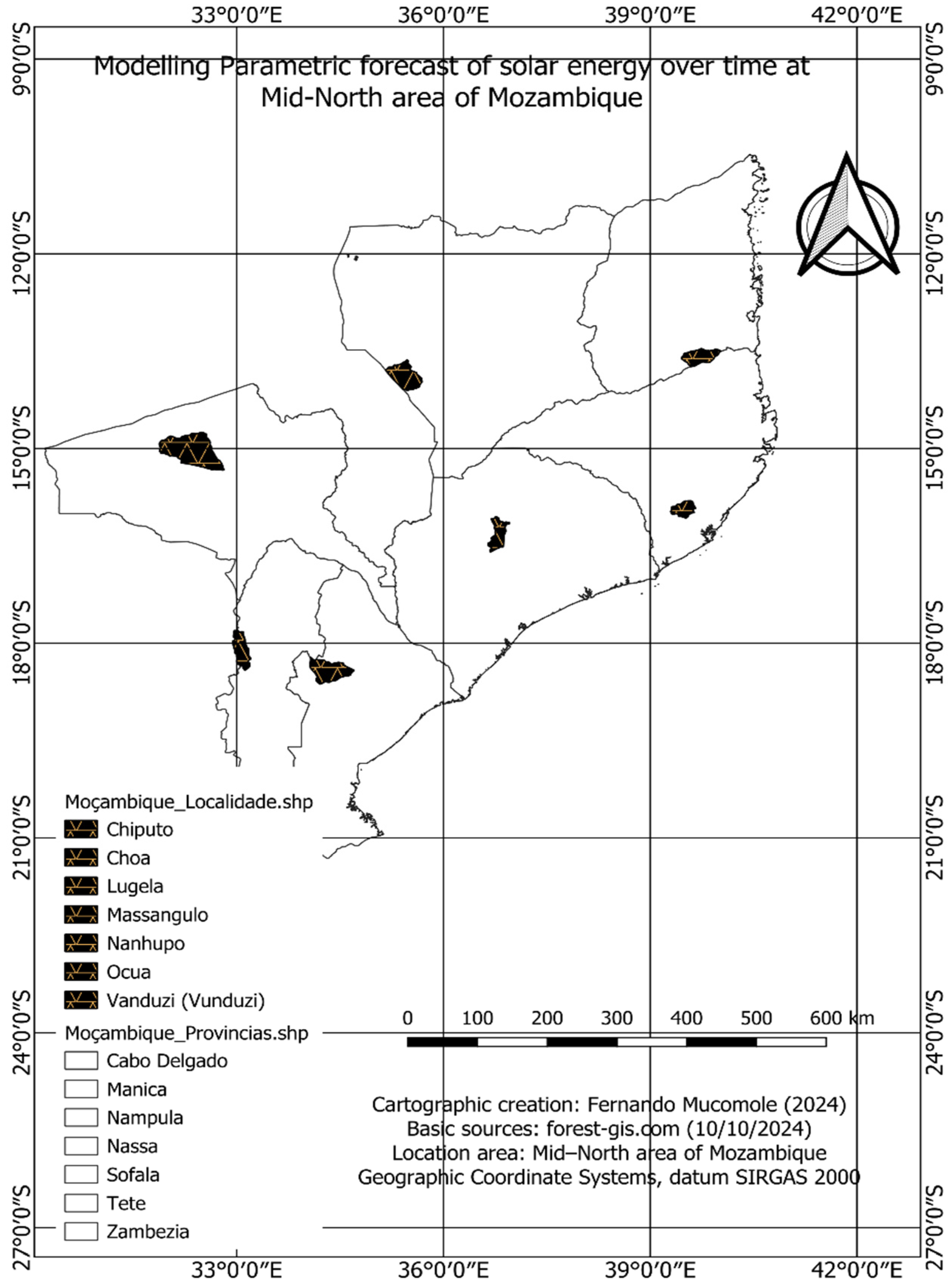
The GHI data sample was obtained during the solar radiation measurement campaign conducted by the National Energy Fund (FUNAE) [56] in 2019, 2020, and 2021 in the Mid-North region of Mozambique. This encompassed the provinces of Cabo Delgado, Nampula, Niassa, Zambezia, Sofala, Manica, and Tete, specifically in the localities of Ocua (FUNAE–MZ03–Ocua), Nanhupo (FUNAE–MZ24–Nanhupo-1 and FUNAE–MZ24–Nanhupo-2), Massangulo (FUNAE–MZ25–Massangulo-1 and FUNAE–MZ25–Massangulo-2), Lugela (FUNAE–MZ32–Lugela-1 and FUNAE–MZ32–Lugela-2), Vanduzi (FUNAE–MZ11–Vanduzi), Choa (FUNAE–MZ21–Choa-1 and FUNAE–MZ21–Choa-2), and Chiputo (FUNAE–MZ06–Chiputo). The arrangement included two measurement stations each in Nanhupo, Massangulo, Lugela, and Choa (so, two stations at each location), and single measuring stations in Vanduzi, Chiputo, and Ocua, resulting in a total of eleven high-resolution radiometers. These radiometers were positioned at distances greater than 1000 km (specifically 1060.6 km, 1510.5 km, 1632.8 km, 1799.56 km, 1952.5 km, 2056.9 km, 2145.5 km, 2298.1 km, 2455.7 km, 2608.4 km, and 2789.5 km), as illustrated in Figure 1.

Figure 1 also shows the correlational behaviors of the stations in the mid-north region about the other measurement stations of the campaign in other regions of Mozambique, depending on the distance from the Indian Ocean to Zumbo; it can be seen that they present a positive dependence relationship with trips through the mid-north region.

The GHI and DHI radiation components were measured using PY 5886 pyranometer radiometer sensors (produced by NRG Systems, in Houston, TX, USA) with the behavior shown in Figure 2, which were connected to a system that included an inserted pyrheliometer that directly determined the DNI component. The pyrheliometer used for data collection was optimized for protection with the following settings: location factor 295–2800 nm, spectral range with a 1-min response, linearity ±0.5%, and cosine ±1%.

After quality control and the removal of erroneous values, the data were processed using programs created especially for calculating radiation at intervals of 10 min.

The Aerosol Robotic Network (AERONET) [57] database provided the validated sample of measurements using the AERONET instrument (sun photometer number 118) to assess the aerosol optical thickness (AOT) at wavelengths of interest. The results are calibrated with the help of developed algorithms, covering measurements along the mid-north regions in the provinces of Niassa (Niassa station) and Sofala (Gorongoza station), at the coordinates shown in

Table 1. Coordinates of the measuring stations.

ID	Site Name	Province	Property	λ (nm)	Amplitude	Level	Long. (°)	Lat. (°)	A (m)
1_A	Niassa	Niassa	AERONET	400–500	4″, 1 and 24 h	2.0	37.5665	−12.155	510
3_A	Gorongoza	Sofala	AERONET	400–500	4″, 1 and 24 h	2.0	37.5665	−12.155	510

. The measurements were conducted from 19 June 2019 to 31 December 2021, with short-scale measurement intervals of roughly 4 min, 1 hour, and 1 day, as well as monthly averages. These data have several levels from levels 1 and 1.5. Nevertheless, we operated them at level 2.0 to achieve improved accuracy, updated processing, and the removal of extra anomalies. This also enabled us to gather data samples for all stations of the collected data, including pressure, precipitation, ozone, Rayleigh scattering, Mie effect, temperature, cloud cover, latitude, longitude, and altitude.

Each instrument was subjected to routine seasonal maintenance during the measurements, including data transmission, battery changes, cleaning, and realignment. Cleaning and orientation periods were recorded during this procedure, except for data selection periods involving turbulence and interference.

For each measurement station, the collected sample (consisting of GHI, pressure, precipitable water, aerosol optical thickness (AOT), ozone layer, uniformly mixed gases, temperature, optical air mass, and zenithal angle) was cleaned and interpolated for missing values at intervals of one and five minutes. The data (e.g., temporal series, as well as atmospheric, spatial, and geographic data disposed of) were then organized into a tab. As illustrated in the second step of the statistical design of Figure 3, the ideal parameters were chosen and tested for the previously mentioned conditions, and ‘good behavior’ was chosen and analyzed as an input in MLM. The clear-sky index, or the ratio of the predicted value to the theoretical clear-sky global solar radiation, was then calculated.

The model’s selection and validation were based on the best possible output relative to the solar constant average and the best possible estimation of every variable fitting the theoretical spectral sun irradiation. The model was verified using the sample that was gathered, and the representative clear sky was analyzed to provide the best forecasting of solar energy for a horizontal surface. As the final phase in Figure 3 illustrates, meta-analyses were carried out using a parametric model to assess the various transmittance levels, irradiances, clear-sky behaviors, and space and time factors.

Throughout the week-long study, the voltage angle was adequately marked each time an inaccurate data calibration was discovered; however, this was not a common occurrence.

2.2. Study Area

Mid-north Mozambique is the study region. It is situated between the meridians 30°12 and 40°51′ east longitude and the parallels 10°27′ and 26°52′ south latitude. This is where the stations (MZ06–Chiputo, MZ11–Vanduzi and MZ21–Choa, MZ32–Lugela, MZ25–Massangulo, MZ24–Nanhupo, and MZ03–Ocua) were installed. Their latitude and longitude characteristics are listed in

Table 2. Locations of study stations campaign.

ID	Station	Province	Tower	Code	Longitude (X)	Latitude (Y)
MZ03	MZ03_Ocua	Cabo Delgado	FUNAE	TM3	39°23’37.17″ E	11°32′58.09″ S
MZ06	MZ06_Chiputo	Tete	FUNAE	TM6	31°40′40.59″ E	14°58′29.18″ S
MZ11	MZ11_Vanduzi	Sofala	FUNAE	TM11	35°2′21.44″ E	19°43′47.70″ S
MZ21	MZ21_Choa	Manica	MceL 1	MCeL 14	33°13′10.22″ E	17°47′33.62″ S
MZ24	MZ24_Nanhupo	Nampula	MCeL 1	MCeL 23	39°30′52.44″ E	15°57′58.42″ S
MZ25	MZ25_Massangulo	Niassa	TDM 2	TDM	35°26′13.56″ E	13°54′28.94″ S
MZ32	MZ32_Lugela	Zambezia	MceL 1	MCeL 44	36°42′48.98″ E	16°28′52.09″ S

where ¹ MceL—stands for Mozambique cellular, ² TDM—telecommunications of Mozambique.

.

The topographic section of the Mid-North region, illustrating the measuring stations, is shown in Figure 4.

As the sun rose and set (between 6:00 and 18:00), the sample was prepared to facilitate the computations using the data from the MZ06–Tete–Chiputo, MZ11–Sofala–Vanduzi, MZ21–Manica–Choa, MZ32–Zambezia–Lugela, MZ25–Niassa–Massangulo, MZ24–Nanhupo, and MZ03–Cabo–Delgado–Ocua campaigns. For the FUNAE and INAM data campaigns, with the samples obtained at the stations comprising intervals of three years of complete measurements (2019, 2020, and 2021), starting in the sixth month of the year, the data covered only the months of June to December; in 2020 and 2021, the data covered all months of the year of complete measurements, totaling approximately 823,478.00 daily radiation data points each in the study’s useful area.

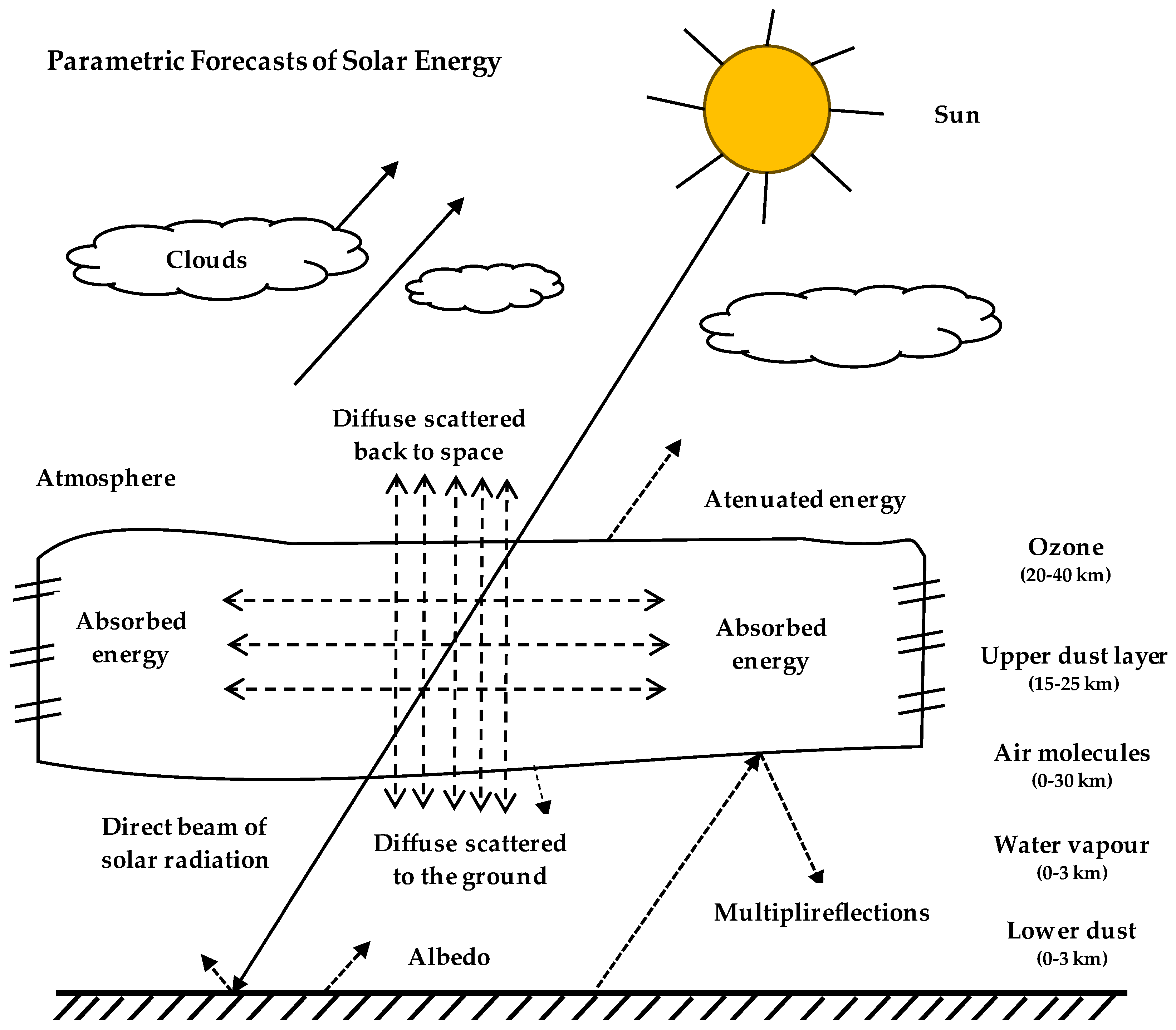
2.3. Solar Radiation Path Above the Surface of the Earth

The path of solar radiation is such that when it reaches the Earth’s atmosphere, some of the incident energy is absorbed by atmospheric layer particles through interactions, and some are scattered away [3,4,6,7,8,9]. Both significantly alter the spectral energy that travels through the atmosphere and have an impact on the alien spectrum, as shown in Figure 5.

As illustrated in Figure 5, diffuse radiation is made up of scattered radiation that returns to space after partially reaching the ground [10,14,19]. Direct radiation, often known as a beam, is the portion of radiation that strikes the earth directly in line with the solar disk. A beam of solar radiation may experience a variety of physical phenomena during this process [3,17], including direct solar radiation scattering, air molecule scattering by Rayleigh, water vapor and solid particle scattering by Mie, Angstrom turbidity for aerosols, direct transmittance owing to continuous attenuation, direct solar radiation absorption by gases, transmittances of molecular absorbers, ozone transmittance, transmittance of uniformly mixed gases and water vapor, and direct spectral irradiance on the ground [5,15,20,21,22,23,24,25,26,27,28,29]. The multiplied reflected spectral diffuse irradiance, diffuse spectral irradiance on the ground, and global spectral irradiance on the ground are all influenced by atmospheric albedo [9,44,56].

2.4. Review of Previous Works

According to the current scenario, the number of people with access to electrical energy increased by 109 million in 2023 (which translates to an annual population increase of 80 million) [10,12,33,36]. Central and Southern Asia saw the largest increase, growing to 51 million [10] up from 24 million people [10,33], followed by Sub-Saharan Africa [10], which saw an annual population increase of about 23% [33] with access, which is in contrast to its annual population increase of about 28 million people [15]. Between the annual population growth and the 2 million additional people who have access to energy, lower rates are seen [16,19,23]. The need for increased adoption of environmentally friendly technology and more seamless energy transitions is closely tied to these figures [10,17]. Being aware of the available solar resources directly impacts renewable energy-generating resources of all sizes [8,12,58].

A forecast of solar energy resources shows how solar energy can be used to its fullest potential and how it will actually be able to create electricity in a solar plant without oscillation, extending its longevity and durability, among other things [15,30,33]. The availability of this resource is affected by several atmospheric factors [1], and needs to be carefully considered; yet, forecasting techniques [3,4], which fall into the following categories, are useful substitutes for knowing the amount of solar energy that is available. Techniques include physical models, suggesting that the phenomenon’s natural decoherence should be taken into account [59,60], statistical models that use static order parameters to account for solar energy [61,62,63], hybrid models that consider the union of models cross-sectionally for larger estimation deficits [9,17,64], and machine learning models that use initial value problems and hybrid problems and considerably reduce the estimation errors. Above all, solar energy forecasting [38,65,66] can be done mainly by sight and is separated into three times: a very short time, which allows the variability parameter to be observed at a shorter resolution [12,33,67]; a short time, which includes even smaller estimates [29,68], a long–short time, which includes both short- and long-term medication measurements [31,69]; and now-casting, which forecasts radiation behavior based on behavior that has been recorded while taking into account other factors that affect the measurement [70,71,72]. Estimation certainty is significantly increased by utilizing MLM [22,38,73] to summarize and output estimates of solar energy based on atmospheric, meteorological, geographical, temporal, and geographic data [1,33,51,74].

In addition to this, current research analyzing a multilayer perceptron approach utilizing artificial neural networks (ANNs) was examined for GHI estimation, yielding error rates of 19.35% and 18.65%, which are considered commendable for this time frame [12,38,39,40,41,42,43,75,76]. Various MLMs were assessed, with ANN models generally providing the most favorable results during both the development and testing phases, exhibiting error values ranging from 3.9% to 13.8% [4,40,77,78]. Additionally, research on the temporal variability of solar energy availability concluded that clear-sky $\left(K_t^{*}\right)$ values fluctuate between their minimum in July and maximum in December [8,79,80,81,82]. Forecasts of solar radiation fluxes for solar power system applications were conducted using multiple linear regression (MLR) and correlation analysis, revealing that the models accurately predict GHI fluxes with a minimal relative error range [49,83,84,85,86,87]. In terms of electricity consumption predictions, various models were compared, demonstrating their effectiveness as alternatives to the stepwise regression model for understanding and forecasting energy consumption patterns [6,7,46,88,89,90]. GHI modeling for any location on Earth was achieved through regression analysis, with the resulting models outperforming existing ones in predicting GHI [20,44,45,64,91,92]. Numerous models are created for the analysis of predicted solar energy; these models can be created empirically, softly, or by simulation [6,7,15,46,47], and are used to calculate the outcomes of green purchasing behavior and government actions [14,16], to model the elements affecting customer attitudes toward solar energy product [1,33,48,49,50]. Apart from the aforementioned issues, the majority of solar energy databases that have been verified and made accessible provide unprocessed data with an emphasis on precision [4,5,33,54,93]. Additionally, the data are better estimated because they share benefits from the same cloud and are affected by the same atmospheric circulation patterns [5,54].

Fossil fuels account for about 37% (plus 11% coal and 16% natural gas) of the energy demand in the energy production scenario [1,10,51,94]. Other energy sources, such as electrification, hydro, wind, and other energy sources, coincidentally require a larger investment, and occasionally the need to destroy the ecosystem [33,95,96], as well as the diversion of water courses, make up about 50% (plus 8% traditional gas, 3% modern biomass, and 3% district heat) [59,97,98] of the energy production scenario. In the energy transition scenario, PV power, an abundant, clean, sustainable, and abundant source [2,10,33,36], accounts for about 22% [10,12], with growth potential in several parts of the world.

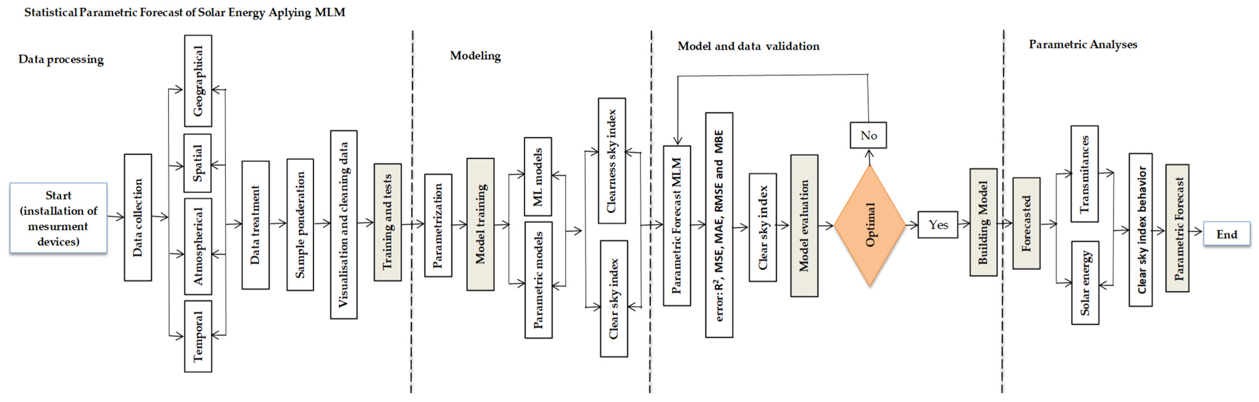
2.5. Experimental Procedure

A sample of meteorological, spatiotemporal, and geographic predictor factors chosen and extracted from the database for solar energy forecast was also made available for verification, along with the GHI data sample that was taken from the Logger database. Equation (1) was utilized in conjunction with observation methods, and measurement tools, and scaled to produce leveled measurement data. They were handled beforehand to reduce losses resulting from potential errors, also known as uncertainty or the margin of error (Error) [33].

$$e=\sqrt{e_a+e_e+e_c}$$

(1)

The formula for calculating $e_a$ is $e_a={\displaystyle \frac{E.S}{\sqrt{n}}}$, where $S$ is the sample’s typical deviation and $E$ is a parameter that depends on the confidence or reliability level $\left(P_k\right)$ selected (typically, it is chosen between 0.90, 0.95, 0.99, or 0.999). Additionally, $e_e$ represents the scale error and $e_c$ is the calibration error that is linked to the instrument’s calibration level and is supplied by the manufacturer.

Forecasting solar energy during the hours of sunlight, or from sunrise to sunset, is crucial for harnessing solar energy. This is because solar modules generate a large amount of solar energy during this time, which can be stored in storage systems or, if needed, injected into the grid. Several issues, including human activity, the demands of birds that obstruct readings, the shading of pyranometers, and the reduction in convectional energy for devices that run on local energy, are among the reasons that the research reveals some days had insufficient data.

Nevertheless, these data gaps were closed using a variety of methods, including data filling interpolation and corrections, as well as with the comparative assistance of measurement installations gathered at FUNAE, INAM, and AERONET. According to data testing, the short-term daily rate has a binomial distribution, which allows the model to be adjusted to the radiation development under clear skies as well as to the theoretical radiation predicted under skies with few clouds, particularly on days with high solar energy incidence. The sample was divided into classes based on the amplitude of oscillations ${At=L}_i-l_i$, and the midpoints or centers of the class ($x_i$ or $P_m$). The sample’s simple absolute frequency, or the number of times or information confirmed in each class, was calculated ($f_{ri}$). This is based on the assumption that $\sum _{i=1}^n{f}_{ri}=1$, and is expressed as a percentage by $f_{r_i}\%=f_{r_i}x100$. We were also able to ascertain the arithmetic mean by numerical analysis [1,33,99]. The block diagram was constructed to better explain the behavior of solar energy for the distribution of the GHI sample, $GHI=\left\{{GHI}_1, {GHI}_2,\dots ,{GHI}_n\right\}$, under the constraint ${GHI}_{i1}\le {GHI}_{i2}\le ,\dots \le {GHI}_{in}$ with the quartiles, in all months of the year.

The radiation analyzed as the minimum in winter and maximum in summer through the box plot was estimated for the daily course of its declination for n days, for the northern (and southern) hemispheres [51,52]. The position relative to the sun for horizontal surfaces is as follows: ${\theta }_Z={90}^0$ results in ${\omega }_s$, is ${\omega }_s={\cos }^{-1}\left(-\tan \varphi \tan \delta \right)$ [3,48]. The corresponding difference in minutes for conversions between solar time and standard time, [3,100], is guided by the eccentricity correction factor of the Earth’s orbit, as provided in Equation (2) [1,52]:

$$E_0=1+0.033\cos \left(n{\displaystyle \frac{360}{365}}\right)$$

(2)

The temporal behavior of the eccentricity correction factor of the Earth is shown in Figure 6, decreasing to the middle year and then increasing to the end along the year time.

Considering the zenith angle, and the idealized parameterization approach [1,3,16,33], the total (spectrally integrated) amount of incident radiation was computed under specified atmospheric conditions, accounting for the radiant energy. The total transmittance of the atmosphere is determined by using regression analysis, as a function of the ozone layer thickness, precipitable water $w$, turbidity parameters $\beta$ and $\alpha$, and air mass $m$. An overall spectrally integrated transmittance for each atmospheric constituent is used in this calculation, as given in Equation (3) [1,3,91]:

$$\zeta =f\left(l,w,\beta ,\alpha ,m\right)$$

(3)

The relative optical air mass $m_{\tau }$, considering air density, and refractive index at wavelength $0.7 \mathsf{\mu }\mathrm{m}$, is given in Equation (4) [1],

$$m_{\tau }={\displaystyle \frac{1}{\left[\cos \left({\theta }_z\right)+0.15{\left(93.885-{\theta }_z\right)}^{-1.253}\right]}}$$

(4)

Considering $p$ as the pressure in mbars, the relative optical mass of the air is denoted as $m_a$. Precipitable water is denoted as $w’$, considering temperature as $T$, the reduce of $w’$ to datum condition, is given as $w=w^{\prime }{\left({\displaystyle \frac{p}{1013.25}}\right)}^{{\displaystyle \frac{3}{4}}}{\left({\displaystyle \frac{273}{T}}\right)}^{{\displaystyle \frac{1}{2}}}$ [3,48,52].

The thickest vertical ozone layer, represented in centimeters by $l$, is the relative optical path length of ozone $U_3$, where $U_3=l{m}_{\tau }$. $U_1=w{m}_{\tau }$ is the relative optical path length adjusted for precipitable water pressure [69,101,102]. Assuming a multiplicative transmittance of multiplicative $\zeta =\prod _{i=1}^{i=j}{\zeta }_i$. In order to illustrate the transmittance via Rayleigh scattering, ${\zeta }_r$, the distinct spectrally integrated quantities of the direct irradiance owing to the different atmospheric elements, given in Equation (5), are as follows [51,69,103],

$${\zeta }_r=exp\left[-0.0903\left(m_a^{0.84}+m_a^{1.84}-m_a^{1.85}\right)\right]$$

(5)

Using ${\zeta }_0=1-{\alpha }_0$ [1], one may determine the transmittance for direct irradiance owing to ozone absorption, or ${\zeta }_0$, as given in Equation (6) [52,74,104]:

$${\zeta }_0=1-\left[{0.1611U_3\left(1.01+139.48U_3\right)}^{-0.3035}-0.002715U_3{\left(1.0+0.044U_3+0.0003U_3^2\right)}^{-1}\right]$$

(6)

The transmittance for uniformly mixed gas absorption under direct irradiance, ${\zeta }_g$, deposited over space and time in the atmospherical medium, is expressed in Equation (7) [3,51]:

$${\zeta }_g=exp\left(-0.0127m_a^{0.26}\right)$$

(7)

The transmittance for direct radiation caused by water vapor absorption ${\zeta }_w=1-{\alpha }_w$, represented by ${\zeta }_w$, as given in Equation (8) is as follows [1,66,105,106]:

$${\zeta }_w=1-{\displaystyle \frac{2.4959 U_1}{\left[{\left(1.01+79.034.U_1\right)}^{0.6828}+6.385U_1\right]}}$$

(8)

The transmittance for direct irradiance owing to aerosol attenuation is denoted by ${\zeta }_a$, considering variation ${\delta }_a$ as ${\delta }_a=0.28{\delta }_{a1}+0.35{\delta }_{a2}$, is given as Equation (9) [1,107]:

$${\zeta }_a=exp\left[-{m_a}^{0.91708}\left({{\delta }_a}^{0.873}+{{\delta }_a}^{1.873}-{{\delta }_a}^{1.5818}\right)\right]$$

(9)

The direct normal irradiance, consisting in the direct incident beam of solar radiation is presented in Equation (10) as [2,16,33]:

$$G_b=G_n.\cos {\theta }_z$$

(10)

The transmittance of direct radiation due to aerosol absorption ${\zeta }_{aa}$, is given in Equation (11) [51,108]:

$${\zeta }_{aa}=1-\left(1-w_0\right)\left(1-m_a+{m_a}^{1.06}\right)\left(1-{\zeta }_a\right)$$

(11)

The scattered diffuse Rayleigh irradiance, caused by interaction of solar radiation and very small particles, that can scatter over space during the daily time, is given in Equation (12) [1,3,48]:

$$G_{dr}=0.395G_{sc}{\displaystyle \frac{\cos {\theta }_z{ \zeta }_0{\zeta }_g{\zeta }_w{\zeta }_{aa}\left(1-{\zeta }_r\right)}{\left(1-m_a+{m_a}^{1.02}\right)}}$$

(12)

Summary transmittance, resulting as fraction of incident energy transmitted after scattering effect of aerosols, as given in Equation (13), as follows [4,12]:

$${\zeta }_{as}={\displaystyle \frac{{\zeta }_a}{1-\left(1-w_0\right)\left(1-m_a+{m_a}^{1.06}\right)\left(1-{\zeta }_a\right)}}$$

(13)

Diffuse irradiance scattered by aerosol, as given in Equation (14), is as follows [1,52]:

$$G_{da}=0.79G_{sc}{\displaystyle \frac{\cos {\theta }_z{\zeta }_0{\zeta }_g{\zeta }_w{\zeta }_{aa}.F_c\left(1-{\zeta }_{as}\right)}{\left(1-m_a+{m_a}^{1.02}\right)}}$$

(14)

Multiple reflected radiation, resulting from the ground and upper atmospheric layer reflections of incident solar energy on a multi-scale level, is presented in Equation (15) as [1,51,52]:

$$G_{dm}={\displaystyle \frac{\left(G_n\cos {\theta }_z+G_{dr}+G_{da}\right){\rho }_g{\rho }_a^{\prime }}{1-{\rho }_g{\rho }_a^{\prime }}}$$

(15)

Global radiation, which consists of the sum of all components of solar radiation, is presented in Equation (16) as follows [3,8,33]:

$$G=G_b+G_d$$

(16)

Data were taken from the original, in situ measurements. The corresponding measurement errors were then found by applying models for forecasting solar energy data. Most of the models under consideration are MLM-built using cutting-edge artificial intelligence techniques, specifically, the Random Forest model is used to search for weather stations by creating three neighborhoods with varying sizes. The spatial dataset is defined as $GHI$, and the neighborhood surrounding station o is denoted as $N_0^k$, where $d(0,i)$ and, $j_k$ represent the distance and weighted average, as given in Equation (17) [109,110]:

$$\overline{G}\left(N_0^k\right)=\sum _{G_i{N}_0^k}{\lambda }_i{GHI}_i$$

(17)

where ${\lambda }_i={\displaystyle \frac{d_{i0}^{-r}}{\sum _{z_i{N}_0^k}{d}_{i0}^{-r}}}$ [111,112] measures the relative inverse distance weights between stations, $r$ is the specified exponent parameter that amplifies the relevance of nearest neighbors [113,114]. Utilize the Regression Kriging (RK) model, which combines anticipated regression trends with anticipated Kriging residuals provided, as given in Equation (18) by [115]:

$$\widehat{G}\left({GHI}_0\right)=\sum _{k=0}^p{\widehat{\beta }}_k{q}_k\left({GHI}_0\right)+\sum _{i=1}^m{\widehat{w}}_{i}e\left({GHI}_i\right)$$

(18)

Here ${\widehat{\beta }}_k,(with k=0, 1, \dots , p)$ denote the Kriging weights, where $p$ is the number of auxiliary variables, $q_0\left(x_0\right)=1$ is a constant term [115,116], the residual is denoted by $\widehat{e}\left(x_0\right)$. With continuous variables $y$ and $x$, simple linear regression (SLR) was trained for values $\left(x_i,y_i\right)=1, \dots ,n$, and provided as given in Equation (19) by [3,50,117]:

$$G={\beta }_0+{\beta }_1{GHI}_i+{\epsilon }_i$$

(19)

Since $E\left({\epsilon }_i\right)=0, Var\left({\epsilon }_i\right)={\sigma }^2$, and ${\epsilon }_i~N\left(0,{\sigma }^2\right)$, the errors ε₁, …, ε_n are all identically independent. The regression line represents the estimate $\widehat{f}\left(GHI\right)={\widehat{\beta }}_0+{\widehat{\beta }}_{1}GHI$, which is provided as $\widehat{E\left(\left.y\right|x\right)}$ for the expected value of the condition $\widehat{y}={\widehat{\beta }}_0+{\widehat{\beta }}_{1}GHI$ [117,118]. The artificial neural network (ANN) model was applied, taking into account an input range of $u_i$ to $u_n$ for each neuron $j$. This range is then multiplied by the weights $w_{ij}$, gathered in neuron $j$, and provided by Equation (20) [32,119]:

$$G_j=\sum _{i=1}^n{w}_j{u}_j+w_{0j}$$

(20)

where $w_{0j}$ is included and calls itself. The activation function is applied to the value $S_j$ given by $f\left(GHI\right)={\displaystyle \frac{1}{1+e^{-GHI}}}$ [32,120]. A Support Vector Machine (SVM) is used, which might be regular, binomial, or Poisson, in opposition to a linear or simple exponential regression, where the sample has a normal distribution and linear space, as given in Equation (21) [103,121]:

$${min}_{w,b,{\varnothing }_i}{\displaystyle \frac{1}{2}}{\left|\right|w\left|\right|}^2+C\sum _{i=1}^n{\varnothing }_i$$

(21)

When is subjected to $y_i\left(w^T+b\right)\ge 1-{\varnothing }_i$, the weight vector and bias are denoted by w and $b,$ C is the regularization parameter, and ${\varnothing }_i$ are the slack variables [64,73]. In order to comprehend or forecast the upcoming time series, we characterize the variables as a linear combination using the ARIMA Model (Autoregressive Integrated Moving Average), as given in Equation (22) [122,123,124]:

$$\mathsf{\varphi }\left(L\right)X_t=\Theta \left(L\right){\epsilon }_t$$

(22)

Here $\mathsf{\varphi }\left(L\right)$ is the autoregressive (AR) polynomial, $\Theta \left(L\right)$ is the moving average (MA) polynomial and ${\epsilon }_t$ represents the error term [123,125,126]. Regression classification is done using a model called Gradient Boosting Machines (GBMs). It builds a forecasting model by combining decision trees. When we take into account regression values, $\eta$ is the learning rate, $h_m\left(GHI\right)$ is the prediction function of the model in the m-th iteration, the forecast for the initial prediction $F_0\left(GHI\right)$, gives the model as in Equation (23) [65]:

$${\widehat{G}}_i=F_0\left({GHI}_i\right)+\sum _{m=1}^M\eta h_m\left(GHI\right)$$

(23)

One effective nonparametric Bayesian regression method for modeling intricate interactions in data is the Gaussian Process Regression (GPR) method. As a prior over functions, it assumes a Gaussian process, as given in Equation (24) [1,88]:

$${\mathit{f}}_{\mathit{*}}|\mathit{G}\mathit{H}\mathit{I},\mathit{y},{\mathit{G}\mathit{H}\mathit{I}}_{\mathit{*}}~\mathcal{N}\left({\mathit{\mu }}_{\mathit{*}},{\sum }_{\mathit{*}}\right)$$

(24)

where ${\mathit{f}}_{\mathit{*}}$ are the predicted values, $\mathit{G}\mathit{H}\mathit{I}$ are the observed input points, $\mathit{y}$ are the observed target values, ${\mathit{G}\mathit{H}\mathit{I}}_{\mathit{*}}$ are the new test points where predictions are to be made, ${\mathit{\mu }}_{\mathit{*}}$ is the mean of the predictive distribution, and ${\sum }_{\mathit{*}}$ is the covariance (or variance) of the predictive distribution. A series of recurrent neural networks (RNNs) with Long Short-Term Memory (LSTM) are used to learn and predict datasets. The forget gate, hidden state output, and cell state memory are crucial for accurate prediction, as given in Equation (25) [17,127]:

$$f_t=\sigma \left(sigmoid\left(W_f{h}_{t-1}+W_f^{\prime }{GHI}_t+b_f\right)\right)$$

(25)

Considering $W_f$ and $W_f^{\prime }$ are the weight matrices for the hidden state $h_{t-1}$ and the input ${GHI}_t$, $\sigma$ is the sigmoid activation function, and $b_f$ is the bias term.

The input gate (i_t) determines which part has the least amount of information. The clear-sky index $K_t^{\mathrm{*}}$ relates GHI to clear-sky radiation, as given in Equation (26) [1,2]:

$$K_t^{\mathrm{*}}={\displaystyle \frac{GHI}{G_{Clear}}}$$

(26)

Consider $G_{Clear}$, as the total radiation. According to the statistical analysis, the median which divides an increasing or decreasing set into two equal portions, 50% and 50% was found in each of the 11 measurement sites. For odd-numbered elements, even-numbered elements, and data divided into classes, we have values that precede the 25% of the frequency below it, known as the first quartile (Q₁), the second quartile (Q₂) is equal to the median value, and the third quartile (Q₃) is the value that precedes the 75% of the frequency almost below the one that follows the 25%. The mode or norm (M_o) and the separatrix were found. The interquartile interval was analyzed. After estimating the variability measures, a mean deviation and standard deviation were found. Taking values of $K_t^{*}$ for different classes of days (clear, intermediate and cloudy) a connection was made as a function of the distance of the correlation coefficient or systematic connection of the clear-sky index ${\chi }_{ij}^{k_t^{*}}$, as given in Equation (27) [3,128]:

$${\chi }_{ij}^{k_t^{*}}={\displaystyle \frac{cov\left(∆k_{\tau ,i}^{*}\left(t\right),∆k_{\tau ,j}^{*}\right)}{{\sigma }_{∆k_{\tau ,i}^{*}\left(t\right)}{\sigma }_{∆k_{\tau ,j}^{*}}}}$$

(27)

Statistically, ${\chi }_{ij}^{k_t^{*}}$ varies spatially from −1 to 1, considering for a subspace station between two points $x$ and $y$, randomized values relates to $x+y$, with ${\sigma }_{∆k_{\tau ,i}^{*}\left(t\right)}\ne 0 and {\sigma }_{∆k_{\tau ,j}^{*}}\ne 0$ [33,61,128].

3. Results

3.1. Evolution of the Solar Energy Characteristics in Terms of Space and Time

The plateau plains of Mozambique’s Mid and Northern regions are typically 20 m above sea level. However, there are also mountains at an elevation of approximately 5400 m that support a range of activities, from small-scale emissions to contributions to the atmosphere, such as aerosols released by natural activities like emissions from the sea, industrial burning, gases, and fixed particles from industrial combustion and mining, though the heavy area exploration industry makes a significant contribution.

In contrast to the North, Figure 7 illustrates how human and industrial activity, in the Mid region, caused a higher aerosol deposition in the Mid area, with a bigger concentration of optical thickness of aerosols at both wavelengths of 675 nm and 440 nm. For the first, however, a larger concentration of these was seen in 2021, with a maximum of 0.5821 and a minimum of 0.0248, in the range of 0.2351, with a deviation of 0.1309. However, because of various activities, a reduction in this concentration was seen in 2020, averaging approximately 0.1798 with a variation of 0.1576 (a maximum of 0.6130 and minimum of 0.0361). Its concentration in 2019 was predicted to be 0.2060 with a 0.1576 deviation (with the highest being 0.8769 and minimum being 0.0325), which indicates that it remained high. However, 0.3478 was observed with a deviation of 0.2172 (maximum of 0.9656 and minimum of 0.0178) for wavelengths of the order of 440 nm, in contrast to the intermediate levels of reduction seen by the existence of multiple mitigation and capture projects for these resources and the local sensitization estimated at around 0.3160 with a deviation of 0.2018 (with a maximum of 0.9382 and minimum of 0.0545).

The aerosol population for light observation under wavelength 675 nm in the North, illustrated in Figure 8 increased to 0.1579 in 2021, presenting a deviation of 0.0766 (with maximum values of 0.0335 and 0.5309), in contrast to the 0.1515 observed in 2020 with a deviation of 0.0794 (with an observed maximum of 0.5572 and minimum of 0.0392).

Industrial activity, however, was introduced in 2019, and mostly led to a low optical thickness, with an optical thickness of 0.1230 and a deviation of 0.0948 (with a maximum of 0.5090 and a minimum of 0.0227). In 2020, an analogous analysis was verified for light with wavelengths of 440 nm. The aerosol concentration thickness varied by 0.13992, reaching a maximum of 0.7413 and a minimum of 0.0427.

Higher precipitable water concentrations were recorded in the Mid region in 2020, estimated at 2.6898 cm with a deviation of 0.717 cm (reaching from 1.3856 cm to 4.5200 cm), and in 2019 at 2.6613 cm with a deviation of 0.7940 cm (from 1.2439 cm to 4.6395 cm). In 2021, the minimum precipitable water thickness was recorded at approximately 2.5927 cm with a deviation of 0.5882 cm (from 1.3205 cm to 4.3521 cm), shown in Figure 9a.

The highest concentrations, however, were recorded in 2021 with a deviation of 0.8917 cm (from 1.1347 cm to 5.2506 cm) and 2.7061 cm in 2019 with a deviation of 0.8844 cm (from 1.3714 cm to 5.2863 cm). However, there was a decrease of approximately 2.2767 cm with a deviation of 0.6479 cm (from 4.5303 cm to 1.0454 cm) in the Mid region. This is because there is a tendency for precipitable water to decline in both regions, with a focus on the current years impacted by the uneven distribution of solar radiation and its reduction that endangers the hydrological cycle’s frequency of rotation.

The North region’s fluid pressure in the cloud is determined by small-scale atmospheric circulations, and in 2019 it was estimated to be as low as 960.6477 mbars with a deviation of 1.8290 mbars (from 958.1009 mbars to 963.0724 mbars). However, in 2021, pressure dropped to 957.1626 mbars with a deviation of 1.4845, with a maximum of 959.5428 mbars and a minimum of 953.3735 mbars, as depicted in Figure 10a.

The Mid region’s high-altitude levels in relation to sea level and local atmospheric circulations were responsible for the high pressures, which were estimated to have reached minimum values of around 1012.9 mbars in 2019 with a deviation of 3.1897 mbars (from 1017.3 mbars to 1006.2 mbars). In 2020, the pressures increased to 1014.3 mbars with a deviation of 5.6937 mbars (from 1001.9 mbars to 1021.01 mbar). Nevertheless, the circulations and the relaxation of emission activity on high scales helped to reach minimum pressures in 2019, with a deviation of 4.9865 mbars (between 1007.3 and 1020.8 mbars).

The ozone layer in the North region is shown in Figure 10b to have been estimated in 2019 at a layer of approximately 2.5460 cm with a deviation of 0.0031 (ranging from 2.5500 to 2.5411), but its thickness increased to 2.6165 in 2020 with a deviation of 0.0080 (ranging from 2.5899 to 2.6263). In 2021, however, it decreased to 2.5989 with a deviation of 0.0066 (ranging from 2.5939 m to 2.6126 cm) as a result of gas circulations caused by low human activity and industrial awareness of carbon capture caused by the cause, combined with the measurement of climatic effects. Greater concentrations of ozone layer gases are found in the mid region. For instance, a thickness of 2.8449 cm was observed in 2021 with a deviation of 0.0437 (maximum of 2.8964 and minimum of 2.7739); however, in 2019 it was estimated at 27470 with a deviation of 0.1082 (from 2.5821 to 2.92131); comparatively less gas deposition was observed by various phenomena in 2020 in the order of thickness of the ozone layer of 2.700 with a deviation of 0.1330 (from 2.5641 to 2.8946), as shown in Figure 9b.

The data presented in Figure 9c indicate that there was a higher deposition of uniformly mixed gases in the mid region. Specifically, NO₂ was estimated to have been present in the order of 0.0015 cm in 2020, with a deviation of 0.00032 cm (from 0.010 cm to 0.0018 cm), and 0.0013 cm in 2019 with a deviation of 0.000019 cm (from 0.0012 cm to 0.0013 cm). In contrast, less accurate estimates of these gases’ concentrations were found in 2021, with a deviation of 0.0000069 cm (from 0.0016 cm to 0.0021 cm).

The impacts of atmospheric turbidity brought on by other atmospheric elements are responsible for the higher amounts of these gases in the Mid area, as seen from the region of Figure 9c. In 2021, there was a decrease in these gases and the NO₂ concentration that was measured in steps of 0.0020 cm, with a variation of 0.00017 cm (high of 0.0021 cm and minimum of 0.0016 cm).

The North experienced temperatures that tended toward extremes due to the various greenhouse gas and climate change factors previously discussed. Maximum average temperatures in 2021 were estimated to be 29.8077 with a deviation of 3.9501 (from 291.700 to 306.8077); however, in 2021 and 2019, an average and vertical temperature of 292 with ma was observed, as shown in Figure 10d. Figure 9d illustrates the significantly higher temperatures in the Mid region. The maximum temperature in 2021 was 302.8754 with a deviation of 5.4748 (from 292.1000 to 312.9000), and in 2020 and 2019, approximately 302.3036 was reached with a deviation of 9.0773 (from 290.600 to 322). In 2019, 302.7691 was reached with a deviation of 5.4748.

The air mass’s optical path along the north region showed, as shown in Figure 9e, minimum values in 2020 of around 1.4200 with a deviation of 0.6823 (1.033 to 4.8829), moderate values in 2021 of around 2.4186 with a deviation of 1.4151 (from 1.1223 to 6.8488), and high values in 2019 of around 2.5516 with a deviation of 1.4390 (from 1.2283 to 6.5383). The air mass, however, exhibited stronger atmospheric resistance in the Mid region; in 2019, the air mass’s optical path was recorded at 2.3855 with a deviation of 1.2638 (from 1.0539 to 6.4721), 2.3266 with a deviation of 1.1910 (1.0614 to 6.4097), and the lowest values were recorded in 2021 at 1.7545 with a deviation of 0.7822 (from 1.0539 to 6.4721).

The zenith solar angle is observed to observe maximums in 2019 around 58.5855 with a deviation of 15.3276 (from 35.5590 to 81.5707), but it decreases in 2020 in the order of 36.7508 with a deviation of 14.3157 (from 4.8521 to 78.4530), and averages in 2021 of around 55.7083 with a deviation of 17.4576 (from 27.0621 to 58.1141). This can be attributed to the optical path that experiences multiple reductions, as shown in Figure 10f. However, Figure 10f shows that there was a decline in the Mid region, with values of 44.9561 with a deviation of 19.5491 in 2021 (from 14.0493 to 75.1894), 55.5144 in 2020 (from 19.6495 to 81.3853), and 57.4773 in 2020.

On the other hand, as illustrated in Figure 11, when all days of the year are examined in each season, there are days when GHI (brown line) is almost exactly following the theoretical radiation path (blue line), which are ideal days, and days when radiation is very far away (the opposite of GHI shown in Figure 11). This is due to several atmospheric phenomena as well as human and animal activity, which makes it impossible for the solar radiation signal to be captured as optimally as possible. Figure 11 shows the annual trend of solar energy collected, with a peak at noon and a trough at dawn and sunset.

In addition to providing excellent trends in the estimation of solar energy, the daily course of energy through a simple linear regression (SLR) illustrates such affinity of daily development, with its estimated values following the daily course. Resulting in a correlation level in the order of 0.989, as can be seen in Figure 12.

In all observed seasons, the pattern of the daily solar radiation pattern is described by the daily and monthly anomalies shown in Figure 13.

But as can be seen, solar energy is highest during the summer and lowest during the winter. This is something to keep in mind when sizing PV systems to ensure maximum development and durability in terms of power projection regarding daily energy consumption, as illustrated in the year-round boxplot of solar energy levels shown in Figure 14.

The annual energy levels, measured in $\mathrm{W}/{\mathrm{m}}^2$, are detailed as follows: In the Cabo Delgado province at Ocua station, the average for 2019 was 280.7, with a peak of 740.31 and a low of 240.5. In 2020, the average increased to 362.61 (369.79 to 463.66). In the Nampula province at the Nanhupo-1 station, the average for 2019 was 419.13 (587.89 to 83.6). The averages for 2020 and 2021 were 360.6 (913.43 to 139.8) and 410.56 (328.48 to 771.6), respectively. At the Nanhupo-2 station, the average for 2019 was 326.35 (543.2 to 76.28). In 2020, the average rose to 378.16 (424.71 to 430.8). In Niassa province at the Massangulo-1 station, the average for 2019 was 442.38 (648.9 to 33.2). In 2020, the annual average was 428.96 (694.01 to 185.3). The average for 2021 was 428.81 (680.4 to 60.3). At the Massangulo-2 station, the average for 2019 was 375.24 (578.5 to 118.9). In 2020, the average decreased to 345.49 (630.1 to 103.1), while in 2021, the average further declined to 288.48 (501.7 to 85.80).

In the Zambezia province, at the Lugela-1 station, the recorded data for the year 2019 indicated an annual average of 957.56 (688.56 to 74.79). In 2020, the average dropped to 40.02 (647.19 to 998.3). For 2021, the average was 392.89 (398.89 to 107.71). Additionally, at the same Lugela-1 station, the average for 2019 was noted as 937.47 (440.40 to 246.6). In 2020, the average was 390.29, maintaining the same maximum and minimum values as the previous year. The year 2021 recorded an average of 367.99, with a maximum of 882.1 and a minimum of 355.2. Furthermore, the on-site collected values indicate a strong correlation with correction levels, achieving a coefficient of 0.9999, as illustrated in

Table 3. Relationship between transmittances and irradiances.

Transmittance						Irradiance
${\mathit{\zeta }}_0{\mathit{\zeta }}_{\mathit{g}}$	${\mathit{\zeta }}_0{\mathit{\zeta }}_{\mathit{w}}$	${\mathit{\zeta }}_0{\mathit{\zeta }}_{\mathit{a}\mathit{s}}$	${\mathit{\zeta }}_0{\mathit{\zeta }}_{\mathit{r}}$	${\mathit{\zeta }}_0{\mathit{\zeta }}_{\mathit{a}}$	${\mathit{\zeta }}_{\mathit{w}}{\mathit{\zeta }}_{\mathit{a}\mathit{a}}$	${\mathit{G}}_{\mathit{n}},{\mathit{G}}_{\mathit{d}\mathit{r}}$	${\mathit{G}}_{\mathit{n}},{\mathit{G}}_{\mathit{d}\mathit{a}}$	${\mathit{G}}_{\mathit{n}},{\mathit{G}}_{\mathit{d}\mathit{m}}$	${\mathit{G}}_{\mathit{n}\mathit{b}},{\mathit{G}}_{\mathit{d}}$
1.000	0.9999	0.9988	1.00	0.9985	0.9981	0.8945	1.000	0.8924	0.9995

.

3.1.1. Examination of Model Performance Inaccuracies

In the order of error assessment based on MAE (W/m²), MAPE (%), RMSE (W/m²), and a coefficient error, R², for the estimated radiation values, a better appreciation and favorable tests were obtained using the ANN and random forest models and their variables in all the considered stations, with a greater focus on the 2020 sample, as an example, in the following provinces: Niassa, at Massangulo-1 station in 2020: ANN errors of 8.52, 4.28, 12.56, 0.89 and RF errors of 10.72, 5.34, 16.84, 0.93, to the detriment of RK errors of 28.12, 12.86, 36.54, 0.38, SVM errors of 28.14, 12.75, 36.52, 0.38, ARIMA errors of 26.18, 11.86, 35.42, 0.46, GBM errors of 26.12, 11.23, 35.12, 0.45, GPR errors of 25.19, 11.12, 35.03, 0.43, LSTM errors of 25.08, 11.01, 34.18, 0.39, and SLR errors of 30.42, 12.01, 35.09, and 0.93.

3.1.2. Examination of the Forecasted Solar Energy at Each Measuring Location

Based on the transmittances of the different air constituents present and the atmospheric parameters used, this led to the development of an estimative behavior differentiating the solar energy that enters the Earth’s surface due to various atmospheric factors that affect the Earth’s unique geometries. This behavior is then noted and evaluated in all analytical states:

At the North Region

In the province of Niassa, at the Massangulo-1 station, Figure 15a shows that in 2020, there was reduced attenuation due to uniformly mixed gases, with an average transmittance of ${\zeta }_g$, of magnitude 0.9873 (0.9868 to 0.9876), and an average ozone ${\zeta }_0$ of 0.9127 (0.9079 to 0.9153). Water vapor absorption exhibited a transmittance of ${\zeta }_w$, averaging 0.9059 (0.9058 to 0.9059). Aerosol attenuation, on the other hand, exhibited a transmittance of ${\zeta }_a$, averaging 0.8538 (0.5362 to 0.9569), whose transmittance, ${\zeta }_{aa}$, demonstrated an average of 0.9927 (0.9775 to 0.9979). The multiplicative transmittance ${\zeta }_t$ exhibited an average of 0.5267 (0.3060 to 0.6103), indicating a reduced Rayleigh scattering effect (${\zeta }_r$) of around 0.0001. The diffuse irradiance $G_g$ presented an average of 112.8236 (40.5337 to 315.3244) on the horizontal surface, as indicated by Figure 15b. This is due to the diffuse irradiance by Rayleigh scattering $G_{dr}$, which presented an average of 0.0001, deviating very little from the diffuse irradiance $G_{da}$, which presented an average of 95.3581 (28.5913 to 287.9701), and the radiance of multiple reflections between the Earth’s surface and its cloudless sky atmosphere $G_{dm}$, which presented an average of 17.4655 (11.9425 to 27.5544). The average irradiance of the experimental sample, $G_{exp.}$, was 514.7994 (202.7880 to 895.8279), while the average irradiance of the theoretical sample, $G_{theor.}$, was 770.2244 (582.5156 to 879.7705). An average of 430.0858 (126.7001 to 694.1001) was found in the measured irradiance GHI. To account for increasing albedo, the irradiance of numerous reflections between the Earth’s surface and its clear-sky atmosphere increased. As an illustration, Figure 15c shows a mean of 17.4655 (11.9425 to 27.5544) for low albedo of order 0.25, and 71.0385 (47.9958 to 114.7522) for 0.95. In contrast to values calculated using only shape variables, Figure 15d illustrates a tendency of more prevalent real values in the solar energy estimated using all characteristic data.

Similar to the analyses made in Figure 15, the minimum attenuation resulting from airborne particles with transmittance for direct irradiance, ${\zeta }_0$, was estimated to be 0.8891 (0.9649 to 0.6423) in 2019. Additionally, 0.907, due to absorption by water vapor, ${\zeta }_w$, deviated to 0.0334. On the other hand, uniformly mixed gases, with ${\zeta }_g$ in the order of 0.9873 (0.9869 to 0.9876), attenuated slightly more than ozone with ${\zeta }_g$ with an average of 0.9127 (0.9088 to 0.9188). Meanwhile, Rayleigh scattering, with ${\zeta }_r$, presented an average of 0.9845 (0.756 to 0.899) and was significant but less contributory in relation to ${\zeta }_{aa}$, with an average of 0.9944 (0.9821 to 0.9955), and the total transmittance, ${\zeta }_t$, presented the generalized estimate with an average of 0.5460 (0.3976 to 0.6088). As we approached the cold and dry seasons, the measured experimental irradiance ($G_{exp.}$) decreased smoothly with an average of 607.2635 (329.0814 to 918.7541). On the other hand, the diffuse irradiance on a horizontal surface fitted within the theoretical irradiance ($G_{theor.}$), and appeared highly defined with an approximate intensity of 872.1686 (690.6895 to 9.72.1477). Rayleigh scattering ($G_{da}$), with an average of 72.8277 (18.7074 to 234.0865), and the attenuation of diffuse irradiance due to multiple reflections between the Earth’s surface and its atmosphere ($G_{dm}$), with an intensive mean of 18.8429 (26.4122 and 12.7760), also contributed to ($G_d$). The irradiance resulting from multiple reflections varied approximately linearly with surface albedo; nevertheless, as surface albedo increased from 0.25 to 0.85, the irradiance resulting from multiple reflections increased.

The minimum attenuation by uniformly mixed gases at the Massangulo-1 station in 2021 showed a transmittance ${\zeta }_g$ of an average magnitude of 0.9873 (0.9868 to 0.9876). A little less attenuated than ozone ${\zeta }_0$, with an average of 0.9129 (0.9091, 0.9081 to 0.9153). The average value of ${\zeta }_r$, or the Rayleigh scattering effect, was 0.9927 (0.9813 to 0.9927), which was comparatively smaller than the average value of ${\zeta }_a$, or the transmittance, which is 0.8547 (0.6263 to 0.9591). The multiplicative transmittance ${\zeta }_t$ had an average of 0.5281 (0.3879 to 0.6127) due to absorption by water vapor with a transmittance ${\zeta }_w$ of 0.9018 (0.908 to 0.9059). The behavior on the horizontal surface showed that the diffuse irradiance $G_d$ had an average of 112.5279 (0.38.6458 to 276.1939), larger than its components due to aerosol-diffused Rayleigh scattering, while $G_{dr}$ had an average of 0.01. Between the Earth’s surface and its clear-sky atmosphere, $G_{dm}$ exhibited an average irradiance under multiple reflections of 17.4605 (11.3613 to 25.3624), while $G_{da}$ had an average of 95.0674 (27.2844 to 250.8315). The theoretical irradiance $G_{theor.}$, which had a mean of 770.3365 (592.3711 to 877.7546), was not far from the estimated experimental irradiance $G_{exp.}$, which had a mean of 502.8378 (187.7513 to 796.8280). A mean of 416.7325 (60.301 to 650.401) was found for the measured irradiance GHI. Increasing albedo is explained by an increase in the irradiance of numerous reflections between the Earth’s surface and cloudless sky atmosphere. It was observed that, as the mean for the low albedo of order 0.25, was 17.4605 (11.3613 to 25.3624) for 0.85 and 71.0054 (565.6570 to 105.8290) for 0.95.

At Massangulo-2 station, the ozone layer experienced less attenuation in 2019 with a transmittance ${\zeta }_0$ evaluated at 0.9137 (0.9058 to 0.9158), while the set of tenuous water vapor had a transmittance ${\zeta }_w$ of 0.9007 (0.9007 to 0.9017). The minimum attenuation observed by uniformly mixed gases in 2019 showed a transmittance ${\zeta }_g$ in the order of 0.9873 (0.9868 to 0.9876). Aerosols absorbed more, with transmittance ${\zeta }_{aa}$ exhibiting an average of 0.9944 (0.9813 to 0.9982), compared to during attenuation, with transmittance ${\zeta }_{aa}$, exhibiting an average of 0.8891 (0.6423 to 0.9649). The Rayleigh scattering effect ${\zeta }_r$ and mie were much smaller, both in the order of 0.0002. In general, the multiplicative transmittance ${\zeta }_t$ attenuated by the average was in the order of 0.5460 (0.3976 to 0.6088). The summer months saw higher values for both direct irradiance $G_b$ and the estimated experimental irradiance $G_{exp.}$, which averaged 544.3097 (292.2472 to 846.7006), which was close to the theoretical irradiance of the $G_{theor}$ model. With a range of 118.901 to 589.100, the measured irradiance GHI displayed an average of 376.3674. Because of Rayleigh scattering, the diffuse irradiance $G_{dr}$ offered an average of 98.5101 (97.3272 to 100.1227), but the diffuse irradiance $G_d$ presented an average of 189.9808 (131.2457 to 357.8895). The average diffuse irradiance ($G_{da}$), resulting from reflections and scattering between aerosols and the surface, was 72.8277 (18.7074 to 234.0865). On the other hand, the irradiance ($G_{dm}$), resulting from multiple reflections between the Earth’s surface and its cloudless sky atmosphere, was of lesser magnitude, averaging 18.6429 (12.7760 to 26.4122). The average irradiance divergence from numerous reflections between the Earth’s surface and cloudless sky atmosphere was larger, with a comparatively higher Earth albedo in the mostly reflective regions, with 0.85 and 0.95; the averages were 42.1347 and 75.5321, respectively.

Uniformly mixed gases with transmittance ${\zeta }_g$ of the average magnitude 0.9873 (0.9868 to 0.9876) exhibited a minimum attenuation in 2020. Ozone, with transmittance ${\zeta }_0$, decreased and attenuated smoothly throughout the year in the order of 0.9127 (0.9079 to 0.9153). Water vapor, with transmittance ${\zeta }_w$ of average magnitude 0.9059 (0.9058 to 0.9059), contributed less than this. When compared to the absorbance of transmittance ${\zeta }_a$ by aerosols, which showed an average of 0.8538 (0.5362 to 0.9569), the attenuation of scattering by aerosols in a given plane was greater than the transmittance ${\zeta }_{aa}$, with an average of 0.9927 (0.9765 to 0.9979). The Rayleigh scattering effect ${\zeta }_r$ was smaller in the order of 0.0001, but the multiplicative transmittance ${\zeta }_t$ displayed an average of 0.5267 (0.3060 to 0.3158). In accordance with the theoretical irradiance of 770.2244 (582.5156 to 879.7705) of roughly 890.2244 (582.5156 to 879.7705), the direct irradiance and the estimated experimental $G_{exp.}$ increased, with minimum values in the winter and maximum in the summer, in the order of 437.4806 (198.3704 to 828.1725). With components stimulated by the Rayleigh scattering $G_{dr}$ of 0.0001, deviating very little from its average, the diffuse irradiance aerosols $G_{da}$ of an average of 95.3581 (28.5913 to 287.9701), and the irradiance from multiple reflections between the Earth’s surface and its cloudless sky atmosphere $G_{dm}$ of 17.4655 (11.9425 to 27.3544), the diffuse irradiance $G_d$ was smaller, on the order of 112.8236 (40.5337 to 315.3244). Averaging from 103.101 to 630.102, the measured irradiance GHI was 345.9084. The behavior on the horizontal surface demonstrates how the irradiance of multiple reflections between the Earth’s surface and its cloudless sky atmosphere increases, taking increasing albedo into consideration. The values are of the order of 17.4555 for an albedo of 0.25, 39.5374 for 0.85, and an average of 71.0385 for 0.95.

A smaller attenuation was caused by uniformly mixed gases of transmittance (${\zeta }_g$) of 0.9873 (0.9868 to 0.9876) in 2021 than by ozone (${\zeta }_0$ of average 0.9129). An even smaller attenuation was caused by water vapor of transmittance (${\zeta }_w$) of 0.9073 (0.9072 to 0.9074). Aerosols had an average transmittance of 0.8547 with a divergence of 0.0028 (range from 0.9813 to 0.9980) and a transmittance of 0.9927 with a variation of 0.0028 due to attenuation by aerosols, ranging from 0.6263 to 0.9591). The Rayleigh scattering effect, ${\zeta }_r$, was, however, on the order of 0.0001. The multiplicative transmittance, ${\zeta }_t$, had an average of 0.5281 (0.3878 to 0.6127). The direct irradiance $G_b$ and the estimated experimental irradiance $G_{exp.}$, exhibited a significant increase in the summer months, with an average of 433.0425 (126.7614 to 768.0036), which was quite close to the theoretical irradiance $G_{theor.}$, which had an average of 770.3365 (592.3711 to 877.7546). An average of 341.2468 was shown by the measured irradiance GHI (22.8010 to 636.2011). The relationship between the diffuse irradiance by Rayleigh scattering, $G_{dr}$, with an average of 0.0001 deviating very little from its average, and the diffuse irradiance $G_{da}$, with an average of 95.0674 (27.2844 to 250.8315), with the irradiance of multiple reflections between the Earth’s surface and its cloudless sky atmosphere, $G_{dm}$, with an average of 17.4505 (11.3613 to 25.3624), indicates that the diffuse irradiance $G_d$ was lower, at 112.5279 (38.6458 to 276.1939). A strong relationship existed between the albedo and the irradiance of numerous reflections between the Earth’s surface and its clear-sky atmosphere. This relationship rose as albedo increase, often ranging from 71.0054 to 0.9 on average and deviating to 11.1384 (45.6570 to 105.8291).

In the province of Nampula, at Nanhupo-1 station, for 2019, uniformly mixed gases exhibited the least attenuation, with transmittance ${\zeta }_g$ of 0.9873 (0.9867 to 0.9876) and ozone ${\zeta }_0$ of 0.9136 (0.9080 to 0.9158). Water vapor absorption was represented by a transmittance ${\zeta }_w$, which had an average of 0.9001 (0.9819 to 0.9982). Aerosol-induced attenuation resulted in a transmittance ${\zeta }_a$ with an average of 0.8858 (0.6389 to 0.9631), whereas scattering by the same transmittance ${\zeta }_{aa}$ showed an average of 0.9943 with a deviation of 0.0032 (0.9819 to 0.9982). While the multiplicative transmittance, ${\zeta }_t$, exhibited an average of 0.5224 (0.3929 to 0.6091), the Rayleigh scattering effect, ${\zeta }_r$, was less, on the order of 0.0001. The theoretical irradiance $G_{theor.}$ was reached with an average of 870.0760 (668.0871 to 976.6905), while the direct irradiance $G_b$ and the estimated experimental irradiance $G_{exp.}$ were at their maximums. The latter, however, showed an average of 592.8302 (296.0602 to 842.2049). The average GHI (measured irradiance) was 426.8668 (178.5 to 587.9). The diffuse irradiance $G_d$ was smaller, ranging from 138.6401 to 356.6287. This was due to the relationship between the irradiance of multiple reflections between the Earth’s surface and its cloudless sky atmosphere $G_{dm}$, which was, on average, 18.6824 (2.7991 to 26.1083), and the diffusion by aerosols $G_{da}$, which was, on average, 74.3326 (25.7947 to 232.9142). When albedo was taken into account, the irradiance of multiple reflections between the Earth’s surface and atmosphere under a clear sky increased. This ranged from 18.6824, 42.2296, to 75.7163, for albedo values of 0.25, 0.85, and 0.95.

In 2020, it was crucial to take into account the transmittance by uniformly mixed gases, which displayed an average magnitude of 0.9873 (0.9867 to 0.9876) due to ozone ${\zeta }_0$, and an average of 0.9124 (0.9069 to 0.9153). These are comparatively less attenuated when compared to the water vapor set with transmittance ${\zeta }_w$, which displayed an average of 0.9070 (0.9059 to 0.9060), which was linked to aerosols that had been increasing their deposition in the Earth’s atmosphere. These aerosols primarily attenuated with transmittance ${\zeta }_a$, which displayed an average of 0.8526 (0.5275 to 0.9567), and absorbed with transmittance ${\zeta }_{aa}$, with an average of 0.9926 (0.9760 to 0.9978). There was a tiny Rayleigh scattering effect, ${\zeta }_r$, of about 0.0001. The multiplicative transmittance ${\zeta }_t$ was shown to have an average of 0.5232 (0.2960 to 0.6095). Proportionate to the theoretical irradiance $G_{theor.}$ of the average of 759.8537 (560.2523 to 880.8682), the estimated experimental irradiance $G_{exp.}$ Presented an average of 435.2384 (76.8969 to 1012.3) and was perfectly described throughout the year. Averaging from 13.9800 to 913.43, the measured irradiance GHI was 352.6356. Due to the atmosphere $G_{da}$, which had an average of 94.9669 (28.4607 to 288.2250), and the multiple reflections between the Earth’s surface and its cloudless sky atmosphere $G_{dm}$, which had an average of 0.0001, the diffuse irradiance $G_d$, with an average of 112.2178 (39.9544 to 315.6399) was correlated with the Rayleigh scattering $G_{dr}$, which deviated very little from its mean of 17.2509 (11.4987 to 27.4149). For an albedo of 0.95, the irradiance of numerous reflections between the Earth’s surface and its clear-sky atmosphere increased to account for the albedo increase. This increased from 17.0253 to 70.1742, or 46.2188 to 114.9973.

The water vapor concentration exhibited a transmittance ${\zeta }_w$ of an average of 0.9070 (0.9074 to 0.9075) as a third visible attenuator in the year 2021. The attenuation by uniformly mixed gases of transmittance ${\zeta }_g$ of an average of 0.9873 (0.9867 to 0.9876) tended to attenuate considerably in relation to the ozone deposition ${\zeta }_0$ of an average of 0.9126 (0.9071 to 0.9153). Aerosols of transmittance ${\zeta }_a$ were responsible for the larger attenuation; they showed an average of 0.8543 (0.6222 to 0.9592) in relation to absorption transmittance ${\zeta }_{aa}$, which had an average of 0.9927 (0.9811 to 0.9980). The Rayleigh scattering impact ${\zeta }_r$ was less, on a scale of 0.0001. The multiplicative transmittance ${\zeta }_t$ displayed an average of 0.5254 (0.3827 to 0.6133). The estimated experimental irradiance $G_{exp.}$ behaved on the horizontal surface, it averaged 465.9778 (115.0274 to 1029.11), which was higher than the average theoretical irradiance $G_{theor}$, which was 761.9524 (567.1736 to 168.1882). Averaging 77.1601 to 969.6800, the measured irradiance GHI was 385.0173. The diffuser and attenuated illumination more due to several factors, including Rayleigh scattering $G_{dr}$, which had an average of 0.0001, very slightly deviating from its average; the irradiance scattered by aerosols $G_{da}$, which had an average of 94.3154 (27.1471 to 250.4221), and the irradiance of multiple reflections between the Earth’s surface and its atmosphere in a cloudless sky $G_{dm}$, which had an average of 17.2685 (10.8957 to 25.2307); and $G_d$ had an average of 111.5840 (38.0428 to 275.6527). A growing albedo encourages numerous reflections of the irradiance between the Earth’s surface and its clear-sky atmosphere, reaching 70.2256 (43.7925 to 105.2978), or around 0.95 of the horizontal surface albedos.

At Nanhupo Station-2, the least attenuation in 2019 was caused by uniformly mixed gases, whose transmittance ${\zeta }_g$ averaged 0.9873 (0.9867 to 0.9876). Ozone, on the other hand, had an average of 0.9131 (0.9079 to 0.9158). When compared to the aerosol contribution, which attenuated greatly with transmittance ${\zeta }_a$, exhibiting an average of 0.8867 (0.6273 to 0.9632) and absorptive scattering of aerosols of transmittance ${\zeta }_{aa}$, with an average of 0.9943 (0.9813 to 0.9982), the transmittance ${\zeta }_w$ of water vapor was significant. The multiplicative transmittance ${\zeta }_t$ displayed an average of 0.5400 (0.3778 to 0.5382) and the Rayleigh scattering effect ${\zeta }_r$ was less in the order of 0.0001. With respect to attenuators and absorbers, the behavior on the horizontal surface presented an estimated experimental irradiance $G_{exp.}$ of 390.6975 (51.5274 to 625.6140), which was proportionate to the theoretical irradiance $G_{theor.}$ of an average of 754.2897 (562.1282 to 874.9165). The average GHI for measured irradiance was 324.0834 (0.4511 to 543.200). The diffuse irradiance $G_d$, on the other hand, contributed an average of 87.9939 (36.4838 to 249.5338). The aerosol scattering $G_{da}$ had an average of 7.8697 (25.7659 to 227.7390), and part of the irradiance of multiple reflections between the Earth’s surface and its cloudless sky atmosphere $G_{dm}$ had an average of 0.0001, deviating very little from its average. To accommodate for increasing albedo, the irradiance of numerous reflections between the Earth’s surface and its clear-sky atmosphere increased about 63.3304 (43.0669 to 93.5208), with an albedo of 0.95

The energy radiated by uniformly mixed gases in 2020 had a transmittance ${\zeta }_g$ of average magnitude 0.9873 (0.9865 to 0.9876), comparatively bigger than that of ozone, with an average of 0.9124 (0.99069 to 0.9153). The transmittance ${\zeta }_w$, which was the result of water vapor, had an average of 0.9060 (0.9059 to 0.9060). This transmittance was higher than that of the transmittance ${\zeta }_a$, which was the result of aerosol attenuation and had an average of 0.8529 (0.5275 to 0.9567), and an average of 0.9926 (0.9760 to.0.9926) for transmittance ${\zeta }_{aa}$. When compared to the multiplicative transmittance ${\zeta }_t$, which had an average of 0.5235 (0.2960 to 0.0001), the Rayleigh scattering effect ${\zeta }_r$ was less. The experimental irradiance $G_{exp.}$ behaved on the horizontal surface. Its average was 433.0384, ranging from 75.9035 to 997.2864, which was within the theoretical irradiance $G_{theor.}$ average of 760.2757 (560.2523 to 880.8682). The average GHI (measured irradiance) was 17.2547 (ranging from 11.4987 to 27.4149). As an example, the diffuse irradiance by Rayleigh scattering $G_{dr}$ presented an average of 0.0001, deviating very little from its average. In contrast, the diffuse irradiance $G_{da}$ presented an average of 94.8032 (28.4607 to 288.2250). This was added to the irradiance of multiple reflections between the Earth’s surface and its cloudless sky atmosphere $G_{dm}$, which presented an average of 349.6462 (16.3001 to 926.9900). With an average of 70.1869 for high Earth surface reflection albedos, the irradiance of numerous reflections between the Earth’s surface and its cloudless sky atmosphere increased to account for increasing albedo, reaching roughly 11.9938 (range from 46.2188 to 114.9973).

Attenuation in the absorption by uniformly mixed gases was minor in 2021, with an average magnitude of 0.9873 (0.9867 to 0.9876) for the transmittance ${\zeta }_g$ and an average of 0.9126 (0.9071 to 0.9153) for the absorption by ozone. At an average of 0.9074 (0.9074 to 0.9075), water vapor exhibited a transmittance ${\zeta }_w$. On the other hand, the population of aerosols was significantly reduced, showing an average transmittance of ${\zeta }_a$ with a range of 0.622 to 0.9592. This transmittance was smaller than that of aerosols absorbing light, with an average of ${\zeta }_{aa}$ of 0.9927 (0.9811 to 0.9870). Around 0.0001 was the smaller value of the Rayleigh scattering effect, ${\zeta }_r$. But the average value of the multiplicative transmittance, ${\zeta }_t$, was 0.5235 (0.3827 to 0.6133). The behavior of the diffuse irradiance ${\zeta }_d$ on the horizontal surface showed an average of 111.5841 (38.0428 to 275.6527), which was primarily attenuated by the diffuse irradiance, due to aerosols $G_{da}$ of an average of 94.3154 (27.1471 to 250.4221) and the irradiance’s multiple reflections between the Earth’s surface and its cloudless sky atmosphere $G_{dm}$, with an average of 17.2685 (10.8957 to 25.2307; these are the two factors influencing the deviation of Rayleigh scattering $G_{dr}$ from its average, which is very little. On the other hand, the average measured irradiance (GHI) was 368.4288 (ranging from 43.080 to 980.33). Nearly identical to the theoretical irradiance $G_{theor.}$, which had an average of 761.9524 (567.1736 to 881.3882), is the experimental irradiance $G_{exp.}$ with an average of 451.2609 (19.1379 to 1070.7102). In a cloudless sky, the irradiances of many reflections between the Earth’s surface and atmosphere grow when the albedo increases, for an albedo of 0.95, this can reach an average of 70.2256 (43.7925 to 105.2978).

In the province of Cabo–Delgado, At the Ocua station, in comparison to the absorption by equally mixed gases, in 2019 ozone attenuated more by around 0.078, with a transmittance ${\zeta }_0$ average of 0.9154 (0.9151 to 0.9157). Water vapor exhibited a transmittance ${\zeta }_w$ with an average of 0.9058, deviating to 0.000035 (ranging from 0.9058 to 0.9059), whereas it displayed a transmittance ${\zeta }_g$ of an average magnitude of 0.9875 deviating to 0.000018 (ranging from 0.9875 to 0.9975). Aerosols of transmittance ${\zeta }_a$ demonstrated attenuation with an average of 0.8749 (0.6517 to 0.9554), while aerosols of transmittance ${\zeta }_{aa}$ exhibited absorption with an average of 0.9938 (0.9826 to 0.9978). The multiplicative transmittance ${\zeta }_t$ displayed an average of 0.5517 due to the Rayleigh scattering effect ${\zeta }_r$ being less, approximately 0.0001. The behavior of the horizontal surface demonstrated that the theoretical irradiance $G_{theor.}$ presented an average of 856.8953 (818.7971 to 876.0158), whereas the experimental irradiance $G_{exp.}$ presented an average of 330.3125 (95.3721 to 817.2413). The average diffuse irradiance, $G_d$, ranging from 48.1429 to 270.5726. $G_{dr}$, which resulted from Rayleigh scattering, had an average of 0.0001, which deviated very little from its average due to diffuse scattering by aerosols. In terms of irradiance, $G_{dm}$ had an average of 18.7563 (16.2711 to 251416) from many reflections between the Earth’s surface and its atmosphere of cloudless skies, while $G_{da}$ had an average of 89.1673 (31.8719 to 245.4310). Averaging from 24.050 to 7536500, the measured irradiance GHI was 226.0992. An average of 18.7563, deviating from 2.0648 (ranging from 16.2711 to 251416), is shown for a low albedo of 0.25. An average of 42.4212 deviating to 4.8297 (ranging from 36.6396 to 57.4890) is shown for 0.85 $G_{dm},$ and an average of 76.1221, deviating to 9.0779 (ranging from 65.3396 to 104.9998), is shown for 0.95 $G_{dm}$.

The minimum attenuation and maximum transmittance in 2020 are results of absorption by equally mixed gases. The transmittance, ${\zeta }_g$, had an average magnitude of 0.9873 (0.9869 to 0.9879), while the ozone, ${\zeta }_0$, had an average value of 0.9125 (0.9087 to 0.9152). The average transmittance of water vapor was 0.9057 (0.9056 to 0.9057), indicating an intermediate attenuation with ${\zeta }_w$. The aerosols had an average transmittance of ${\zeta }_a$ with a variation of 0.0595 (range from 0.5418 to 0.9501) and an average transmittance of ${\zeta }_{aa}$ of 0.9975 (0.99769 to 0.9975). The multiplicative transmittance, ${\zeta }_t$, had an average of 0.5259 (0.3144 to 0.6064), whereas the Rayleigh scattering effect, ${\zeta }_r$, was less, on the order of 0.0001. Rayleigh scattering caused the diffuse irradiance $G_d$ to behave as it did on the horizontal surface, with an average of 111.2430 (45.8527 to 317.2045). By diffusion, $G_{da}$ had an average of 94.0167 (33.2429 to 289.8693), and by irradiance, numerous reflections between the Earth’s surface and its cloudless sky atmosphere, $G_{dm}$, presented an average of 17.2263 (12.6198 to 27.3352). $G_{dr}$ had an average of 0.0001, deviating very little from its average. On the other hand, the calculated experimental irradiance $G_{exp.}$ fits the theoretical irradiance spectrum completely, with a mean of 436.4681 (141.5047 to 839.4540). The mean of $G_{theor.}$ was 760.2676 (606.6712 to 876.3460), with a deviation of 351.1348 to 137.2675 (46.3601 to 780.7401), corresponding to the GHI of measured irradiance. In order to account for increasing albedo, the irradiance from multiple reflections between the Earth’s surface and its atmosphere with cloudless skies rose, with an average of 70.0591 (50.7175 to 114.7384), under conditions of high albedo.

At Mid Region

In the Province of Tete, at the Chiputo station, the transmittance in 2019 was higher in 2019 due to absorption by uniformly mixed gases, where the average magnitude of the transmittance (${\zeta }_g$) ranged from 0.9866 to 0.9874, and the average magnitude of ozone absorption (${\zeta }_0$) was 0.9113 (0.9068 to 0.9152). The transmittance ${\zeta }_a$, which showed an average of 0.8260 (0.4286 to 0.9613), and the transmittance ${\zeta }_{aa}$, which showed an average of 0.9913 (0.9714 to 0.9981), indicated an intermediate attenuation caused by aerosol attenuation. A transmittance ${\zeta }_w$ with an average of 0.9045 (0.9045 to 0.9047) was seen by the absorption by water vapor. The multiplicative transmittance, ${\zeta }_t$, had an average of 0.4932 (0.2639 to 0.59549), but the Rayleigh scattering effect, ${\zeta }_r$, was less, on the order of 0.0001. The theoretical irradiance $G_{theor.}$ presented an average of 744.6848 (ranging from 561.1660 to 856.9119), integrated with the experimental irradiance $G_{exp}$ in Figure 15b, which showed an average of 546.5249 (ranging from 147.5645 to 897.7091). The uneven illumination Rayleigh scattering caused diffuse irradiance, which gave rise to $G_d$, with an average of 132.1467 (43.7612 to 425.3833). The diffuse irradiance $G_{da}$ showed an average of 114.3712 (27.8380 to 394.9105), the multiple reflection irradiance between the Earth’s surface and its cloudless sky atmosphere $G_{dm}$ presented an average of 17.7755 (11.8843 to 30.4728), and the radiant intensity $G_{dr}$ presented an average of 0.0001, deviating very little from its measurement. But the average measured irradiance GHI was 447.8964 (112.8007 to 649.6001). To compensate for increasing albedo, in the multiple reflection irradiance between the Earth’s surface and its clear-sky atmosphere was accounted for.

In 2020, there was very little attenuation caused by ozone (${\zeta }_0$), equal to 0.9116, ranging, from 0.9074 to 0.9156). On the other hand, because of equally mixed gases, there was more transmittance (${\zeta }_g$ = 0.9870, ranging from 0.9865 to 0.9874). The transmittance ${\zeta }_w$, which had an average of 0.9045 (0.9048 to 0.9549) and was attributed to absorption by water vapor, represents another taxable contribution. The transmittance ${\zeta }_{aa}$, which represents the aerosol attenuation, had an average of 0.9924 (0.9775 to 0.9977). The transmittance ${\zeta }_a$ displays an average of 0.8486 (0.5524 to 0.9540). The average of the multiplicative transmittance ${\zeta }_t$ was 0.5021 due to the Rayleigh scattering effect ${\zeta }_r$ being less by around 0.0001. The behavior on the horizontal surface presented with direct irradiance $G_b$ on a horizontal surface with an average of 611.9318 (371.2466 to 813.6894), and the diffuse irradiance $G_{da}$ presented an average of 95.7734 (30.3131 to 299.5040) due to Rayleigh scattering. The irradiance from multiple reflections between the Earth’s surface and its cloudless sky atmosphere $G_{dm}$ presented an average of 16.5685 (11.3173 to 25.0540). With an average of 475.7142 (96.1998 to 843.3838), the estimated experimental irradiance $G_{exp.}$ fell within the range of the theoretical irradiance $G_{theor.}$, which had an average of 724.2736 (558.6752 to 863.2788). With no clouds in the sky, we saw an increase in the irradiance of multiple reflections between the Earth’s surface and atmosphere. For low albedo of order 0.25, the average was 16.5685 (11.3173 to 25.0540), for 0.85, it was 37.5266 (25.5012 to 59.6587), and for 0.95, it was 67.4791 (45.5477 to 109.5980).

In Sofala Province, at Vanduzi station, the absorption by uniformly mixed gases was responsible for higher transmittance in 2019; this transmittance, ${\zeta }_g$, had an average magnitude of 0.9873 (0.9870 to 0.9874), and ozone, ${\zeta }_0$, had an average of 0.9117 (0.9088 to 0.9130). Absorption by water vapor also contributed to the higher transmittance, ${\zeta }_w$, which had an average magnitude of 0.9064 (0.9063 to 0.9064). Greater attenuation of transmittance ${\zeta }_a$, with an average of 0.394 (0.4035 to 0.8394), and transmittance ${\zeta }_{aa}$, with an average of 0.9919 (0.9701 to.0.9974) were contributed to by the aero-sorbent population. There was a modest Rayleigh scattering effect (${\zeta }_r$) in the order of 0.0001, which resulted in an average multiplicative transmittance (${\zeta }_t$) of 0.5174 (0.2401 to 0.5917). The diffuse irradiance $G_d$ had an average of 234.9685 (160.9368 to 510.5126) on the horizontal surface. The diffuse irradiance $G_{da}$ had an average of 108.0242 (36.7634 to 372.8904) because of the diffuse irradiance by Rayleigh scattering, which had an average of 105.7797 (104.3724 to 107.4025). Additionally, an average of 21.1646 (17.6593 to 32.1646) is presented by the irradiance of many reflections between the Earth’s surface and its clear-sky atmosphere, or $G_{dm}$. On the other hand, the theoretical irradiance $G_{theor.}$ provided an average of 916.6819 (776.0090 to 974.9741), whereas the experimental irradiance $G_{exp.}$ presented an average of 700.1345 (265.5341 to 886.6919). The average measured GHI irradiance was 477.1854 (ranging from 77.80 to 660.2005). The Earth’s surface and cloudless sky atmosphere exhibited increasing multiple reflection irradiance, as albedo increased. At a low albedo of order 0.25, the average was 21.1646 (17.6593 to 32.1646), at 0.85, it is 47.9655 (39.8293 to 74.7119), and at 0.95, it was 86.3291 (71.1877 to 138.9271).

In the Province of Manica, at the Choa-1 station, the absorption by equally mixed gases in 2019 had an average transmittance ${\zeta }_g$ of 0.9871 (0.9864 to 0.9874), whereas ozone absorption had an average of 0.9090 (0.9038 to 0.9128). Water vapor absorption exhibited a transmittance of ${\zeta }_w$, averaging 0.9027 (0.9027 to 0.9028). In contrast, aerosol attenuation exhibited a transmittance of ${\zeta }_a$, averaging 0.8201 (0.3466 to 0.9484), and a transmittance of ${\zeta }_{aa}$, averaging 0.9909 (0.9666 to 0.9974). The average multiplicative transmittance ${\zeta }_t$ was 0.4901 (0.1857 to 0.5880) due to a reduced Rayleigh scattering effect ${\zeta }_r$, which was on the order of 0.0001. The behavior on the horizontal surface reveals that the diffuse irradiance $G_d$ presented an average of 968.0288 (154.9001 to 540.7882). This was due to the diffuse irradiance by Rayleigh scattering, which is represented by $G_{dr}$ at 105.1869 (103.4748 to 107.2222), $G_{da}$ at 112.8942 (34.8537 to 400.5859), and $G_{dm}$, which represents the average of the multiple reflections between the Earth’s surface and its cloudless sky atmosphere, presenting an average of 20.2221 (14.0218 to 35.5035). Integrating into the theoretical irradiance spectrum, $G_{theor.}$, yields an average of 849.6967 (638.5518 to 238.3032), but the experimental irradiance, $G_{exp.}$, offers an average of 584.6067 (2242.2547 to 1099.99). The average GHI for measured irradiance is 368.2386 (76.1258 to 657.4006). The irradiance of multiple reflections between the Earth’s surface and atmosphere increases with increasing surface albedo. In a clear sky, this average rose to 0.95, or 82.7021 (56.6102 to 152.3037).

In 2020, there was a decrease in ozone attenuation (${\zeta }_0$), with an average magnitude of 0.9118 (0.9061 to 0.9136). Additionally, absorption by uniformly mixed gases resulted in a transmittance (${\zeta }_g$) with an average magnitude of 0.9871 (0.9864 to 0.9874). Water vapor absorption resulted in a transmittance of ${\zeta }_w$, averaging 0.9042 (0.9041 to 0.9043). On the other hand, aerosol attenuation resulted in a transmittance of ${\zeta }_a$, averaging 0.8494 (0.5472 to 0.9541), and a transmittance of ${\zeta }_{aa}$, averaging 0.9924 (0.9773 to 0.9977). The average multiplicative transmittance ${\zeta }_t$ is 0.5030 (0.3292 to 0.5945) due to a reduced Rayleigh scattering effect ${\zeta }_r$ of about 0.0001. The behavior on the horizontal surface demonstrated that, within the theoretical irradiance spectrum $G_{theor.}$, which had an average of 730.5964 (522.5779 to 865.4005), the experimental irradiance $G_{exp.}$ presented an average of 443.8644 (130.8321 to 849.5117). The average diffuse irradiance ($G_d$) was 113.0082 (40.8180 to 330.0842); the average relatively greater diffuse irradiance ($G_{dr}$) was 0.0001, deviating very little; the average diffuse irradiance ($G_{da}$) was 96.2967 (30.0803 to 303.3229), and the average multiple reflection irradiance ($G_{dm}$) between the Earth’s surface and its cloudless sky atmosphere was 16.7115 (10.6602 to 26.7614). The average GHI for observed irradiance was 355.4942 (55.9000 to 636.9875). With an increasing surface albedo of 0.25, we noticed an average of 16.7115 (10.6602 to 26.7614) for the multiple reflection irradiance between the Earth’s surface and its clear-sky atmosphere. For 0.95, we observed an average of 68.0612 (42.9142 to 112.8712).

For 2021, the average absorption by ozone (${\zeta }_0$) was 0.9122 (0.9063 to 0.9153), while the average transmittance (${\zeta }_g$) of equally mixed gases (0.9866 to 0.9876) was 0.9872. When water vapor was absorbed, the transmittance ${\zeta }_w$ averaged 0.9075 (0.9074 to 0.9075), but when aerosols attenuated, the average transmittance ${\zeta }_a$ was 0.8533 (0.6182 to 0.9592). With the multiplicative transmittance ${\zeta }_t$ averaging 0.5220 (0.3776 to 0.5210) and the transmittance ${\zeta }_{aa}$ averaging 0.9926 (0.9809 to 0.9980), the Rayleigh scattering effect ${\zeta }_r$ was less, on the order of 0.0001. The behavior on the horizontal surface reveals that the diffuse irradiance $G_d$ presented an average of 110.9089 (37.4783 to 275.0448), and the taxable sum from the diffuse irradiance by Rayleigh scattering $G_{dr}$ presented an average of 0.0001, deviating very little. The diffuse irradiance $G_{da}$ presented an average of 93.8493 (27.0141 to 249.6594), and the irradiance from multiple reflections between the Earth’s surface and its cloudless sky atmosphere $G_{da}$ presented an average of 17.0596 (10.4642 to 25.0854). The theoretical irradiance $G_{theor}$ displays an average of 751.9261 (543.9120 to 885.9442), integrating within the experimental irradiance $G_{exp.}$ of 453.1139 (146.7296 to 734.7851). The average observed GHI irradiance was 372.8822 (93.1001 to 588.7001). Many reflections between the Earth’s surface and cloudless skies were recorded with an average of 69.3831 (42.0645 to 104.7121) for greater albedo, approximately 0.95, and higher irradiance.

At Choa-2 station, a transmittance ${\zeta }_g$ of an average magnitude of 0.9873 (0.9867 to 0.9874) and an average of 0.9112 (0.9060 to 0.9130) by ozone ${\zeta }_0$, indicates that there was reduced attenuation in 2019 due to absorption by uniformly mixed gases. The transmittance ${\zeta }_a$, which displays the attenuation caused by aerosols, had an average of 0.8262 (0.3749 to 0.9486), and the transmittance ${\zeta }_{aa}$, which displays a lower transmittance in comparison to the absorption by water vapor, had an average of 0.9913 (0.9613 to 0.9974). The average multiplicative transmittance, ${\zeta }_t$, is 0.5053 (0.2124 to 0.5908) due to a reduced Rayleigh scattering effect, ${\zeta }_r$, which is on the order of 0.0001. The behavior on the horizontal surface shows that the result of the diffuse irradiance by Rayleigh scattering, $G_{dr}$ presented an average of 0.0001, deviating very little, the diffuse irradiance by multiple reflections between the Earth’s surface and its cloudless sky atmosphere, $G_{dm}$ presented an average of 21.2721 (15.9533 to 36.0446), and the diffuse irradiance by multiple reflections, $G_{da}$ presented an average of 115.6913 (35.9798 to 406.5939). These results yield an average of 242.6295 (157.9403 to 549.1331) on average. A spectrum of 901.0361 (694.4054 to 973.6992) is presented by the theoretical irradiance $G_{theor.}$, which fits into the experimental irradiance $G_{exp.}$ average of 599.7296 (252.7856 to 110.1456). Averaging from 76.02569 to 657.4008, the measured irradiance GHI is 430.0858. Higher albedos are associated with higher $G_{dm}$, with an average of 86.9306 (64.3503 to 154.6254), to 0.95.

The average absorption by ozone (${\zeta }_0$) was 0.9118 (0.9061 to 0.9156), while the average transmittance (${\zeta }_g$) of equally mixed gases (0.9864 to 0.9874) was 0.9871. Airborne attenuation resulted in a transmittance ${\zeta }_a$ with an average of 0.8494 (0.5472 to 0.9541), and transmittance ${\zeta }_{aa}$ with an average of 0.9924 (0.9733 to 0.9977). On the other hand, water vapor absorption resulted in a transmittance ${\zeta }_w$ with an average of 0.9042 (0.9041 to 0.9043). The average multiplicative transmittance, ${\zeta }_t$, was 0.5030 (0.3292 to 0.5945) since the Rayleigh scattering effect, ${\zeta }_r$, was smaller in the order of 0.0001. The diffuse irradiance $G_d$ had an average of 113.0082 (40.8180 to 330.0842) on the horizontal surface. The diffuse irradiance $G_{da}$ had an average of 96.2967 (30.0803 to 303.3229) for Rayleigh scattering, and an average of 16.7115 (10.6602 to 26.7617) for multiple reflections between the Earth’s surface and its cloudless sky atmosphere $G_{dm}$, demonstrating the behavior of the diffuse irradiances on the horizontal surface. Comparing the experimental irradiance $G_{exp.}$ to the theoretical irradiance $G_{theor.}$, which ranged from 522.5779 to 865.4005, we found that the latter had an average of 849.5117, whereas the former was closer to the latter. Averaging from 55.9001 to 636.2305, the measured irradiance GHI was 354.66619. When albedo increased, the irradiance of numerous reflections between the Earth’s surface and its clear-sky atmosphere rose to 0.95, or roughly 68.0612 (42.9142 to 112.8786).

For the year 2021, there was a minimum attenuation caused by the absorption by uniformly mixed gases, with an average magnitude of 0.9872 (0.9866 to 0.9876) for transmittance ${\zeta }_g$ and an average of 0.9122 (0.9063 to 0.9153) for ozone absorption ${\zeta }_0$. We observe that the transmittance ${\zeta }_w$, which represents the absorption by water vapor, had an average of 0.9075 (0.9074 to 0.9075). On the other hand, the transmittance ${\zeta }_a$, which represents the attenuation by aerosols, had an average of 0.8533 (0.6182 to 0.9592). We also observe the transmittance ${\zeta }_{aa}$, which represents the average of 0.9926 (0.9809 to.0.9980). The average multiplicative transmittance, ${\zeta }_t$, ranged from 0.3776 to 0.6135. The Rayleigh scattering effect, ${\zeta }_r$, was less, approximately 0.0001 in value. The behavior on the horizontal surface demonstrates that the measured irradiance GHI displays an average of 361.0755 (99.8001 to 661.6002), while the experimental irradiance $G_{exp.}$ presented an average of 447.1432 (153.4104 to 759.8455). Integrating in the spectrum of the theoretical irradiance $G_{theor.}$ presented an average of 751.9261 (543.9120 to 885.9442). The average diffuse irradiance ($G_{da}$) was 110.9089 (37.4783 to 275.0448). The average diffuse irradiance by Rayleigh scattering ($G_{dr}$) was 0.0001, with very little deviation. When added to the average diffuse irradiance ($G_{da}$), it was 93.8493 (27.0141 to 249.9594). The average diffuse irradiance from multiple reflections between the Earth’s surface and its cloudless sky atmosphere ($G_{dm}$) was 17.0596 (0.4642 to 25.0854). The multiple reflection irradiance between the Earth’s surface and cloudless sky atmosphere increases from albedo 0.25 to 0.95, reaching an average of 69.3831 (42.0645 to 104.7121).

In the Province of Zambezia, at the Lugela-1 station, there was an increase in the observation of minimum attenuation by uniformly mixed gases in 2019. The transmittance ${\zeta }_g$, which showed an average magnitude of 0.9873 (0.9867 to 0.9876), was higher than that of ozone, which had an average of 0.9130 (0.9076 to 0.9158), and water vapor, which had an average of 0.899 (0.8999 to 0.9004). Aerosols had a significant impact on transmittance ${\zeta }_a$, which had an average of 0.8879 (0.6303 to 0.9638), and transmittance ${\zeta }_{aa}$, exhibited by absorption, and had an average of 0.9944 (0.9815 to 0.9982). On the other hand, the Rayleigh scattering effect ${\zeta }_r$ was smaller, ranging from 0.001 to 0.5392, meaning that the multiplicative transmittance ${\zeta }_t$ had an average of 0.5392 (0.3817 to 0.6104). The behavior on the horizontal surface indicates that the average value of the estimated experimental irradiance, $G_{exp.}$, was 448.4986 (53.8049 to 761.9353). This value is within the range of the average theoretical irradiance, $G_{theor.}$, which is 749.4616 (556.3673 to 876.0926). The average of the observed GHI irradiance was 391.6276 (145.9658 to 391.6276). The diffuse irradiance $G_{da}$ presented an average of 71.3023 (18.5954 to 229.1311), and the multiple reflection irradiance between the Earth’s surface and its cloudless sky atmosphere $G_{dm}$ presented an average (10.3308 to 22.7831). The diffuse irradiance $G_d$ had a larger magnitude of 87.3198 (28.92620 to 251.2391) than its components due to Rayleigh scattering $G_{dr}$, which had an average of 0.0001 deviating very little. When considering increasing albedo, the multiple reflection irradiance between the Earth’s surface and cloudless sky atmosphere increases. For instance, an average of 16.0176 for low albedo of the order 0.25 $G_{dm}$, 36.2015 for 0.85, and 64.8968 (41.4446 to 93.9108) for 0.95.

The transmittance of ozone in 2020 is shown to be low, with an average of 0.9123 (0.9067 to 0.9153). For uniformly mixed gases ${\zeta }_g$, the transmittance is even lower, with an average magnitude of 0.9873 (0.9867 to 0.9876). Finally, water vapor exhibited a transmittance of ${\zeta }_w$, with an average of 0.9060 (0.9054 to 0.9060). By absorption, the transmittance ${\zeta }_{aa}$ displays an average of 0.9926, ranging from 0.9759 to.0.9978, while the aerosol population is attenuated by a transmittance ${\zeta }_a$, which had an average of 0.8521 (0.5253 to 0.9567). The average multiplicative transmittance ${\zeta }_t$ was 0.5223 (0.2934 to 0.6095) due to a reduced Rayleigh scattering effect ${\zeta }_r$ of approximately 0.0001. Because of the influence of diffuse irradiance by Rayleigh scattering, showing the behavior on the horizontal surface where the diffuse irradiance ${\zeta }_d$ presented an average of 112.3134 (39.8139 to 315.6905). The aerosols cause $G_{dr}$ to exhibit an average deviation of 0.0025. With many reflections between the Earth’s surface and cloudless sky atmosphere, $G_{dm}$ exhibited an average irradiance of 17.2177 (11.3870 to 27.4243), while $G_{da}$ displays an average of 95.0956 (28.4269 to 88.2657). The theoretical irradiance $G_{theor.}$, which has a mean of 757.5742 (554.6930 to 882.1308), is much closer to the estimated experimental irradiance $G_{exp.}$, which has a mean of 445.5864 (129.4968 to 994.8201). A mean of 362.5593 (31.0610 to 919.5800) was found for the measured irradiance GHI. The numerous reflections between the Earth’s surface and cloudless sky atmosphere rise to explain the planet’s increasing albedo, which reaches around 70.0433 (45.7715 to 115.0351).

The year 2021 showed that the transmittance ${\zeta }_g$ of uniformly mixed gases exhibited an average magnitude of 0.9873 (0.9867 to 0.9876), while ozone ${\zeta }_0$ exhibited an average of 0.9125 (0.9069 to 0.9153). These gases show the least amount of attenuation in relation to aerosols, exhibiting an average transmittance ${\zeta }_a$ of 0.8540 (0.6211 to 0.9592) and absorption of the transmittance ${\zeta }_{aa}$ of 0.9927 (0.9810 to 0.9927). On the other hand, water vapor also exhibited a minimal amount of attenuation, with a transmittance ${\zeta }_w$ of 0.9074 (0.9054 to 0.9075). In terms of the multiplicative transmittance resultant ${\zeta }_t$, which had an average of 0.5244 (0.3813 to 0.134), the Rayleigh scattering impact ${\zeta }_r$ was less, on the order of 0.0001. The behavior of the diffuse irradiance $G_d$ on the horizontal demonstrates that it had an average of 111.3949 (37.8904 to 275.4977), with comparatively larger components because of Rayleigh scattering. $G_{dr}$ displays a very slight deviation of 0.0001 on average due to aerosol diffusion. The irradiance from multiple reflections between the Earth’s surface and cloudless sky atmosphere, $G_{dm}$, present an average of 17.2075 (10.7788 to 25.1934), whereas $G_{da}$ presented an average of 94.1873 (27.1116 to 250.3043). On the other hand, the theoretical irradiance $G_{theor.}$, with an average of 78.9951 (560.8638 to 882.5806), is beyond the range of the estimated experimental irradiance $G_{exp.}$, which had an average of 449.7298 (170.8898 to 997.8591). The average measured GHI irradiance is 368.2067 (107.7100 to 845.05001). To account for increasing albedo, the irradiance of numerous reflections between the Earth’s surface and its clear-sky atmosphere increases. It reaches an average of 69.9799 (43.3245 to 105.1476) for 0.95.

At Lugela 2 station, as of 2019, attenuation due to aerosol scattering was modest. Transmittance ${\zeta }_{aa}$ ranged from 0.9815 to 0.9982, with an average of 0.9944 and a deviation of 0.0033. The transmittance ${\zeta }_g$ of uniformly mixed gases had an average magnitude of 0.9873 (0.9867 to 0.9876), indicating significantly less attenuation, while the average value of ozone ${\zeta }_g$ is 0.9130 (0.9070 to 0.9147). The transmittance of water vapor, ${\zeta }_w$, has a mean of 0.8999 (0.8999 to 0.8999) and attenuates to about the same extent as absorbing aerosols, whose transmittance, ${\zeta }_a$, has a mean of 0.8981 (0.6311 to 0.9101). At a wavelength of 0.0001, the Rayleigh scattering effect ${\zeta }_r$ was less, resulting in an average multiplicative transmittance ${\zeta }_t$ of 0.5396 (0.3827 to 0.6103). The diffuse irradiance ($G_d$) have an average of 87.4035 (28.9121 to 251.6690) on the horizontal surface. The larger and resulting summative of the diffuse irradiance by Rayleigh scattering ($G_{dr}$) had an average of 0.0001, which deviates very little from the diffuse irradiance by aerosols. Averaging from 10.3214 to 22.8031, $G_{da}$ is 71.3559. and the average irradiance, or $G_{dm}$, caused by many reflections between the Earth’s surface and its clear-sky atmosphere was 16.0476 (10.3214 to 22.8031). Nearly identical to the theoretical irradiance $G_{theor.}$, which had an average of 509.671 (556.2272 to 876.2475), is the estimated experimental irradiance $G_{exp.}$ with an average of 451.3533 (56.0164 to 731.4844). The average GHI (measured irradiance) was 394.4698 (107.7569 to 115.6648). A multiple reflection irradiance between the Earth’s surface and cloudless sky atmosphere was observed for low albedo of order 0.25, with an average of 16.0476 (10.3214 to 22.8031), for 0.85 36.2693 (23.2327 to 51.9041), and for 0.95 65.0177 (1.4071 to 93.9924).

For 2020, the least attenuation in 2019 was caused by aerosols with transmittance ${\zeta }_{aa}$, which averaged 0.9927 (0.9759 to 0.9978). On the other hand, the uniformly mixed gases had transmittance ${\zeta }_g$ of an average magnitude of 0.9872 (0.9867 to 0.9876), and ozone ${\zeta }_0$ of average magnitude 0.9120 (0.9067 to 0.9153), which also attenuates minimally. Aerosols exhibited a transmittance (${\zeta }_a$) of 0.8541 (0.5253 to 0.9567), attenuating slightly more than other atmospheric elements, and water vapor displayed a transmittance (${\zeta }_w$) with an average of 0.9060 (0.9059 to 9060). The multiplicative transmittance, ${\zeta }_t$, exhibited an average of 0.5217 (0.2934 to 0.095) due to a reduced Rayleigh scattering effect, ${\zeta }_r$, of about 0.0001. Due to the interaction with the other components diffused via Rayleigh scattering, the behavior of the diffuse irradiance $G_d$ on the horizontal surface had an average of 109.4859 (39.8139 to 319.6901). Aerosols dispersed $G_{dr}$, which exhibited an average of 0.0001, a very slight deviation. $G_{da}$ displayed an average of 92.5644 (ranging from 28.4269 to 288.2657), whereas $G_{dm}$ displayed an average of 16.9215 (ranging from 11.3871 to 27.4243) as a result of numerous reflections between the Earth’s surface and its cloudless sky atmosphere. With an average of 747.6111 (554.6930 to 882.1318), the theoretical irradiance $G_{theor.}$ was quite similar to the experimental irradiance $G_{exp.}$, which had an average of 444.0149 (115.5489 to 994.8201). Averaging from 24.6600 to 933.6901, the measured irradiance GHI was 367.9877. To adjust for increasing albedo, there was an increase in the irradiance of multiple reflections between the Earth’s clear-sky atmosphere and surface, for instance, showing an average of 68.8151 (45.7715 to 115.0351) for 0.95.

For the year 2021, aerosols contributed significantly and attenuated minimally, with transmittance ${\zeta }_{aa}$ exhibiting an average of 0.9927 (0.9810 to 0.9980), uniformly mixed gases exhibit a transmittance ${\zeta }_g$ of average magnitude 0.9873 (0.9867 to 0.9876); ozone ${\zeta }_0$ exhibited an average of 0.9125 (0.9069 to 0.9153); and water vapor absorption resulted in a transmittance ${\zeta }_w$, which displays an average of 0.9074 (0.9074 to 9075). An average transmittance ${\zeta }_a$ (0.6211 to 0.9592) was shown by the attenuation caused by aerosols. The average multiplicative transmittance, ${\zeta }_t$, is 0.5245 (0.3813 to 0.6134), as a result of the Rayleigh scattering effect, ${\zeta }_r$, being less by an order of 0.0001. The behavior on the horizontal surface demonstrates that the diffuse irradiance $G_d$, which results from Rayleigh scattering, presents a mean of 111.3946 (37.8904 to 275.4977). The diffuse irradiance by aerosols, $G_{da}$, is 4.1816 (27.1116 to 250.3043), the mean of $G_{dm}$, the multiple reflections of irradiance between the Earth’s surface and its cloudless sky atmosphere is 17.2130 (10.7788 to 5.1934), and the mean of $G_{dr}$ was 0.0001, with very little deviation. Nearly identical to the theoretical irradiance $G_{theor.}$, the experimental irradiance $G_{exp.}$ had an average of 446.9263 (83.9519 to 1045.1205). Averaging from 136.5892 to 882.6982, the measured irradiance GHI was 364.9733. In a cloudless sky, the irradiance of multiple reflections between the Earth’s surface and atmosphere increased to account for increasing albedo, reaching 0.95 an average of 70.0014 (43.3245 70.0014), as irradiance $G_{dm}$ presented an average of 759.3083 (560.8638 to 882.5806) at present.

The experimental irradiance estimated by the parameterization throughout the year showed a strong correlation with the measurements in all stations analyzed in the mid and northern regions of Mozambique. It peaked at the beginning and end of the year and during the summer months and troughed out in the middle of the year during the winter.

3.2. Evaluation of the Intensity of the Movement of the Clear-Sky Index

The global radiation forecasted parametrically was taken to determine the clear-sky index, using a heat classification diagram presented in Figure 16 for the example case of a station.

However, it reveals higher energy levels in the Mid-region to the detriment of the northern region, both for estimated global energy values and movements in the clear-sky index, as shown in Figure 17, a particular analysis for the Massangulo-2 station.

In the province of Cabo–Delgado, the Ocua station: In 2019, 25% were clear-sky days, 25% were cloudy days, 50% were intermediate days (25 upper intermediate days and 25% of lower intermediate days); and in 2020, 19% were clear-sky days, 23% were cloudy-sky days, 58% were intermediate sky days (37 upper intermediate days and 21% of lower intermediate sky days). In Nampula province, at Nanhupo-1 station: In 2019, 42% of days were clear, 25% of days were cloudy, and 33% of days were intermediate (28% upper intermediate and 5% lower intermediate. In 2020, 25% of days were clear, 25% of days were cloudy, 50% of days were intermediate (26% upper and 24% lower intermediate); in 2021, 26% of days were clear, 24% of days were cloudy, 50% of days were intermediate (24% upper and 25% lower intermediate). However, at Nanhupo-2 station, in 2019, 26% clear-sky days, 23% cloudy-sky days, 51% intermediate sky days (26% upper intermediate and 26% lower); in 2020, 26% clear-sky days, 25% cloudy-sky days, 49% intermediate sky days (25% upper intermediate and 25% lower); in 2021, 25% clear-sky, 22% cloudy-sky, 53% intermediate sky (28% upper intermediate and 25% upper intermediate).

At the Massangulo-1 station in the province of Niassa, the following statistics were obtained: in 2019, there were 26% clear-sky days, 27% cloudy-sky days, and 47% intermediate sky days (23% upper and 24% lower); in 2020, there were 25% clear-sky days, 25% cloudy-sky days, and 50% intermediate sky days (25% upper intermediate and 25% lower); in 2021, there were 24% clear-sky days, 25% cloudy-sky days, and 51% intermediate sky days (26% upper and 25% lower).

Nevertheless, at the Massangulo-2 station: In 2019, there were 26% clear-sky days, 26% cloudy-sky days, and 48% intermediate sky days (24% upper and 24% lower); in 2020, there were 25% clear-sky days, 24% cloudy-sky days, and 51% intermediate sky days (27% upper intermediate and 24% lower), as illustrated in Figure 18,

And in 2021, there were 22% clear-sky days, 27% cloudy-sky days, and 51% intermediate sky days (25% upper and 26% lower). In 2019, 255% of days at the Chiputo station in the central portion of Tete province were clear, 25% were cloudy, and 50% were intermediate (23 upper and 27 lower); in 2020, 23% of days were clear, 25% were cloudy, and 52% were intermediate (23 upper and 28% lower).

At the Vanduzi-1 station in the province of Sofala, the following statistics were obtained: in 2019, there were 25% clear days, 29% cloudy days, and 48% intermediate days (24% upper and 24% lower); in 2020, there were 25% clear days, 25% cloudy days, and 50% intermediate sky days (26% upper intermediate and 24% lower); in 2021, there were 26% clear days, 26% cloudy days, and 48% intermediate days (26% upper and 22% lower).

At the Choa-1 station in Manica province, the following statistics were recorded: in 2019, there were 25% clear-sky days, 26% cloudy days, and 49% intermediate sky days (23% upper and 26% lower); in 2020, there were 25% clear days, 23% cloudy days, and 52% intermediate sky days (26% upper intermediate and 26% lower); in 20201, there were 31% clear-sky days, 26% cloudy-sky days, and 43% intermediate sky days (16% upper and 27% lower).

At Choa-2 station, however, there were 25% clear-sky days, 25% cloudy-sky days, and 50% intermediate sky days (23% upper and 27% lower); in 2020, there were 28% clear-sky days, 25% cloudy-sky days, and 47% intermediate sky days (22% upper intermediate and 25% lower); and in 2021, there were 24% clear-sky days, 26% cloudy-sky days, and 50% intermediate sky days (29% upper and 21% lower).

The following data were collected at the Lugela-1 station in the province of Zambezia: in 2019, there were 27% clear days, 24% cloudy days, and 49% intermediate sky days (27% upper and 22% lower); in 2020, there were 24% clear days, 25% cloudy days, and 51% intermediate sky days (27% upper intermediate and 24% lower); in 2021, there were 24% clear days, 26% cloudy days, and 49% intermediate sky days [25% upper and 25% lower].

Lugela-2 station, however, showed that in 2019, there were 25% clear days, 25% cloudy days, and 50% intermediate sky days (25% upper and 25% lower); in 2020, there were 25% clear days, 25% cloudy days, and 50% intermediate sky days (25% upper intermediate and 25% lower); and in 2021, there were 25% clear days, 25% cloudy days, and 50% intermediate sky days (25% upper and 25% lower).

3.3. Estimates of the Clear-Sky Index’s Deviation and Growth for Every Province

The sites present goods estimations according to the theoretical model conditions, the correspondent values for each province present the following average clear-sky index, its minute increment and correspondent deviation, and a probability density function, showing its maximal and minimal notes as shown next: in the province of Manica, at the Choa-1 station: a $K_t^{\mathrm{*}}$ of 0.6154 (0.8943 in December and of 0.0492 in January) was recorded in 2019, the σ$K_t^{\mathrm{*}}$ was 0.2275 (0.4225 and 0.0556), the ∆$K_t^{\mathrm{*}}$ was approximately −0.0898 (0.0006 and −0.6607) with a σ∆$K_t^{\mathrm{*}}$ of approximately 0.2562 (0.7765 and 0.0405) and a PDF of approximately 0.0539 (0.8456 and 0.0056). A mean of 0.6015 (0.9543 in December and 0.0734 in January) and σ$K_t^{\mathrm{*}}$ 0.2139 (0.3592 and 0.0382) were recorded in 2020, additionally, an ∆$K_t^{\mathrm{*}}$ of approximately −0.1112 (0.1266 and −0.0002) with σ∆$K_t^{\mathrm{*}}$ of approximately 0.2977 (0.7032 and 0.0272) and a PDF of approximately 0.1026 (0.0002 and 0.0002). In 2021, a $K_t^{\mathrm{*}}$ of 0.6042 (0.9299 in December and 0.1393 in January), with σ$K_t^{\mathrm{*}}$ 0.2367 (0.3846 and 0.0625); an ∆$K_t^{\mathrm{*}}$ of about −0.0181 (0.7425 and −0.3536) with σ∆$K_t^{\mathrm{*}}$ of about 0.2882 (0.6357 and 0.0379) and a PDF of about 0.0402 (0.8314 and 0.0058), as illustrated in Figure 19.

At the Choa-2 station, in 2019, there was a $K_t^{\mathrm{*}}$ of 0.6025 (0.9689 in November and 0.1389 in July); σ$K_t^{\mathrm{*}}$ of 0.2322 (of 0.3789 and 0.0394), a ∆$K_t^{\mathrm{*}}$ of approximately −0.0754 (0.0026 and −0.6285) with σ∆$K_t^{\mathrm{*}}$ of approximately 0.2774 (0.2367 and 0.0058) and a PDF of approximately 0.0326 (0.2367 and 0.0058). 2020 saw a $K_t^{\mathrm{*}}$ of 0.5822 (0.9201 in December and 0.0779 in January), with a σ$K_t^{\mathrm{*}}$ of 0.2363 (0.5558 and 0.0376); an ∆$K_t^{\mathrm{*}}$ of approximately −0.06089 (0.0105 and −0.7423) with a σ∆$K_t^{\mathrm{*}}$ of approximately 0.2705 (0.9532 and 0.0034) and a PDF of approximately 0.03027 (0.4021 and 0.0024). In 2021, a $K_t^{\mathrm{*}}$ of 0.5902 (0.8928 in December and 0.1646 in January), with σ$K_t^{\mathrm{*}}$ 0.2321 (0.3668 and 0.022), an ∆$K_t^{\mathrm{*}}$ about −0.0483 (0.0068 and −0.0.2581) with σ∆$K_t^{\mathrm{*}}$ about 0.2581 (0.05396 and 0.0545) and a PDF about 0.0286 (0.1879 and 0.0074).

At the Chiputo station in the province of Tete, in 2019, there was an $K_t^{\mathrm{*}}$ of 0.7132 (0.9892 in November and 0.2249 in June); an ∆$K_t^{\mathrm{*}}$ of about −0.0785 (0.0001 and −0.4479) with σ∆$K_t^{\mathrm{*}}$ of about 0.2839 (0.6091 and 0.0422) and a PDF of about 0.0504 (0.5788 and 0.0003). 2020 saw the following: an ∆$K_t^{\mathrm{*}}$ of about −0.085 (0.0067 and −0.4162) with σ∆$K_t^{\mathrm{*}}$ of about 0.2621 (0.7183 and 0.001) and a $K_t^{\mathrm{*}}$ of 0.5877 (0.9059 in December and 0.0001 in June), with σ$K_t^{\mathrm{*}}$ of 0.2323 (0.0.3661 and 0.001) and a PDF of about 0.0382 (0.3486 and 0.0003).

In Sofala province, at Vanduzi-1 station: In 2019, an $K_t^{\mathrm{*}}$ of 0.6839 (0.9688 in September and 0.0001 in December), with σ$K_t^{\mathrm{*}}$ 0.2205 (0.3646 and 0.001); an ∆$K_t^{\mathrm{*}}$ of about −0.0761 (0.7084 and −0.9570) with σ∆$K_t^{\mathrm{*}}$ of about 0.2089 (0.6481 and 0.001) and a PDF of about 0.0547 (0.9574 and 0.0001).

At station Lugela-1 in the province of Zambezia: a $K_t^{\mathrm{*}}$ of 0.5324 (0.8361 in November and 0.0347 in June) and a σ$K_t^{\mathrm{*}}$ of 0.2566 (0.4233 and 0.0748) were recorded in 2019, additionally, there was an ∆$K_t^{\mathrm{*}}$ of approximately −0.0702 (−0.00112 and −0.2537) with a σ∆$K_t^{\mathrm{*}}$ of about 0.2263 (0.7798 and 0.0234) and a PDF of approximately 0.0335 (0.1798 and 0.0007) respectively. The $K_t^{\mathrm{*}}$ in 2020 was 0.1169 (0.669 in December and 0.0141 in June), with a σ$K_t^{\mathrm{*}}$ of 0.2061 (0.3577 and 0.0316); the ∆$K_t^{\mathrm{*}}$ was approximately −0.0731 (−0.0041 and −0.9365), with a σ∆$K_t^{\mathrm{*}}$ of approximately 0.2511 (0.4874 and 0.0291) and a PDF of approximately 0.0556 (0.0041 and 0.0264). In 2021, an $K_t^{\mathrm{*}}$ of 0.1152 (0.6672 in November and 0.0085 in July), with σ$K_t^{\mathrm{*}}$ 0.2084 (0.2407 and 0.204), an ∆$K_t^{\mathrm{*}}$ of about −0.075 (0.0104 and −0.0872) with σ∆$K_t^{\mathrm{*}}$ of about 0.2415 (0.4316 and −0.0677) and a PDF of about 0.06425 (0.7223 and 0.0001).

At Lugela-2 station, in 2019, there was an ∆$K_t^{\mathrm{*}}$ of about −0.0107 (0.0.1069 and −0.2272) with σ∆$K_t^{\mathrm{*}}$ of about 0.2247 (0.4389 and −0.0179) and a PDF of about 0.0334 (0.1184 and 0.0001). In 2020 had a $K_t^{\mathrm{*}}$ of 0.1185 (0.4151 in November and 0.0315 in July), with σ$K_t^{\mathrm{*}}$ of 0.2016 (0.3323 and 0.0564), an increment ∆$K_t^{\mathrm{*}}$ of approximately −0.0568 (−0.0058 and −0.3769) with deviation σ∆$K_t^{\mathrm{*}}$ of approximately 0.2465 ($K_t^{\mathrm{*}}$ of 0.5218 and 0.0749) and a PDF of approximately 0.0605 (0.4436 and 0.0001). A mean $K_t^{\mathrm{*}}$ in 2021 was 0.1124 (0.4601 in November and 0.8803 in July), with σ$K_t^{\mathrm{*}}$ 0.2018 (0.8803 and 0.0205), an ∆$K_t^{\mathrm{*}}$ of about −0.0689 (0.0039 and −0.5256) with σ∆$K_t^{\mathrm{*}}$ of about 0.2405 (0.7333 and 0.0251) and a PDF of about 0.0636 (0.7205 and 0.0001).

Although the solar energy levels in the Mid region often show greater levels of clear sky index in the intervals, the deviation of solar energy was predicted in the Mid and North regions and the current region, displaying uniformity over time depending on the location of investigation. Considering all years examined, it is commonly seen between 0.3073 to 0.5615, compared to 0.5324 to 0.7132 in the North area. While there is a uniformity of deviation in the clear-sky index indices and the examined energy probability density, the daily and annual increases in solar energy levels predicted at the rate are significant in both regions and all stations analyzed. 0.01% on a short scale at periods ranging from 1 to 10 minutes, as indicated in

Table 4. The indicator of ‘clear’ varies throughout the Mid-Northern area of Mozambique.

Location			Magnitude Variability
Region	Station	Year	${\mathit{k}}_{\mathit{t}}^{\mathit{*}}$	$\mathit{\sigma }{\mathit{k}}_{\mathit{t}}^{\mathit{*}}$	$∆{\mathit{k}}_{\mathit{t}}^{\mathit{*}}$	$\mathit{\sigma }∆{\mathit{k}}_{\mathit{t}}^{\mathit{*}}$	$\mathit{P}\mathit{D}\mathit{F}$
Mid part	Chiputo	2019	0.7132	0.2141	−0.0785	0.2839	0.0504
		2020	0.5877	0.2323	−0.085	0.2621	0.2621
	Vanduzi	2019	0.6839	0.2205	−0.0761	0.2089	0.0547
	Choa-1	2019	0.6154	0.2275	−0.0898	0.2562	0.0539
		2020	0.6015	0.0898	−0.1112	0.2977	0.1026
		2021	0.6042	0.2367	−0.0181	0.2882	0.0402
	Choa-2	2019	0.6025	0.2322	−0.0754	0.2774	0.0326
		2020	0.5822	0.2363	−0.06089	0.2705	0.03027
		2021	0.5902	0.2321	−0.0483	0.2581	0.0286
	Lugela-1	2019	0.5324	0.2566	−0.0702	0.2263	0.0335
		2020	0.1169	0.2061	−0.0731	0.2511	0.0556
		2021	0.1152	0.2084	−0.075	0.2415	0.06425
	Lugela-2	2019	0.5176	0.2535	−0.0107	0.2247	0.0334
		2020	0.1185	0.2016	−0.0568	0.2465	0.0605
		2021	0.1124	0.2018	−0.0689	0.2405	0.0636
North part	Ocua	2019	0.3073	0.2321	−0.06826	0.2538	0.0503
		2020	0.1128	0.2054	−0.06396	0.2501	0.0574
	Nanhupo-1	2019	0.5407	0.2721	−0.0819	0.2550	0.0295
		2020	0.4171	0.2037	−0.0674	0.2384	0.0647
		2021	0.1186	0.2016	−0.0646	0.2479	0.0532
	Nanhupo-2	2019	0.4917	0.2694	−0.0577	0.2483	0.02102
		2020	0.1398	0.2078	−0.0712	0.2078	0.0589
		2021	0.1059	0.1948	−0.5656	0.2328	0.0667
	Massangulo-1	2019	0.5615	0.2566	−0.2778	0.2778	0.0422
		2020	0.1059	0.1948	−0.5656	0.2328	0.0667
		2021	0.5621	0.2490	−0.1302	0.2854	0.0451
	Massangulo-2	2019	0.5808	0.2551	−0.06156	0.2518	0.0283
		2020	0.5605	0.2484	−0.0588	0.2502	0.5001
		2021	0.4106	0.2488	−0.0561	0.1889	0.0215

.

Furthermore, from the table along the North stations it can be observed in the detailed analysis that: at Massangulo-1 station in the province of Niassa, were recorded in 2019, a $K_t^{\mathrm{*}}$ of 0.5615 (0.7612 in December and 0.2415 in June), with σ$K_t^{\mathrm{*}}$ of 0.2566 (0.2884 and 0.0266), an increment ∆$K_t^{\mathrm{*}}$ about −0.0.2778 (−0.4634 and −0.5401), with σ∆$K_t^{\mathrm{*}}$ about 0.2778 (0.4634 and −0.023), and a PDF about 0.0422 (0.6853 and 0.0064). In 2020 had a $K_t^{\mathrm{*}}$ of 0.1059 (0.2635 in December and 0.00374 in June), with σ$K_t^{\mathrm{*}}$ 0.1948 (0.3233 and 0.0266), an ∆$K_t^{\mathrm{*}}$ of −0.0.5656 (−0.0843 and −0.35) with deviation σ$K_t^{\mathrm{*}}$ of 0.2328 (0.4491 and −0.01003) and a PDF of approximately 0.0667 (0.8425 and 0.0001).

In 2019 saw the following at the Massangulo-2 station: an $K_t^{\mathrm{*}}$ of 0.5808 (0.8174 in December and 0.1807 in June), with σ$K_t^{\mathrm{*}}$ of 0.2551 (0.3807 and 0.1056); an ∆$K_t^{\mathrm{*}}$ about −0.06156 (0.0377 and −0.2224) with σ$K_t^{\mathrm{*}}$ about 0.2518 (0.4449 and 0.0729) and a PDF about 0.0283 (0.478 and 0.0083). A mean of 0.5605 (0.9416 in January and 0.1461 in October) was recorded in 2020, along with a σ$K_t^{\mathrm{*}}$ 0.2484 (0.3772 and 0.0722); an ∆$K_t^{\mathrm{*}}$ approximately −0.0588 (−0.0001 and −0.4014) with a σ∆$K_t^{\mathrm{*}}$ about 0.2502 (0.4795 and 0.0498) and a PDF of approximately 0.5001 (0.5001 and 0.0067).

In Nanhupo-1 station in Nampula province: a $K_t^{\mathrm{*}}$ of 0.5407 (0.691 in September and 0.2187 in June) and σ$K_t^{\mathrm{*}}$ of 0.2721 (0.3442 and 0.0.134) were recorded in 2019; additionally, there was an ∆$K_t^{\mathrm{*}}$ of approximately −0.0819 (−0.0088 and −1.0000) with deviation σ∆$K_t^{\mathrm{*}}$ of about 0.2550 (0.4061 and 0.0277) and a PDF of approximately 0.0295 (0.1277 and 0.0106). 2020 saw a $K_t^{\mathrm{*}}$ of 0.4171 (0.99 in September and 0.0182 in June), with σ$K_t^{\mathrm{*}}$ 0.2037 (0.1676 and −0.1917); an ∆$K_t^{\mathrm{*}}$ of approximately −0.0674 (−0.00087 and −0.744) with deviation σ∆$K_t^{\mathrm{*}}$ of approximately 0.2384 (0.4397 and 0.0423) and a PDF of approximately 0.0647 (0.54 and 0.00001). In 2021, an $K_t^{\mathrm{*}}$ 0.1186 (0.802 in December and of 0.0181 in June), with σ$K_t^{\mathrm{*}}$ 0.2016 (0.3485 and 0.031); an ∆$K_t^{\mathrm{*}}$ of about −0.0646 (−0.2539 and −0.031) with σ∆$K_t^{\mathrm{*}}$ of about 0.2479 (0.661 and −0.2563) and a PDF of about 0.0532 (0.4475 and 0.0001).

The Nanhupo-2 station recorded in 2019, a $K_t^{\mathrm{*}}$ of 0.4917 in 2012 (0.6722 in December and 0.0.2081 in June), with a σ$K_t^{\mathrm{*}}$ of 0.2694 (0.3729 and −0.2474), an ∆$K_t^{\mathrm{*}}$ of approximately −0.0.577 (−0.0611 and −0.208) with a σ∆$K_t^{\mathrm{*}}$ of approximately 0.2483 (0.2117 and −0.0.0571) and a PDF of approximately 0.02102 (0.0803 and 0.0095). Mean $K_t^{\mathrm{*}}$ in 2020 was 0.1398 (0.9272 in September and 0.0001 in June), σ$K_t^{\mathrm{*}}$ was 0.2078 (0.3446 and 0.0015), ∆$K_t^{\mathrm{*}}$ was approximately −0.0712 (−0.1133 and −0.0779) with σ∆$K_t^{\mathrm{*}}$ of approximately 0.2493 (0.5984 and −0.0001) and PDF was approximately 0.0589 (0.9856 and 0.0001). In 2021 the $K_t^{\mathrm{*}}$ was 0.1948 (0.3233 and 0.0266); an ∆$K_t^{\mathrm{*}}$ of about 0.0.5656 (−0.0843 and −0.35) with σ∆$K_t^{\mathrm{*}}$ of about 0.2328 (0.4491 and −0.01003) and a PDF of about 0.0667 (0.8425 and 0.0001).

A $K_t^{\mathrm{*}}$ of 0.3073 (0.6759 and 0.0333) and σ$K_t^{\mathrm{*}}$ of 0.2321 (0.354 and 0.0469) were recorded in 2019 at the Ocua station in the province of Cabo Delgado. Additionally, there was an increment ∆$K_t^{\mathrm{*}}$ of about −0.06826 (−0.01084 in September and −0.1817 in December) with a σ∆$K_t^{\mathrm{*}}$ of about 0.2538 (0.0472 and 0.4051) and a PDF of about 0.05039 (0.4045 and 0.0006). 2020 had $K_t^{\mathrm{*}}$ of 0.1128 (0.2707 in May and 0.0274 in August), with σ$K_t^{\mathrm{*}}$ of 0.2054 (0.3576 and 0.0718); an ∆$K_t^{\mathrm{*}}$ of approximately −0.06396 (−0.0038 and −0.2041) with σ∆$K_t^{\mathrm{*}}$ of approximately 0.2501 (0.5041 and 0.0803) and a PDF of about 0.057488 (0.2432 and 0.0001).

4. Discussion

In the mid-region, human and industrial activities dictated comparatively to the north a greater deposition of aerosols with a greater concentration of optical thickness of aerosols for wavelengths of both 675 nm and 440 nm, as can be seen in Figure 7. Whereas in the mid, a higher concentration of these was observed in 2021 in the order of 0.2351; in 2020 with the contribution of various sensitizations and also in the wave of mitigation of climate effects and reduction of harmful emissions, a reduction in the concentration of this was observed of around 0.1798 with a deviation of 0.1576; however, in 2019 the concentration of this was still high and was estimated at 0.2060, due to activities of various nature. In the North, under the 675 nm wavelength, it increased to 0.1579 in 2021, presenting a deviation of 0.0766, compared to the 0.1515 observed in 2020 with a deviation of 0.0794, however, still in 2019, industrial activity; mainly introduced and contributed to a low optical thickness with a contribution to the optical thickness of 0.1230 with a deviation of 0.0948 (maximum of 0.5090 and minimum of 0.0227). On the other hand, for wavelengths of the order of 440 nm, the aerosol concentration was estimated with a higher optical thickness level of the order of 0.3994 with a deviation of 0.2233 compared to the intermediate levels of reduction observed by the presence of several mitigation and capture projects of these resources as well as the local sensitization estimated at around 0.3160 with a deviation of 0.2018, with everything in 2019, 0.3478 was observed with a deviation of 0.2172. In the north, for light with wavelengths of around 440 nm with a greater concentration thickness of aerosols (0.2952 in 2020 with a deviation of 0.1392); however, in 2020 the aerosol population was estimated at 0.2814 with a deviation of 0.1483, however, a lower concentration was observed in 2019 around 0.2358 with a greater deviation of 0.1938 (maximum of 0.9930 and minimum of 0.0408).

The transmittances and irradiances at all the measuring stations analyzed agree very well, as do the transmittances of the individual atmospheric constituents.

The low albedo and high albedo are influenced by multiple reflections between the Earth’s surface and its cloudless sky atmosphere; however, it can be observed that low albedo (0.25) indicates low diffuse irradiation due to multiple reflections between the Earth’s surface and its cloudless sky atmosphere [1]. Average albedo (0.85) indicates intermediate diffuse irradiation due to multiple reflections between the Earth’s surface and its cloudless sky atmosphere. High albedo (0.95) indicates high or increasing diffuse irradiation due to multiple reflections between the Earth’s surface and its cloudless sky atmosphere. This was observed at Chiputo stations, Vanduzi, and Nhapassa-1 region. Lugela-1 and Lugela-2 was also observed in several regions, including Massangulo-1, Massangulo-2, Nanhupo-1, and Ocua.

Based on the atmospheric parameters used, the minimum attenuation is by the uniformly mixed gases. Because of this, in some models, a separate absorption term for the uniformly mixed gases is ignored. Ozone attenuates slightly more than uniformly mixed gases. Of course, this depends on the amount of ozone in the atmosphere. Water vapor, aerosols, and (scattering) by air molecules are the three main attenuators. The relative importance of water vapor and aerosols again depends on the extent to which they are present in the atmosphere. In addition, the absorptance of aerosols depends on w0, the simple scattering albedo. The transmittances of molecular absorbers remain more or less independent of the zenith angle. The Rayleigh and aerosol transmittances decrease significantly with increasing zenith angle.

A literature also shows similar results where, the diffuse irradiance resulting from multiple reflections between the Earth’s surface and its atmosphere in a cloudless sky shows a greater deviation for considering increasing albedo, for an albedo of 0.85 an average of 3.4643 is observed, intermediate by 7.9664 for albedo 0.85 and for 0.95 an average of 17.6478 was observed. Also similar results was obtained in [16,68], when quantifying the effects of predicted AOD the compared the direct, diffuse and global irradiance, assuming all variables as modeled and measured correctly for this analysis by aerosol forecast.

Using MLM to forecast data is a great way to prepare for future calibrations. To improve the approximation of the anticipated sample, local meteorological factors and characteristics should be used to reduce the strong variability seen in the anticipated region data sample, with a coefficient of dispersion of approximately 0.52. Unlike clear and intermediate sky days, the statistical data sample produced mainly shows about 68% of intermediate sky days. This is an approximation of the statistical processing of the original data measured at a station, estimated at 70% of intermediate sky days.

The percentage disparity between these results and the estimates provided using estimation parameters that increase the likelihood of achieving optimal variability is also due to the fact that machine learning models reduce the estimation error considerably. Along the assessment channel, analyses show a decorrelation, which becomes more pronounced for the anticipated values, both for the original GHI data sample that was inferred in situ and for the predicted GHI sample. The production of a solar plant is affected by the variability of solar energy, and this estimate is more pronounced on intermediate sky days, which can be the most problematic, Tsai et al., (2017) [6] and Mucomole et al. (2024) [33] confirmed similarly consistent, but the estimated values tend to exhibit high frequency of changes in the clear-sky index for their respective increments.

5. Conclusions

Energy production has been adversely affected by the climate change crisis, in addition to harmful environmental emissions resulting from human and/or natural actions that prevent solar energy from reaching the Earth’s surface. This has compromised the hydrological cycle, the primary source of clean and renewable energy resources. The underdeveloped regions of sub-Saharan Africa, such as Mozambique, which has a population of around 22 million, require extensive electrification in light of the widespread use of renewable energy and complete electrification. This highlights the importance of evaluating the solar resource as it approaches the Earth’s surface using solar energy estimation techniques, taking into account the parametric method that evaluates the interaction of radiation with matter in the atmosphere, which includes dust, water vapor, aerosols, and gases uniformly deposited in the atmosphere, from the perspective of its reduction by absorption and attenuation, and monitoring the balance of transmitted energy, to determine the true variability of the solar resource, maximize PV production, and determine whether it is feasible to implement the technology. From this analysis, the following conclusions can be drawn:

The irradiance of multiple reflections between the Earth’s surface and atmosphere in a cloudless sky $G_{dm}$ (in W/m²), was found to increase, considering increasing albedo in the atmospheric, geographic, and meteorological conditions considered in the sample analyzed, having been observed that in the north region, the Massangulo-1 station in Niassa recorded a mean of 17.4655 for low albedo of order 0.25 and 71.0385 for 0.95. In 2019, the mean increased from 0.25 to 0.85, and in 2021, it reached an average of 17.4605 for 0.85 and 71.0054 for 0.95. In the Nampula province, the mean increased from 18.6824 to 75.7163 for an albedo value of 0.25, 0.85, and 0.95. In the mid-region, the Chiputo station in Tete recorded an average of 17.7755 for a low albedo in 2019. In Sofala Province, the average was 21.1646 for an albedo of 0.25, 47.9655 for an albedo of 0.85, and 86.3291 for an albedo of 0.95. In Manica, the Choa-1 station recorded an average of 86.9306 for an albedo of 0.95. In Zambezia, the Lugela-1 station recorded an average of 16.0176 for a low albedo of 0.25, 36.2015 for 0.85, and 64.8968 for 0.95. In 2021, the average reached 69.9799 for an albedo of 0.95.

The transmittances and irradiances at each station estimated and the clear-sky index determined agree very well, and contribute as a check on the individual transmittances of the individual atmospheric constituents for the indicated atmospheric parameters employed. The equally mixed gases exhibit the least attenuation, given the ambient parameters used, having observed that all stations have continuously had low average sun magnitudes, with the north region of Niassa, Nampula, and Cabo-Delgado showing the highest values. The average magnitude in the mid-region varied between 0.9865 and 0.9874, whereas in the mid-region it ranged between 0.9866 and 0.9874. The average magnitude in Sofala Province was 0.9873. The average magnitude in Manica Province was 0.9871. With the highest values recorded in the Lugela region of Zambezia, the transmittance of water vapor absorption was averaging 0.9042. In 2021, an average magnitude of 0.9873 is anticipated. This led to the evaluation of a separate absorption term for the uniformly mixed gases separately, which is ignored due to its tiny value. More so than gases that are evenly mixed, ozone attenuates some gases. Naturally, this is dependent upon the atmospheric concentration of ozone. There are three primary attenuators: water vapor, aerosols, and air molecules. Once more, the relative relevance of aerosols and water vapor is determined by their atmospheric concentration. Moreover, the single scattering albedo, or w0, determines the absorptance of aerosols. Molecular absorbers’ transmittances are mostly unaffected by the zenith angle. With zenith angle, aerosol and Rayleigh transmittances drastically drop.

Owing to several factors that affect solar radiation as it approaches the Earth’s surface, the estimated measurement of solar energy variability offers a practical substitute for the current solar energy fluctuation. As a result, it is a crucial parameter for comprehending the true solar energy behavior from the perspective of future estimation. On the other hand, the following is true: To acquire a more precise approximation: local elements, geographical features, atmospheric, and meteorological elements.

The sun’s energy is highest at noon and lowest at dawn and nightfall. However, its temporal evolution is highest at the end and beginning of the year and lowest in the center of the analysis region.

The real values of solar energy tend to be more evident when all characteristic factors are used for estimation, as opposed to using only form variables alone. Moreover, it is nearer the theoretical total irradiance model under clear-sky conditions. After making the necessary corrections for clear skies, the clear-sky index is determined.

Sub-minute increment PDFs with flatter tails and increased probability of significant fluctuations are demonstrated under intermediate sky day conditions with high decay in the $K_t^{\mathrm{*}}$ arms, in contrast to cloudy and clear skies.

Correlation coefficients typically rise with a time scale of fluctuation and fall with distance.

A larger tendency towards lower intermediate sky days is seen in the forecasted intermediate sky days, which explains most of the expected and in situ GHI variability. Solar energy shows considerable decorrelation over the spatiotemporal range examined in the intermediate sky days and the predicted GHI sample. When machine-readable models are used to examine regression approaches, the prediction error is reduced; the RF model’s approximate value of 0.30 is confirmed by RMSE.

Simple scattering albedo encourages molecular absorber transmittances to remain mostly independent of declination for all sites examined, according to projected solar energy.

The GHI sample exhibits trends that are comparable to those of the in situ GHI sample, with the majority of trends differing because cloud movement and meteorological factors will affect future trends. By correcting the genuine variation through even smaller scale measurements, the GHI’s degree of clarity can be further enhanced.

6. Patents

This research article is one of the initial obligations for obtaining a doctorate in the Doctoral Course in Energy Science and Technology at Eduardo Mondlane University, where the main author is enrolled.

References

1. Iqbal, M. An Introduction to Solar Radiation; Academic Press: Toronto, ON, Canada; New York, NY, USA, 1983. [Google Scholar]
2. Mucomole, F.V.; Silva, C.A.S.; Magaia, L.L. A Systematic Review on the Accessibility of Spatial and Temporal Variability of Solar Energy Availability on a Short Scale Measurement. Am. J. Energy Nat. Resour. 2024, 3, 60–85. [Google Scholar] [CrossRef]
3. Duffie, J.A.; Beckman, W.A. Solar Engineering of Thermal Processes; Wiley: New York, NY, USA, 1980. [Google Scholar]
4. Babar, B.; Luppino, L.T.; Boström, T.; Anfinsen, S.N. Random forest regression for improved mapping of solar irradiance at high latitudes. Sol. Energy 2020, 198, 81–92. [Google Scholar] [CrossRef]
5. Hossain, R.; Ooa, A.M.T.; Alia, A.B.M.S. Historical Weather Data Supported Hybrid Renewable Energy Forecasting using Artificial Neural Network (ANN). Energy Procedia 2012, 14, 1035–1040. [Google Scholar] [CrossRef]
6. Tsai, S.-B.; Xue, Y.; Zhang, J.; Chen, Q.; Liu, Y.; Zhou, J.; Dong, W. Models for forecasting growth trends in renewable energy. Renew. Sustain. Energy Rev. 2017, 77, 1169–1178. [Google Scholar] [CrossRef]
7. Tso, G.K.F.; Yau, K.K.W. Predicting electricity energy consumption: A comparison of regression analysis, decision tree and neural networks. Energy 2007, 32, 1761–1768. [Google Scholar] [CrossRef]
8. Mucomole, F.V.; Silva, C.A.S.; Magaia, L.L. Temporal Variability of Solar Energy Availability in the Conditions of the Southern Region of Mozambique. Am. J. Energy Nat. Resour. 2023, 2, 27–50. [Google Scholar] [CrossRef]
9. Abolarin, O.E.; Akinola, L.S.; Adeyefa, E.O.; Ogunware, B.G. Implicit hybrid block methods for solving second, third and fourth orders ordinary differential equations directly. Ital. J. Pure Appl. Math. 2022, 48, 1–21. [Google Scholar]
10. IEA; IRENA; UNSD; World Bank; WHO. Tracking SDG 7: The Energy Progress Report. World Bank, Washington DC. © World Bank, 2023. Available online: https://cdn.who.int/media/docs/default-source/air-pollution-documents/air-quality-and-health/sdg7-report2023-full-report_web.pdf?sfvrsn=669e8626_3&download=true (accessed on 16 December 2023).
11. Benghanem, M.; Joraid, A.A. A multiple correlation between different solar parameters in Medina, Saudi Arabia. Renew. Energy 2007, 32, 2424–2435. [Google Scholar] [CrossRef]
12. Mucomole, F.V.; Silva, C.S.A.; Magaia, L.L. Quantifying the Variability of Solar Energy Fluctuations at High–Frequencies through Short-Scale Measurements in the East–Channel of Mozambique Conditions. Am. J. Energy Nat. Resour. 2024, 3, 21–40. [Google Scholar] [CrossRef]
13. Kumar, D. Hyper-temporal variability analysis of solar insolation with respect to local seasons. Remote Sens. Appl. Soc. Environ. 2019, 15, 100241. [Google Scholar] [CrossRef]
14. Kumar, S.; Tiwari, G.N. Estimation of convective mass transfer in solar distillation systems. Sol. Energy 1996, 57, 459–464. [Google Scholar] [CrossRef]
15. Mohanty, S.; Patra, P.K.; Sahoo, S.S.; Mohanty, A. Forecasting of solar energy with application for a growing economy like India: Survey and implication. Renew. Sustain. Energy Rev. 2017, 78, 539–553. [Google Scholar] [CrossRef]
16. Ramirez-Vergara, J.; Bosman, L.B.; Leon-Salas, W.D.; Wollega, E. Ambient temperature and solar irradiance forecasting prediction horizon sensitivity analysis. Mach. Learn. Appl. 2021, 6, 100128. [Google Scholar] [CrossRef]
17. Al-Ali, E.M.; Hajji, Y.; Said, Y.; Hleili, M.; Alanzi, A.M.; Laatar, A.H.; Atri, M. Solar Energy Production Forecasting Based on a Hybrid CNN-LSTM-Transformer Model. Mathematics 2023, 11, 676. [Google Scholar] [CrossRef]
18. Kuo, P.-H.; Huang, C.-J. A Green Energy Application in Energy Management Systems by an Artificial Intelligence-Based Solar Radiation Forecasting Model. Energies 2018, 11, 819. [Google Scholar] [CrossRef]
19. Funk, P.A.; Larson, D.L. Parametric model of solar cooker performance. Sol. Energy 1998, 62, 63–68. [Google Scholar] [CrossRef]
20. Sridharan, M. Generalized Regression Neural Network Model Based Estimation of Global Solar Energy Using Meteorological Parameters. Ann. Data Sci. 2023, 10, 1107–1125. [Google Scholar] [CrossRef]
21. Devaraj, J.; Elavarasan, R.M.; Shafiullah, G.; Jamal, T.; Khan, I. A holistic review on energy forecasting using big data and deep learning models. Int. J. Energy Res. 2021, 45, 13489–13530. [Google Scholar] [CrossRef]
22. Jawaid, F.; NazirJunejo, K. Predicting daily mean solar power using machine learning regression techniques. In Proceedings of the 2016 Sixth International Conference on Innovative Computing Technology (INTECH), Dublin, Ireland, 24–26 August 2016; pp. 355–360. [Google Scholar] [CrossRef]
23. Sahin, G.; Isik, G.; van Sark, W.G.J.H.M. Predictive modeling of PV solar power plant efficiency considering weather conditions: A comparative analysis of artificial neural networks and multiple linear regression. Energy Rep. 2023, 10, 2837–2849. [Google Scholar] [CrossRef]
24. Khatib, T.; Mohamed, A.; Sopian, K. A review of solar energy modeling techniques. Renew. Sustain. Energy Rev. 2012, 16, 2864–2869. [Google Scholar] [CrossRef]
25. Ponce, S.; Ocampo-Torres, F.J. Sensitivity of a wave model to wind variability. J. Geophys. Res. Ocean. 1998, 103, 3179–3201. [Google Scholar] [CrossRef]
26. Jebli, I.; Belouadha, F.-Z.; Kabbaj, M.I.; Tilioua, A. Prediction of solar energy guided by pearson correlation using machine learning. Energy 2021, 224, 120109. [Google Scholar] [CrossRef]
27. Ahmad, M.W.; Reynolds, J.; Rezgui, Y. Predictive modelling for solar thermal energy systems: A comparison of support vector regression, random forest, extra trees and regression trees. J. Clean. Prod. 2018, 203, 810–821. [Google Scholar] [CrossRef]
28. Dyson, M.E.H.; Borgeson, S.D.; Tabone, M.D.; Callaway, D.S. Using smart meter data to estimate demand response potential, with application to solar energy integration. Energy Policy 2014, 73, 607–619. [Google Scholar] [CrossRef]
29. Unterberger, V.; Lichtenegger, K.; Kaisermayer, V.; Gölles, M.; Horn, M. An adaptive short-term forecasting method for the energy yield of flat-plate solar collector systems. Appl. Energy 2021, 293, 116891. [Google Scholar] [CrossRef]
30. Raza, M.A.; Khatri, K.L.; Israr, A.; Haque, M.I.U.; Ahmed, M.; Rafique, K.; Saand, A.S. Energy demand and production forecasting in Pakistan. Energy Strategy Rev. 2022, 39, 100788. [Google Scholar] [CrossRef]
31. Jung, Y.; Jung, J.; Kim, B.; Han, S. Long short-term memory recurrent neural network for modeling temporal patterns in long-term power forecasting for solar PV facilities: Case study of South Korea. J. Clean. Prod. 2020, 250, 119476. [Google Scholar] [CrossRef]
32. Sangrody, H.; Sarailoo, M.; Zhou, N.; Tran, N.; Motalleb, M.; Foruzan, E. Weather forecasting error in solar energy forecasting. IET Renew. Power Gener. 2017, 11, 1274–1280. [Google Scholar] [CrossRef]
33. Mucomole, F.V.; Silva, C.A.S.; Magaia, L.L. Regressive and Spatio-Temporal Accessibility of Variability in Solar Energy on a Short Scale Measurement in the Southern and Mid Region of Mozambique. Energies 2024, 17, 2613. [Google Scholar] [CrossRef]
34. Zhang, J.; Florita, A.; Hodge, B.-M.; Lu, S.; Hamann, H.F.; Banunarayanan, V.; Brockway, A.M. A suite of metrics for assessing the performance of solar power forecasting. Sol. Energy 2015, 111, 157–175. [Google Scholar] [CrossRef]
35. Perveen, G.; Rizwan, M.; Goel, N. Comparison of intelligent modelling techniques for forecasting solar energy and its application in solar PV based energy system. IET Energy Syst. Integr. 2019, 1, 34–51. [Google Scholar] [CrossRef]
36. Energypedia, Energy Access Situation in Mozambique. 2023. Available online: https://energypedia.info/wiki/Situa%C3%A7%C3%A3o_de_Acesso_%C3%A0_Energia_em_Mo%C3%A7ambique (accessed on 15 December 2023).
37. Kaur, A.; Nonnenmacher, L.; Pedro, H.T.C.; Coimbra, C.F.M. Benefits of solar forecasting for energy imbalance markets. Renew. Energy 2016, 86, 819–830. [Google Scholar] [CrossRef]
38. Lauret, P.; Voyant, C.; Soubdhan, T.; David, M.; Poggi, P. A benchmarking of machine learning techniques for solar radiation forecasting in an insular context. Sol. Energy 2015, 112, 446–457. [Google Scholar] [CrossRef]
39. Mellit, A.; Benghanem, M.; Kalogirou, S.A. An adaptive wavelet-network model for forecasting daily total solar-radiation. Appl. Energy 2006, 83, 705–722. [Google Scholar] [CrossRef]
40. Adedeji, P.A.; Akinlabi, S.A.; Madushele, N.; Olatunji, O.O. Neuro-fuzzy resource forecast in site suitability assessment for wind and solar energy: A mini review. J. Clean. Prod. 2020, 269, 122104. [Google Scholar] [CrossRef]
41. Dahmani, K.; Dizene, R.; Notton, G.; Paoli, C.; Voyant, C.; Nivet, M.L. Estimation of 5-min time-step data of tilted solar global irradiation using ANN (Artificial Neural Network) model. Energy 2014, 70, 374–381. [Google Scholar] [CrossRef]
42. Perveen, G.; Rizwan, M.; Goel, N.; Anand, P. Artificial neural network models for global solar energy and photovoltaic power forecasting over India. Energy Sources Part Recovery Util. Environ. Eff. 2020, 47, 864–889. [Google Scholar] [CrossRef]
43. Ozoegwu, C.G. Artificial neural network forecast of monthly mean daily global solar radiation of selected locations based on time series and month number. J. Clean. Prod. 2019, 216, 1–13. [Google Scholar] [CrossRef]
44. Arumugham, D.R.; Rajendran, P. Modelling global solar irradiance for any location on earth through regression analysis using high-resolution data. Renew. Energy 2021, 180, 1114–1123. [Google Scholar] [CrossRef]
45. Kemmoku, Y.; Orita, S.; Nakagawa, S.; Sakakibara, T. Daily Insolation Forecasting Using a Multi-Stage Neural Network. Sol. Energy 1999, 66, 193–199. [Google Scholar] [CrossRef]
46. Teke, A.; Yıldırım, H.B.; Çelik, Ö. Evaluation and performance comparison of different models for the estimation of solar radiation. Renew. Sustain. Energy Rev. 2015, 50, 1097–1107. [Google Scholar] [CrossRef]
47. Mustafa, M.; Malik, M.O.F. Factors Hindering Solar Photovoltaic System Implementation in Buildings and Infrastructure Projects: Analysis through a Multiple Linear Regression Model and Rule-Based Decision Support System. Buildings 2023, 13, 1786. [Google Scholar] [CrossRef]
48. Klein, S.A.; Cooper, P.I.; Freeman, T.L.; Beekman, D.M.; Beckman, W.A.; Duffie, J.A. A method of simulation of solar processes and its application. Sol. Energy 1975, 17, 29–37. [Google Scholar] [CrossRef]
49. Fu, C.-L.; Cheng, H.-Y. Predicting solar irradiance with all-sky image features via regression. Sol. Energy 2013, 97, 537–550. [Google Scholar] [CrossRef]
50. Chen, W.-H.; Cheng, L.-S.; Chang, Z.-P.; Zhou, H.-T.; Yao, Q.-F.; Peng, Z.-M.; Fu, L.-Q.; Chen, Z.-X. Interval Prediction of Photovoltaic Power Using Improved NARX Network and Density Peak Clustering Based on Kernel Mahalanobis Distance. Complexity 2022, 2022, 8169510. [Google Scholar] [CrossRef]
51. Wenham, S.R.; Green, M.A.; Watt, M.E.; Corkish, R.; Sproul, A. (Eds.) Applied Photovoltaics, 3rd ed.; Routledge: London, UK, 2011. [Google Scholar] [CrossRef]
52. Twidell, J.; Weir, T. Renewable Energy Resources, 3rd ed.; Routledge: London, UK, 2015. [Google Scholar] [CrossRef]
53. Sengupta, E.M.; Habte, A.; Gueymard, C.; Wilbert, S.; Renne, D.; Stoffel, T. Best Practices Handbook for the Collection and Use of Solar Resource Data for Solar Energy Applications, added, 2nd ed.; National Renewable Energy Laboratory: Golden, CO, USA, 2015. [Google Scholar]
54. Benali, L.; Notton, G.; Fouilloy, A.; Voyant, C.; Dizene, R. Solar radiation forecasting using artificial neural network and random forest methods: Application to normal beam, horizontal diffuse and global components. Renew. Energy 2019, 132, 871–884. [Google Scholar] [CrossRef]
55. Abuella, M.; Chowdhury, B. Solar power forecasting using artificial neural networks. In Proceedings of the 2015 North American Power Symposium (NAPS), Charlotte, NC, USA, 4–6 October 2015; pp. 1–5. [Google Scholar] [CrossRef]
56. FUNAE—National Energy Fund of Mozambique, Data on the Solar Radiation Component Extracted from the Energy Atlas. Available online: https://funae.co.mz/ (accessed on 30 April 2023).
57. AERONET—Aerosol Robotic Network, Site Information Page. 2019. Available online: https://aeronet.gsfc.nasa.gov/new_web/webtool_aod_v3.html (accessed on 29 August 2024).
58. Mazumdar, B.M.; Saquib, M.; Das, A.K. An empirical model for ramp analysis of utility-scale solar PV power. Sol. Energy 2014, 107, 44–49. [Google Scholar] [CrossRef]
59. Abdalla, S.; Cavaleri, L. Effect of wind variability and variable air density on wave modeling. J. Geophys. Res. Ocean. 2002, 107, 17-1–17-17. [Google Scholar] [CrossRef]
60. Thanachareonkit, A.; Scartezzini, J.-L. Modelling Complex Fenestration Systems using physical and virtual models. Sol. Energy 2010, 84, 563–586. [Google Scholar] [CrossRef]
61. Amjad, D.; Mirza, S.; Raza, D.; Sarwar, F.; Kausar, S. A Statistical Modeling for spatial-temporal variability analysis of solar energy with respect to the climate in the Punjab Region. Bahria Univ. Res. J. Earth Sci. 2023, 7, 10. [Google Scholar]
62. Bakker, K.; Whan, K.; Knap, W.; Schmeits, M. Comparison of statistical post-processing methods for probabilistic NWP forecasts of solar radiation. Sol. Energy 2019, 191, 138–150. [Google Scholar] [CrossRef]
63. Brabec, M.; Paulescu, M.; Badescu, V. Statistical properties of clear and dark duration lengths. Sol. Energy 2017, 153, 508–518. [Google Scholar] [CrossRef]
64. Ibrahim, I.A.; Khatib, T. A novel hybrid model for hourly global solar radiation prediction using random forests technique and firefly algorithm. Energy Convers. Manag. 2017, 138, 413–425. [Google Scholar] [CrossRef]
65. Li, J.; Ward, J.K.; Tong, J.; Collins, L.; Platt, G. Machine learning for solar irradiance forecasting of photovoltaic system. Renew. Energy 2016, 90, 542–553. [Google Scholar] [CrossRef]
66. Yagli, G.M.; Yang, D.; Srinivasan, D. Automatic hourly solar forecasting using machine learning models. Renew. Sustain. Energy Rev. 2019, 105, 487–498. [Google Scholar] [CrossRef]
67. Aryaputera, A.W.; Yang, D.; Zhao, L.; Walsh, W.M. Very short-term irradiance forecasting at unobserved locations using spatio-temporal kriging. Sol. Energy 2015, 122, 1266–1278. [Google Scholar] [CrossRef]
68. Breitkreuz, H.; Schroedter-Homscheidt, M. Holzer-Popp, and S. Dech. Short-Range Direct and Diffuse Irradiance Forecasts for Solar Energy Applications Based on Aerosol Chemical Transport and Numerical Weather Modeling. J. Appl. Meteorol. Climatol. 2009, 48, 1766–1779. [Google Scholar] [CrossRef]
69. Levy, R.C.; Munchak, L.A.; Mattoo, S.; Patadia, F.; Remer, L.A.; Holz, R.E. Towards a long-term global aerosol optical depth record: Applying a consistent aerosol retrieval algorithm to MODIS and VIIRS-observed reflectance. Atmospheric Meas. Tech. 2015, 8, 4083–4110. [Google Scholar] [CrossRef]
70. Ayet, A.; Tandeo, P. Nowcasting solar irradiance using an analog method and geostationary satellite images. Sol. Energy 2018, 164, 301–315. [Google Scholar] [CrossRef]
71. Paulescu, M.; Mares, O.; Dughir, C.; Paulescu, E. Nowcasting the Output Power of PV Systems. E3S Web Conf. 2018, 61, 00010. [Google Scholar] [CrossRef]
72. Voyant, C.; Notton, G. Solar irradiation nowcasting by stochastic persistence: A new parsimonious, simple and efficient forecasting tool. Renew. Sustain. Energy Rev. 2018, 92, 343–352. [Google Scholar] [CrossRef]
73. Alizamir, M.; Kim, S.; Kisi, O.; Zounemat-Kermani, M. A comparative study of several machine learning based non-linear regression methods in estimating solar radiation: Case studies of the USA and Turkey regions. Energy 2020, 197, 117239. [Google Scholar] [CrossRef]
74. Wu, J.; Luo, J.; Zhang, L.; Xia, L.; Zhao, D.; Tang, J. Improvement of aerosol optical depth retrieval using visibility data in China during the past 50 years. J. Geophys. Res. Atmos. 2014, 119, 13370–13387. [Google Scholar] [CrossRef]
75. Chow, C.W.; Belongie, S.; Kleissl, J. Cloud motion and stability estimation for intra-hour solar forecasting. Sol. Energy 2015, 115, 645–655. [Google Scholar] [CrossRef]
76. Liu, Y.; Qin, H.; Zhang, Z.; Pei, S.; Wang, C.; Yu, X.; Jiang, Z.; Zhou, J. Ensemble spatiotemporal forecasting of solar irradiation using variational Bayesian convolutional gate recurrent unit network. Appl. Energy 2019, 253, 113596. [Google Scholar] [CrossRef]
77. Puga-Gil, D.; Astray, G.; Barreiro, E.; Gálvez, J.F.; Mejuto, J.C. Global Solar Irradiation Modelling and Prediction Using Machine Learning Models for Their Potential Use in Renewable Energy Applications. Mathematics 2022, 10, 4746. [Google Scholar] [CrossRef]
78. Huang, J.; Korolkiewicz, M.; Agrawal, M.; Boland, J. Forecasting solar radiation on an hourly time scale using a Coupled AutoRegressive and Dynamical System (CARDS) model. Sol. Energy 2013, 87, 136–149. [Google Scholar] [CrossRef]
79. Kosmopoulos, P.G.; Kazadzis, S.; El-Askary, H.; Taylor, M.; Gkikas, A.; Proestakis, E.; Kontoes, C.; El-Khayat, M.M. Earth-Observation-Based Estimation and Forecasting of Particulate Matter Impact on Solar Energy in Egypt. Remote Sens. 2018, 10, 1870. [Google Scholar] [CrossRef]
80. Kashyap, Y.; Bansal, A.; Sao, A.K. Solar radiation forecasting with multiple parameters neural networks. Renew. Sustain. Energy Rev. 2015, 49, 825–835. [Google Scholar] [CrossRef]
81. Notton, G.; Voyant, C.; Fouilloy, A.; Duchaud, J.L.; Nivet, M.L. Some Applications of ANN to Solar Radiation Estimation and Forecasting for Energy Applications. Appl. Sci. 2019, 9, 209. [Google Scholar] [CrossRef]
82. Cao, J.C.; Cao, S.H. Study of forecasting solar irradiance using neural networks with preprocessing sample data by wavelet analysis. Energy 2006, 31, 3435–3445. [Google Scholar] [CrossRef]
83. Saffaripour, M.H.; Mehrabian, M.A.; Bazargan, H. Predicting solar radiation fluxes for solar energy system applications. Int. J. Environ. Sci. Technol. 2013, 10, 761–768. [Google Scholar] [CrossRef]
84. Daich, S.; Saadi, M.Y.; Daiche, A.M. Design and Analysis of a Passive Lighting Device for a Sustainable Office Environment in Hot-Arid Climate Conditions. Int. J. Sustain. Constr. Eng. Technol. 2022, 13, 25–38. [Google Scholar]
85. Durand, Y.; Brun, E.; Merindol, L.; Guyomarc’h, G.; Lesaffre, B.; Martin, E. A meteorological estimation of relevant parameters for snow models. Ann. Glaciol. 1993, 18, 65–71. [Google Scholar] [CrossRef]
86. Fung, V.; Bosch, J.L.; Roberts, S.W.; Kleissl, J. Cloud speed sensor. Atmos. Meas. Tech. Discussions 2013, 6, 9037–9059. [Google Scholar] [CrossRef]
87. Shi, T.; Seligson, D.; Belldegrun, A.S.; Palotie, A.; Horvath, S. Tumor classification by tissue microarray profiling: Random Forest clustering applied to renal cell carcinoma. Mod. Pathol. 2005, 18, 547–557. [Google Scholar] [CrossRef] [PubMed]
88. Jamei, M.; Ahmadianfar, I.; Olumegbon, I.A.; Karbasi, M.; Asadi, A. On the assessment of specific heat capacity of nanofluids for solar energy applications: Application of Gaussian process regression (GPR) approach. J. Energy Storage 2021, 33, 102067. [Google Scholar] [CrossRef]
89. Byrne, J.; Taminiau, J.; Kim, K.N.; Lee, J.; Seo, J. Multivariate Analysis of Solar City Economics. In Advances in Energy Systems; John Wiley & Sons, Ltd.: Hoboken, NJ, USA, 2019; pp. 491–506. [Google Scholar] [CrossRef]
90. Persson, C.; Bacher, P.; Shiga, T.; Madsen, H. Multi-site solar power forecasting using gradient boosted regression trees. Sol. Energy 2017, 150, 423–436. [Google Scholar] [CrossRef]
91. Cabello-López, T.; Carranza-García, M.; Riquelme, J.C.; García-Gutiérrez, J. Forecasting solar energy production in Spain: A comparison of univariate and multivariate models at the national level. Appl. Energy 2023, 350, 121645. [Google Scholar] [CrossRef]
92. Hocaoğlu, F.O.; Gerek, Ö.N.; Kurban, M. Hourly solar radiation forecasting using optimal coefficient 2-D linear filters and feed-forward neural networks. Sol. Energy 2008, 82, 714–726. [Google Scholar] [CrossRef]
93. Abedinia, O.; Bagheri, M. Execution of synthetic Bayesian model average for solar energy forecasting. IET Renew. Power Gener. 2022, 16, 1134–1147. [Google Scholar] [CrossRef]
94. Zhandire, E. Solar resource classification in South Africa using a new index. J. Energy S. Afr. 2017, 28, 61. [Google Scholar] [CrossRef]
95. Chen, Y.; Yang, S.; Qian, Y. Big data analysis of solar energy fluctuation characteristics and integration of wind-photovoltaic to hydrogen system. Comput. Aided Chem. Eng. 2023, 52, 3103–3109. [Google Scholar] [CrossRef]
96. Woollen, E.; Ryan, C.M.; Baumert, S.; Vollmer, F.; Grundy, I.; Fisher, J.; Fernando, J.; Luz, A.; Ribeiro, N.; Lisboa, S.N. Charcoal production in the Mopane woodlands of Mozambique: What are the trade-offs with other ecosystem services? Philos. Trans. R. Soc. B Biol. Sci. 2016, 371, 20150315. [Google Scholar] [CrossRef] [PubMed]
97. Aguilar, C.; Herrero, J.; Polo, M.J. Topographic effects on solar radiation distribution in mountainous watersheds and their influence on reference evapotranspiration estimates at watershed scale. Hydrol. Earth Syst. Sci. 2010, 14, 2479–2494. [Google Scholar] [CrossRef]
98. Jamal, M.A.; Muaddi, J.A. Solar energy at various depths below a water surface. Int. J. Energy Res. 1990, 14, 859–867. [Google Scholar] [CrossRef]
99. Pereira, R.M.; Santos, C.S.; Rocha, A. Solar irradiance modelling using an offline coupling procedure for the Weather Research and Forecasting (WRF) model. Sol. Energy 2019, 188, 339–352. [Google Scholar] [CrossRef]
100. Huang, J.; Thatcher, M. Assessing the value of simulated regional weather variability in solar forecasting using numerical weather prediction. Sol. Energy 2017, 144, 529–539. [Google Scholar] [CrossRef]
101. Myhre, G.; Stordal, F.; Johnsrud, M.; Diner, D.J.; Geogdzhayev, I.V.; Haywood, J.M.; Holben, B.N.; Holzer-Popp, T.; Ignatov, A.; Kahn, R.A.; et al. Intercomparison of satellite retrieved aerosol optical depth over ocean during the period September 1997 to December 2000. Atmos. Chem. Phys. 2005, 5, 1697–1719. [Google Scholar] [CrossRef]
102. Penner, J.E.; Zhang, S.Y.; Chin, M.; Chuang, C.C.; Feichter, J.; Feng, Y.; Geogdzhayev, I.V.; Ginoux, P.; Herzog, M.; Higurashi, A.; et al. A Comparison of Model- and Satellite-Derived Aerosol Optical Depth and Reflectivity. February 2002. Available online: https://journals.ametsoc.org/view/journals/atsc/59/3/1520-0469_2002_059_0441_acomas_2.0.co_2.xml (accessed on 4 September 2024).
103. Wu, Y.; de Graaf, M.; Menenti, M. The impact of aerosol vertical distribution on aerosol optical depth retrieval using CALIPSO and MODIS data: Case study over dust and smoke regions. J. Geophys. Res. Atmos. 2017, 122, 8801–8815. [Google Scholar] [CrossRef]
104. Arola, A.; Koskela, T. On the sources of bias in aerosol optical depth retrieval in the UV range. J. Geophys. Res. Atmos. 2004, 109, D8. [Google Scholar] [CrossRef]
105. Chylek, P.; Henderson, B.; Mishchenko, M. Aerosol radiative forcing and the accuracy of satellite aerosol optical depth retrieval. J. Geophys. Res. Atmos. 2003, 108, D24. [Google Scholar] [CrossRef]
106. Yan, X.; Luo, N.; Liang, C.; Zang, Z.; Zhao, W.; Shi, W. Simplified and Fast Atmospheric Radiative Transfer model for satellite-based aerosol optical depth retrieval. Atmos. Environ. 2020, 224, 117362. [Google Scholar] [CrossRef]
107. Kleissl, J. Current State of the Art in Solar Forecasting. 2010. Available online: https://escholarship.org/uc/item/4fx8983f (accessed on 21 September 2024).
108. Voyant, C.; Notton, G.; Duchaud, J.-L.; Gutiérrez, L.A.G.; Bright, J.M.; Yang, D. Benchmarks for solar radiation time series forecasting. Renew. Energy 2022, 191, 747–762. [Google Scholar] [CrossRef]
109. Mellit, A.; Pavan, A.M. A 24-h forecast of solar irradiance using artificial neural network: Application for performance prediction of a grid-connected PV plant at Trieste, Italy. Sol. Energy 2010, 84, 807–821. [Google Scholar] [CrossRef]
110. Yang, D.; Dong, Z. Operational photovoltaics power forecasting using seasonal time series ensemble. Sol. Energy 2018, 166, 529–541. [Google Scholar] [CrossRef]
111. Didavi, A.B.K.; Agbokpanzo, R.G.; Agbomahena, M. Comparative study of Decision Tree, Random Forest and XGBoost performance in forecasting the power output of a photovoltaic system. In Proceedings of the 2021 4th International Conference on Bio-Engineering for Smart Technologies (BioSMART), Paris/Creteil, France, 8–10 December 2021; pp. 1–5. [Google Scholar] [CrossRef]
112. Wang, Z.; Wang, Y.; Zeng, R.; Srinivasan, R.S.; Ahrentzen, S. Random Forest based hourly building energy prediction. Energy Build. 2018, 171, 11–25. [Google Scholar] [CrossRef]
113. Liu, D.; Sun, K. Random forest solar power forecast based on classification optimization. Energy 2019, 187, 115940. [Google Scholar] [CrossRef]
114. Breiman, L. Random Forests. Mach. Learn. 2001, 45, 5–32. [Google Scholar] [CrossRef]
115. Carli, F.; Leonelli, M.; Riccomagno, E.; Varando, G. The R Package stagedtrees for Structural Learning of Stratified Staged Trees. J. Stat. Softw. 2022, 102, 1–30. [Google Scholar] [CrossRef]
116. Yang, D.; Alessandrini, S. An ultra-fast way of searching weather analogs for renewable energy forecasting. Sol. Energy 2019, 185, 255–261. [Google Scholar] [CrossRef]
117. Fahrmeir, L.; Kneib, T.; Lang, S.; Marx, B. Regression: Models, Methods and Applications; Springer: Berlin/Heidelberg, Germany, 2013. [Google Scholar] [CrossRef]
118. Kumari, P.; Toshniwal, D. Deep learning models for solar irradiance forecasting: A comprehensive review. J. Clean. Prod. 2021, 318, 128566. [Google Scholar] [CrossRef]
119. Conn, D.; Ngun, T.; Li, G.; Ramirez, C.M. Fuzzy Forests: Extending Random Forest Feature Selection for Correlated, High-Dimensional Data. J. Stat. Softw. 2019, 91, 1–25. [Google Scholar] [CrossRef]
120. Guta, D.D. Determinants of household adoption of solar energy technology in rural Ethiopia. J. Clean. Prod. 2018, 204, 193–204. [Google Scholar] [CrossRef]
121. Ramedani, Z.; Omid, M.; Keyhani, A.; Khoshnevisan, B.; Saboohi, H. A comparative study between fuzzy linear regression and support vector regression for global solar radiation prediction in Iran. Sol. Energy 2014, 109, 135–143. [Google Scholar] [CrossRef]
122. Zhao, Z.; Banterle, M.; Bottolo, L.; Richardson, S.; Lewin, A.; Zucknick, M. BayesSUR: An R Package for High-Dimensional Multivariate Bayesian Variable and Covariance Selection in Linear Regression. J. Stat. Softw. 2021, 100, 1–32. [Google Scholar] [CrossRef]
123. Chodakowska, E.; Nazarko, J.; Nazarko, Ł.; Rabayah, H.S.; Abendeh, R.M.; Alawneh, R. ARIMA Models in Solar Radiation Forecasting in Different Geographic Locations. Energies 2023, 16, 5029. [Google Scholar] [CrossRef]
124. Haddad, M.; Nicod, J.; Mainassara, Y.B.; Rabehasaina, L.; Al Masry, Z.; Péra, M. Wind and Solar Forecasting for Renewable Energy System using SARIMA-based Model. In Proceedings of the International Conference on Time Series and Forecasting, Gran Canaria, Spain, 25–27 September 2019; Available online: https://hal.science/hal-02867736 (accessed on 21 September 2024).
125. Atique, S.; Noureen, S.; Roy, V.; Subburaj, V.; Bayne, S.; Macfie, J. Forecasting of total daily solar energy generation using ARIMA: A case study. In Proceedings of the 2019 IEEE 9th Annual Computing and Communication Workshop and Conference (CCWC), Las Vegas, NY, USA, 7–9 January 2019; pp. 0114–0119. [Google Scholar] [CrossRef]
126. Lee, D.-H.; Jung, A.; Kim, J.-Y.; Kim, C.K.; Kim, H.-G.; Lee, Y.-S. Solar Power Generation Forecast Model Using Seasonal ARIMA. J. Korean Sol. Energy Soc. 2019, 39, 59–66. [Google Scholar] [CrossRef]
127. Konstantinou, M.; Peratikou, S.; Charalambides, A.G. Solar Photovoltaic Forecasting of Power Output Using LSTM Networks. Atmosphere 2021, 12, 124. [Google Scholar] [CrossRef]
128. Wilson, P.; Tanaka, O.K. Statistics, Basic Concepts —Wilson Pereira/Oswaldo K. Tanaka, 2018. Available online: https://www.estantevirtual.com.br/livros/wilson-pereira-oswaldo-k-tanaka/estatistica-conceitos-basicos/189548989 (accessed on 6 February 2024).
129. Hauser, A.; Oesch, D.; Foppa, N.; Wunderle, S. NOAA AVHRR derived aerosol optical depth over land. J. Geophys. Res. Atmos. 2005, 110. [Google Scholar] [CrossRef]
130. INAM—Mozambique’s National Institute of Meteorology, Weather and Solar Data. Available online: https://www.inam.gov.mz/index.php/pt/ (accessed on 9 December 2024).
131. Eduardo Mondlane University—Undergraduate, Postgraduate, Extension and Innovation (Department of Physics). Available online: https://uem.mz/index.php/en/home-english/ (accessed on 9 December 2024).
Figure 1. Map of mid vs. north coordinates of the combined station pairs and combined distances of station pairs.
Energies 18 01469 g001
Figure 2. Effects of pyranometer tilt on calibration, observed in Massangulo-1 (2020).
Energies 18 01469 g002
Figure 3. Statistical design research framework diagram.
Energies 18 01469 g003
Figure 4. Study area section: Mid-North region of Mozambique sample size.
Energies 18 01469 g004
Figure 5. Solar energy’s trajectory when it interacts with the atmosphere.
Energies 18 01469 g005
Figure 6. Ratio of DNI at the top of the atmosphere to the average DNI (or solar constant).
Energies 18 01469 g006
Figure 7. The aerosol optical thickness behavior in the Mid area of Mozambique, namely in Sofala, Gorongoza, throughout the years 2019, 2020, and 2022.
Energies 18 01469 g007
Figure 8. The aerosol optical thickness behavior for the years 2019 and 2022 in the northern region of Mozambique, specifically at Niassa in Massangulo.
Energies 18 01469 g008
Figure 9. Variability of atmospheric parameters estimated in the Mid area of Sofala: (a) Pressure (cm); (b) Ozone layer O3 (cm); (c) Uniformly mixed gases no2 (cm); (d) Temperature (k); (e) Optical air mass; (f) Zenith angle (degree).
Energies 18 01469 g009
Figure 10. Variability of atmospheric parameters estimated in the north of Niassa: (a) pressure (cm); (b) ozone layer O3 (cm); (c) uniformly mixed gases no2 (cm); (d) temperature (k); (e) optical air mass; (f) zenith angle (degree).
Energies 18 01469 g010
Figure 11. GHI and Total Theoretical radiation spectra as functions of time of day for high solar energy day (18 December 2020).
Energies 18 01469 g011
Figure 12. Relationship between the parametric pattern of the daily solar radiation and the expected daily radiation.
Energies 18 01469 g012
Figure 13. Peculiarities in early solar energy, with a focus on Ocua at Cabo Delgado.
Energies 18 01469 g013
Figure 14. A yearly boxplot of solar energy levels.
Energies 18 01469 g014
Figure 15. The Massangulo-1 station recorded the annual dispersion of the following in 2020: (a) Transmittances ζ 0 , ζ g , ζ w , ζ a , ζ r , ζ t ; (b) Irradiances G t h e o r , G e x p . , G d , G b , G d r , G d a e G d m [scale: 1/365]; (c) Surface albedo under multiple reflections of diffuse irradiation, and (d) Connection between measured and forecasted energy.
Energies 18 01469 g015
Figure 16. Day classification diagram (a special case of Chomba station in Cabo-Delgado province in 2020.
Energies 18 01469 g016
Figure 17. Diagram of the temporal distribution of days in 2020 Massangulo-2 Station–MZ17 (A).
Energies 18 01469 g017
Figure 18. Quantification of day types in 2020 Massangulo-2 (MZ17) Station (A).
Energies 18 01469 g018
Figure 19. Variations in the annual magnitude of the clear-sky index.
Energies 18 01469 g019