Phase Behavior and Flowing State of Water-Containing Live Crude Oil in Transportation Pipelines

Abstract

To address the challenges and risks associated with the declining crude yield, an optimization project for the surface production facilities at ZY Oilfield is underway. Upon the completion of this project, the oilfield’s export pipelines will transport water-containing live crude oil. To ensure pipeline transportation safety, it is essential to clarify the phase behaviors and flow state of water-containing live oil. For this purpose, the VLLE characteristics of water-containing live oil were analyzed with Aspen HYSYS V12 software and validated through PVT tests. Additionally, the pressure variations in multiphase flow pipelines under different operating conditions were calculated using the Beggs and Brill–Moody–Eaton method with Pipephase 9.6 software. The results indicated that the bubble point pressure and vapor fraction of water-containing live oil were higher than those of dehydrated dead crude within the operating temperature range. Liquid–gas flow was likely to occur in the presence of low soil temperatures, low oil output, low outlet pressure, high outlet temperatures, or small water fractions, particularly at the pipeline ends. Moreover, the optimized technological processes for stations and pipeline operations were proposed. The findings offer a new approach for the safe transportation of low-output live oil and provide valuable insights for optimizing surface production in aging oilfields.

1. Introduction

For many aging onshore oilfields that have been in continuous production for decades, annual crude yields have significantly declined, accompanied by an increasing water content in the wellstream [1,2]. This scenario is particularly evident in the ZY Oilfield, which has been developed for over 40 years. The designed production capacity of this oilfield is 1 × 10⁷ t/a, and its highest levels of oil and gas production reached nearly 8 × 10⁶ t in the year of 1988. From then on, the oil and gas yields have kept on declining to the current yield of only 1.26 × 10⁶ t/a, and the average water content of the wellstream has exceeded 97%. Due to the severe mismatch between the large surface system and the small-scale operational load, the surface system faces the significant issues of high energy consumption and high operating costs [3,4]. In the year of 2022, due to the oil yield decrease of 7.40 × 10⁴ t, the oil treatment cost increased from 15.88 CNY/t to 19.86 CNY/t.

In a typical production process at a central gathering station, the wellstream undergoes three-phase separation, emulsified water settlement, and crude oil stabilization to produce commercial-grade crude oil [5]. During the final step, i.e., crude oil stabilization, light hydrocarbons are removed from the liquid crude through flash distillation in a distillation stabilizer column. This process reduces the saturated vapor pressure of the crude oil to meet safety and quality standards. However, the current processing load of the crude oil stabilization units at six joint stations is only 8.8~17.2% of the designed capacity, significantly below the requirement in the standards that the processing load should be above 60% of the designed capacity. The oil stabilization system consumes excessive energy due to the oversized equipment and poses potential safety hazards after more than 20 years of continuous operation. The average operating efficiency of the heaters and compressors in the stabilization units is 75.3% and 29.4%, respectively. The total fuel gas consumption of the six oil stabilization units is 3.55 × 10⁶ m³/a, which has increased by 24.7%. The total electricity consumption for one year is 3.45 × 10⁶ kW/h, which has increased by 70.5%. In addition, the comprehensive energy consumption of oil has increased from 3.17 kgce/t to 4.13 kgce/t.

There are six export oil pipelines from the central gathering stations transporting commercial crude oil to the LT Oil Depot. Currently, the total actual output is only about one-fourth of the designed capacity, and the outputs of the 1# and 2# pipelines have been below their minimum allowable outputs. This causes rapid heat loss during transportation, raising the oil viscosity as a result of wax precipitation at low temperatures [6,7]. Viscosity is important in fracturing, drilling, oil treatment, and transportation [8,9,10]. A severe viscosity increase could even cause oil gelation and pipeline overpressure. Consequently, the operators have to increase one heating station alone for the 1# pipeline and raise the inlet oil temperature of the 2# pipeline above the maximum allowable level. It not only reduces economic efficiency but also threatens pipeline safety.

In order to address the issues caused by the low oil yield, an optimization project is currently in the planning stage. The challenge of low pipeline output will be tackled using oil–water mixed transportation technology [11,12,13]. By retaining a portion of the produced water in the crude oil, the pipeline output can be increased and temperature drops minimized. The amount of retained produced water will be regulated by adjusting the dosage of the demulsifier in the three-phase separator [14]. Additionally, the existing stabilization units at the six central gathering stations will be dismantled and replaced with a new centralized stabilization unit at the downstream LT Oil Depot. Upon completion of this project, water-containing live crude oil will be transported through export pipelines from the central gathering stations to the LT Oil Depot for centralized dehydration, stabilization, and storage.

In live crude oil before stabilization, light hydrocarbons (mainly C₁~C₅) may vaporize and carry heavier hydrocarbons into the gas phase during pipeline transportation. This can create a complex gas–liquid two-phase flow, potentially impacting transportation safety. For water-containing live crude oil, the phase behavior is even more intricate due to the presence of the water phase. Studies have investigated the phase state of hydrocarbon–water fluids in condensate gas reservoirs and water flooding processes [15,16,17,18]. Additionally, these studies relate to hydrate formation and prediction in natural gas production systems [19,20,21,22]. The phase behavior of hydrocarbon–water mixtures is crucial for designing and operating phase separation equipment [23,24,25]. These studies explore the mutual solubility between hydrocarbons and water, their volume coefficients, and other thermodynamic properties experimentally. Furthermore, equations of state have been refined based on classical thermodynamic models to better apply to specific hydrocarbon–water systems [26,27,28,29,30]. Some findings challenge the existing conventional theories and methods.

Phase equilibrium properties are crucial for multiphase flow, commonly found in oil and gas production, gathering, and transfer systems. Minor changes in fluid properties and flow parameters can significantly impact the pipeline’s overall flow state [31,32,33,34,35,36,37]. Slug flow, an intermittent flow pattern, can cause severe fluctuations in pressure and flow rate. This turbulence leads to strong mechanical erosion, accelerates pipe wall corrosion, and increases pressure loss. Moreover, the alternating gas and liquid flow can harm the stable operation of downstream equipment [38,39,40,41]. Therefore, thermal–hydraulic coupling calculations are essential for controlling and eliminating slug flow in multiphase flow pipelines.

To ensure the safe and efficient operation of export oil pipelines following the surface optimization of the ZY Oilfield, this paper investigates the phase behavior and flow characteristics of water-containing live crude oil under various transportation conditions. This study analyzes the impact of different factors on gasification characteristics and flow patterns in export pipelines. Based on the findings, recommendations for the technological processes of the central gathering station and pipeline operating parameters are proposed. This research offers a novel approach for the safe transportation of low-output live oil and provides valuable insights for optimizing surface production in aging oilfields.

2. Materials and Methods

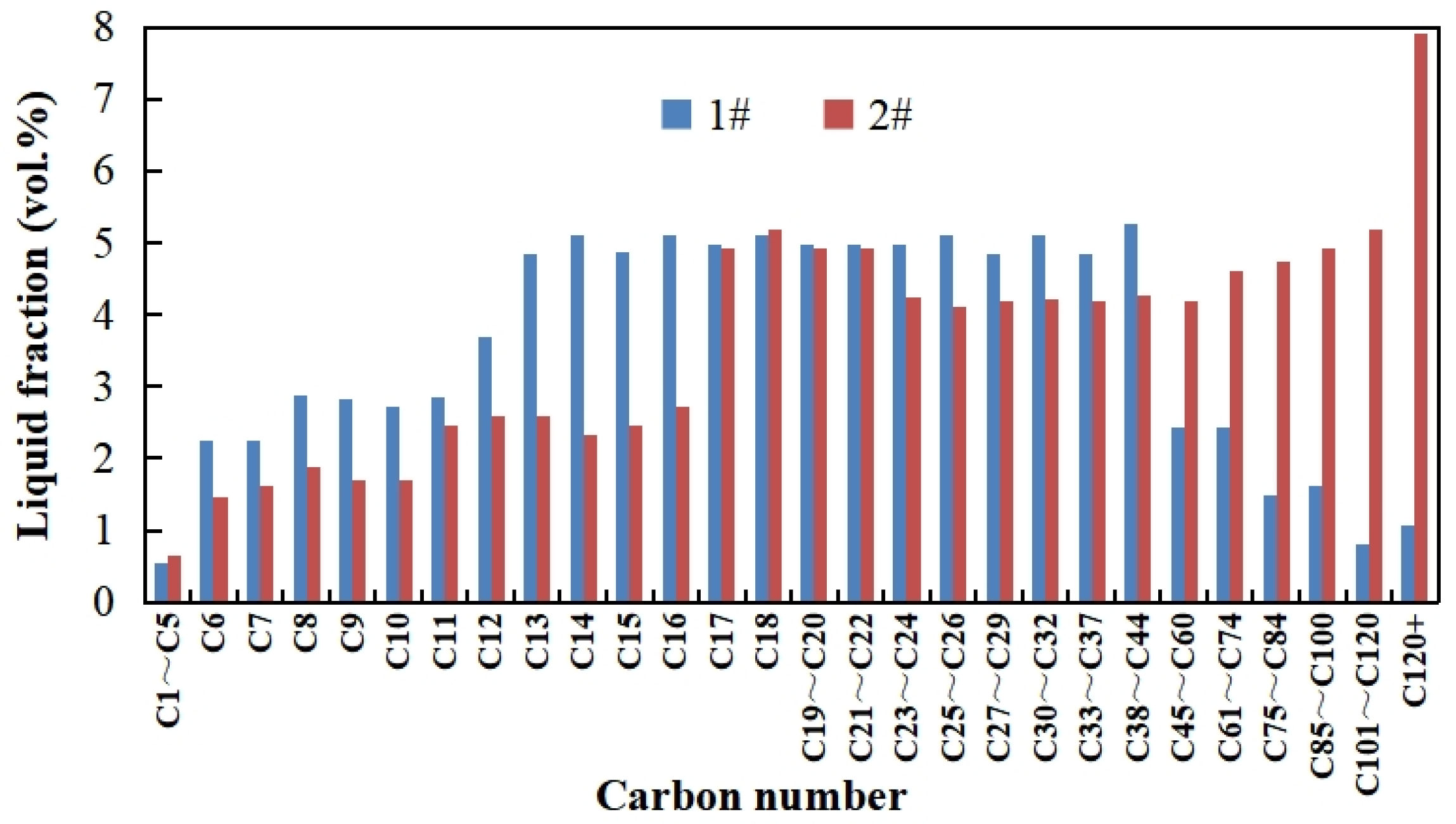
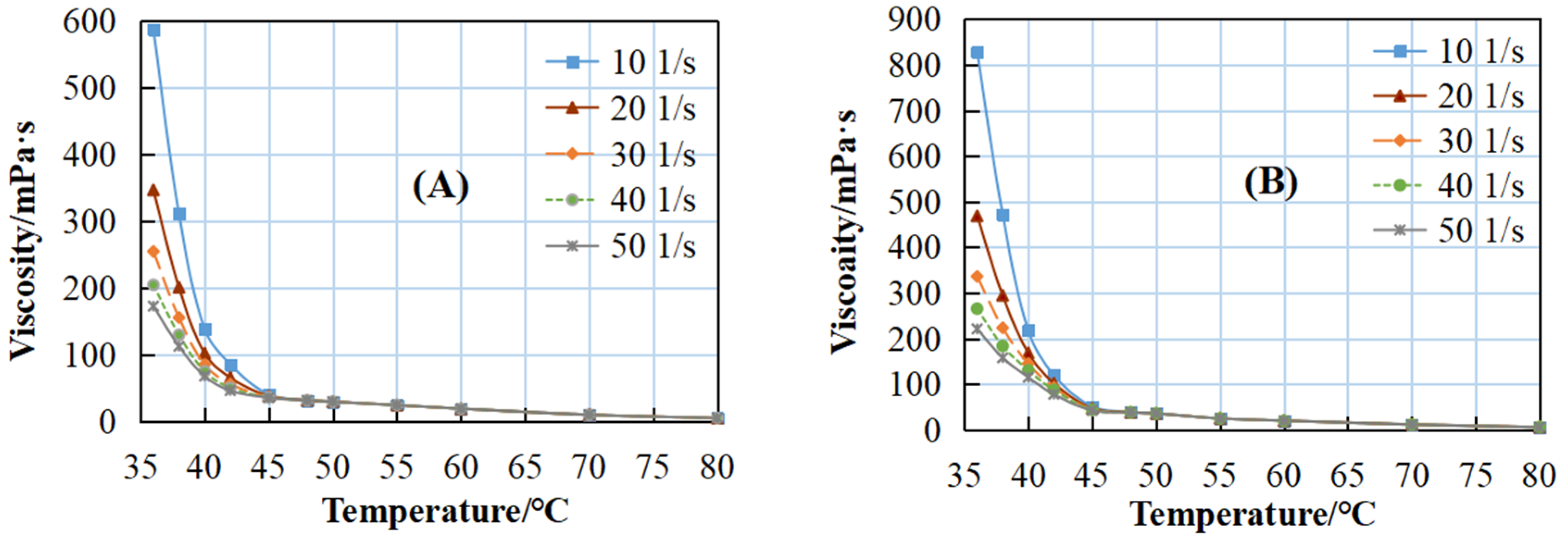
2.1. Oil Samples

Live and dead crude oil samples were collected from the old stabilization units at central gathering stations 1# and 2#. They are located in the eastern margin of the Ordos Basin, and the oil and gas resources are mainly derived from the Cretaceous sandstone layers. The light ends from the vapor of both the live and dead oil samples are presented in

Table 1. Mass fractions of the light ends in the live and dead oil samples (%).

Component	1#		2#
	Live	Dead	Live	Dead
C1	0.0306	0.0016	0.0327	0.0027
C2	0.0760	0.0140	0.1048	0.0268
C3	0.1236	0.0488	0.1820	0.0890
i-C4	0.2033	0.1198	0.2030	0.1374
n-C4	0.2692	0.1766	0.2192	0.1603
i-C5	1.2269	0.9945	0.2363	0.2028
n-C5	1.4068	1.1882	0.2390	0.2110
C6	0.5647	0.2612	0.6845	0.6295
C7	0.5011	0.2388	0.6476	0.4706
Total	4.4022	3.0435	2.5491	1.9301

, which were determined by the gas chromatography (CG) method with the Agilent 7890B instrument (Agilent, St. Clara, CA, USA). The volume fractions of hydrocarbons in the liquid phase are shown in Figure 1, obtained from the true boiling point (TBP) data from a vacuum distillation experiment. It is obvious that the 1# oil samples contain more volatile components and light hydrocarbons (C₁~C₁₆), and less long-chain hydrocarbons (C₄₅₊) than the 2# oil samples, which indicates that the components of 2# oil are heavier than 1# oil.

The basic physical properties of dead oil samples are detailed in

Table 2. Basic properties of dead oil samples.

Sample	Pour Point (°C)	Density at 20 °C (kg/m3)	WAT (°C)	Wax (mass%)	Asphaltenes (mass%)	Resins (mass%)
1#	33	862.1	50.7	22.43	2.2	10.5
2#	33	880.2	51.8	25.32	2.4	14.1

. The wax appearance temperature (WAT) and wax content were determined by differential scanning calorimetry (DSC) with the TA AUTO Q20 instrument (TA Instruments, New Castle, DE, USA). The mass fractions of asphaltenes and resins are measured by the solvent extraction method.

The relationships between the viscosity and temperature of dead oil samples, measured with a rotational rheometer from Anton Paar Rheolab QC (Anton Paar, Graz, Austria), are listed in

Table 3. The viscosity vs. temperature relationships of the dead oil samples.

Sample	Temperature (°C)	Consistency Coefficient K (mPa·sn)	Flow Behavior Index n	Viscosity (mPa·s)
				10 s−1	20 s−1	50 s−1
1#	36	537.12	0.6003	213.98	162.20	112.46
	38	155.40	0.7798	93.59	80.34	65.66
	41	50.36	0.9866	48.83	48.38	47.79
	45	42.03	1	42.03
	50	34.90	1	34.90
	60	22.05	1	22.05
	70	10.20	1	10.20
	80	8.53	1	8.53
2#	36	729.06	0.5701	270.93	201.12	135.64
	38	282.50	0.6595	128.98	101.86	74.56
	40	106.07	0.8212	70.27	62.08	52.70
	42	49.88	0.9807	47.71	47.08	46.25
	50	40.61	1	40.61
	60	25.90	1	25.90
	70	11.38	1	11.38
	80	8.86	1	8.86

. The viscosity increases with the decrease in temperature, mainly because of the precipitation of wax components below the WAT. When the temperatures are below 41 °C for the 1# oil and 42 °C for the 2# oil, the samples become shear thinning fluids, because higher shear rates cause greater disruption to the structure formed by wax crystals. Their viscosity declines with the increasing shear rate, following the power–law relationship in Equation (1).

$$\eta =K·{\gamma }^{n-1}$$

(1)

where η is the dynamic viscosity of the fluid, mPa·s; K is the consistency coefficient, mPa·sⁿ; γ refers to the shear rate, s⁻¹; and n is the flow behavior index.

For shear-thinning fluids, n < 1. In Table 3, n becomes smaller at lower temperatures, which indicates that the effect of shear rate on viscosity is stronger. It is because more precipitated wax crystals form a stronger three-dimensional network structure, which is more sensitive to the changes in shear rate. In addition, the viscosity of the 2# oil sample is larger than that of the 1# oil sample under the same temperature, due to the higher wax content and heavier hydrocarbons.

If part-produced water is retained in the three-phase separator for transporting water-containing crude oil, the water phase will exist as emulsified droplets. The water fractions of the 1# emulsion and 2# emulsion collected from the oilfield were about 24% and 26%. In order to acquire the viscosity of the emulsions with various water fractions, laboratory-prepared water-in-oil emulsions were analyzed with an inverse technique, which can be referred to in the previous study [14]. The viscosity–temperature relationship of the emulsion samples with a water fraction of 20% is shown in Figure 2. Compared with crude oil, the shear-thinning characteristics show up at higher temperatures (both emulsion samples at 45 °C). Furthermore, the viscosity of the emulsions is larger and more sensitive to shear rate than oil at the same temperature. On one hand, some wax crystals adsorb on the oil–water interface, enhancing the connection among wax crystals and the strength of the wax network. On the other hand, the water droplets warped in the wax network are easy to deform, leading to the low shear resistance of the emulsion systems. In addition, influenced by the difference in the viscosity of the oil phases, the 2# emulsion is more viscous than the 1# emulsion, especially in the non-Newtonian region.

2.2. Calculation and Test Methods of Phase Equilibrium Characteristics

2.2.1. Simplified Calculation Method of Equilibrium Constant

The bubble point (BP) lines of live oils were calculated using the simplified equilibrium constant method [42,43]. Several assumptions were made in the process: non-alkanes in the crude oil were treated as the corresponding alkanes with the same carbon number, and hydrocarbons heavier than C₆ were combined into a single pseudo-component represented as C₆+. Iterative calculations were conducted when the live crude multi-component system at the BP conformed to Equations (2) and (3).

$${\displaystyle \sum K_i{x}_i}-1=0$$

(2)

$$x_i=z_i$$

(3)

here, $x_i$ and $z_i$ refer to the mole fractions of component i in the liquid phase and system, respectively, and $z_i$ can be easily calculated using the data provided in Table 1. $K_i$ is the equilibrium constant of component i, which can be obtained from the hydrocarbon p-t-K nomogram. The value of $K_{{\mathrm{C}}_6+}$ is calculated to be 0.11 $K_{{\mathrm{C}}_6}$.

2.2.2. Aspen HYSYS Simulation of Phase Equilibrium Characteristics

In Aspen HYSYS V12 software, the compositional fluid model was employed to define the live crude oil, with the light ends data input as shown in Table 1. Based on the TBP data from the vacuum distillation experiment, the pseudo-multiple system method was used to segment the heavy hydrocarbons into narrow fractions, which were then defined as the virtual components listed in

Table 4. Properties of hypothetical components.

NO.	1#			2#
	Average Boiling Point (°C)	Volume Fraction (%)	Relative Density at 15.6 °C	Average Boiling Point (°C)	Volume Fraction (%)	Relative Density at 15.6 °C
1	46.4	2.48	0.7130	65.3	1.55	0.7268
2	72.6	2.56	0.7320	97.0	1.89	0.7488
3	101.2	2.89	0.7516	116.6	1.71	0.7618
4	122.6	2.83	0.7657	137.7	1.69	0.7753
5	138.1	2.73	0.7755	163.3	2.46	0.7911
6	151.2	2.86	0.7837	193.5	2.59	0.8089
7	160.7	3.69	0.7895	219.1	2.59	0.8234
8	172.6	4.85	0.7967	238.7	2.32	0.8342
9	192.9	5.11	0.8085	256.8	2.46	0.8439
10	217.9	4.86	0.8227	277.9	2.73	0.8550
11	242.9	5.11	0.8365	297.5	4.91	0.8650
12	266.7	4.98	0.8491	315.6	5.18	0.8741
13	290.5	5.11	0.8615	333.7	4.91	0.8829
14	314.3	4.98	0.8734	353.3	4.91	0.8923
15	339.3	4.98	0.8856	375.9	4.91	0.9029
16	366.7	4.98	0.8986	403.0	5.18	0.9153
17	394.0	5.11	0.9113	431.7	4.91	0.9281
18	421.4	4.85	0.9236	461.8	5.18	0.9411
19	450.0	5.11	0.9361	505.5	4.77	0.9594
20	484.5	4.85	0.9507	553.8	5.18	0.9789
21	528.6	5.25	0.9688	599.0	4.91	0.9964
22	582.1	2.42	0.9899	659.3	5.05	1.0188
23	635.7	2.42	1.0102	718.1	4.91	1.0398
24	675.0	1.48	1.0245	767.8	5.18	1.0569
25	708.3	1.62	1.0364	819.1	2.46	1.0740
26	736.9	0.81	1.0464	880.9	2.46	1.0939
27	753.6	1.08	1.0521	2.48	1.50	1.1131
28	-	-	-	2.56	1.50	1.1245

.

After defining the fluid, the Peng–Robinson Cubic Equation of State (PR EoS), as described in Equation (4) [44], was used in the simulation environment to calculate the phase characteristics, obtaining the p-T phase diagram of the live and dead crude oils. For gas–liquid equilibrium calculations, the PR EoS and the Soave–Redlich–Kwong EoS (SRK EoS) [45] are among the most widely used. The choice of the PR EoS in Aspen HYSYS addressed some limitations of the SRK EoS, particularly by improving the liquid density predictions and adjusting the K_i values (except for methane).

$$\left\{\begin{array}{l}p={\displaystyle \frac{RT}{v-b}}-{\displaystyle \frac{a\left(T\right)}{v\left(v+b\right)+b\left(v-b\right)}}\\ a\left(T\right)=a_{\mathrm{c}}·\alpha \left(T\right)=0.45724{\displaystyle \frac{{\left({RT}_{\mathrm{c}}\right)}^2}{p_{\mathrm{c}}}}·\alpha \left(T\right)\\ b=0.07780{\displaystyle \frac{{RT}_{\mathrm{c}}}{p_{\mathrm{c}}}}\\ \alpha (T)={\left[1+k\left(1-{T_{\mathrm{r}}}^{0.5}\right)\right]}^2\\ \\ k=0.37464+1.54226\omega -0.26992{\omega }^2\end{array}\right.$$

(4)

where T_c and p_c refer to the critical temperature and critical pressure, respectively; T_r is the reduced temperature; $\alpha (T)$ is the function of T_r; $\omega$ is the acentric factor; and a, b, and k are coefficients.

Considering the future application of oil–water mixed transportation, a gas–liquid–liquid three-phase flash calculation for live crude oils was conducted using Aspen HYSYS software. The effects of water fraction on the BP line and gasification rate were analyzed under pipeline operating conditions.

2.2.3. Bubble Point Pressure Test

An HBPVT300/70 oil–gas phase state characteristics analyzer from Yangzhou Huabao Petroleum Instrument (Yangzhou, China) was used for the constant mass expansion test. Live crude oil was introduced into the PVT cell via an injection pump system under high pressure, and the cell temperature was set to the test temperature. The vessel pressure was then gradually reduced under isothermal conditions. During this process, the oil sample was observed using high-pressure microscopy. The pressure at which gas began to form was identified as the BP pressure at the test temperature.

2.3. Simulation of the Flowing State of Water-Containing Live Crude Oil in Pipelines

After the optimization project is completed, the export pipelines from the central gathering stations will transport water-containing live crude oil to the LT Oil Depot. The operating parameters for transportation will need to be optimized. Temperature and pressure changes along the 1# and 2# export pipelines under various transportation conditions were simulated using Pipephase 9.6 software.

2.3.1. Properties of Water-Containing Live Crude Oil

The fluid type “Compositional/Blackoil” was used to define the water-containing live crude oil. It is more flexible in fluid simulations, especially when the fluid exhibits black oil characteristics in the pipeline transportation simulation, while more detailed compositional analysis is required in the phase behaviors calculation. This combined model effectively addresses the needs of both scenarios. It offers a balance between accuracy and computational efficiency, ensuring the flexibility and efficiency of the simulation. Light ends and TBP cuts were entered as shown in Table 1 and Table 4. The PR EoS was utilized to calculate the phase characteristics within the thermodynamic system. “Petroleum Correlations” were selected for calculating the parameters in the transport property system. In “Oil/Water Mixing”, the “Adjust Mixing Data” option was used to input the viscosity data for water-in-oil emulsions based on the experimental data.

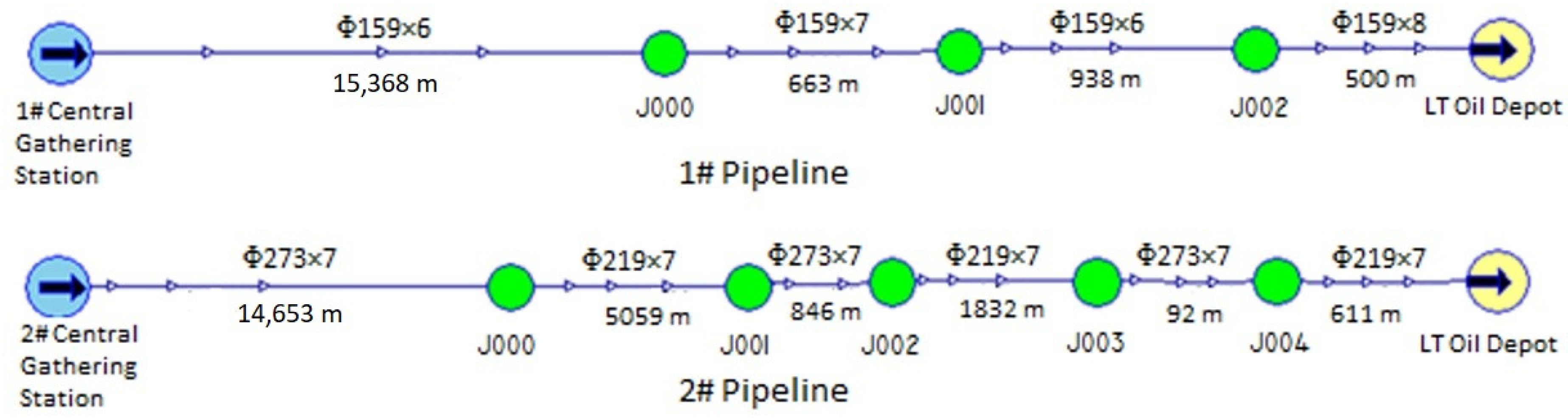
2.3.2. Pipeline Description

In the “Network Model” simulation mode, the export oil pipeline geometry models, as shown in Figure 3, were created based on the basic parameters provided in

Table 5. Basic parameters of export oil pipelines.

Pipeline	1#	2#
Size (mm)	Φ159 × 6/7/8	Φ219 × 7/Φ273 × 7
Total distance (km)	17.46	23.09
Overall coefficient of heat transfer (W/(m2·°C))	1.35	0.90
Designed capacity (×105 t/a)	4.50	9.00
Actual output (×105 t/a)	1.37	2.45
Minimum allowable output (×105 t/a)	1.93	2.59
Elevation (m)	0
Buried depth (m)	1.5
Roughness (mm)	0.20
Minimum/maximum soil temperature (°C)	8/20
Maximum allowable pressure (MPa)	1.20
Maximum allowable temperature (°C)	80
Minimum outlet temperature (°C)	36

. To prevent internal corrosion and the perforation of the pipe wall, some sections of the old pipes were replaced, resulting in variations in diameter and wall thickness within the same pipeline.

In Table 5, according to the experiment, the roughness of the inner wall of the steel pipe under normal operating conditions was 0.20 mm. Due to the corrosion thinning of the pipe wall, the maximum allowable pressure was reduced to 1.20 MPa, compared to 1.60 MPa for a new pipeline. According to the Technological Standard for Buried Steel Pipeline Asphalt Anticorrosive Coating of the Petroleum and Natural Gas Industry [46], the temperature of the pipeline transporting medium should not exceed 80 °C; thus, the maximum outlet temperature was set at 80 °C. Additionally, following the Code for Operation of Oil Pipelines of the Petroleum and Natural Gas Industry [47], which states that the minimum pipeline outlet temperature should be at least 3 °C above the pour point to prevent oil gelation, the minimum outlet temperature was set at 36 °C.

2.3.3. Simulation Under Different Pipeline Transportation Conditions

The impact of various operating parameters on the flow behavior of water-containing live oil in export pipelines was analyzed. The simulation calculated temperature and pressure variations along the pipelines based on specific outlet operating parameters. The design of the simulation variables is detailed in

Table 6. Design of variables in the simulation of pipeline transportation conditions with Pipephase.

Soil Temperature (°C)	Oil Output (m3/h)		Outlet Pressure (MPa)	Outlet Temperature (°C)	Water Fraction (vol%)
	1#	2#
8, 12, 16, 20	18	27	0.20	38	15
12	16, 17, 18, 19	23, 25, 27, 29	0.20	38	15
12	18	27	0.15, 0.20, 0.30, 0.40	38	15
12	18	27	0.20	36, 37, 38, 39	15
12	18	27	0.20	38	10, 15, 20, 25

.

In the “Thermal Calculation”, the U-value method was chosen for the heat transfer analysis. The total heat transfer coefficients were determined using historical data from actual pipeline operations over the past year. For this low-flow-rate pipeline, the flow rate was low, and the temperature drop was relatively large. Additionally, its length was short, and its diameter was relatively small compared to other long-distance oil transportation pipelines. In such pipelines, the effect of frictional heat is typically considered negligible, and temperature changes are usually calculated using the Sukhov correlation [48], as shown in Equation (5). In this study, the Sukhov correlation was used in the reverse calculation of the total heat transfer coefficients [14]. The average data of these calculated results were used as the final values, which are presented in Table 5.

$$T_{\mathrm{L}}=T_0+\left(T_{\mathrm{R}}-T_0\right)\exp \left(-{\displaystyle \frac{K\pi D}{cG}}L\right)$$

(5)

where T_L is the fluid temperature at a certain distance from the pipeline inlet, °C; T_R is the fluid temperature at the pipeline inlet, °C; T₀ is the soil temperature at the average buried depth of pipeline, °C; K is the overall heat transfer coefficient of pipeline, W/(°C·m²); $D$ refers to the pipeline diameter, m; c is the specific heat capacity of crude oil, J/(kg·°C); G is the mass flowrate, kg/s; and L is the pipeline length, m.

The pressure variations were calculated using the Beggs and Brill–Moody–Eaton method. The Beggs and Brill model [49]. was used to calculate the pipeline pressure drop. Based on the principle of energy conservation, which accounts for pressure energy, kinetic energy, potential energy, and friction loss in horizontal pipe flow, Beggs and Brill proposed the pressure drop model presented in Equation (6). The friction coefficient was obtained by the Moody method [50]. The liquid holdup was calculated according to the correlations provided by Eaton et al. [51].

$$-{\displaystyle \frac{\mathrm{d}p}{\mathrm{d}l}}={\displaystyle \frac{\left[{\rho }_l{H}_l+{\rho }_g\left(1-H_l\right)\right]g\sin \theta +\frac{\lambda Gv}{2DA}}{1-\left\{\left[{\rho }_l{H}_l+{\rho }_g\left(1-H_l\right)\right]{vv}_{sg}\right\}/p}}$$

(6)

In the formula, $p$ refers to the pipeline pressure, Pa; $l$ is the pipeline length, m; ${\rho }_l$ and ${\rho }_g$ are the densities of the liquid and gas, kg/m³; $v$ is the mean velocity of the gas–liquid mixture and the gas, m/s; $v_{sg}$ is the apparent velocity of the gas, m/s; $g$ is the gravity acceleration, m/s²; $\theta$ is the inclination of the pipeline, °; A is the flow area, m²; $\lambda$ denotes the friction coefficient, dimensionless; and $H_l$ is the liquid holdup, dimensionless.

3. Results and Discussion

3.1. Phase Diagram of Live Crude Oil

3.1.1. p-t Phase Diagram of Live and Dead Oils

The p-t phase diagrams of the live and dead oils, simulated using Aspen HYSYS software, are shown in Figure 4. The phase states are divided into three regions by the BP line and dew point (DP) line. When the temperature and pressure of the crude oil are on the upper left side of the BP line, the crude oil is entirely in the liquid phase. When the temperature and pressure of the crude oil are on the right side of the DP line, the crude oil is entirely in the gas phase. If the temperature and pressure of the crude oil are in the middle area enclosed by the BP line and the DP line, the crude oil is in the two-phase (gas–liquid) region. The point where the BP line and the DP line connect is the critical point, where the densities of the liquid and gas are the same and cannot be distinguished. On the left side of the critical point, as the temperature of the crude oil increases, the BP pressure also rises, and a higher temperature is required for the oil to be entirely in the liquid phase. On the right side of the critical point, the DP line is more sensitive to pressure changes. At higher pressures, more light components can dissolve in the liquid crude oil. Therefore, the DP temperature of the crude oil increases as the pressure decreases.

Compared to dead oils, live oils exhibit a distinct upward shift in the BP lines due to more light ends, indicating a higher possibility of gas–liquid two-phase flow in pipelines. Furthermore, the pressures of their critical points are noticeably higher than those of the dead oils, while the DP lines remain relatively unchanged. For the 2# crude oils, the critical pressures (pressure of a critical point) are lower than those of the 1# oils, which indicates that the 2# oils are more easily liquefied at high temperatures. Also, the critical temperatures of the 2# oils are higher, which shows that higher temperatures are needed to convert the 2# oils to gas at the same pressure as 1# oils. These phenomena are attributed to the heavier components in the 2# crude oil compared with the 1# oil, as illustrated in Figure 1. However, at temperatures below approximately 150 °C, the BP pressure of the 2# live oil is higher than that of the 1# live oil due to the presence of more C₁~C₃ hydrocarbons, which are more prone to evaporate at lower temperatures.

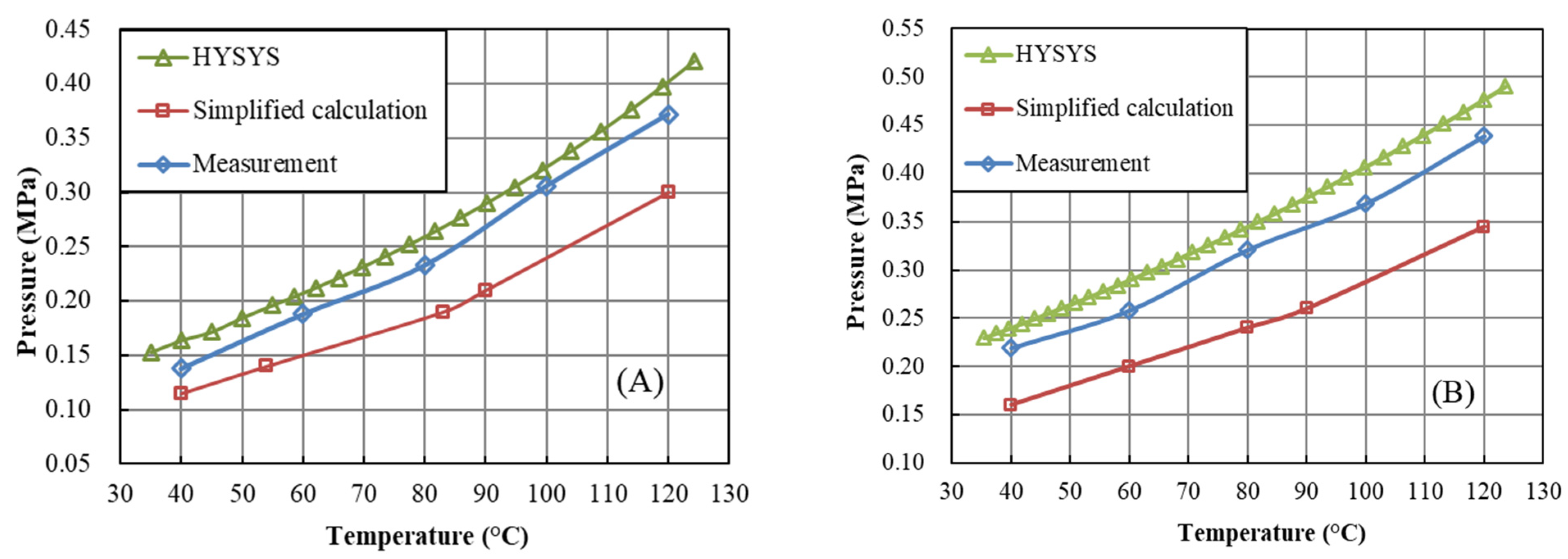
3.1.2. Comparison of Bubble Point Lines Calculated by Different Methods

The BP lines of live oils in and around the temperature range of the export pipeline obtained by different methods are shown in Figure 5.

Compared to the experimental data, the average relative errors for Aspen HYSYS and the simplified calculation method were 8.5% and −20.1%, respectively. These discrepancies stem from differences in the methods used to calculate K_i. The simplified calculation method struggled to accurately determine the quantity of each component in the gas and liquid phases due to the complexity and variability of crude oil components. It considered K_i as a function of only temperature and pressure, ignoring the effects of hydrocarbon system composition and treating all components heavier than C₆ as independent pseudo-components, leading to greater calculation errors. In addition, the experimental method used to determine bubble point pressure might have produced lower results if the precipitated gas was too minimal to observe, which could explain the difference between the experimental data and Aspen HYSYS simulation results.

3.2. Impact of Water Phase on the Gasification of Light Components

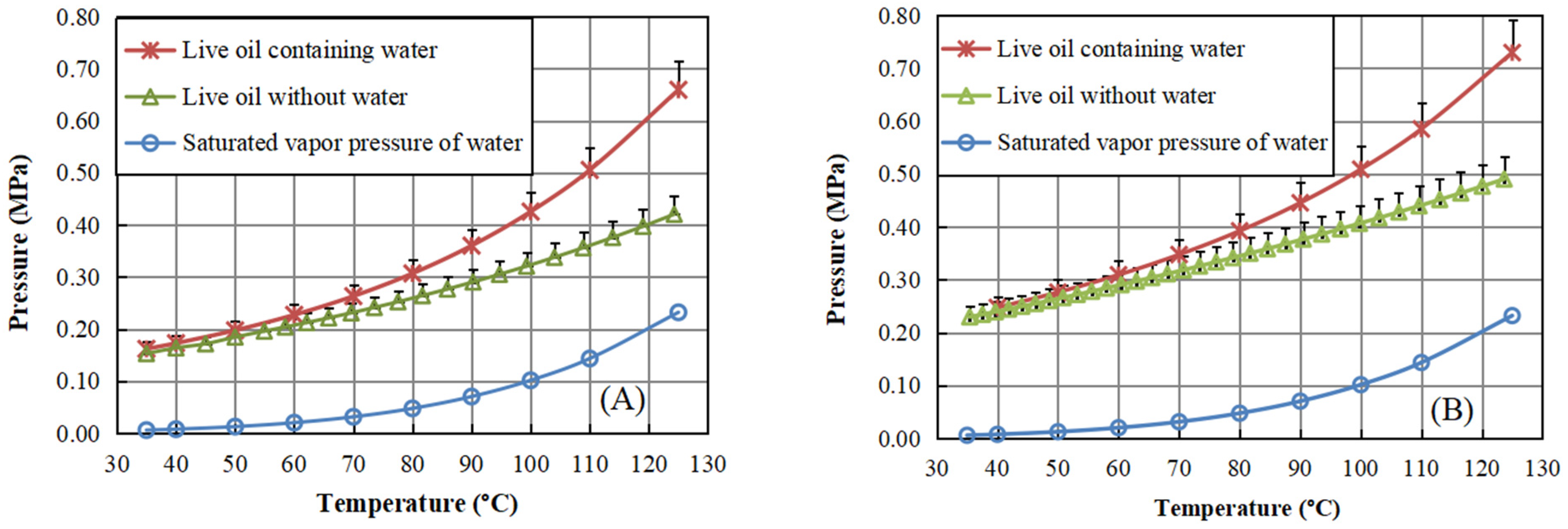
3.2.1. Bubble Point Line of Water-Containing Live Crude Oil

Figure 6 illustrates the BP lines of live oils within the temperature range typical for export pipelines, as calculated by Aspen HYSYS software. The results reveal that the BP pressure of live crude-containing water was higher than that of water-free crude oil at the same temperature. The difference in pressure corresponds to the saturated vapor pressure of the water at that temperature. Additionally, the changes in water fraction (up to 25%) have a minimal impact on the BP line within this temperature range of water-containing crude oil.

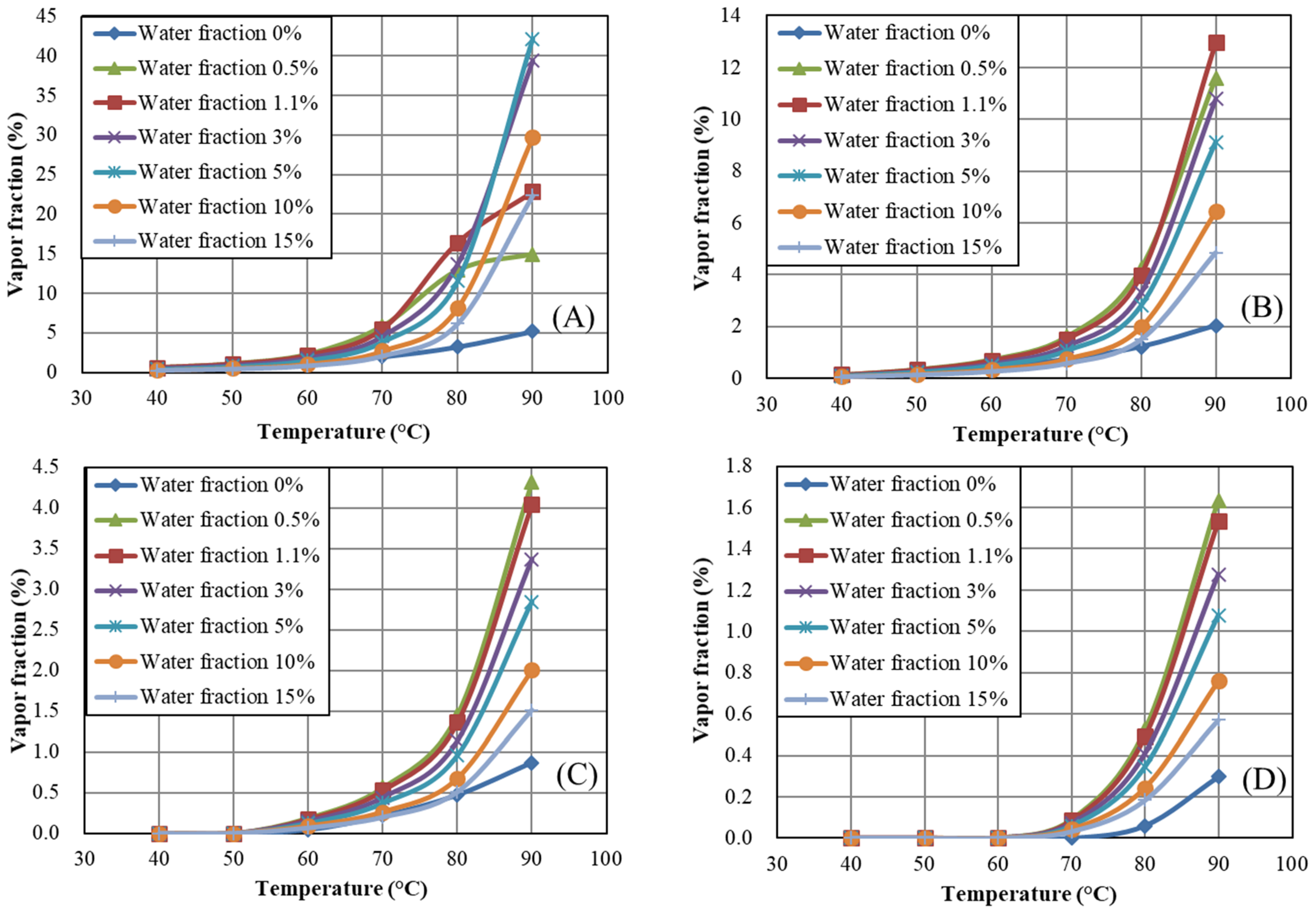
3.2.2. Influence of Water Fraction on the Vapor Fraction of Live Crude Oil

The variations in the mole vapor fraction of the 1# live oil with various water fractions under different pressure and temperature conditions are shown in Figure 7.

At the same temperature and pressure, the vapor fraction of water-containing live oil was higher than that of water-free crude oil. In the three-phase coexistence region of gas, liquid hydrocarbons, and the aqueous phase, the vapor fraction increased with temperature, with changes becoming more pronounced. Furthermore, as the pressure increased, the BP temperature gradually rose, leading to a decrease in the vapor fraction at the same temperature.

Figure 7A–D show that at lower pressures, crude oil with a higher water fraction exhibited a more significant vapor fraction, with this trend becoming more pronounced at higher temperatures. As pressure increased, a higher water fraction led to a more substantial decrease in vapor fraction. Additionally, at increasing temperatures, the vapor fraction of high-water-fraction crude oil eventually fell below that of lower-water-fraction crude oil. Specifically, at a pressure of 0.10 MPa, the vapor fraction increased with the rising water fraction from 0% to 1.1% at 80 °C and below. However, for water fractions above 1.1%, the vapor fraction decreased, with the highest vapor fraction observed at 90 °C for crude oil with a 5% water fraction. At 0.15 MPa, the highest vapor fraction shifted to crude oil, with a 1.1% water fraction at 90 °C. At 0.20 MPa, the vapor fraction of water-containing crude oil decreased with the increasing water fraction due to the reduction in the mole fraction of light components as the water fraction increased.

3.3. Analysis of the Pipeline Transportation Simulation Results

The temperature and pressure changes in the fluid along the 1# and 2# export pipelines under various transportation conditions were obtained using Pipephase. To analyze how different factors affect the fluid flow state in the pipelines, the pressure–temperature curves were compared with the fluid BP line on the p-t graph.

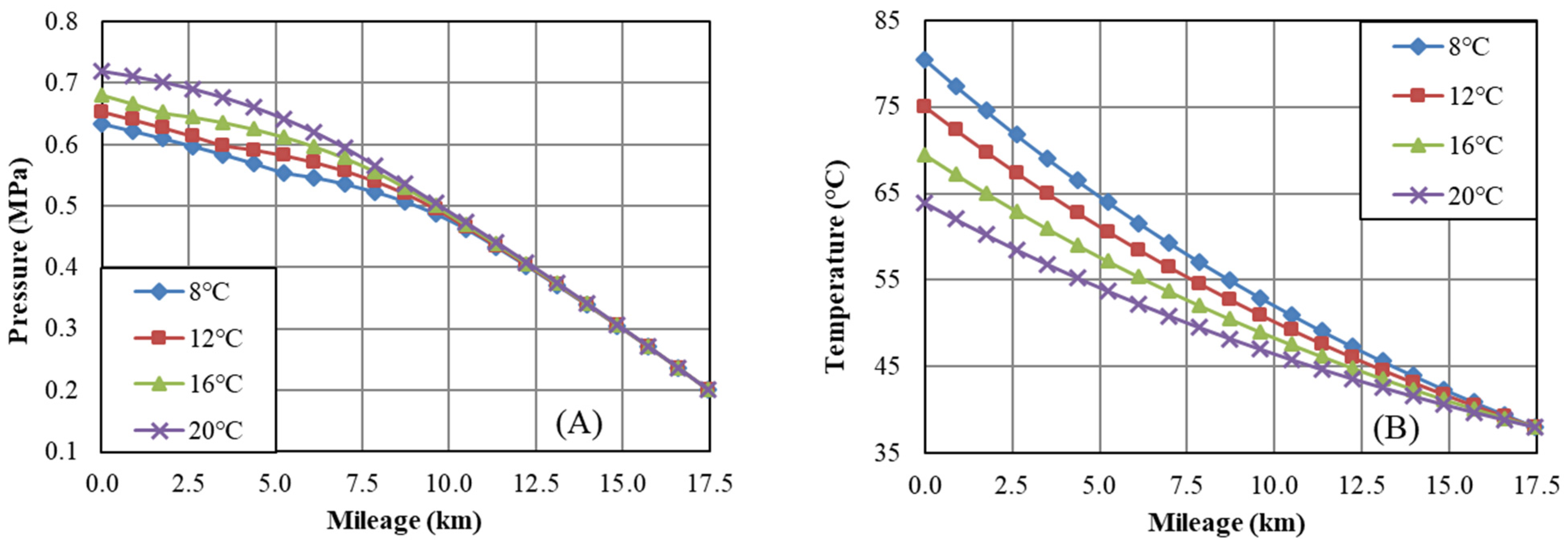
3.3.1. Impact of Soil Temperature on Fluid Flowing State

The transportation conditions of a buried pipeline are closely related to soil temperature, which varies throughout the year. Figure 8 shows the pressure and temperature changes along the 1# pipeline under different soil temperatures. It is evident that a lower soil temperature necessitates a higher inlet temperature and lower inlet pressure to achieve the specified outlet temperature and pressure. This is because a lower soil temperature increases the temperature difference between the fluid and the pipe wall, leading to greater heat dissipation during flow. As a result, there is a more pronounced temperature drop along the pipeline, requiring a higher inlet temperature to maintain an outlet temperature of 38 °C. Additionally, the higher average transportation temperature reduces the viscosity and density of the crude oil, which decreases the transportation friction and, therefore, the required export pressure at the beginning of the pipeline. These variations are consistent with previous research findings [14,52].

A comparison between the pressure–temperature curve along the pipeline and the BP line of the live oil with water under different soil temperatures is presented in Figure 9. Due to the larger diameter of the inlet pipe section in the 2# pipeline, the pressure drop of this section was more moderate, and the inlet pressure of the 2# pipeline was much smaller than the 1# pipeline. On the p-t graph, once the pressure–temperature curve falls below the BP line, it indicates that the fluid has entered the vapor–liquid region, resulting in a gas–liquid flow within the pipeline.

It is worth noting that the pressure–temperature curve for the entire 1# pipeline, as shown in Figure 9A, remained above its BP line, indicating that no vapor phase formed during transportation. In contrast, the BP line for the 2# crude oil was higher, so under the simulation conditions, the pressure and temperature at the pipeline outlet fell below this line, resulting in gas–liquid mixed flow. As the soil temperature decreased, the pipeline inlet entered the gas–liquid mixed flow region, and the length of the mixed flow section increased with further declines in soil temperature.

In winter, with low soil temperatures, the inlet temperature may need to be raised above the maximum allowable temperature of the pipeline to prevent oil gelation. This requires increasing the water fraction in the crude oil to ensure safe transportation. Under these conditions, the formation of a gas–liquid mixture is more likely in winter, typically at both the beginning and end of the pipeline. In summer, the pipeline operates at a lower average temperature and a higher inlet pressure due to the increased fluid viscosity, which necessitates careful monitoring to prevent overpressure incidents, especially in the 1# crude oil pipeline.

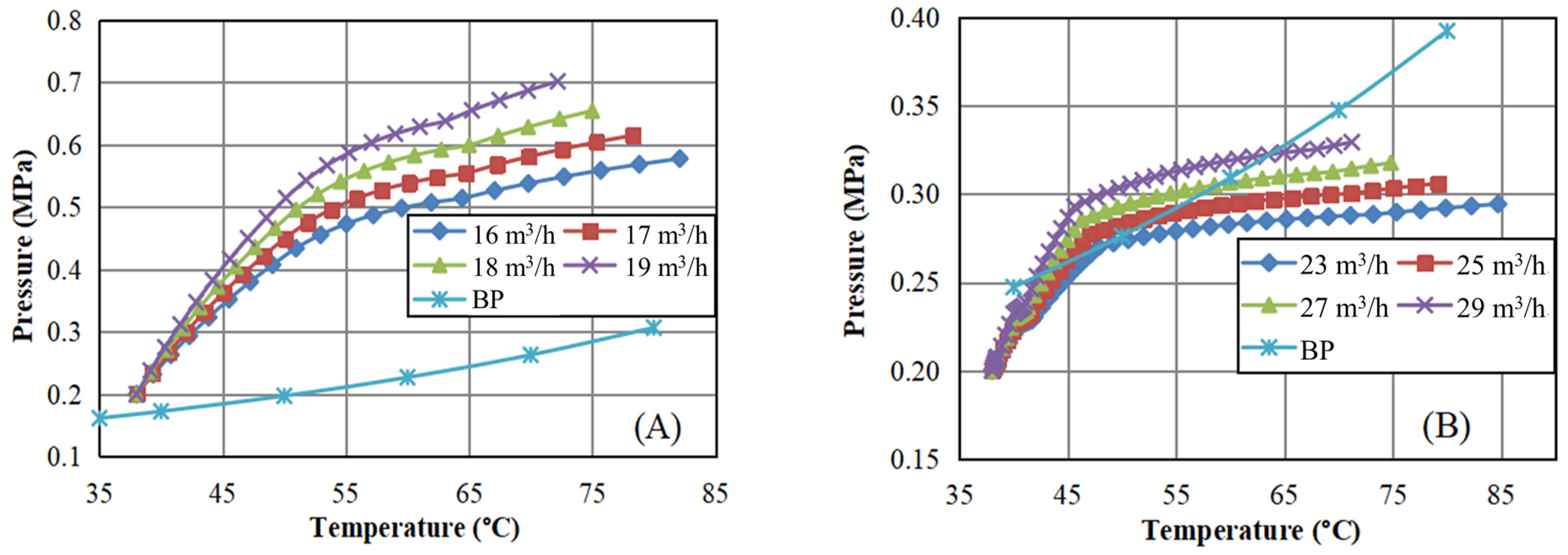
3.3.2. The Impact of Output on the Fluid Flowing State

Considering the continuous decline in the annual yield of the old oilfield, it is expected that the output from the export pipelines will continue to decrease in the future. Figure 10 illustrates a comparison between the pressure–temperature curves along the pipeline and the BP lines of the live oil with water for various levels of crude oil output.

Consequently, when other factors remained unchanged, the lower the output, the higher the inlet temperature that was needed for the pipeline, and the lower the inlet pressure. This is because a lower output induced a lower crude oil flow rate and a larger temperature reduction along the pipeline. No gas–liquid mixed transportation state was evident in the 1# crude oil pipeline. By contrast, gas evolution was apparent at the end of the 2# pipeline in these simulation conditions. With the gradual decrease in the output, the starting point of the pipeline entered the gas–liquid mixed transportation region, and had a longer mixed transportation pipeline section.

As a result, with the other factors held constant, a lower output requires a higher inlet temperature and a lower inlet pressure for the pipeline. This is due to the reduced flow rate of the crude oil and a greater temperature drop along the pipeline. No gas–liquid mixed flow was observed in the 1# crude oil pipeline. However, gas evolution was noticeable at the end of the 2# pipeline under these conditions. As the output continued to decrease, the pipeline’s starting point began to enter the gas–liquid mixed flow region, resulting in a longer mixed flow section.

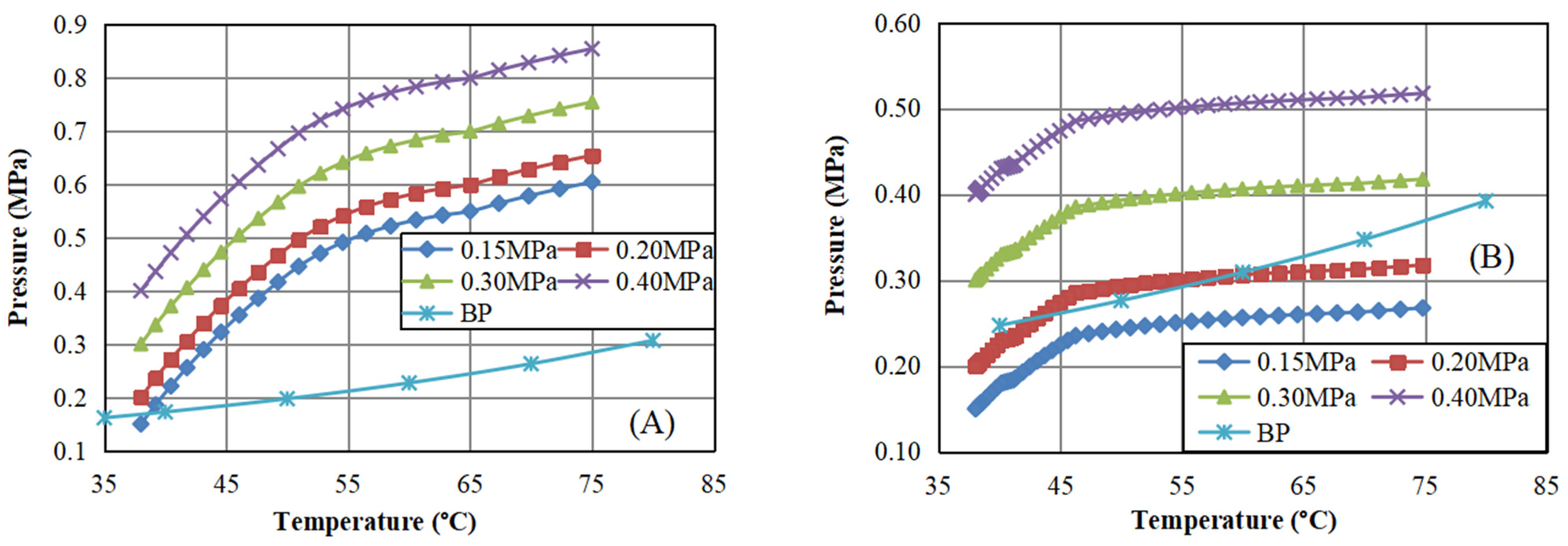
3.3.3. The Impact of Outlet Pressure on the Fluid Flowing State

Following the implementation of centralized stabilization at the downstream oil depot, it is important to consider the inlet pressure requirements of the stabilization system and reassess the outlet pressure of the export pipelines. Figure 11 compares the pressure–temperature curves along the pipeline with the BP lines of the live oil with water for various outlet pressure values.

Although changes in outlet pressure had a minimal effect on the overall profile of the pressure–temperature curves for the entire pipeline, they significantly shifted the curves up or down depending on the outlet pressure difference. This shift greatly impacted whether the pipeline enters the gas–liquid mixed transportation region. When the outlet pressure and temperature were above the BP line, the likelihood of gas–liquid mixed transportation occurring anywhere in the pipeline was low. Therefore, increasing the pipeline outlet pressure appropriately can effectively prevent gas–liquid mixed transportation. Additionally, it is important to monitor and avoid overpressure in the 1# pipeline.

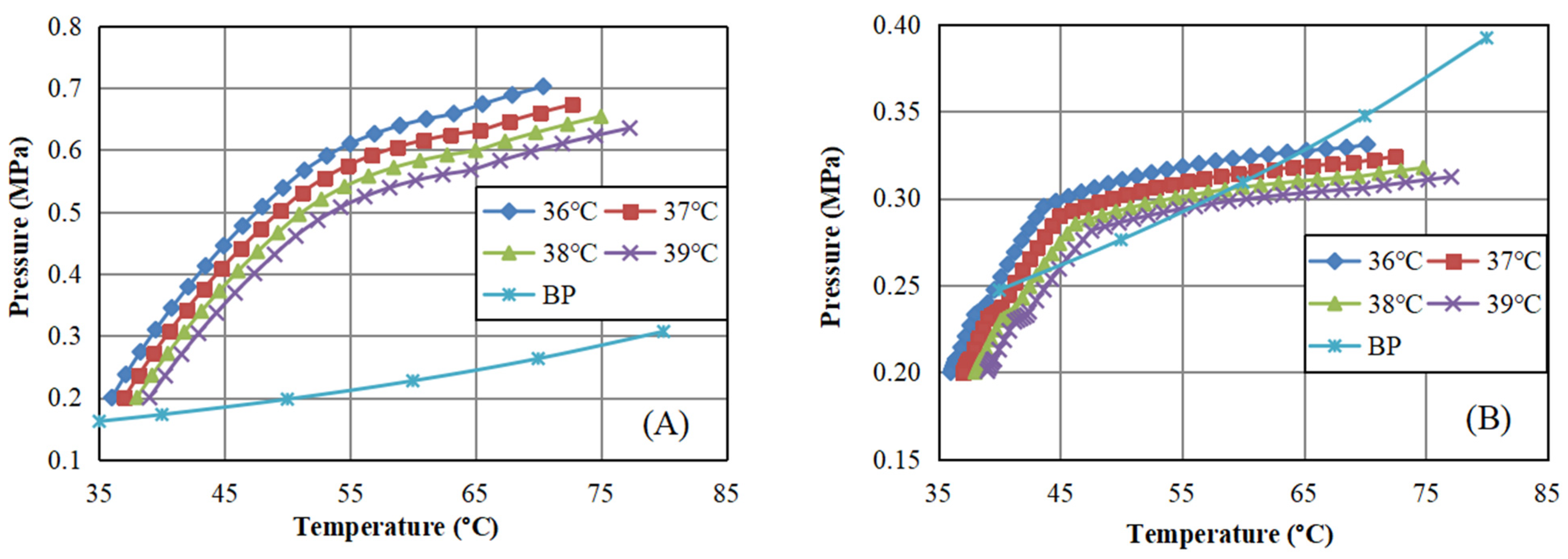
3.3.4. The Impact of Outlet Temperature on the Fluid Flowing State

The selection of outlet temperature is crucial for the safe transport of waxy crude. Figure 12 illustrates the impact of outlet temperature on the pipeline’s pressure–temperature curve.

It is evident that the changes in outlet temperature significantly affected the pressure drop in the pipeline. Higher outlet temperatures raised the overall transportation temperature along the pipeline and created a larger temperature differential between the inlet and outlet. As a result, the pipeline friction decreased, leading to a lower inlet pressure and increasing the likelihood of entering the gas–liquid mixed transportation region. Thus, while increasing the inlet temperature reduces the risk of pipeline gelation, it also raises the possibility of gas–liquid mixed transportation.

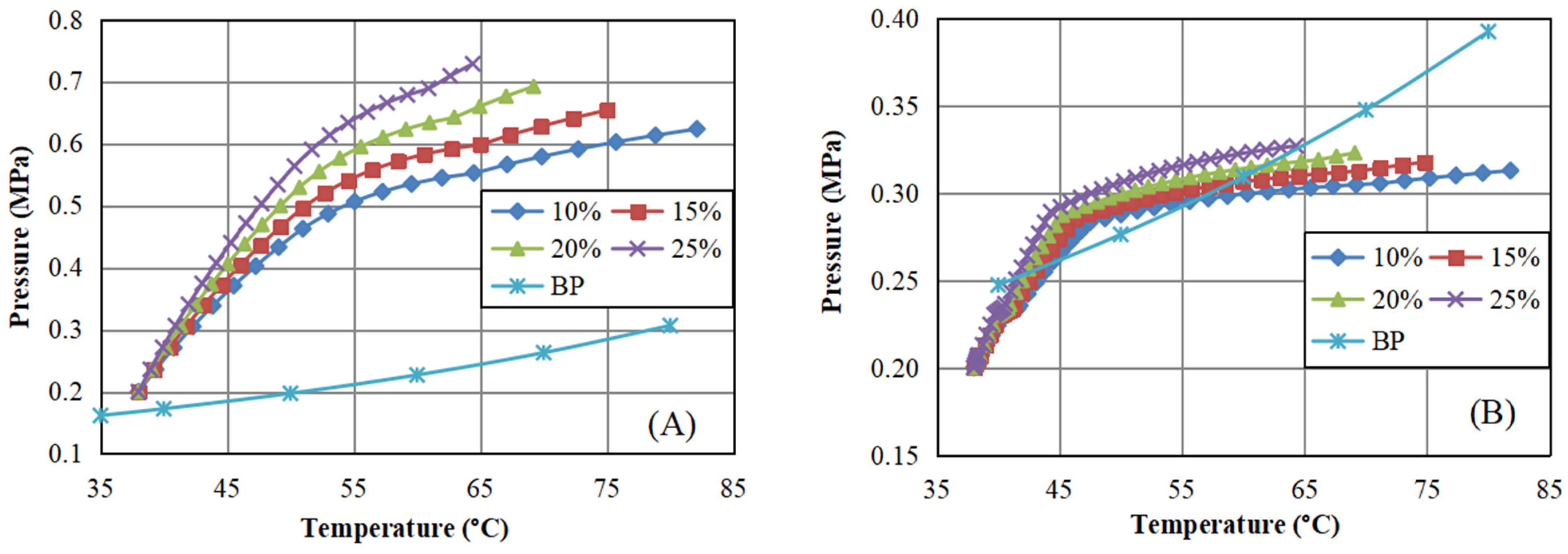
3.3.5. The Impact of Water Fraction on the Fluid Flowing State

To address the low-output issue of using oil–water mixed transportation technology, the appropriate amount of blending water must be determined based on the predicted pipeline parameters. Figure 13 displays the pipeline pressure–temperature curves and the BP lines for transporting live crude oil with different water fractions.

The results indicate that increasing the water fraction improves the overall pipeline output and reduces the required inlet temperature, which in turn raises the inlet pressure. If the oil output decreases further, raising the inlet temperature to ensure a safe outlet temperature could exceed the pipeline’s maximum allowable operating temperature and increase the risk of gas formation in the inlet section. In such cases, a higher water fraction should be used to boost the pipeline output and slow the temperature drop. Additionally, monitoring the inner pipe wall for corrosion and considering the power cost and overpressure of the 1# pipeline are important.

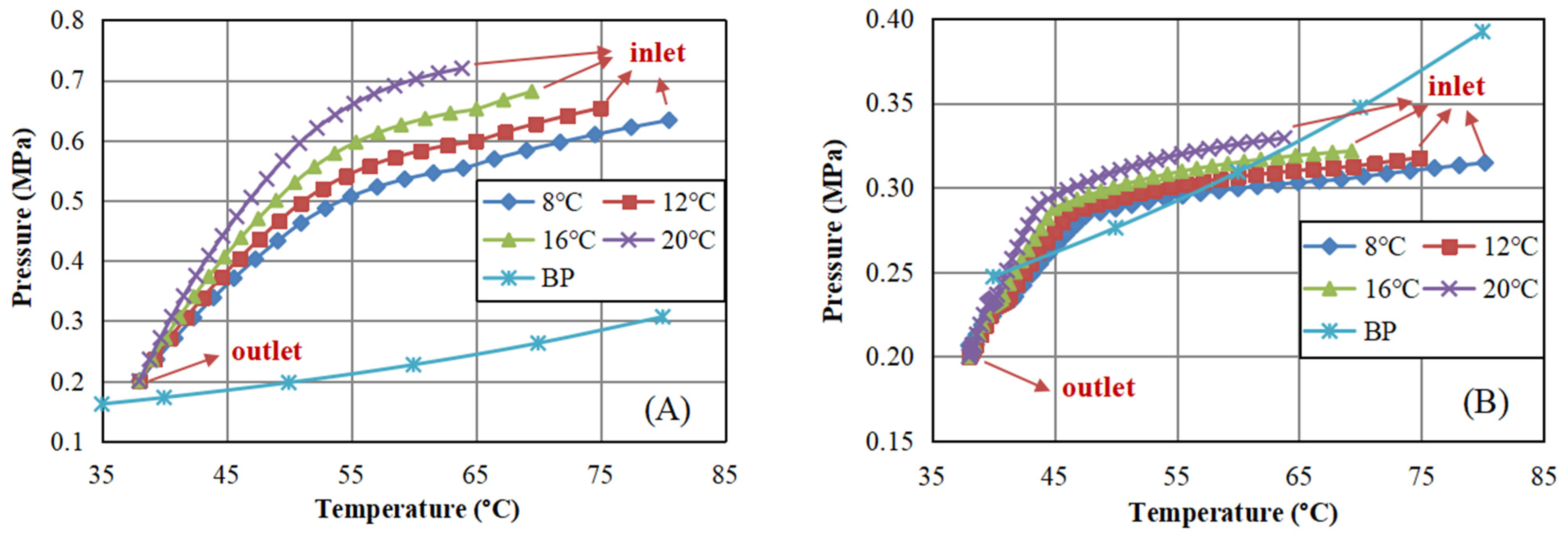
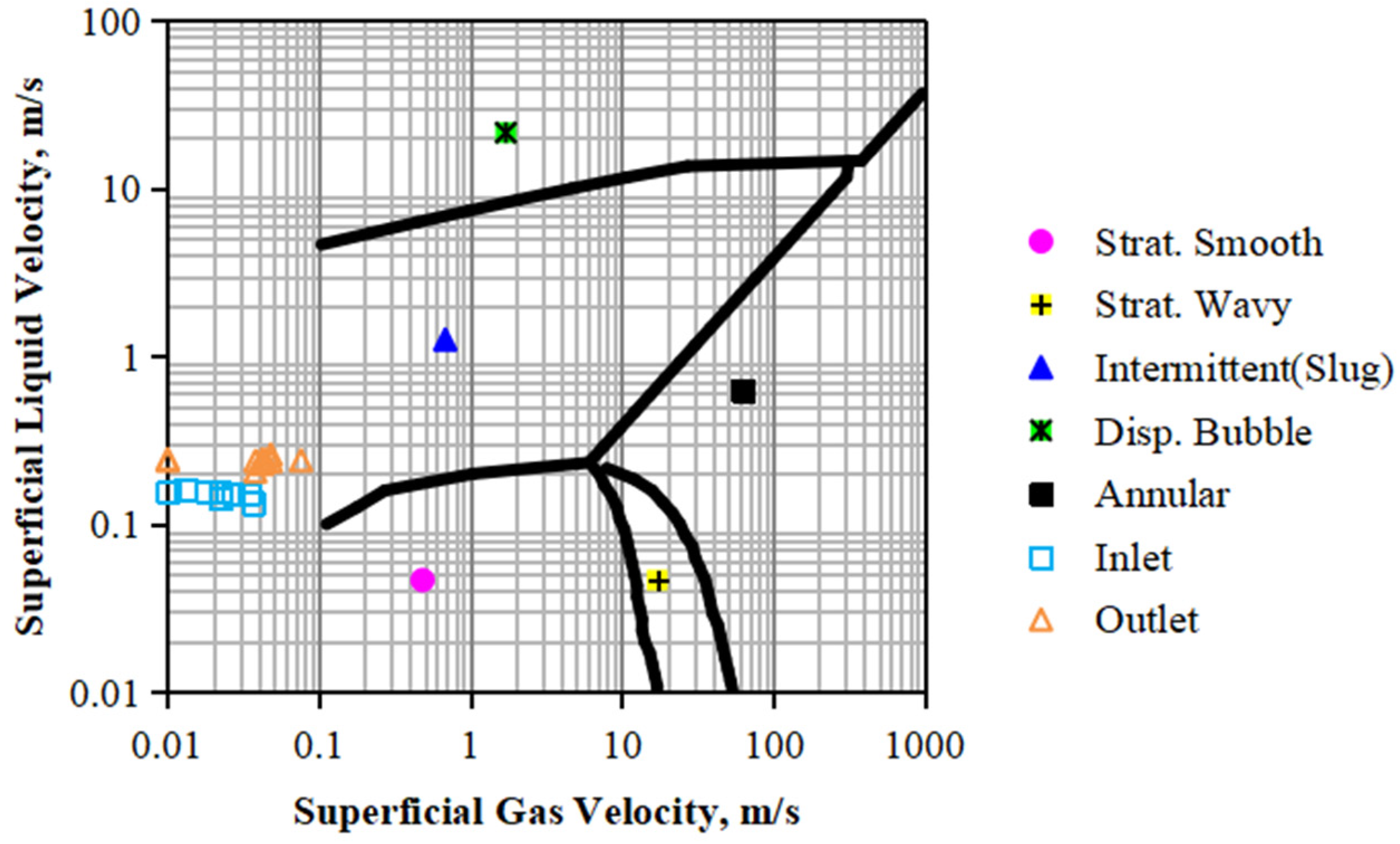
3.3.6. Characteristics and Flow Patterns of Gas–Liquid Mixed Flow in the Pipeline

Table 7. Characteristics of the gas–liquid mixed flow in the 2# pipeline.

Transporting Conditions		Pipeline Inlet				Pipeline Outlet
		Gas Flow Rate (m3/h)	Slip Liquid Holdup (%)	Lm (m)	Gas Flow Rate (m3/h)	Slip Liquid Holdup (%)	Lm (m)
Soil temperature (°C)	8	4.65	93.6	7183.4	5.75	90.2	10,775.6
	12	3.74	95.2	5131.0	5.75	90.2	10,262.5
	16	2.64	97.3	2565.5	5.75	90.2	9749.4
	20	0	100	0	5.75	90.2	9236.3
Oil output (m3/h)	23	8.02	90.2	14,366.8	5.36	90.2	11,288.7
	25	4.21	93.8	7183.4	5.55	90.2	10,775.6
	27	3.74	95.2	5131.0	5.75	90.2	10,262.5
	29	0	98.3	2052.4	5.94	90.2	9749.4
Outlet pressure (MPa)	0.15	7.02	91.0	23,093.0	9.37	88.4	23,093.0
	0.20	3.74	95.2	5131.0	5.75	90.2	10,262.5
	0.30	0	100	0	0	100	0
	0.40	0	100	0	0	100	0
Outlet temperature (°C)	36	0	99.1	1539.3	5.28	92.9	8723.2
	37	1.78	97.5	3078.6	5.46	91.7	9749.4
	38	3.74	95.2	5131.0	5.75	90.2	10,262.5
	39	4.37	93.6	6670.3	5.84	89.8	11,288.7
Water fraction (vol%)	10	5.19	93.1	6670.3	6.08	90.0	11,288.7
	15	3.74	95.2	5131.0	5.75	90.2	10,262.5
	20	2.45	97.8	2565.5	5.51	90.6	9749.4
	25	0	100	0	5.36	90.8	9236.3

Note: L_m refers to the length of the gas–liquid mixed flow section at the pipeline inlet or outlet.

summarizes the key parameters for gas–liquid mixed flow at the inlet and outlet of the 2# pipeline. The results show that light components are more prone to vaporization under the following conditions: (1) low soil temperature, (2) low oil output, (3) low outlet pressure, (4) high outlet temperature, and (5) small water fraction. Additionally, gas–liquid mixed flow predominantly occurs at the beginning and end of the pipeline, with a lower liquid holdup nearer to the endpoints.

Based on the Taitel–Dukler flow diagram in Figure 14, intermittent flow was observed at the pipeline’s inlet or outlet sections. With low liquid and gas superficial velocities, the flow pattern was classified as bubble flow, with no severe slug flow occurring in these simulations.

3.4. Optimization of Station Process and Pipeline Operation

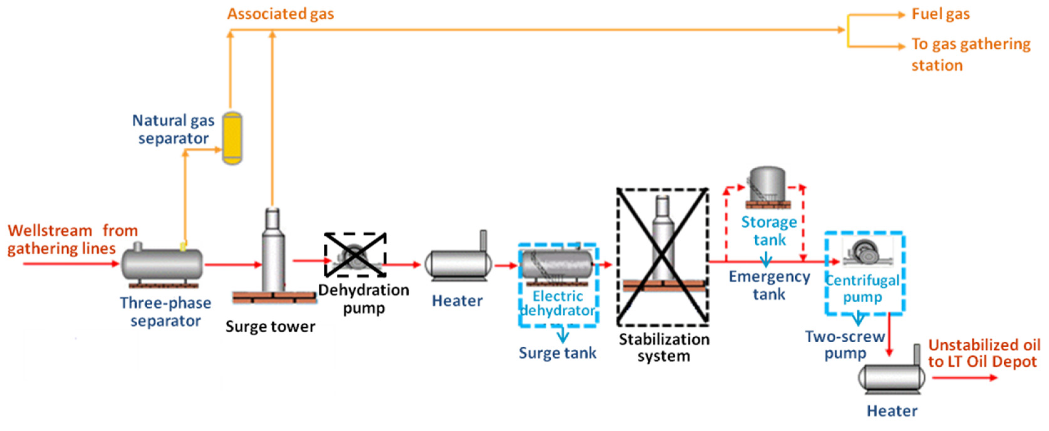
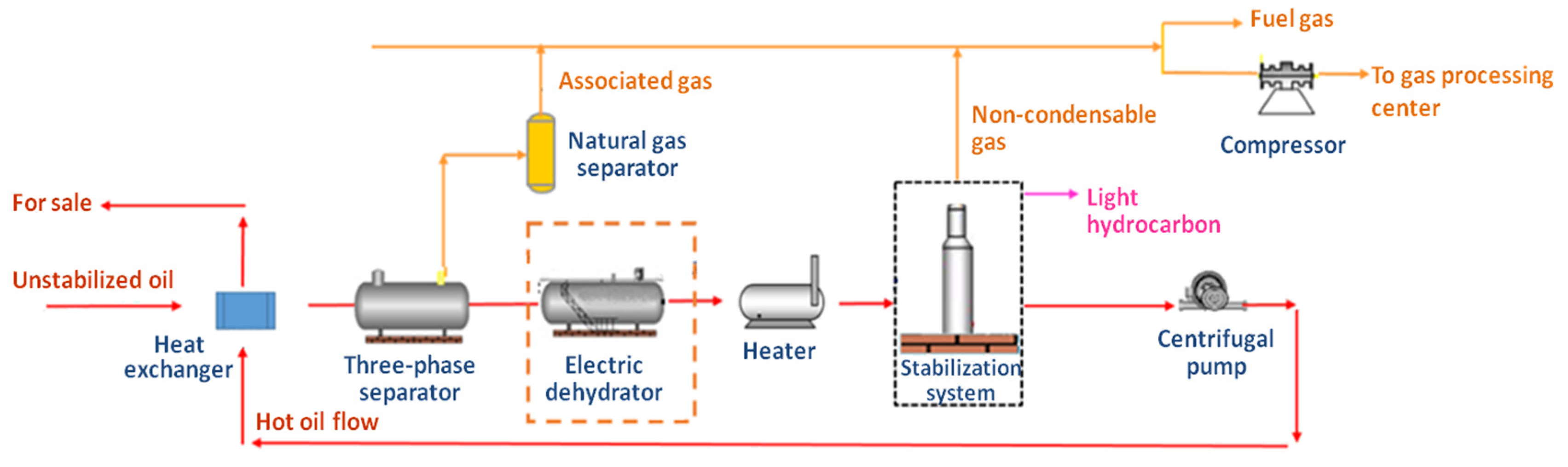
3.4.1. Optimization of the Process in the Central Gathering Station

Several optimization suggestions for the central gathering stations’ oil–water mixed-flow transportation of live crude oil are proposed. The optimized diagram is illustrated in Figure 15.

To optimize the crude oil stabilization system and improve the station’s operations, the following adjustments are recommended:

(1)

Crude Oil Stabilization System:

Centralized stabilization: Dismantle the crude oil stabilization systems at the six stations and build a new crude oil stabilization unit at the LT oil depot downstream of the pipelines to centrally process the live oil from the six pipelines. According to the corresponding calculations, after the optimization project, the total fuel gas consumption in the stabilization unit will be 1.28 × 10⁶ m³/a, decreasing by 63.9%. The total electricity consumption for one year will be 1.87 × 10⁶ kW/h, decreasing by 40.6%. In addition, the comprehensive energy consumption of the oil will decrease from 4.13 kgce/t to 1.91 kgce/t.

(2)

Pipe Network Adjustment:

Reconfigure network: Modify the pipe network within the station to align with the new operational requirements.

(3)

Dewatering System:

Stop dewatering pump: As the transportation process no longer requires the removal of emulsified water, discontinue the use of the dewatering pump.

Transform electric dehydrator: Convert the current electric dehydrator into a closed surge tank to manage the live crude oil more effectively.

(4)

Tank Adjustments:

Adjust tank storage: Given that live crude oil contains many light components, it should not be stored in an unsealed tank. Modify the original purified tank to serve as an accident tank instead.

(5)

Pump Replacement:

Upgrade pump: Replace the existing centrifugal export pump with a twin-screw oil–gas mixed pump to prevent cavitation issues caused by the dissolved gas in the live crude oil. This reduces long-term maintenance costs and the need for frequent repairs, leading to overall savings. Twin-screw pumps are often more efficient in handling oil–gas mixtures, ensuring smoother operations and reducing energy consumption compared to traditional pumps. This can lead to lower operating costs over time. Furthermore, while there is an upfront cost for replacing the pumps, the long-term benefits in terms of the reduced downtime, lower maintenance, and improved reliability can outweigh the initial investment. This contributes to a positive return on investment (ROI) in the long run. Twin-screw pumps are more suited for handling low-flow conditions, which can improve the overall performance of the system, especially in situations where the throughput might fluctuate or when precise control of the flow is needed. This adaptability can optimize the use of resources and further enhance cost-effectiveness.

According to the previous analysis, light components are readily extracted at lower pipeline pressures. To meet operational parameter requirements and prevent the gasification of these components, the inlet pressure of the live crude oil pipeline needs to be increased to 0.30–0.40 MPa. This higher pressure ensures the effective stabilization and control of the light components.

(6)

Flow Measurement:

Install multiphase flowmeter: Replace the current liquid volume flowmeter with an oil–gas–water multiphase mass flowmeter to ensure the accurate control and measurement of the gas and water fractions in the water-containing live crude oil. While calibration is essential for accurate measurement, multiphase flowmeters are often calibrated based on well-established standards and procedures. These can include periodic calibration using known flow conditions or reference systems to ensure measurement accuracy. Additionally, some flowmeters are designed to perform self-calibration, which can minimize human error. Maintenance is indeed important for ensuring the continued reliability of the flowmeters. However, regular maintenance intervals and monitoring systems are typically built into the flowmeters to alert operators when recalibration or maintenance is required. This proactive approach helps to minimize downtime and ensure consistent performance. With appropriate calibration and maintenance practices, the flowmeters can provide highly reliable data even under fluctuating flow conditions.

These measures are designed to enhance operational efficiency, safety, and accuracy in handling crude oil at the central gathering station.

3.4.2. Optimization of Pipeline Operating Parameters

Figure 16 illustrates the process flow for crude oil’s centralized stabilization at the LT Oil Depot. Upon arrival, the live crude oil undergoes several treatments: first, it passes through a heat exchanger, then a three-phase separator, followed by an electric dehydrator, and finally a heating furnace, before entering the crude oil stabilization tower.

During the transportation of water-containing crude oil, the mixture can exhibit various flow patterns, including oil–water emulsions, oil–water stratified flows, or a combination of both. These flow patterns significantly affect the fluidity of the liquid. To ensure the safe and efficient transportation, it is crucial to evaluate the fluidity of the water-containing crude oil, taking into account factors such as pour point and viscosity, based on the specific oil–water mixing conditions. The required safe outlet temperature and pressure should be optimized according to these evaluations. To balance safety and cost, the outlet temperature should be kept at a level that prevents gas precipitation while avoiding excessive heating costs.

4. Conclusions

In this paper, the phase behaviors and flow conditions of water-containing live crude oil during pipeline transportation were examined based on an optimization project in an aging oilfield with a low crude yield. The findings are as follows:

The bubble point pressure and temperature, which mark the point at which gas begins to evolve from the liquid phase, are mainly influenced by the content and composition of light ends. Oils with a higher concentration of lighter hydrocarbons tend to have lower bubble points, whereas heavier oils have higher bubble points. Compared to dehydrated dead crude, the BP line of the water-containing live crude oil exhibits a notable upward shift in the pipeline transportation temperature range on the p-t phase diagram. The vapor fraction of the water-containing live crude oil is higher than that of dehydrated dead oil, increasing with temperature and decreasing with pressure.

There is a higher likelihood of gas–liquid mixed flow in the pipeline when transporting water-containing live crude oil. This mixed flow is more probable with a low soil temperature, low oil output, low outlet pressure, high outlet temperature, and minimal water fraction. The gas–liquid mixed flow predominantly occurs at the pipeline’s beginning and end, with liquid holdup decreasing closer to the endpoint. The simulations showed an intermittent flow with no severe slugging.

Several optimization recommendations are made for central gathering stations, downstream oil depots, and pipeline operations. To prevent the gasification of light hydrocarbons, the pipeline outlet pressure should be increased to 0.30–0.40 MPa, and the outlet temperature should be kept reasonably low. Implementing oil–water mixed transportation technology can address issues related to the low pipeline output. Additionally, reserving some produced water for transportation may be cost-effective, with the optimal water proportion to be determined through further studies.

As many old onshore oilfields transition to later stages of development, production security and efficiency issues due to a low crude yield are becoming more prevalent. Similar challenges may be present in other oilfields. Different oilfields may have varying gas-to-oil ratios, and the chemical composition of crude oil can vary widely across different fields. It would be necessary to perform laboratory experiments or simulation studies to predict bubble point behavior for the specific field in question. This study provides reliable methods and valuable insights for accurate predictions and recommendations, which are worthy of being adopted and referenced by each oilfield with unique characteristics to obtain a more detailed, case-by-case analysis.

By running simulations under various operating conditions, operators can simulate different flow regimes and assess the potential risks associated with each. Quantifying the likelihood of these scenarios and evaluating their potential impacts on system integrity can guide decision-making on operating parameters and maintenance schedules. With predictive analytics, operators can adjust operating conditions dynamically to avoid or mitigate problematic flow regimes before they lead to system failures or production losses. Monitoring the flow regime transitions from liquid-only to gas–liquid mixed flow could trigger actions such as adjusting the injection rates, optimizing separation equipment, or altering flow conditions.

Operators should implement the continuous monitoring of key parameters in real-time to detect early signs of gas–liquid mixed flow. In addition, operators should develop contingency plans for worst-case scenarios where gas–liquid mixed flow could lead to severe consequences such as equipment damage, production downtime, or safety hazards. This allows them to better predict, control, and mitigate the risks associated with mixed flow, ultimately optimizing production efficiency, enhancing safety, and reducing operational costs.

References

1. Xu, X.X. Study on oil-water two-phase flow in horizontal pipelines. J. Pet. Sci. Eng. 2007, 59, 43–58. [Google Scholar] [CrossRef]
2. Huang, X.; Li, S.; Zhu, N.; Chao, K.; Fan, K. Normal temperature gathering and transportation technology of high water-cut crude oil in Dongpuoil region of Zhongyuan oilfiled. Sci. Technol. Eng. 2021, 21, 6681–6689. [Google Scholar]
3. Lu, M.; Zhu, J. Study of energy optimization technical program of Zhao II oil transfer station gathering and transportation system. Adv. Mater. Res. 2013, 765–767, 295–299. [Google Scholar] [CrossRef]
4. Huang, Z.Q.; Li, X.Y.; Zheng, G.; Xue, J.Q.; Chen, Z. Energy saving measures of oil and gas gathering system in Changqing low permeable oilfield. Adv. Mater. Res. 2012, 512–515, 1137–1142. [Google Scholar] [CrossRef]
5. Li, J.; Huang, C.; Ye, F.; Qin, M.; Zhang, W. Application of computer energy optimization method in oil and gas gathering and transportation system. J. Phys. Conf. Ser. 2021, 1744, 022045. [Google Scholar] [CrossRef]
6. Yu, P.; Lei, Y.; Gao, Y.; Peng, H.; Zhao, H. Study on the operation safety and reliability of a waxy hot oil pipeline with low throughput using the probabilistic method. ACS Omega 2020, 5, 33340–33346. [Google Scholar] [CrossRef] [PubMed]
7. Xiao, R.G.; Yi, D.R.; Yao, P.F.; Zhou, J.Q. Analysis of the operation mode and instability on the low-ffowrate running of hot-oil pipeline. Adv. Mater. Res. 2012, 614–615, 550–554. [Google Scholar] [CrossRef]
8. Li, Q.; Li, Q.; Cao, H.; Wu, J.; Wang, F.; Wang, Y. The crack propagation behaviour of CO2 fracturing fluid in unconventional low permeability reservoirs: Factor analysis and mechanism revelation. Processes 2025, 13, 159. [Google Scholar] [CrossRef]
9. Li, Q.; Li, Q.; Wu, J.; Li, X.; Li, H.; Cheng, Y. Wellhead stability during development process of hydrate reservoir in the Northern South China Sea: Evolution and mechanism. Processes 2025, 13, 40. [Google Scholar] [CrossRef]
10. Li, S.; Huang, Q.; He, M.; Wang, W. Effect of water fraction on rheological properties of waxy crude oil emulsions. J. Dispers. Sci. Technol. 2014, 35, 1114–1125. [Google Scholar] [CrossRef]
11. Pal, R. Entropy production in pipeline flow of dispersions of water in oil. Entropy 2014, 16, 4648–4661. [Google Scholar] [CrossRef]
12. Sotgia, G.; Tartarini, P.; Stalio, E. Experimental analysis of flow regimes and pressure drop reduction in oil-water mixtures. Int. J. Multiph. Flow 2008, 34, 1161–1174. [Google Scholar] [CrossRef]
13. Wang, W.; Gong, J.; Angeli, P. Investigation on heavy crude-water two phase flow and related flow characteristics. Int. J. Multiph. Flow 2011, 37, 1156–1164. [Google Scholar] [CrossRef]
14. Li, S.; Fan, K.F.; Huang, Q.Y. Evaluation of stability for flowing water-in-oil emulsion in transportation pipeline. J. Pet. Sci. Eng. 2022, 216, 110769. [Google Scholar] [CrossRef]
15. Nichita, D.V.; Broseta, D.; Elhorga, P.; Montel, F. Pseudo-component delumping for multiphase equilibrium in hydrocarbon-water mixtures. Pet. Sci. Technol. 2008, 26, 2058–2077. [Google Scholar] [CrossRef]
16. Masoodiyeh, F.; Mozdianfard, M.R.; Karimi-Sabet, J. Thermodynamic modeling of PVTx properties for several water/hydrocarbon systems in near-critical and supercritical conditions. Korean J. Chem. Eng. 2013, 30, 201–212. [Google Scholar] [CrossRef]
17. Yong, W.P.; Awang, M. Vapour–liquid equilibria for hydrocarbon/water systems using thermodynamic perturbation theory. In Proceedings of the International Conference on Intergrated Petroleum Engineering and Geosciences, Kuala Lumpur, Malaysia, 19–22 May 2014. [Google Scholar]
18. Di, Y.; Zhang, Y.; Wu, Y. Phase equilibrium calculation of CO2-hydrocarbons-water system based on Gibbs free energy minimization. Acta Pet. Sin. 2015, 36, 593–599. [Google Scholar]
19. Delahaye, A.; Fournaison, L.; Marinhas, S.; Martínez, M.C. Rheological study of hydrate slurry in a dynamic loop applied to secondary refrigeration. Chem. Eng. Sci. 2008, 63, 3551–3559. [Google Scholar] [CrossRef]
20. Gong, J.; Shi, B.H.; Wang, W.; Zhao, J.K. Numerical study the flow characteristics of gas-hydrate slurry two phase stratified flow. In Proceedings of the International Conference on Multiphase Flow, Tampa, FL, USA, 30 May–4 June 2010. [Google Scholar]
21. Gong, J.; Shi, B.H.; Zhao, J.K. Natural gas hydrate shell model in gas-slurry pipeline flow. J. Nat. Gas Chem. 2010, 19, 261–263. [Google Scholar] [CrossRef]
22. Shi, B.H.; Gong, J.; Sun, C.Y.; Zhao, J.K.; Ding, Y.; Chen, G.J. An inward and outward natural gas hydrates growth shell model considering intrinsic kinetics, mass and heat transfer. Chem. Eng. J. 2011, 171, 1308–1316. [Google Scholar] [CrossRef]
23. Tang, Y.; Saha, S. An efficient method to calculate three-phase free-water flash for water−hydrocarbon systems. Ind. Eng. Chem. Res. 2002, 42, 189–197. [Google Scholar] [CrossRef]
24. Mokhatab, S. Three-phase flash calculation for hydrocarbon systems containing water. Theor. Found. Chem. Eng. 2003, 37, 291–294. [Google Scholar] [CrossRef]
25. Hinojosa-Gómez, H.; Solares-Ramírez, J.; Bazúa-Rueda, E.R. An improved algorithm for the three-fluid-phase VLLE flash calculation. AIChE J. 2015, 61, 3081–3093. [Google Scholar] [CrossRef]
26. Pires, A.P.; Mohamed, R.S.; Mansoori, G.A. An equation of state for property prediction of alcohol-hydrocarbon and water-hydrocarbon systems. J. Pet. Sci. Eng. 2001, 32, 103–114. [Google Scholar] [CrossRef]
27. Lapene, A.; Nichita, D.V.; Debenest, G.; Quintard, M. Three-phase free-water flash calculations using a new Modified Rachford–Rice equation. Fluid Phase Equilibria 2010, 297, 121–128. [Google Scholar] [CrossRef]
28. Ahmadi, M.A.; Zendehboudi, S.; James, L.A.; Elkamel, A.; Dusseault, M.; Chatzis, I.; Lohi, A. New tools to determine bubble point pressure of crude oils: Experimental and modeling study. J. Pet. Sci. Eng. 2014, 123, 207–216. [Google Scholar] [CrossRef]
29. Medeiros, M. Mutual solubilities of water and hydrocarbons from the cubic plus association equation of state: A new mixing rule for the correlation of observed minimum hydrocarbon solubilities. Fluid Phase Equilibria 2014, 368, 5–13. [Google Scholar] [CrossRef]
30. Mortezazadeh, E.; Rasaei, M.R. A robust procedure for three-phase equilibrium calculations of water-hydrocarbon systems using cubic equations of state. Fluid Phase Equilibria 2017, 450, 160–174. [Google Scholar] [CrossRef]
31. Taitel, Y.; Barnea, D.; Brill, J.P. Stratified three phase flow in pipes. Int. J. Multiph. Flow 1995, 21, 53–60. [Google Scholar] [CrossRef]
32. Hewitt, G.F. Three-phase gas–liquid–liquid flows in the steady and transient states. Nucl. Eng. Des. 2005, 235, 1303–1316. [Google Scholar] [CrossRef]
33. Ghorai, S.; Suri, V.; Nigam, K.D.P. Numerical modeling of three-phase stratified flow in pipes. Chem. Eng. Sci. 2005, 60, 6637–6648. [Google Scholar] [CrossRef]
34. Ujang, P.M.; Lawrence, C.J.; Hale, C.P.; Hewitt, G.F. Slug initiation and evolution in two-phase horizontal flow. Int. J. Multiph. Flow 2006, 32, 527–552. [Google Scholar] [CrossRef]
35. Wahaibi, T.A.; Angeli, P. Transition between stratified and non-stratified horizontal oil–water flows. Part I: Stability analysis. Chem. Eng. Sci. 2007, 62, 2915–2928. [Google Scholar] [CrossRef]
36. Wahaibi, T.A.; Smith, M.; Angeli, P. Transition between stratified and non-stratified horizontal oil–water flows. Part II: Mechanism of drop formation. Chem. Eng. Sci. 2007, 62, 2929–2940. [Google Scholar] [CrossRef]
37. Nan, Y.T.; Yuan, Y.H.; Ming, D.D.; Bo, Z.J. Energy equation derivation of the multiphase flow pipeline. J. Petrochem. Univ. 2011, 24, 73–76. [Google Scholar]
38. Odozi, U.A. Three-Phase Gas-Liquid-Liquid Slug Flow. Ph.D. Thesis, Imperial College London, London, UK, 2000. [Google Scholar]
39. Wong, W.L. Flow Development and Mixing in Three-Phase Slug Flow. Ph.D. Thesis, University of London, London, UK, 2003. [Google Scholar]
40. Xu, J.Y. A simple correlation for prediction of the liquid slug holdup in gas/non-Newtonian fluids: Horizontal to upward inclined flow. Exp. Therm. Fluid Sci. 2013, 44, 893–896. [Google Scholar] [CrossRef]
41. Abdul-Majeed, G.H.; Al-Mashat, A.M. A unified correlation for predicting slug liquid holdup in viscous two-phase flow for pipe inclination from horizontal to vertical. SN Appl. Sci. 2019, 1, 71. [Google Scholar] [CrossRef]
42. Michelsen, M.L. The isothermal flash problem. Part I. stability. Fluid Phase Equilibria 1982, 9, 1–19. [Google Scholar] [CrossRef]
43. Guo, T.M. Multicomponent Gas-Liquid Equilibrium and Distillation; Petroleum Industry Press: Beijing, China, 2002; Volume 11, pp. 161–166. [Google Scholar]
44. Peng, D.Y.; Robinson, D.B. A new two constant equation of state. Ind. Eng. Chem. Fundam. 1976, 15, 59–64. [Google Scholar] [CrossRef]
45. Soave, G. Equilibrium constants from a modified Redlich-Kwong equation of state. Chem. Eng. Sci. 1972, 27, 1197–1203. [Google Scholar] [CrossRef]
46. SY/T 0420-97; Technology standard of petroluem asphalt coating for buried steel pipeline. Petroleum Industry Press: Beijing, China, 1997.
47. SY/T 5536-2016; Specification for operation of crude oil pipeline. Petroleum Industry Press: Beijing, China, 2016.
48. AГалкин, B.M. Thermal and Hydraulic Calculations of Crude Oil and Product Oil Pipelines; Petroleum Industry Press: Beijing, China, 1986. [Google Scholar]
49. Beggs, D.H.; Brill, J.P. A study of two-phase flow in inclined pipes. J. Pet. Technol. 1973, 25, 607–617. [Google Scholar] [CrossRef]
50. Moody, L.F. Friction factors for pipe flow. Trans. ASME 1944, 66, 671–678. [Google Scholar] [CrossRef]
51. Eaton, B.F.; Knowles, C.A.; Silberberg, I.H. The prediction of flow patterns, liquid holdup and pressure losses occurring during continuous two-phase flow in horizontal pipelines. J. Pet. Technol. 1967, 19, 815–828. [Google Scholar] [CrossRef]
52. Li, S.; Huang, Q.; Fan, K.; Zhao, D.; Lv, Z. Transportation technology with pour point depressant and wax deposition in a crude oil pipeline. Pet. Sci. Technol. 2016, 34, 1240–1247. [Google Scholar] [CrossRef]
Figure 1. Liquid volume fractions of hydrocarbons obtained from TBP experiment.
Energies 18 01116 g001
Figure 2. The viscosity–temperature relationship of the water-in-oil emulsions of (A) the 1# oil and (B) the 2# oil with a water fraction of 20% measured by the rotational rheometer method.
Energies 18 01116 g002
Figure 3. Geometry models of export pipelines in Pipephase.
Energies 18 01116 g003
Figure 4. The comparison of the p-t phase state graphs of live and dead oils simulated by Aspen HYSYS.
Energies 18 01116 g004
Figure 5. The comparison of the BP lines of (A) the 1# and (B) 2# live crude oils obtained by different methods.
Energies 18 01116 g005
Figure 6. Influence of water phase on the BP lines of (A) the 1# and (B) 2# live oils.
Energies 18 01116 g006
Figure 7. Influence of water fraction on the vapor fraction of 1# live crude oil at (A) 0.10 MPa, (B) 0.15 MPa, (C) 0.20 MPa, and (D) 0.25 MPa.
Energies 18 01116 g007
Figure 8. The (A) pressure and (B) temperature changes along the 1# pipeline under different soil temperatures.
Energies 18 01116 g008
Figure 9. The p-t curves of (A) the 1# and (B) 2# pipelines and the BP lines under different soil temperatures.
Energies 18 01116 g009
Figure 10. The p-t curves of (A) the 1# and (B) 2# pipelines and the BP lines under different oil outputs.
Energies 18 01116 g010
Figure 11. The p-t curves of (A) the 1# and (B) 2# pipelines and the BP lines under different outlet pressures.
Energies 18 01116 g011
Figure 12. The p-t curves of (A) the 1# and (B) 2# pipelines and the BP lines under different outlet temperatures.
Energies 18 01116 g012
Figure 13. The p-t curves of (A) the 1# and (B) 2# pipelines and the BP lines under different water fractions.
Energies 18 01116 g013
Figure 14. Flow pattern of the simulated cases of the 2# pipeline on a Taitel–Dukler flow diagram.
Energies 18 01116 g014
Figure 15. Optimization of the oil processing and transferring flow in the central gathering station.
Energies 18 01116 g015
Figure 16. Flow diagram of the central crude oil stabilization technology at LT Oil Depot.
Energies 18 01116 g016