Energy Trading Strategies for Integrated Energy Systems Considering Uncertainty

Abstract

To improve the stable operation and promote the energy sharing of the integrated energy system (IES), a comprehensive energy trading strategy considering uncertainty is proposed. Firstly, an IES model incorporating power-to-gas (P2G) and a carbon capture system (CCS) is established to reduce carbon emissions. Secondly, this model is integrated into a four-level robust optimization to address the fluctuation of renewable energy sources in IES operations. This not only considers probability distribution scenarios of renewable energy and the uncertainty of its output, but also effectively reduces the model’s conservatism by constructing a multi-interval uncertainty set. On this basis, a Nash–Harsanyi bargaining method is used to solve the issue of benefit allocation among multiple IESs. Finally, the energy trading model is solved using a distributed algorithm that ensures an equitable distribution of benefits while protecting the privacy of each IES. The simulation results validate the effectiveness of the proposed strategy.

1. Introduction

As traditional fossil fuel resources gradually deplete and environmental pollution worsens, the global energy system faces unprecedented challenges. This makes the energy transition a vital pathway to achieving sustainable development [1]. To address the growing global demand for green energy, further rapid advancements in related technologies are necessary [2]. Against this backdrop, integrated energy systems (IESs) provide an effective approach to optimizing energy resource allocation and improving energy efficiency through the coordination of power generation, energy storage, and load management [3,4].

Currently, several scholars have investigated the optimal operation of IESs. In [5], the optimal capacity configuration of an IES was determined by considering its economic performance. In [6], an IES planning scheme was proposed to improve the utilization of renewable energy. In [7], power-to-gas (P2G) technology was adopted to reduce the gas purchasing costs of IESs. In [8], a deep learning approach was employed to address the nonlinear optimization problem in IES energy management. In [9], the operating cost of an IES was reduced by proposing a multi-objective weight optimization method.

Refs. [5,6,7,8,9] primarily focused on optimizing the operation of a single IES, neglecting the collaborative and complementary interactions among IESs. In practice, multiple IESs within the same region are interconnected through networks to facilitate energy trading. However, each IES operates independently, leading to challenges in benefit distribution. To address this issue, many scholars have employed Nash bargaining methods to balance conflicts of interest among subjects, thereby enhancing the overall operational efficiency of the system. In [10], the Nash bargaining method was employed to address the benefit distribution issue between an IES and users. In [11], an asymmetric Nash bargaining approach was adopted to reduce the operating costs of each IES. In [12], a Nash bargaining model was developed for electricity trading among multiple IESs to reduce carbon emissions. In [13], the benefits of an IES were improved by using the Nash bargaining method. In [14], the energy utilization efficiency of each IES was improved by using the Nash bargaining method.

Although [10,11,12,13,14] employed the Nash bargaining method to ensure an equitable distribution of benefits among IESs, they overlooked the impact of renewable energy uncertainty on the stable operation of IESs. To address such uncertainty issues, stochastic programming and robust optimization are commonly used methods. Refs. [15,16] adopted stochastic programming to mitigate the impact of uncertainties in IES operations. However, using a large number of sampled scenarios significantly increases the optimization time. In contrast, robust optimization seeks a set of solutions based on the fluctuation range of uncertain variables. In [17], a robust optimization method was used to reduce the impact of renewable energy. Both [18,19] utilized a two-stage robust optimization to address uncertainty issues in IES energy trading. However, their optimization results were overly conservative, leading to excessively high operational costs for the system.

Table 1 summarizes the main characteristics of the above references. Therefore, the following content can be considered as research gaps in the existing literature. (1) There is a large body of research on energy trading strategies for IESs. However, most of the studies primarily use the Nash bargaining method, which fails to measure the bargaining power of individual agents. (2) Regarding the uncertainty issues in integrated energy systems, previous studies mostly use the stochastic programming or two-stage robust optimization to address the uncertainty in IES operation optimization, which suffers from high solution difficulty and excessive conservatism. To address these issues, this paper proposes a energy trading strategy for IESs that accounts for uncertainty, aiming to reduce the operating cost of each subject. The specific contributions are as follows:

Table 1. Comparison of the proposed strategy with related works.

Ref	Bargaining Power	Uncertainties	Probability Distribution Scenarios	Privacy Protection
[5]	×	×	×	×
[6]	×	×	×	×
[7]	×	√	×	×
[8]	×	×	×	×
[9]	×	×	×	×
[10]	×	×	×	√
[11]	√	×	×	√
[12]	×	×	×	√
[13]	×	×	×	√
[14]	×	×	×	√
[15]	×	×	√	×
[16]	×	×	√	×
[17]	×	√	×	×
[18]	√	√	×	√
[19]	×	√	×	×
Proposed strategy	√	√	√	√

(1)

A four-level robust optimization model is developed for the IES to improve the stability of system’s operation. This model comprehensively considers the probability distribution scenarios of renewable energy and the uncertainty of its output, while employing multiple interval uncertainty sets to ensure that the scheduling results are closer to actual conditions.

(2)

A column-and-constraint generation (C&CG) algorithm based on an alternating iteration strategy (AIS) is proposed to address the issue of excessive iterations due to the nonlinear terms in the subproblems. This method effectively reduces the number of iterations and ensures efficient problem-solving.

(3)

The Nash–Harsanyi method is used to resolve the issue of benefit allocation among multiple IESs. This method considers the bargaining power of each IES, effectively encouraging active participation in energy cooperation.

The rest of this paper is organized as follows. Section 2 introduces the energy trading framework and system model. A four-level robust optimization model is formulated in Section 3. Section 4 proposes the cooperative strategy. Section 5 discusses the experimental results, and the conclusion is given in Section 6.

2. System Model

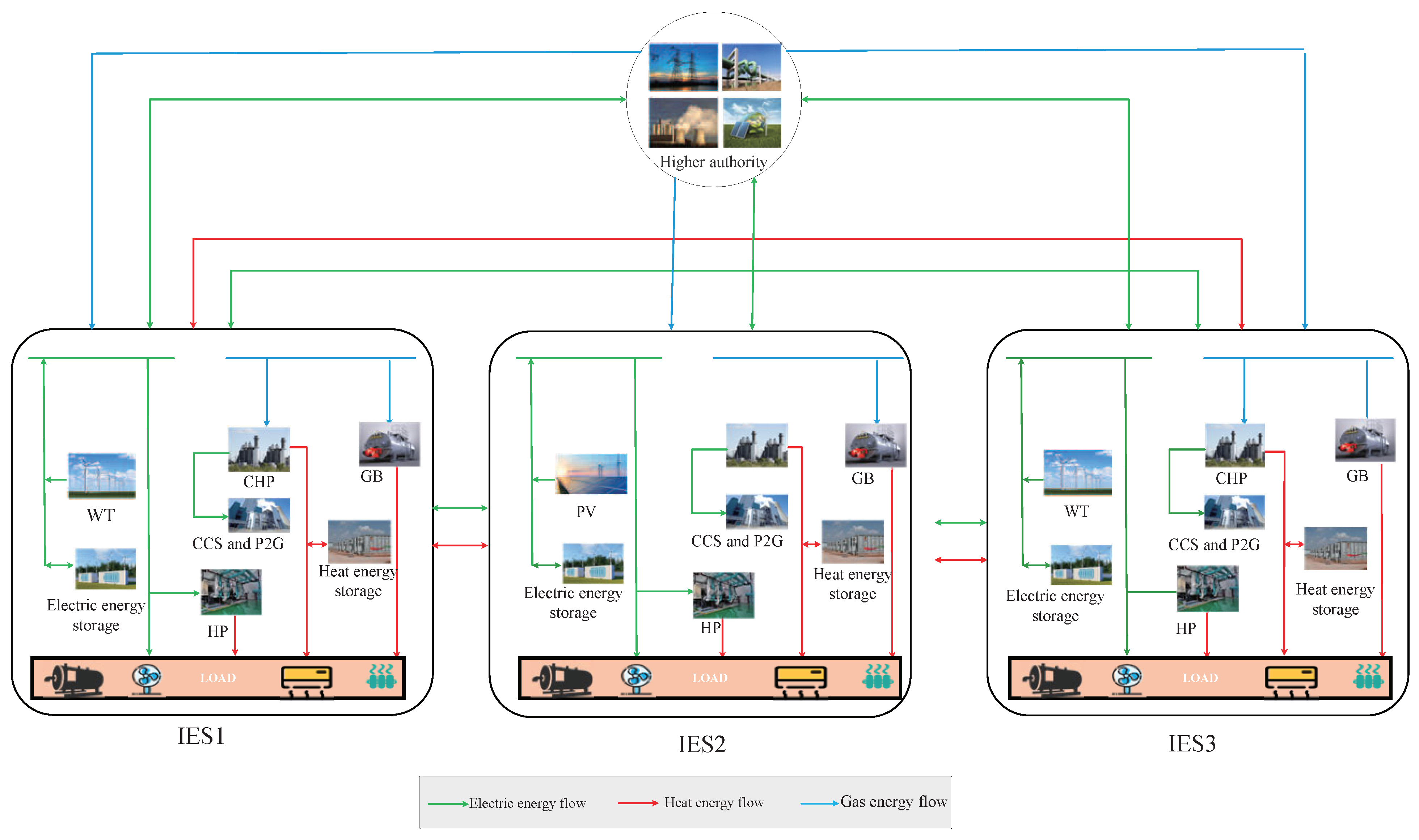
This paper presents an IoT-based architecture for energy sharing across multiple IESs, as shown in Figure 1. Each IES has an independent energy trading port and exchanges information via these ports using wireless communication technology to fully protect individual privacy. In the diagram, lines of different colors represent various types of energy, illustrating how each IES can share electrical and heat energies with others, thereby enhancing the system’s flexibility and ensuring a reliable supply–demand balance. Additionally, according to [20], it is assumed that the core components of each IES include combined heat and power (CHP), gas boiler (GB), heat pump (HP), wind turbine (WT), photovoltaic (PV), energy storage, P2G, and carbon capture storage (CCS). The energy storage can store both electrical and heat energies, improving the system’s flexibility in adapting to load fluctuations. The CCS can capture ${\mathrm{CO}}_2$ emissions from CHP and use them in P2G, thereby reducing reliance on external natural gas. This model not only significantly improves the system’s efficiency and economy but also considers the goal of low-carbon development.

Figure 1. The energy trading structure among IESs.

2.1. Model Constraints

(1)

CHP model.

The constraints for CHP are as follows:

$$\left\{\begin{array}{cc}\hfill & P_t^{\mathrm{CHP}}={\eta }_1{P}_t^{\mathrm{CHP},\mathrm{g}}\hfill \\ \hfill & H_t^{\mathrm{CHP}}={\eta }_2{P}_t^{\mathrm{CHP},\mathrm{g}}\hfill \\ \hfill & 0\le P_t^{\mathrm{CHP}}\le P_{\max }^{\mathrm{CHP}}\hfill \\ \hfill & 0\le H_t^{\mathrm{CHP}}\le H_{\max }^{\mathrm{CHP}}\hfill \end{array}\right.$$

(1)

where ${\eta }_1$, ${\eta }_2$ are the energy efficiency. $P_{\max }^{\mathrm{CHP}}$ and $H_{\max }^{\mathrm{CHP}}$ are the upper limits of the energy output. $P_t^{\mathrm{CHP},\mathrm{g}}$ is the natural gas power consumed at period t. $P_t^{\mathrm{CHP}}$ and $H_t^{\mathrm{CHP}}$ are the electrical energy and heat energy outputs at period t, respectively.

(2)

GB model.

The constraints for GB are as follows:

$$\left\{\begin{array}{cc}\hfill & H_t^{\mathrm{GB}}={\eta }_3{P}_t^{\mathrm{GB},\mathrm{g}}\hfill \\ \hfill & 0\le H_t^{\mathrm{GB}}\le H_{\max }^{\mathrm{GB}}\hfill \end{array}\right.$$

(2)

where ${\eta }_3$ is the energy efficiency. $P_t^{\mathrm{GB},\mathrm{g}}$ is the natural gas power consumed at period t. $H_{\max }^{\mathrm{GB}}$ is the upper limit of heat energy output. $H_t^{\mathrm{GB}}$ is the heat energy output at period t

(3)

HP model.

The constraints for HP are as follows:

$$\left\{\begin{array}{cc}\hfill & H_t^{\mathrm{HP}}={\eta }_4{P}_t^{\mathrm{HP}}\hfill \\ \hfill & 0\le H_t^{\mathrm{HP}}\le H_{\max }^{\mathrm{HP}}\hfill \end{array}\right.$$

(3)

where $H_t^{\mathrm{HP}}$ and $P_t^{\mathrm{HP}}$ are the heat/electrical energy output/consumed at period t. ${\eta }_4$ is the energy efficiency. $H_{\max }^{\mathrm{HP}}$ is the upper limit of heat energy output.

(4)

Energy trading with the grid model.

$$\left\{\begin{array}{cc}\hfill & 0\le P_t^{\mathrm{buy}}\le u_t^{\mathrm{buy}}{P}_{\max }^{\mathrm{buy}}\hfill \\ \hfill & 0\le P_t^{\mathrm{sell}}\le u_t^{\mathrm{sell}}{P}_{\max }^{\mathrm{sell}}\hfill \\ \hfill & u_t^{\mathrm{buy}}+u_t^{\mathrm{sell}}\le 1\hfill \end{array}\right.$$

(4)

where $P_{\max }^{\mathrm{buy}}$, $P_{\max }^{\mathrm{sell}}$ are the upper limits of electrical energy traded with the grid, respectively. $u_t^{\mathrm{buy}}$ and $u_t^{\mathrm{sell}}$ are binary state variables at period t. $P_t^{\mathrm{buy}}$ and $P_t^{\mathrm{sell}}$ are the purchases and sales of electrical energy at period t, respectively.

(5)

Energy storage model.

$$\left\{\begin{array}{cc}\hfill & 0\le P_t^{\mathrm{dis}}\le u_t^{\mathrm{e},\mathrm{dis}}{P}_{max}\hfill \\ \hfill & 0\le P_t^{\mathrm{ch}}\le u_t^{\mathrm{e},\mathrm{ch}}{P}_{max}\hfill \\ \hfill & E_t^{\mathrm{e}}=E_{t-1}^{\mathrm{h}}+{\eta }_{\mathrm{e},\mathrm{ch}}{P}_t^{\mathrm{ch}}-P_t^{\mathrm{dis}}/{\eta }_{\mathrm{e},\mathrm{dis}}\hfill \\ \hfill & u_t^{\mathrm{e},\mathrm{ch}}+u_t^{\mathrm{e},\mathrm{dis}}\le 1\hfill \end{array}\right.$$

(5)

$$\left\{\begin{array}{cc}\hfill & 0\le H_t^{\mathrm{dis}}\le u_t^{\mathrm{h},\mathrm{dis}}{H}_{max}\hfill \\ \hfill & 0\le H_t^{\mathrm{ch}}\le u_t^{\mathrm{h},\mathrm{ch}}{H}_{max}\hfill \\ \hfill & E_t^{\mathrm{h}}=E_{t-1}^{\mathrm{h}}+{\eta }_{\mathrm{h},\mathrm{ch}}{H}_t^{\mathrm{ch}}-H_t^{\mathrm{dis}}/{\eta }_{\mathrm{h}\mathrm{dis}}\hfill \\ \hfill & u_t^{\mathrm{h},\mathrm{ch}}+u_t^{\mathrm{h},\mathrm{dis}}\le 1\hfill \end{array}\right.$$

(6)

where $P_{\max }$, $H_{\max }$ are the upper limits of charging and discharging power. ${\eta }_{\mathrm{e},\mathrm{ch}}$, ${\eta }_{\mathrm{e},\mathrm{dis}}$, ${\eta }_{\mathrm{h},\mathrm{ch}}$, ${\eta }_{\mathrm{h},\mathrm{dis}}$ are the efficiency. $E_t^{\mathrm{e}}$ and $E_t^{\mathrm{h}}$ are the capacity at period t. $u_t^{\mathrm{e},\mathrm{ch}}$, $u_t^{\mathrm{e},\mathrm{dis}}$, $u_t^{\mathrm{h},\mathrm{ch}}$, $u_t^{\mathrm{h},\mathrm{dis}}$ are binary state variables at period t. $P_t^{\mathrm{ch}}$, $P_t^{\mathrm{dis}}$, $H_t^{\mathrm{ch}}$, $H_t^{\mathrm{dis}}$ are the charging and discharging power of the energy storage at period t, respectively.

(6)

CCS and P2G model

The constraints for a CCS and P2G are as follows:

$$\left\{\begin{array}{cc}\hfill & P_t^{\mathrm{CCS}}={\eta }^{\mathrm{CCS}}{C}_t^{\mathrm{CCS}},\hfill \\ \hfill & G_t^{\mathrm{C}{\mathrm{H}}_4}={\displaystyle \frac{{\eta }^{\mathrm{P}2\mathrm{G}}{P}_t^{\mathrm{P}2\mathrm{G}}}{H_g}},\hfill \\ \hfill & C_t^{\mathrm{CCS}}={\lambda }^{{\mathrm{CO}}_2}{P}_t^{\mathrm{P}2\mathrm{G}},\hfill \\ \hfill & 0\le P_t^{\mathrm{CCS}}\le P_{max}^{\mathrm{CCS}},\hfill \\ \hfill & 0\le P_t^{\mathrm{P}2\mathrm{G}}\le P_{max}^{\mathrm{P}2\mathrm{G}}\hfill \end{array}\right.$$

(7)

where $P_t^{\mathrm{CCS}}$ and $P_t^{\mathrm{P}2\mathrm{G}}$ are the electrical energy consumed by a CCS and P2G at period t, respectively. $C_t^{\mathrm{CCS}}$ is ${\mathrm{CO}}_2$ captured by CCS at period t. ${\eta }^{\mathrm{CCS}}$, ${\eta }^{\mathrm{P}2\mathrm{G}}$, and ${\lambda }^{{\mathrm{CO}}_2}$ are the efficiency. $G_t^{{\mathrm{CH}}_4}$ is ${\mathrm{CH}}_4$ produced at period t. $P_{\max }^{\mathrm{CCS}}$ and $P_{\max }^{\mathrm{P}2\mathrm{G}}$ are the upper limits of electrical energy consumed by a CCS and P22G at period t, respectively.

(7)

Power balance constraint

The constraints for power balance are as follows:

$$\left\{\begin{array}{cc}\hfill P_t^{\mathrm{CHP}}+P_t^{\mathrm{WT}}+P_t^{\mathrm{PV}}+P_t^{\mathrm{ch}}+P_t^{\mathrm{buy}}& =P_t^{\mathrm{load}}+P_t^{\mathrm{dis}}+P_t^{\mathrm{sell}}+P_t^{\mathrm{CCS}}+P_t^{\mathrm{P}2\mathrm{G}}+P_{ij,t}\hfill \\ \hfill H_t^{\mathrm{CHP}}+H_t^{\mathrm{GB}}+H_t^{\mathrm{HP}}+H_t^{\mathrm{dis}}& =H_t^{\mathrm{load}}+H_t^{\mathrm{ch}}+H_{ij,t}\hfill \end{array}\right.$$

(8)

where $P_t^{\mathrm{WT}}$ and $P_t^{\mathrm{PV}}$ are the WT and PV power at period t, respectively. $P_{ij,t}$ and $H_{ij,t}$ are the energy trading volumes among IESs at period t.

2.2. Objective Function

For a single IES, the objective function is to minimize the operating cost $C^{\mathrm{obj}}$. It includes the equipment start-up and shutdown costs $C^1$, electricity purchase and sale cost $C^2$, natural gas purchase cost $C^3$, and energy storage operation cost $C^4$ as follows:

$$C^{\mathrm{obj}}=min(C^1+C^2+C^3+C^4)$$

(9)

$$\left\{\begin{array}{c}{C}^1={\displaystyle \sum _{t=1}^T}g(u_t^{\mathrm{e},\mathrm{ch}}+u_t^{\mathrm{e},\mathrm{dis}}+u_t^{\mathrm{h},\mathrm{ch}}+u_t^{\mathrm{h},\mathrm{dis}}),\hfill \\ C^2={\displaystyle \sum _{t=1}^T}{r}_t^{\mathrm{buy}}{P}_t^{\mathrm{buy}}-r_t^{\mathrm{sell}}{P}_t^{\mathrm{sell}},\hfill \\ C^3={\displaystyle \sum _{t=1}^T}{c}_{\mathrm{gas}}·(G_t^{\mathrm{CHP}}+G_t^{\mathrm{GB}}-G_t^{\mathrm{C}{\mathrm{H}}_4})\hfill \\ C^4={\displaystyle \sum _{t=1}^T}{\xi }_{\mathrm{e}}·\left(P_t^{\mathrm{ch}}+P_t^{\mathrm{dis}}\right)+{\xi }_{\mathrm{h}}·\left(H_t^{\mathrm{ch}}+H_t^{\mathrm{dis}}\right)\hfill \end{array}\right.$$

(10)

where g and $c_{\mathrm{gas}}$ are the prices of energy storage behavior and natural gas. $r_t^{\mathrm{sell}}$, $r_t^{\mathrm{buy}}$ are the prices of the grid. ${\xi }_{\mathrm{e}}$ and ${\xi }_{\mathrm{h}}$ are the prices of the energy storage operation.

3. Development and Solution of Four-Level Robust Optimization Model

This section introduces a multi-interval uncertainty set to describe the fluctuation of renewable energy. To address this uncertainty, a four-level robust optimization model for IES is established.

3.1. Construction of Uncertainty Set

The traditional uncertainty set is shown as follows:

$$U=\left\{\begin{array}{c}{u}^w=\left[P_t^{\mathrm{WT}},P_t^{\mathrm{PV}}\right]\in {\mathbb{R}}^{\left(T\right)\times 2}\hfill \\ u_t^w=u_t^{w,*}+u_t^{w,+}{\epsilon }_t^{w,+}-u_t^{w,-}{\epsilon }_t^{w,-}\hfill \\ \left({\epsilon }_t^{w,+}+{\epsilon }_{w,t}^{w,-}\right)\le 1,\hfill \\ \sum _{t=1}^T({\epsilon }_t^{w,+}+{\epsilon }_t^{w,+})\le {\Gamma }^w\hfill \end{array}\right.$$

(11)

where ${\epsilon }_t^{w,+}$ and ${\epsilon }_t^{w,-}$ are binary state variables. ${\Gamma }^w$ is the robustness budget.

From (11), it is evident that the uncertainty of renewable energy always appears at the boundaries of the interval, which does not align with the actual situation. To reduce conservatism, this paper employs a multi-interval uncertainty set to describe the fluctuation range of renewable energy, as detailed below:

$$U=\left\{\begin{array}{c}{u}^w=\left[P_t^{\mathrm{WT}},P_t^{\mathrm{PV}}\right]\in {\mathbb{R}}^{\left(T\right)\times 2},u_t^w=u_t^{w,*}+{\displaystyle \sum _{a=1}^{N_a}}\left(u_t^{w,a+}{\epsilon }_t^{w,a+}-u_t^{w,a-}{\epsilon }_t^{w,a-}\right),\hfill \\ 0\le {\epsilon }_t^{w,a\pm }\le 1,0\le {\displaystyle \sum _{a=1}^{N_{\mathrm{a}}}}\left({\epsilon }_t^{w,a+}+{\epsilon }_t^{w,a-}\right)\le 1,{\displaystyle \sum _{t=1}^T}\left({\epsilon }_t^{w,a+}+{\epsilon }_t^{w,a-}\right)\le {\Gamma }^w,\hfill \\ {\displaystyle \sum _{t=1}^T}{\displaystyle \sum _{a=1}^{N_a}}{\epsilon }_t^{w,a+}={\displaystyle \sum _{t=1}^T}{\displaystyle \sum _{a=1}^{N_{\mathrm{a}}}}{\epsilon }_t^{w,a-},-\Lambda \le {\displaystyle \frac{{\displaystyle \sum _{t=1}^T}{\displaystyle \sum _{a=1}^{N_{\mathrm{a}}}}\left(u_t^{w,a+}{\epsilon }_t^{w,a+}-u_t^{w,a-}{\epsilon }_t^{w,a-}\right)}{{\displaystyle \sum _{t=1}^T}{u}_t^{w,*}}}\le \Lambda ,{\displaystyle \frac{{\Gamma }^{w+1,a}}{{\Gamma }^{w,a}}}={\displaystyle \frac{P^{w+1,a}}{P^{w,a}}}\hfill \end{array}\right\}$$

(12)

From (12), it is evident that the entire single interval is divided into $N_a$ multiple intervals. Within any given period t, the uncertainty can only exhibit one deviation value within these $N_a$ intervals. Notably, the multi-interval uncertainty set proposed in this paper differs from that in [21] by taking distributional balance into account. It ensures that the sum of positive deviations is equal to the sum of negative deviations over the entire scheduling period, and that the total deviation is constrained within [$-\Lambda$, $\Lambda$].

To avoid extreme cases of the uncertainty set, this paper establishes an uncertainty set based on the initial probability distribution, using a combined norm that includes both 1-norm and ∞-norm as constraints to restrict the deviation of probability. The details are as follows:

$$\Omega =\left\{\left\{p_s\right\}\left|\begin{array}{c}{p}_s\ge 0,s=1,2,\cdots N_s\hfill \\ {\displaystyle \sum _{s=1}^{N_s}}{p}_s=1\hfill \\ {\displaystyle \sum _{s=1}^{N_s}}\left|p_s-p_{s,0}\right|\le {\theta }_1\hfill \\ \underset{1\le s\le N_s}{max}\left|p_s-p_{s,0}\right|\le {\theta }_{\infty }\hfill \end{array}\right.\right\}$$

(13)

where $p_s$ and $p_{s,0}$ are the probability distribution values of the actual scenario and the initial scenario, respectively. ${\theta }_1$ and ${\theta }_{\infty }$ represent the allowable deviations for the 1-norm and $\theta$-norm probabilities, respectively.

3.2. Four-Level Robust Model

Based on the uncertainty sets described above, the four-level robust optimization model for the IES is formulated as follows:

$$\left\{\begin{array}{c}\underset{\mathit{x}}{min}{C}^1+\underset{{\mathit{p}}_s\in \Omega }{max}\underset{\mathit{u}\in \mathit{U}}{max}\underset{\mathit{y}\in \Pi \left(\mathit{x},\mathit{p},\mathit{u}\right)}{min}{\displaystyle \sum _{s=1}^{N_s}}{\mathit{p}}_s\left(C^2+C^3+C^4\right)\hfill \\ \mathrm{s}.\mathrm{t}\left(1\right)-\left(8\right),\left(12\right)-\left(13\right)\hfill \end{array}\right.$$

(14)

For ease of description, (14) can be expressed as follows:

$$\left\{\begin{array}{c}\underset{\mathit{x}}{min}{c}^{\mathrm{T}}x+\underset{{\mathit{p}}_s\in \Omega }{max}\underset{\mathit{u}\in \mathit{U}}{max}\underset{\mathit{y}\in \Pi \left(\mathit{x},\mathit{y},\mathit{u}\right)}{min}{\displaystyle \sum _{s=1}^{N_s}}{\mathit{p}}_s\left(d^{\mathrm{T}}y\right)\hfill \\ st.\mathit{Bx}+\mathit{Cy}\le \mathit{f}\hfill \\ \Pi \left(\mathit{x},\delta ,\mathit{u}\right)=\left\{\mathit{y}\left|\mathit{Dx}+\mathit{Ey}\le \mathit{g}-\mathit{K}\mathit{u}\right.\right\}\hfill \\ \Omega =\left\{{\mathit{p}}_s\left|\mathit{F}{\mathit{p}}_s\le \mathit{h}\right.\right\},\mathit{U}=\left\{\mathit{u}\left|\mathit{Gu}\le \mathit{k}\right.\right\},\mathit{x}\in \left\{0,1\right\}\hfill \end{array}\right.$$

(15)

where $\mathit{x}$ and $\mathit{y}$ are decision vectors. $\mathit{B}$, $\mathit{C}$, $\mathit{D}$, $\mathit{E}$, $\mathit{F}$, $\mathit{G}$, $\mathit{f}$, $\mathit{g}$, $\mathit{k}$, $\mathit{d}$ are constant coefficients matrices.

3.3. Solution Method

The C&CG algorithm is utilized in this paper to decompose (15) into a master problem and a subproblem, which are solved iteratively to ensure convergence accuracy. The detailed solution steps are as follows:

(1)

Master problem

The master problem determines the operational states of IES devices based on the worst-case scenarios transmitted from the subproblem, as detailed below:

$$\left\{\begin{array}{c}\underset{\mathit{x}}{min}{\mathit{c}}^{\mathrm{T}}\mathit{x}+\mathit{\eta }\hfill \\ st.\mathit{Bx}+\mathit{Cy}\le \mathit{f},\mathit{Dx}+\mathit{E}{\mathit{y}}^l\le \mathit{g}-\mathit{K}{\mathit{u}}_l\hfill \\ \mathit{\eta }\ge {\displaystyle \sum _{s=1}^{N_s}}{p}_s^{*}\left(d^{\mathrm{T}}{\mathbf{y}}_l\right),\hfill \\ \mathit{\eta }\ge 0,\mathit{x}\in \left\{0,1\right\},\forall 1\le l\le L\hfill \end{array}\right.$$

(16)

where $\mathit{\eta }$ is an auxiliary variable.

(2)

Subproblem

The subproblem aims to identify the worst-case scenario and pass it to the master problem, as detailed below:

$$\left\{\begin{array}{c}\underset{p_s\in \Omega }{max}\underset{\mathit{u}\in U}{max}\underset{\mathit{y}\in \Pi \left(\mathit{x},\delta ,u\right)}{min}{\displaystyle \sum _{k=1}^{N_s}}{p}_s\left(d^{\mathrm{T}}\mathit{y}\right)\hfill \\ st.\mathit{D}{\mathit{x}}^{*}+\mathbf{Fy}\le \mathit{g}-\mathit{K}\mathit{u},\hfill \\ \mathit{F}{\mathit{p}}_k\le \mathit{g},\mathit{Gu}\le \mathit{k}\hfill \end{array}\right.$$

(17)

Notably, the subproblem contains two continuous variables, which makes solving the problem more challenging if computed simultaneously. To address this, it is divided into two separate subproblems, solved through the AIS algorithm. The specific details are as follows:

(a)

$p_s$-fixed bi-lever subproblem (SP1)

$$\mathrm{S}{\mathrm{P}}_1:\left\{\begin{array}{c}\underset{\mathit{u}\in \mathit{U}}{max}\underset{\mathit{y}\in \Pi \left(\mathit{x},\delta ,\mathit{u}\right)}{min}{\displaystyle \sum _{k=1}^K}{p}_s^{*}\left(d^{\mathrm{T}}\mathbf{y}\right)\hfill \\ st.\mathit{D}{\mathit{x}}^{*}+\mathit{Fy}\le g-\mathit{K}\mathit{u},\hfill \\ \mathit{Gu}\le \mathit{k}\hfill \end{array}\right.$$

(18)

Since the model is linear, the Karush–Kuhn–Tucker (KKT) conditions can be used to convert it into a single-level model as follows:

$$\left\{\begin{array}{c}\underset{\mathit{u}\in U,\mathbf{y}\in \Pi \left(\mathit{x},\mathit{p},\mathit{u}\right)}{max}{\displaystyle \sum _{s=1}^{N_s}}{\mathit{p}}_s^{*}\left(d^{\mathrm{T}}\mathit{y}\right)\hfill \\ st.\mathit{D}{\mathit{x}}^{*}+\mathit{Fy}\le g-\mathit{Ku}\hfill \\ 0\le \mathit{Gu}-\mathit{k}\hfill \\ {\mathit{\xi }}^{\mathrm{T}}\mathit{D}+p_s^{*}\left(d^{\mathrm{T}}\right)=0,\hfill \\ 0\le \mathit{\xi }\le M\left(1-\delta \right)\hfill \\ M\delta \le \mathit{g}-\mathit{Ku}-\mathit{D}{\mathit{x}}^{*}-\mathit{Ey}\hfill \end{array}\right.$$

(19)

where $\mathit{\xi }$ is a dual variable corresponding to the constraints. $\mathrm{M}$ is introduced as a very large positive number. $\delta$ is a binary variable.

By solving (19), the optimal solution of SP1 can be determined.

(b)

u-fixed bi-level subproblem (SP2):

$$\left\{\begin{array}{c}\underset{{\mathit{p}}_s\in \Omega }{max}\underset{\mathit{y}\in \Pi \left(\mathit{x},\mathit{p},\mathit{u}\right)}{min}{\displaystyle \sum _{s=1}^{N_s}}{\mathit{p}}_s\left(d^{\mathrm{T}}\mathit{y}\right)\hfill \\ st.\mathit{D}{\mathit{x}}^{*}+\mathit{Ey}\le \mathit{g}-\mathit{Ku},\hfill \\ \mathit{E}{\mathit{p}}_s\le \mathit{g}\hfill \end{array}\right.$$

(20)

Although the objective function contains a nonlinear term involving the product of $p_s$ and y, SP2 does not require transformation using the KKT conditions. Since $p_s$ and y are independent, SP2 can be split into distinct independent linear programming problems.

$$\left\{\begin{array}{c}{l}_s^{*}=min{\mathit{d}}^T{\mathit{y}}^s,s=1,\cdots N_s\hfill \\ st.\mathit{E}{\mathit{p}}_s\le \mathit{g}\hfill \end{array}\right.$$

(21)

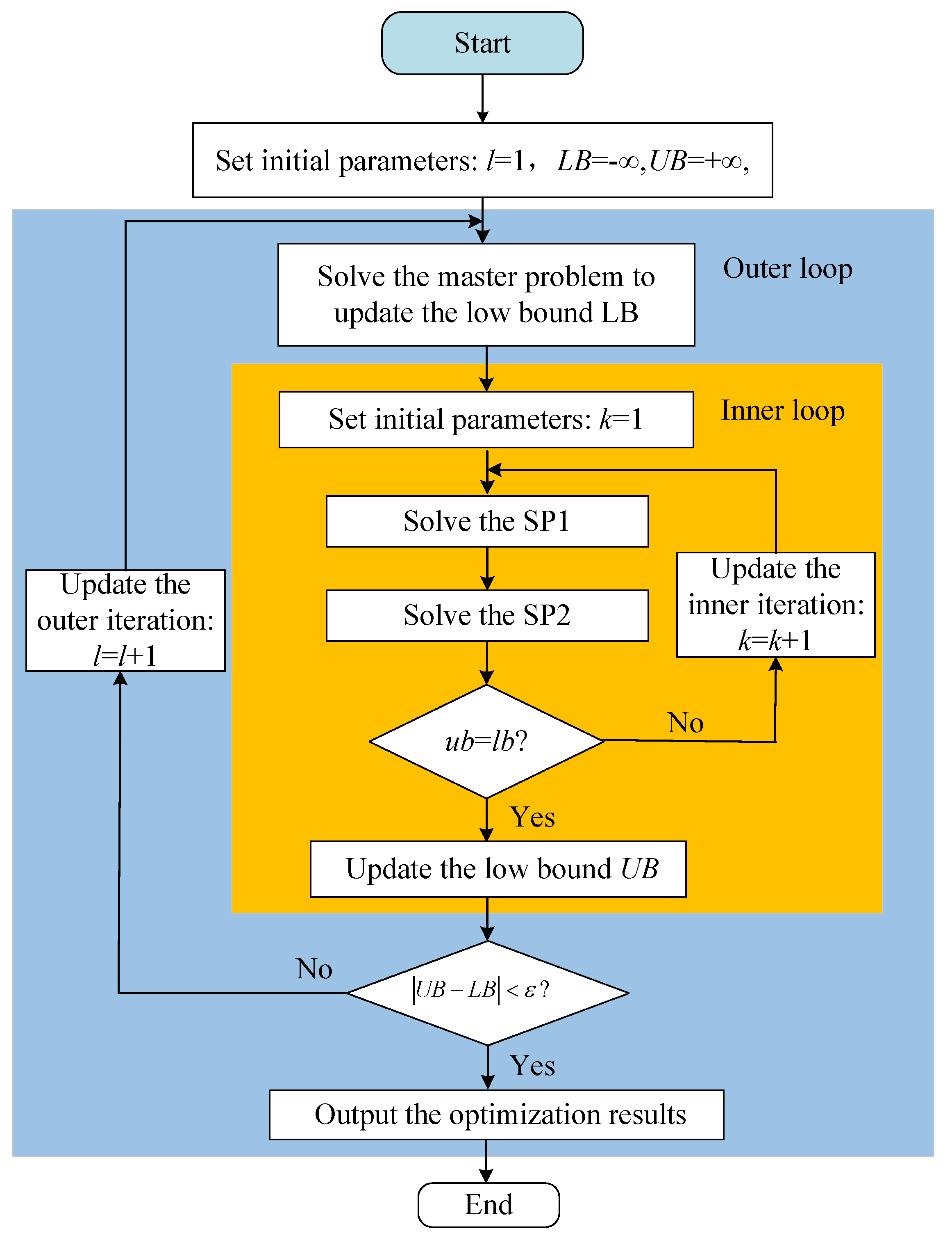
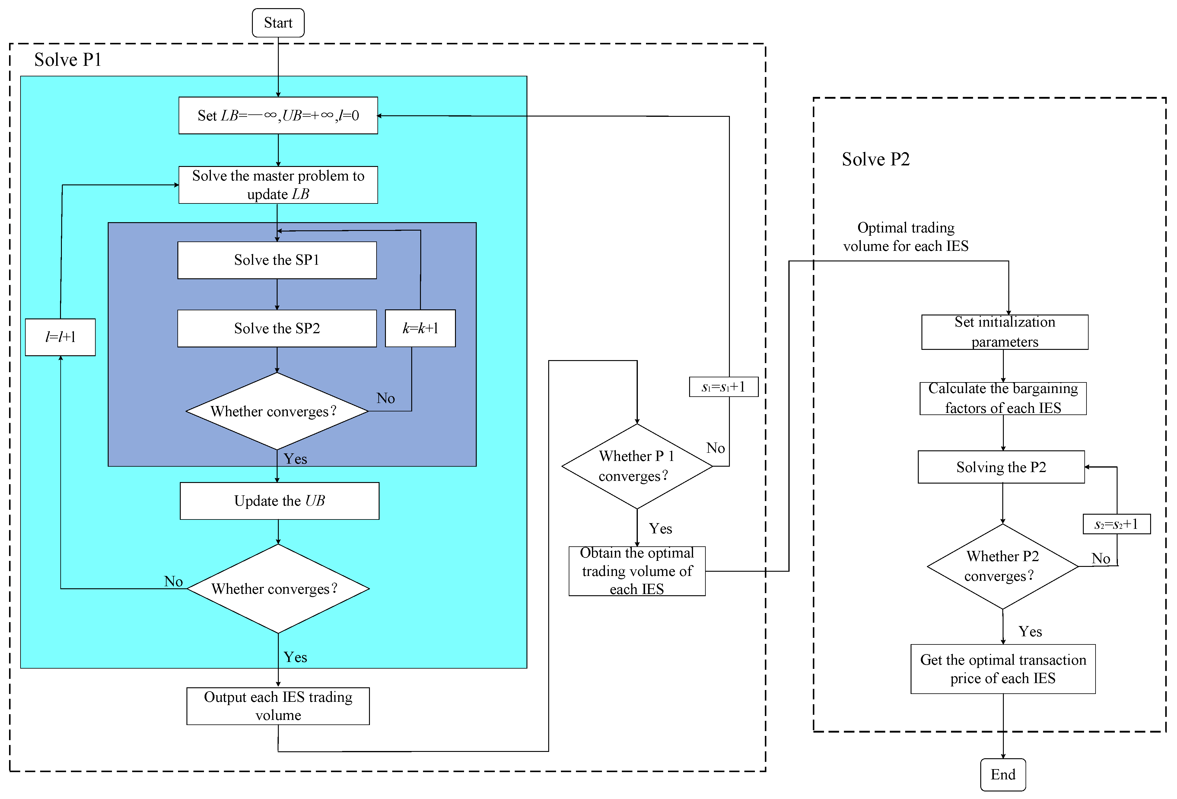
The solving process of the four-level robust model is shown in Figure 2. Firstly, establish a multi-interval uncertainty set. Then, the outer loop utilizes the C&CG algorithm to optimize decision variables and passes them to the inner loop. Finally, the inner loop applies the AIS algorithm to iteratively determine and relay worst-case scenarios along with renewable energy probabilities back to the outer loop.

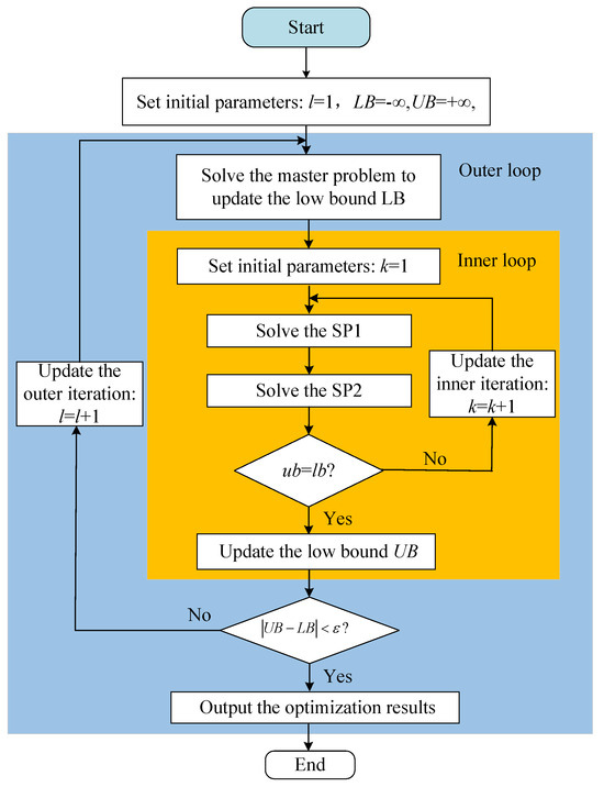
Figure 2. Four-level robust model-solving process.

4. Establishment and Solution of Cooperative Model

In this paper, it is assumed that each IES is an independent subject that wishes to maximize its benefits through cooperation. However, in the process of cooperation, various factors affect the bargaining power of each subject. Therefore, the Nash–Harsanyi bargaining model is established to ensure an equitable distribution of benefits among IESs.

4.1. Model Establishment

Generally, the structure of the Nash–Harsanyi bargaining model is as follows:

$$\left\{\begin{array}{c}max{\displaystyle \prod _{i=1}^I}{(C_i^0-C_i)}^{T{P}_i}\hfill \\ \mathrm{s}.\mathrm{t}{C}_i^0\ge C_i\hfill \end{array}\right.$$

(22)

where $C_i^0$ and $C_i$ are the costs before and after cooperation, respectively. $T{P}_i$ is the bargaining power.

4.2. Equivalent Model

Equation (22) is a non-linear optimization problem. To solve it, we need to carry out an equivalent transformation. The specific method is to decompose it into two subproblems and solve them step-by-step. The two subproblems are represented as follows:

P1: Cost optimization subproblem.

$$\left\{\begin{array}{cc}\hfill & \sum _{i=1}^I{C}_i^{\mathrm{IES}}\hfill \\ \hfill & \mathrm{s}.\mathrm{t}.P_{min}\le P_{ij,t}\le P_{max},\hfill \\ \hfill & H_{min}\le H_{ij,t}\le H_{max},\hfill \\ \hfill & \left(1\right)–\left(8\right),\left(12\right)–\left(13\right)\hfill \end{array}\right.$$

(23)

where $P_{min}$, $P_{max}$, $H_{min}$, and $H_{max}$ are upper and lower limits of energy trading. When multiple energy tradings are considered, the operating cost of each IES $C_i^{\mathrm{IES}}$ is as follows:

$$C_i^{\mathrm{IES}}=min(C_i^1+C_i^2+C_i^3+C_i^4-C_i^5)$$

(24)

$$C_i^5=\sum _{i=1}^I\sum _{j\in I\setminus \left\{i\right\}}^I\sum _{t=1}^T\left(r_{ij,t}^{\mathrm{e}}{P}_{ij,t}+r_{ij,t}^{\mathrm{h}}{H}_{ij,t}\right)$$

(25)

where $C_i^5$ is the cost of energy trading. $r_{ij,t}^{\mathrm{e}}$ and $r_{ij,t}^{\mathrm{h}}$ are energy negotiation prices at period t, respectively.

P2: The payment subproblem.

$$\left\{\begin{array}{cc}\hfill & max\prod _{i=1}^I{\left(C_i^0-C_i^{\mathrm{IES}’}+C_i^{\mathrm{trade}}\right)}^{{\mathrm{TP}}_i}\hfill \\ \hfill & \mathrm{s}.\mathrm{t}.r_{min}^{\mathrm{e}}\le r_{ij,t}^{\mathrm{e}}\le r_{max}^{\mathrm{e}},\hfill \\ \hfill & r_{min}^{\mathrm{h}}\le r_{ij,t}^{\mathrm{h}}\le r_{max}^{\mathrm{h}},\hfill \\ \hfill & C_i^0\ge C_i^{\mathrm{IES}’}+C_i^{\mathrm{trade}}\hfill \end{array}\right.$$

(26)

where $r_{min}^{\mathrm{e}}$, $r_{max}^{\mathrm{e}}$, $r_{min}^{\mathrm{h}}$, and $r_{max}^{\mathrm{h}}$ are upper and lower limits of energy trading negotiation price. $C_i^{\mathrm{IES}’}$ is the optimal solution obtained in P1.

In (26), the bargaining power of each IES is quantified based on two factors: the marginal contribution rate and the energy trading contribution rate.

(1)

Marginal contribution rate:

$$S_i^1={\displaystyle \frac{\left|C_i^0-C_i^{{\mathrm{IES}}^{\prime }}\right|}{\left|C_i^{{\mathrm{IES}}^{\prime }}\right|}}\times 100\%$$

(27)

(2)

Energy trading contribution rate:

$$S_i^2={\displaystyle \frac{1}{2}}·\left({\displaystyle \frac{\left|P_i^{\mathrm{p}2\mathrm{p}}\right|}{{\displaystyle \sum _i^I}\left|P_i^{\mathrm{p}2\mathrm{p}}\right|}}+{\displaystyle \frac{\left|H_i^{\mathrm{p}2\mathrm{p}}\right|}{{\displaystyle \sum _i^I}\left|H_i^{\mathrm{p}2\mathrm{p}}\right|}}\right)\times 100\%$$

(28)

where $P_i^{\mathrm{p}2\mathrm{p}}$ and $H_i^{\mathrm{p}2\mathrm{p}}$ are energy trading volumes.

Considering the two factors mentioned above, the total score for each participant can be obtained as follows:

$$S_i={\lambda }_1{S}_i^1+{\lambda }_2{S}_i^2$$

(29)

In (29), ${\lambda }_1$ and ${\lambda }_2$ represent the weights of IES in reflecting the bargaining power, and they satisfy ${\lambda }_1$ + ${\lambda }_2$ = 1. By normalizing the above equation, the $T{P}_i$ of each participant can be obtained.

$$T{P}_i={\displaystyle \frac{S_i}{{\displaystyle \sum _i^I}{S}_i}}$$

(30)

4.3. Model Solution Method

In order to protect the privacy of each IES, this paper uses the alternating direction method with multipliers (ADMM) algorithm to solve the model. First, (31) is introduced for decoupling:

$$P_{t,ij}+P_{t,ji}=0,H_{t,ij}+H_{t,ji}=0$$

(31)

Therefore, the augmented Lagrange function of P1 can be represented as follows:

$$\begin{array}{c}{L}_i={\displaystyle \sum _{i=1}^N}{C}_i^{\mathrm{IES}}+\hfill \\ {\displaystyle \sum _{i=1}^I}{\displaystyle \sum _{j\in I\setminus \left\{i\right\}}^I}{\displaystyle \sum _{t=1}^T}\left[{\lambda }_{t,ij}^{\mathrm{e}}(P_{t,ij}+P_{t,ji})+{\lambda }_{t,ij}^{\mathrm{h}}(H_{t,ij}+H_{t,ji})\right]+\hfill \\ {\displaystyle \sum _{i=1}^I}{\displaystyle \sum _{j\in I\setminus \left\{i\right\}}^I}{\displaystyle \sum _{t=1}^T}\left({\displaystyle \frac{{\rho }^{\mathrm{e}}}{2}}{∥P_{t,ij}+P_{t,ji}∥}_2^2+{\displaystyle \frac{{\rho }^{\mathrm{h}}}{2}}{∥H_{t,ij}+H_{t,ji}∥}_2^2\right)\hfill \end{array}$$

(32)

where ${\lambda }_{t,ij}^{\mathrm{e}}$ and ${\lambda }_{t,ij}^{\mathrm{e}}$ are Lagrange multipliers. ${\rho }^{\mathrm{e}}$ and ${\rho }^{\mathrm{h}}$ are penalty factors.

According to the ADMM algorithm, the distributed optimization model of IESi is expressed as follows:

$$\left\{\begin{array}{c}\underset{x}{min}\left(C^1+C^5\right)\hfill \\ +{\displaystyle \sum _{i=1}^I}{\displaystyle \sum _{j=I\setminus \left\{i\right\}}^I}{\displaystyle \sum _{t=1}^T}\left[{\lambda }_t^{\mathrm{e},ij}\left(P_{t,ij}+P_{t,ji}\right)+{\lambda }_t^{\mathrm{h},ij}\left(H_{t,ij}+H_{t,ji}\right)\right]\hfill \\ +{\displaystyle \sum _{i=1}^I}{\displaystyle \sum _{j=I\setminus \left\{i\right\}}^I}{\displaystyle \sum _{t=1}^T}\left({\displaystyle \frac{{\rho }^{\mathrm{e}}}{2}}{∥P_{t,ij}+P_{t,ji}∥}_2^2+{\displaystyle \frac{{\rho }^{\mathrm{h}}}{2}}{∥H_{t,ij}+H_{t,ji}∥}_2^2\right)\hfill \\ \underset{\Omega }{max}\underset{U}{max}\underset{y}{min}\left(C^2+C^3+C^4\right)\hfill \\ s.t.\left(1\right)–\left(8\right),\left(12\right)–\left(13\right)\hfill \end{array}\right.$$

(33)

By solving P1, substitute its optimal solution into P2 and solve. Then, introduce (34) to decouple P2:

$$r_{t,ij}^{\mathrm{e}}-r_{t,ji}^{\mathrm{e}}=0,r_{t,ij}^{\mathrm{h}}-r_{t,ji}^{\mathrm{h}}=0$$

(34)

Therefore, the augmented Lagrange function of P2 can be represented as follows:

$$\left\{\begin{array}{c}{L}_i^2=max{\displaystyle \prod _{i=1}^I}{\left(C_i^0-C_i^{{\mathrm{IES}}^{\prime }}+C_i^5\right)}^{\mathrm{T}{\mathrm{P}}_i}\hfill \\ +{\displaystyle \sum _{i=1}^I}{\displaystyle \sum _{j=I\setminus \left\{i\right\}}^I}{\displaystyle \sum _{t=1}^T}\left[{\zeta }_{t,ij}^{\mathrm{e}}\left(r_{t,ij}^{\mathrm{e}}-r_{t,ji}^{\mathrm{e}}\right)+{\zeta }_{t,ij}^{\mathrm{h}}\left(r_{t,ij}^{\mathrm{h}}-r_{t,ji}^{\mathrm{h}}\right)\right]\hfill \\ +{\displaystyle \sum _{i=1}^I}{\displaystyle \sum _{j=I\setminus \left\{i\right\}}^I}{\displaystyle \sum _{t=1}^T}\left({\displaystyle \frac{{\tau }^{\mathrm{e}}}{2}}{∥r_{t,ij}^{\mathrm{e}}-r_{t,ji}^{\mathrm{e}}∥}_2^2+{\displaystyle \frac{{\tau }^{\mathrm{h}}}{2}}{∥r_{t,ij}^{\mathrm{h}}-r_{t,ji}^{\mathrm{h}}∥}_2^2\right)\hfill \end{array}\right.$$

(35)

where ${\zeta }_{t,ij}^{\mathrm{e}}$ and ${\zeta }_{t,ij}^{\mathrm{e}}$ are Lagrange multipliers. ${\tau }^{\mathrm{e}}$ and ${\tau }^{\mathrm{h}}$ are penalty factors.

Similarly, the distributed optimization model of IESi is given as follows:

$$\left\{\begin{array}{c}max{\displaystyle \prod _{i=1}^I}{\left(C_i^0-C_i^{{\mathrm{IES}}^{\prime }}+C_i^5\right)}^{\mathrm{T}{\mathrm{P}}_i}\hfill \\ +{\displaystyle \sum _{i=1}^I}{\displaystyle \sum _{j=I\setminus \left\{i\right\}}^I}{\displaystyle \sum _{t=1}^T}\left[{\zeta }_{t,ij}^{\mathrm{e}}\left(r_{t,ij}^{\mathrm{e}}-r_{t,ji}^{\mathrm{e}}\right)+{\zeta }_{t,ij}^{\mathrm{h}}\left(r_{t,ij}^{\mathrm{h}}-r_{t,ji}^{\mathrm{h}}\right)\right]\hfill \\ +{\displaystyle \sum _{i=1}^I}{\displaystyle \sum _{j=I\setminus \left\{i\right\}}^I}{\displaystyle \sum _{t=1}^T}\left({\displaystyle \frac{{\tau }^{\mathrm{e}}}{2}}{∥r_{t,ij}^{\mathrm{e}}-r_{t,ji}^{\mathrm{e}}∥}_2^2+{\displaystyle \frac{{\tau }^{\mathrm{h}}}{2}}{∥r_{t,ij}^{\mathrm{h}}-r_{t,ji}^{\mathrm{h}}∥}_2^2\right)\hfill \\ s.t.C_i^0\ge C_i^{\mathrm{IES}}-C_i^{\mathrm{trade}}\hfill \end{array}\right.$$

(36)

The process of solving P1 and P2 using an the ADMM algorithm is shown in Appendix A.

In summary, the solution processes of the proposed strategy in this paper are presented in Figure 3. First, the C&CG-AIS algorithm is used to solve the four-level robust model of each IES. Then, the ADMM algorithm is employed to solve SP1. Once P1 meets the convergence criteria, the optimal transaction volume is transferred to P2, which then determines the optimal negotiation price for each IES.

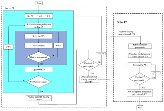
Figure 3. Flowchart of the proposed strategy solution.

5. Case Study

This section demonstrates the effectiveness of the proposed strategy through simulation.

5.1. Test System Description

Three typical IESs are used as examples to validate the proposed strategy through simulation analysis over a 24-h scheduling period. According to historical data, all IESs have a renewable energy output; the deviation ranges of WT and PV are defined as 10%, 15%, and 20%, respectively [22]. Additional parameter details are provided in Table 2.

Table 2. Specific parameters of IES.

Parameters	Value
${\eta }_1$,${\eta }_2$	0.35, 0.9
${\eta }_3$, ${\eta }_4$	0.9, 4.5
${\rho }^{\mathrm{e}}$, ${\rho }^{\mathrm{h}}$	0.01, 0.01
${\tau }^{\mathrm{e}}$, ${\tau }^{\mathrm{h}}$	100, 100
$P_{\max }^{\mathrm{CHP}}$	2500
$H_{\max }^{\mathrm{CHP}}$	2500
$H_{\max }^{\mathrm{HP}}$	1000
$H_{\max }^{\mathrm{GB}}$	2000
$c_{gas}$	2.7
${\xi }_{\mathrm{e}}$, ${\xi }_{\mathrm{h}}$	0.4, 0.2
g	0.1
${\eta }^{\mathrm{CCS}}$, ${\eta }^{\mathrm{P}2\mathrm{G}}$	0.5, 0.55

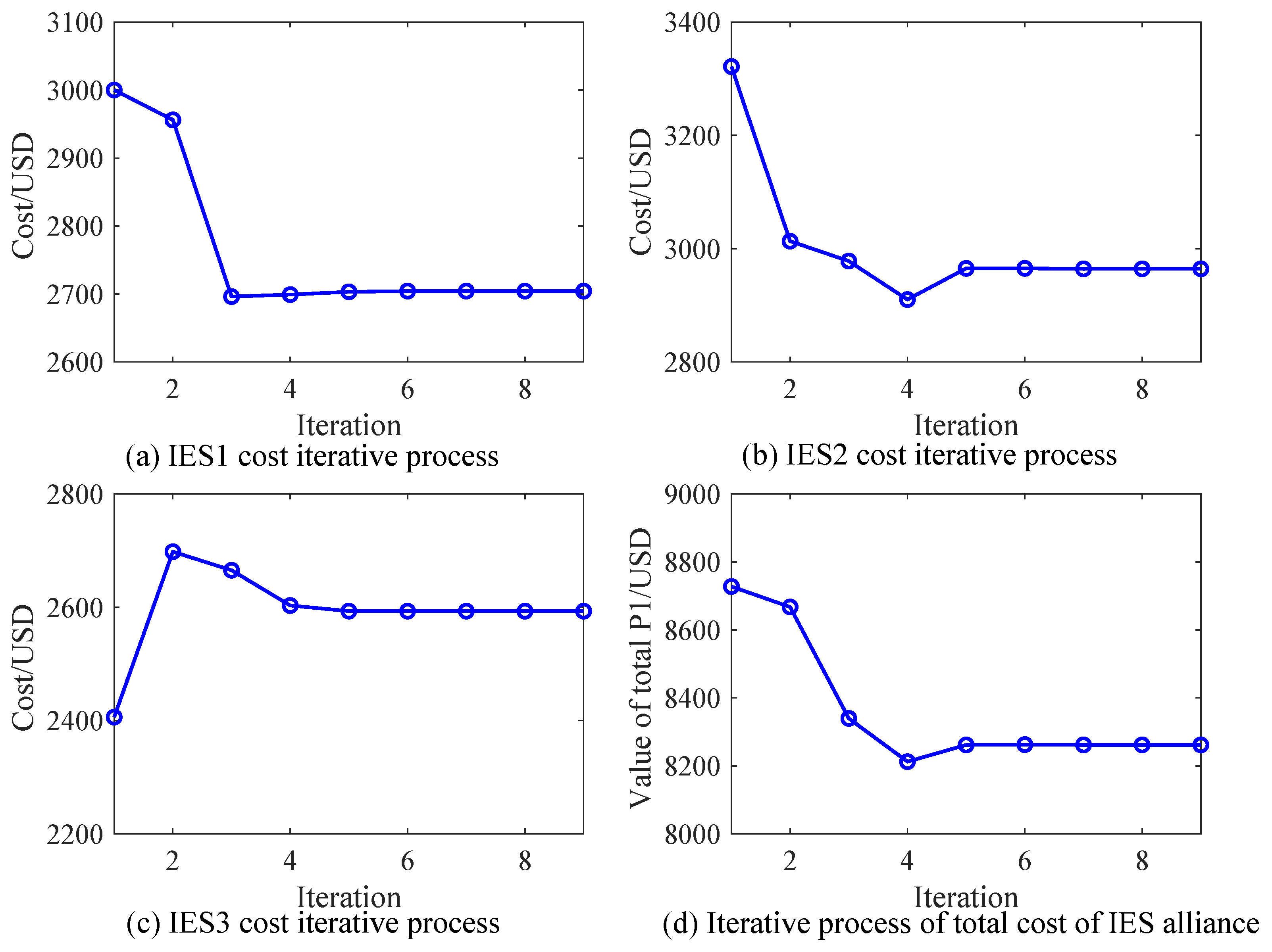
5.2. Algorithm Convergence Analysis

The convergence process of P1 and P2 for each IES is illustrated in Figure 4 and Figure 5.

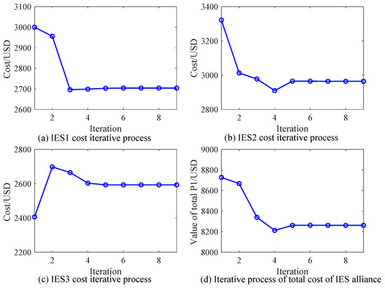
Figure 4. The iterative convergence result of P1.

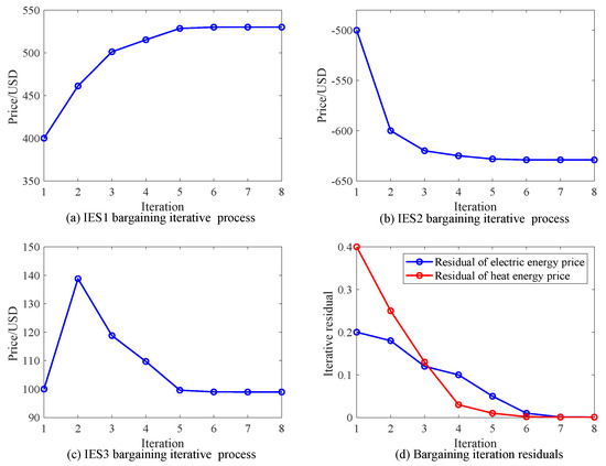
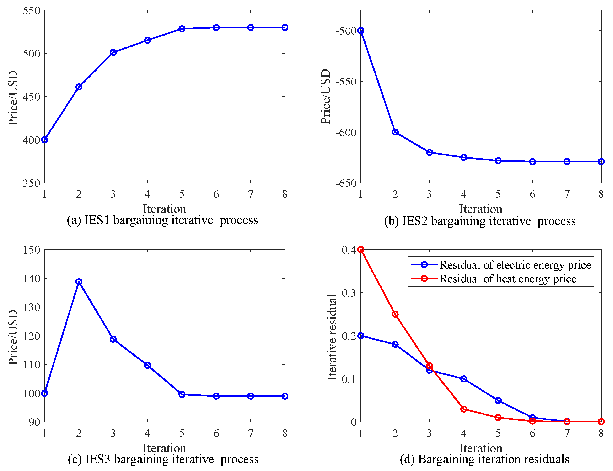
Figure 5. The iterative convergence result of P2.

Figure 4 shows that convergence is achieved after the 9th iteration in P1, while Figure 5 indicates convergence after the 8th iteration in P2. These results demonstrate that the proposed solution method ensures rapid model convergence.

5.3. Optimization Results of Nash Bargaining

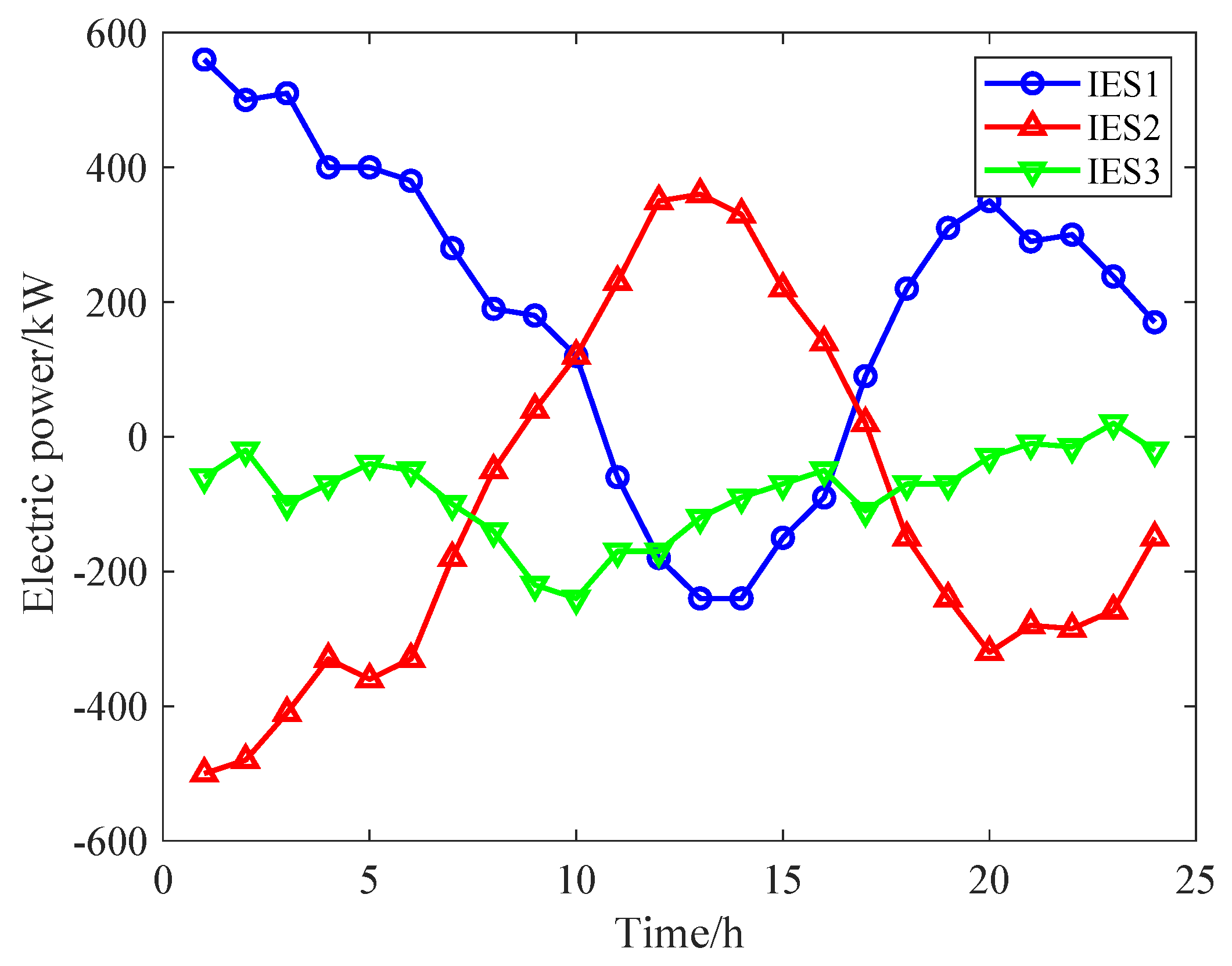
The proposed energy trading strategy requires determining the trading volumes and prices among IESs. The electrical and heat energy trading among the IESs are shown in Figure 6 and Figure 7.

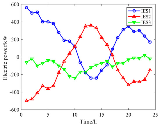
Figure 6. Electrical energy trading among IESs.

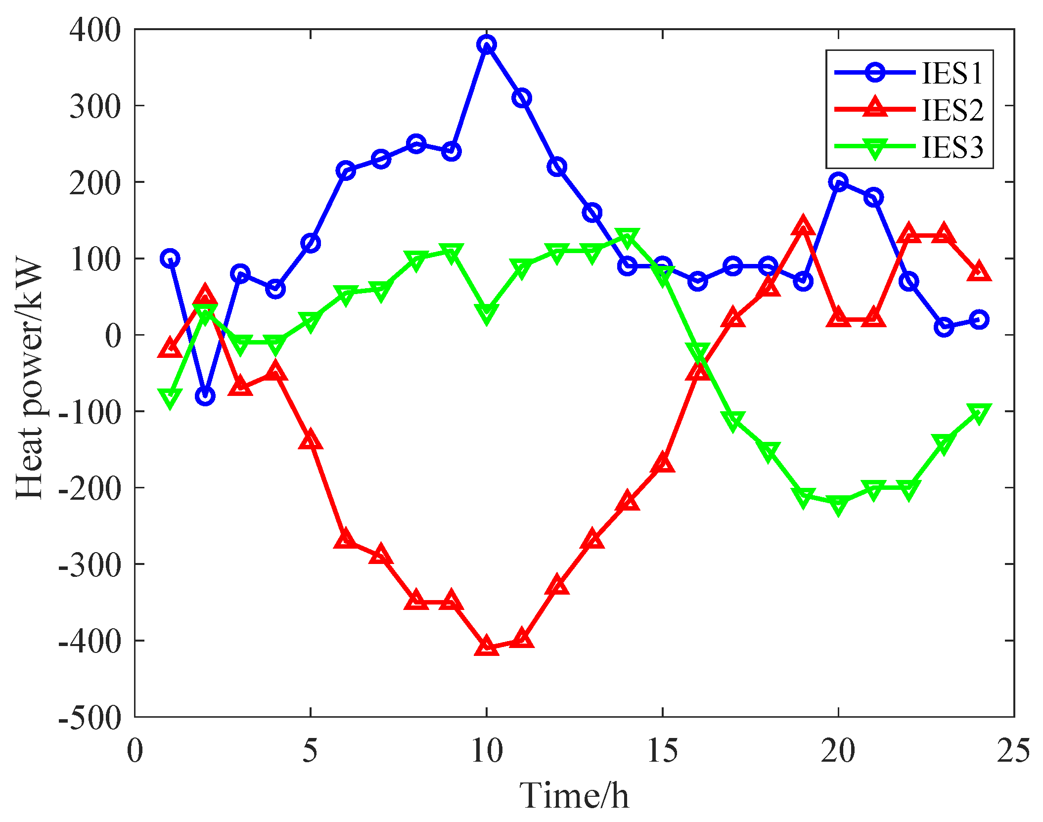
Figure 7. Heat energy trading among IESs.

From Figure 6, it can be observed that during the periods of t = 00:00–08:00 and 18:00–23:00, when PV generation is absent, IES2 faces a shortage of electrical energy. During these periods, IES1, with sufficient WT energy, supplies electricity to IES2. Conversely, during the period of t = 09:00–17:00, IES2’s PV power output exceeds its demand, leading IES2 to sell surplus electricity to IES1. From Figure 7, it can be observed that during the period of t = 03:00–18:00, IES2 experiences high load demand. Hence, IES2 purchases heat energy from IES1 and IES3 to meet the load requirements. In summary, the three distinct IESs actively engage in electrical and heat energy trading, achieving multi-energy complementarity and reducing their operating costs.

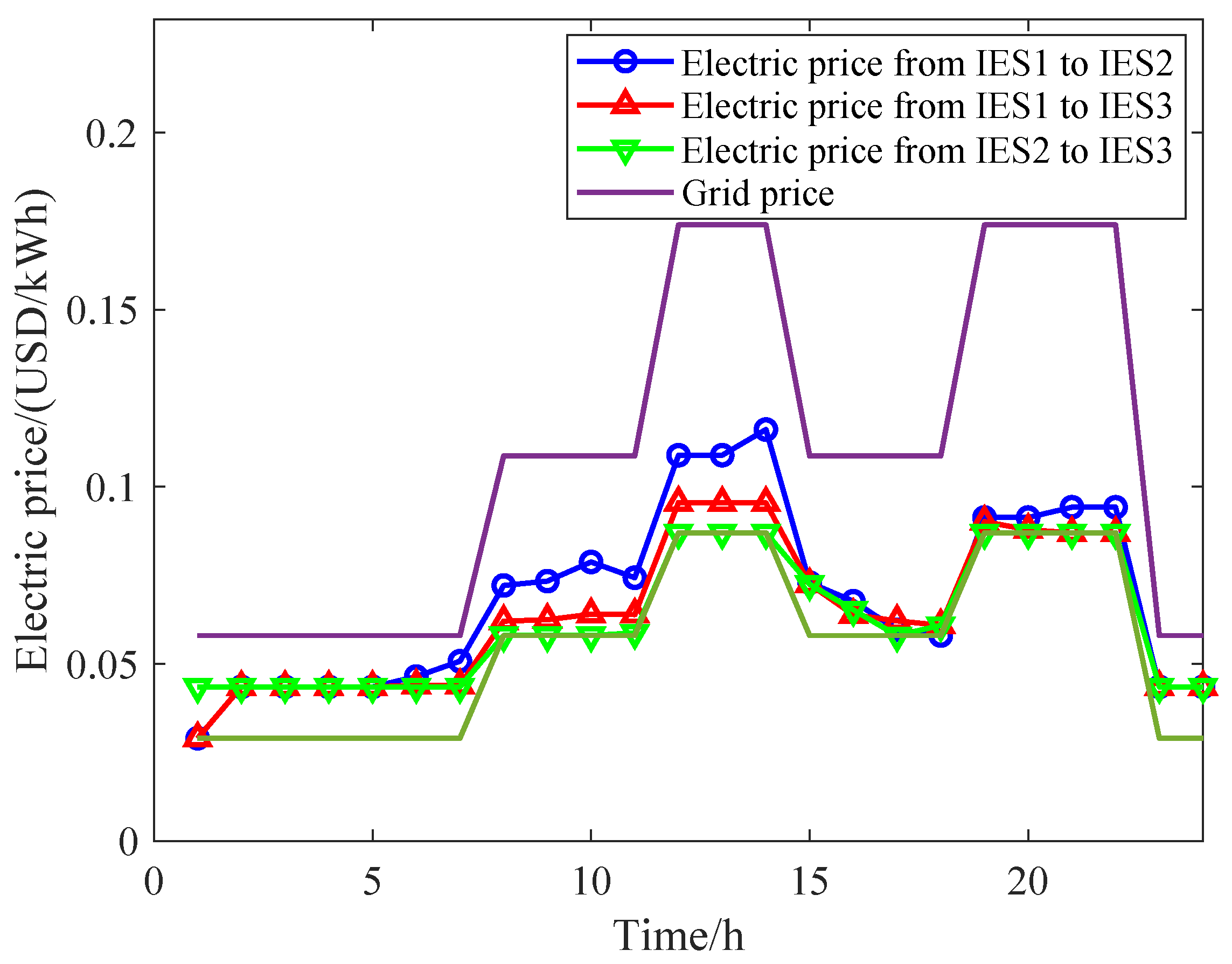
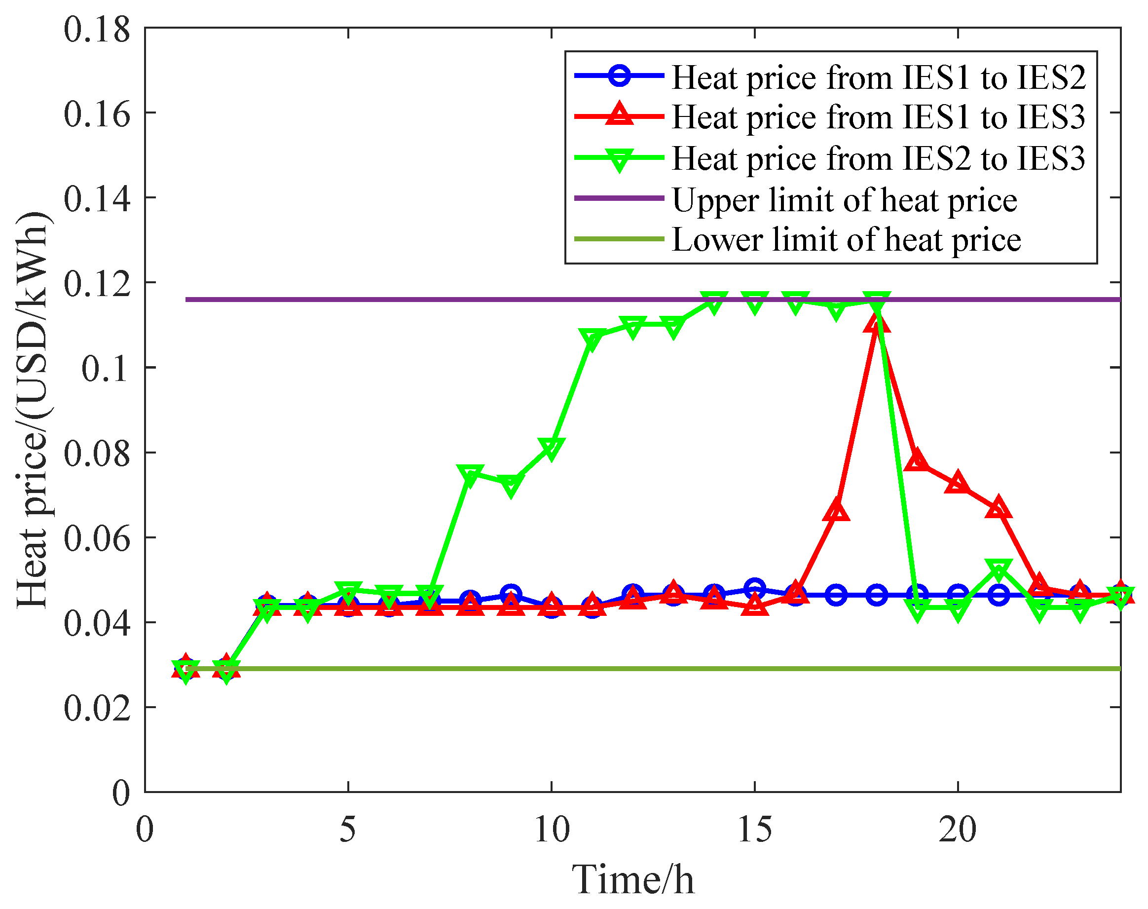
The negotiated prices of electrical and heat energies for each IESs are presented in Figure 8 and Figure 9. As shown in Figure 8, the optimal transaction prices are determined through Nash–Harsanyi, with electrical energy prices falling between the grid’s purchasing and selling prices. This allows the IESs to sell electrical energy to other IESs at higher purchasing prices than that of the grid and to buy electrical energy from other IESs at lower selling prices than that of the grid, effectively reducing operational costs. Similarly, Figure 9 shows that the heat energy transaction prices also fall into the upper and lower limits.

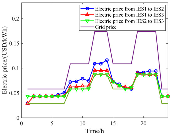
Figure 8. The price of electrical energy trading after Nash–Harsanyi.

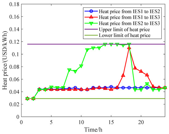
Figure 9. The price of heat energy trading after Nash–Harsanyi.

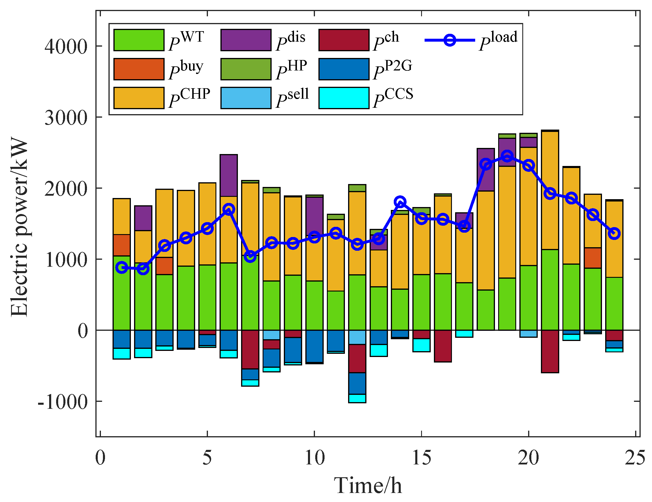
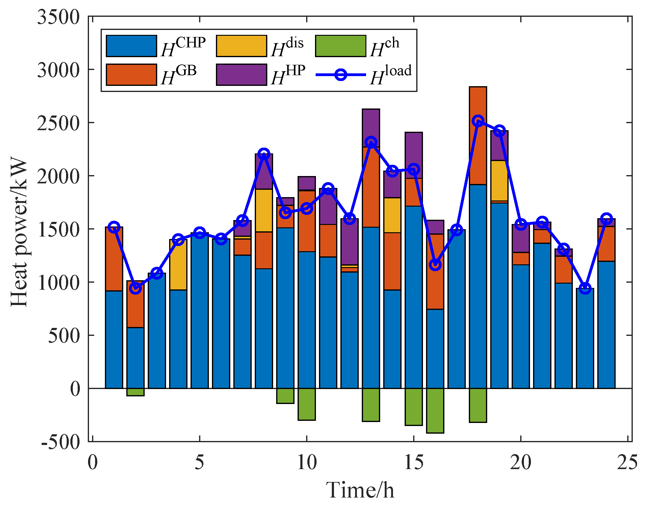
Figure 10 and Figure 11 present the optimized energy balance results for IES1. Regarding the electrical energy balance, IES1 reduces its electricity purchases and increases the CHP generation during the high electric price period. The electrical energy storage is primarily charged during t = 07:00–09:00 and discharged during t = 17:00–20:00. Regarding the heat energy balance, it is mainly generated by CHP, GB. The output of HP and heat energy storage is reduced to lower operating costs. Other IESs exhibit similar results and are not described in detail here.

Figure 10. The electrical energy balance of IES1.

Figure 11. The heat energy balance of IES1.

5.4. Benefit and Cost Analysis

Table 3 illustrates that the proposed method can improve benefits for all subjects involved and distribute them reasonably. Table 4 shows that the distribution of benefits varies with different methods. The Nash bargaining method aims to balance profit distribution based on equal contributions from each subject, but this is difficult to fully achieve in practice. The Shapley value method focuses solely on the marginal contributions of operators, without sufficiently considering other influencing factors. In contrast, the method proposed in this paper integrates multiple factors to achieve an equitable distribution of benefits, thereby promoting energy trading among the participants.

Table 3. The distribution of the benefits of the proposed method.

IES Number	IES1	IES2	IES3
Cost before cooperation/USD	2630.1	3912.5	2880.3
Final cost/USD	2174.2	3593.4	2495.1
Increase value/USD	455.9	319.1	385.2

Table 4. Comparison of benefits of different methods.

Methods	IESs Number	Revenue/USD	Increased Percentage
Nash solution	IES1	303.1	33.2%
	IES2	305.2	33.4%
	IES3	303.9	33.3%
Shapley value method	IES1	478.2	41.7%
	IES2	273.5	23.9%
	IES3	394.1	34.4%
Method of this paper	IES1	455.9	39.3%
	IES2	319.1	27.5%
	IES3	385.2	33.2%

5.5. Uncertainty Analysis

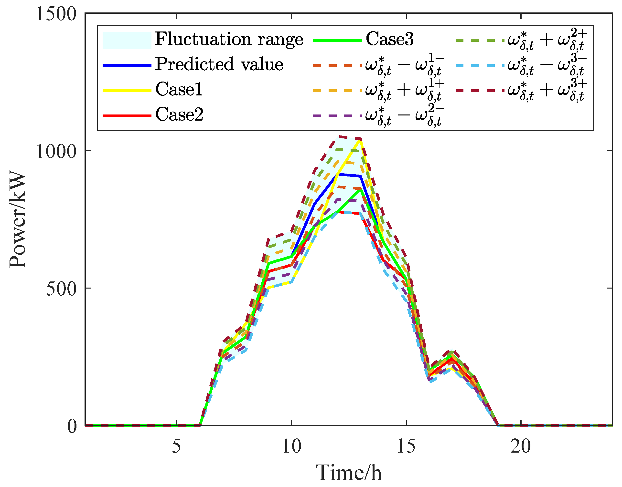
To evaluate the effectiveness of the proposed uncertainty method, a comparison of the following three cases is conducted:

Case 1: Traditional two-stage RO model with the uncertainty set shown in (11).

Case 2: Four-level RO model without considering balance, which is proposed in [21].

Case 3: Four-level RO model considering balance, which is proposed in this paper.

Figure 12 and Figure 13 present the optimization results of WT and PV for IES1 and IES2 under the three cases, respectively. In Case 1, the WT and PV output is observed to be located at the boundaries of the interval, indicating that the optimization result under this case is the most conservative. In Case 2, the conservatism of optimization results is reduced, but due to the lack of consideration for balance, the uncertainty decisions always occur in either downward or upward trend situations. In contrast, the optimization results in Case 3 can be distributed more evenly across all intervals, resulting in the lowest level of conservatism. Overall, by constructing uncertainty sets through dividing multiple intervals, scenarios with low probability can be reduced to better approximate actual conditions, thus aligning more closely with reality.

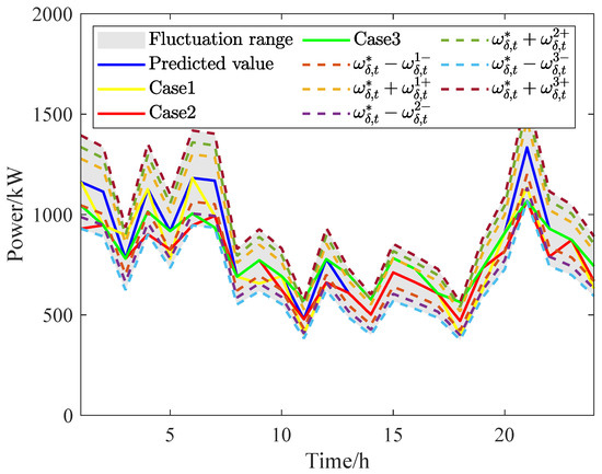
Figure 12. The optimization results of WT under different cases.

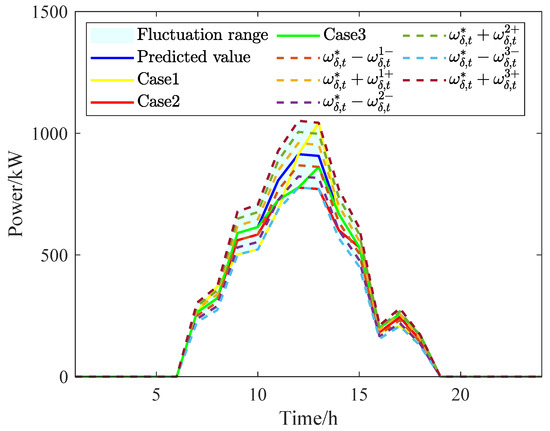
Figure 13. The optimization results of PV under different cases.

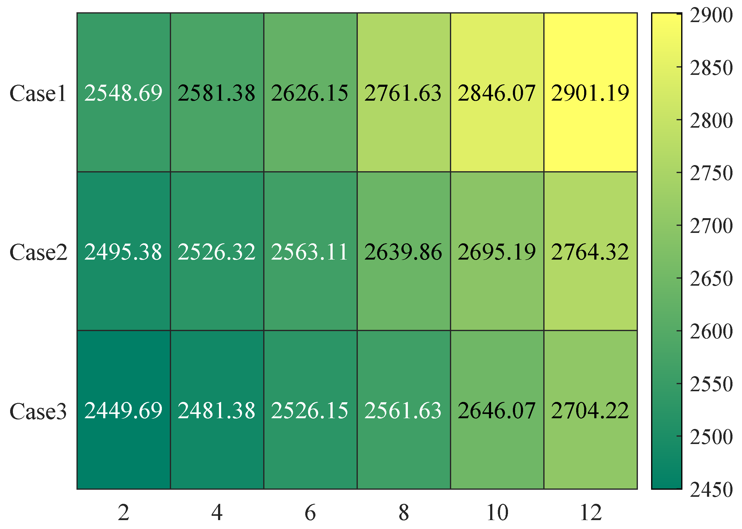
As shown in Figure 14, taking WT as an example, the operational costs of IES1 under different cases with uncertainty budgets are compared. When the uncertainty budget is set to 12, the total costs are 2901.19 USD for Case 1, 2764.32 USD for Case 2, and 2704.22 USD for Case 3, respectively. Among them, Case 3 achieves the lowest cost under the same uncertainty budget. Additionally, as the uncertainty budget increases, the model’s uncertainty gradually increases, leading to higher operational costs for the IES. Therefore, IES operators can set an appropriate uncertainty budget to adjust their operational strategy.

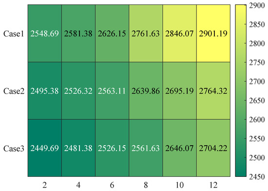
Figure 14. The optimization results of costs under different cases.

In addition, the comparison of the speed of different algorithms in solving the four-level robust model of IES1 is shown in Table 5. When directly applying the C&CG algorithm, the four-level robust model can be converted to a min-max-min model, but because the four-level robust model’s subproblem is nonlinear, Baron is used to solve it. According to Table 5, when Baron is used with the Gap set to zero, it fails to obtain the best solution in a reasonable time. When using the default gap setting, the solution time is 4351.19 s, with a cost of 2618.8 USD. However, when using the C&CG-AIS algorithm, it takes just 56.38 s. The C&CG-AIS algorithm further divides the original subproblem into two subproblems, greatly improving the solution’s efficiency.

Table 5. Comparison of different methods.

	C&CG (Gap = 0)	C&CG (Default Gap)	C&CG-AIS
Solver	Baron	Baron	Gurobi
Solving time/s	—	4351.19	56.38
Cost/USD	—	2618.8	2630.1
Outer/inner loop iterations	—	3/—	3/(2;3;2)

6. Conclusions

This paper presents an energy trading strategy for IESs. Firstly, a model incorporating P2G and CCS technologies is established to facilitate the low-carbon operation of the system. Secondly, a four-level robust optimization model is developed to reduce the impact of renewable energy uncertainty. To address the issue of benefit allocation among multiple IESs, the Nash–Harsanyi approach is used and decomposes the original problem into two subproblems. In P2, the bargaining power of each IES is quantified using marginal contribution and energy contribution, enabling a fair allocation of benefits. Finally, the model is solved using the ADMM algorithm to achieve fast convergence.

It is worth noting that the impact of changes in socio-economics, load, market electricity prices, and environmental competition also have a significant impact on energy trading. Additionally, IESs involve not only electrical and heat energies but also other forms of energy, such as hydrogen. These factors will be comprehensively considered in future research to develop more stable energy trading strategies.

References

- Yang, H.; Chu, Y.; Ma, Y.; Zhang, D. Operation strategy and optimization configuration of hybrid energy storage system for enhancing cycle life. J. Energy Storage 2024, 95, 112560. [Google Scholar] [CrossRef]
- Liu, S.; Shen, J.; Zhang, J. A novel configuration optimization approach for IES considering exergy-degradation and non-energy costs of equipment. Energy 2024, 312, 133600. [Google Scholar] [CrossRef]
- Chu, X.; Fu, L.; Liu, Q.; Yu, S. Optimal allocation method of oxygen enriched combustion-carbon capture low-carbon integrated energy system considering uncertainty of carbon-source-load. Int. J. Electr. Power Energy Syst. 2024, 162, 110220. [Google Scholar] [CrossRef]
- Ghafoor, A.; Aldahmashi, J.; Apsley, J.; Djurović, S.; Ma, X.; Benbouzid, M. Intelligent Integration of Renewable Energy Resources Review: Generation and Grid Level Opportunities and Challenges. Energies 2024, 17, 4399. [Google Scholar] [CrossRef]
- Wu, X.; Yang, L.; Zheng, B. Joint capacity configuration and demand response optimization of integrated energy system considering economic and dynamic control performance. Energy 2024, 301, 131723. [Google Scholar] [CrossRef]
- Ren, X.Y.; Li, L.L. Optimization and performance analysis of integrated energy systems considering hybrid electro-thermal energy storage. Energy 2024, 2024, 134172. [Google Scholar] [CrossRef]
- Wu, M.; Wu, Z.; Shi, Z. Low carbon economic dispatch of integrated energy systems considering utilization of hydrogen and oxygen energy. Int. J. Electr. Power Energy Syst. 2024, 158, 109923. [Google Scholar] [CrossRef]
- Dou, J.; Wang, X.; Liu, Z.; Sun, Q.; Wang, X.; He, J. Towards Pareto-optimal energy management in integrated energy systems: A multi-agent and multi-objective deep reinforcement learning approach. Int. J. Electr. Power Energy Syst. 2024, 159, 110022. [Google Scholar] [CrossRef]
- Li, J.; Wu, Y.; Ma, S.; Zhang, J.; Sun, X. Multi-objective optimization scheduling of integrated energy systems considering regional time-of-use electricity prices and weight sensitivity. Electr. Power Syst. Res. 2024, 236, 110905. [Google Scholar] [CrossRef]
- Zhou, C.; Zheng, C.B. Energy Trading Strategy for Heat and Electricity-Coupled Microgrid Based on Cooperative Game. Appl. Sci. 2022, 12, 6568. [Google Scholar] [CrossRef]
- Chen, J.; Tang, Z.; Huang, Y.; Qiao, A.; Liu, J. Asymmetric Nash bargaining-based cooperative energy trading of multi-park integrated energy system under carbon trading mechanism. Electr. Power Syst. Res. 2024, 228, 110033. [Google Scholar] [CrossRef]
- Zhang, Y.; Wu, Q.; Ren, H.; Li, Q.; Zhou, W. A multi-agent distributed electricity-carbon shared trading strategy considering regional carbon inclusion. Renew. Energy 2024, 239, 122075. [Google Scholar] [CrossRef]
- Chen, W.; Wang, J.; Yu, G.; Chen, J.; Hu, Y. Research on day-ahead transactions between multi-microgrid based on cooperative game model. Appl. Energy 2022, 316, 119106. [Google Scholar] [CrossRef]
- Xu, D.; Zhou, B.; Liu, N.; Wu, Q.; Voropai, N.; Li, C.; Barakhtenko, E. Peer-to-peer multienergy and communication resource trading for interconnected microgrids. IEEE Trans. Ind. Inform. 2020, 17, 2522–2533. [Google Scholar] [CrossRef]
- Wang, L.; Zhang, Y.; Song, W.; Li, Q. Stochastic cooperative bidding strategy for multiple microgrids with peer-to-peer energy trading. IEEE Trans. Ind. Inform. 2021, 18, 1447–1457. [Google Scholar] [CrossRef]
- Singh, K.; Gadh, R.; Singh, A.; Dewangan, C.L. Design of an optimal P2P energy trading market model using bilevel stochastic optimization. Appl. Energy 2022, 328, 120193. [Google Scholar] [CrossRef]
- Khan, S.S.; Ahmad, S.; Naeem, M. On-grid joint energy management and trading in uncertain environment. Appl. Energy 2023, 330, 120318. [Google Scholar] [CrossRef]
- Gao, J.; Shao, Z.; Chen, F.; Chen, Y.; Lin, Y.; Deng, H. Distributed robust operation strategy of multi-microgrid based on peer-to-peer multi-energy trading. Iet Energy Syst. Integr. 2023, 5, 376–392. [Google Scholar] [CrossRef]
- Siqin, Z.; Niu, D.; Wang, X.; Zhen, H.; Li, M.; Wang, J. A two-stage distributionally robust optimization model for P2G-CCHP microgrid considering uncertainty and carbon emission. Energy 2022, 260, 124796. [Google Scholar] [CrossRef]
- Wang, S.; Wang, S.; Zhao, Q.; Dong, S.; Li, H. Optimal dispatch of integrated energy station considering carbon capture and hydrogen demand. Energy 2023, 269, 126981. [Google Scholar] [CrossRef]
- Zhong, J.; Li, Y.; Cao, Y.; Tan, Y.; Peng, Y.; Zhou, Y.; Nakanishi, Y.; Li, Z. Robust coordinated optimization with adaptive uncertainty set for a multi-energy microgrid. IEEE Trans. Sustain. Energy 2022, 14, 111–124. [Google Scholar] [CrossRef]
- Gao, J.; Shao, Z.; Chen, F.; Lak, M. Robust optimization for integrated energy systems based on multi-energy trading. Energy 2024, 308, 132302. [Google Scholar] [CrossRef]
Disclaimer/Publisher’s Note: The statements, opinions and data contained in all publications are solely those of the individual author(s) and contributor(s) and not of MDPI and/or the editor(s). MDPI and/or the editor(s) disclaim responsibility for any injury to people or property resulting from any ideas, methods, instructions or products referred to in the content. |
© 2025 by the authors. Licensee MDPI, Basel, Switzerland. This article is an open access article distributed under the terms and conditions of the Creative Commons Attribution (CC BY) license (https://creativecommons.org/licenses/by/4.0/).