Forecasting Heat Power Demand in Retrofitted Residential Buildings

Abstract

The accurate prediction of heat demand in retrofitted residential buildings is crucial for optimizing energy consumption, minimizing unnecessary losses, and ensuring the efficient operation of heating systems, thereby contributing to significant energy savings and sustainability. Within the framework of this article, the dependence of the energy consumption of a thermo-modernized building on a chosen set of climatic factors has been meticulously analyzed. Polynomial fitting functions were derived to describe these dependencies. Subsequent analyses focused on predicting heating demand using artificial neural networks (ANN) were adopted by incorporating a comprehensive set of climatic data such as outdoor temperature; humidity and enthalpy of outdoor air; wind speed, gusts, and direction; direct, diffuse, and total radiation; the amount of precipitation, the height of the boundary layer, and weather forecasts up to 6 h ahead. Two types of networks were analyzed: with and without temperature forecast. The study highlights the strong influence of outdoor air temperature and enthalpy on heating energy demand, effectively modeled by third-degree polynomial functions with R² values of 0.7443 and 0.6711. Insolation (0–800 W/m²) and wind speeds (0–40 km/h) significantly impact energy demand, while wind direction is statistically insignificant. ANN demonstrates high accuracy in predicting heat demand for retrofitted buildings, with R² values of 0.8967 (without temperature forecasts) and 0.8968 (with forecasts), indicating minimal performance gain from the forecasted data. Sensitivity analysis reveals outdoor temperature, solar radiation, and enthalpy of outdoor air as critical inputs.

1. Introduction

Shaping the modern housing environment should occur under the conditions of sustainable development [1]. According to the hierarchy of basic human needs, after satisfying essential physiological requirements, we aim to secure adequate safety, housing, and energy production [2].

The authors of this article seek to identify the relationships among various factors influencing energy demand in modernized buildings, ultimately developing an algorithm to determine the required amount of thermal energy drawn from district heating networks. The research scope was defined according to technical criteria reflecting sustainable urban development (SUD) [3]. Consequently, managing Demand-Side Management (DSM) in urban areas becomes vital in the context of future SUD and a climate-neutral energy economy [4,5].

Predicting energy demand has been an important field of research for many years. These processes use complex algorithms, also using artificial neural networks (ANNs) to develop a model of effective energy consumption. Thanks to new computational technologies using multiple ANN models, the results become more precise and more effective in the implementation process [6].

Climatic conditions, such as insolation, wind speed and direction, temperature, and humidity, have a significant impact on the heat demand of buildings both before and after thermal upgrading. Retrofitting, which includes increasing wall insulation and replacing windows, changes the way a building responds to these factors. Increasing wall insulation reduces heat loss by infiltration, which reduces heating demand during colder periods. However, better insulation can reduce passive solar heat gain, as less solar energy penetrates a well-insulated envelope. As a result, additional heating may be needed during transitional periods to maintain thermal comfort [7]. Outdoor air temperature and humidity affect heat loss through the envelope and the efficiency of heating and ventilation systems. Thermal retrofitting improves the thermal insulation of a building, which reduces the impact of varying outdoor conditions on indoor comfort [8].

2. Advanced Method of Energy Consumption Assessment in Buildings

Aligning building energy requirements with the principles of sustainable urban development (SUD) necessitates the adoption of appropriate technologies by users, managers, and designers. Reducing carbon emissions while optimizing household energy consumption in residential buildings has emerged as a global imperative.

The application of energy demand management, particularly in retrofitted buildings, involves a complex interplay of socio-economic and technical factors. Within the framework of Demand-Side Management (DSM), these measures aim to achieve tangible energy savings, thereby improving living conditions while supporting SUD objectives [9].

A gradual and systematic approach to implementing energy optimization is a policy goal for many countries. For example, in China, long-term economic planning and legislative provisions focus on introducing new technologies, monitoring implementation, and achieving measurable energy savings [10].

However, optimizing energy use in buildings is not solely about improving economic efficiency. Equally significant is the need to manage energy flow, enhance data integration, and enable sustainable forecasting. These efforts support intelligent, controlled energy consumption tailored to various building types. Studies evaluating building energy consumption often emphasize savings achieved through energy distribution and management processes. This issue is particularly relevant in countries with shorter heating seasons, such as those in Southern Europe, where energy use aligns with scheduled delivery periods. These actions have demonstrated significant reductions in primary energy consumption—66%, 74%, and 65% in continuously heated residential buildings in Greece, Portugal, and Spain, respectively [11].

The non-energy benefits of retrofitting are frequently overlooked. Beyond reducing carbon footprints, retrofits can lower the atmospheric emissions of greenhouse gases, such as SOx, NOx, and benzopyrene. Complex retrofitting processes, often referred to as deep thermo-modernization, have shown variable success in improving energy and environmental performance. For instance, results indicate that deep retrofitting benefits educational buildings not in all conditions. Without financial subsidies, the complexity and cost of these processes may render them unfeasible [12].

The global trend of constructing energy-efficient buildings necessitates constant comparison with reference buildings of similar types to evaluate the achieved energy outcomes. Combining home control systems with energy-saving measures can enhance energy efficiency by reducing demand and improving monitoring and management processes—especially in smart technologies [13,14].

The search for the relationship between the economic efficiency of the thermo-modernization solutions used in relation to the energy effects achieved has become the primary determinant of the implementation of appropriate technical solutions. In many cases, it is easier to apply costly technologies with the use of renewable energy sources in public utility buildings, such as educational, administrative, or health care facilities, due to the participation and involvement of public and private capital in the processes [15].

The growing demand for energy efficiency in buildings has led to the development of advanced artificial intelligence (AI) techniques for predicting heat power demand, especially in heating, ventilation, and air conditioning (HVAC) systems. The adoption of advanced technologies, such as artificial neural networks (ANNs), has shifted from being a challenge to becoming a necessity. ANNs provide an alternative method for solving complex problems by learning from historical data rather than traditional programming techniques [16].

It turns out that ongoing research [17] in this area must distinguish between energy demand and energy consumption forecasting, which, given the vast amount of output data, should be conducted using ANNs. Therefore, it was crucial to examine how ANNs were implemented and on which models. Additionally, the results achieved with these models and the emerging trends were assessed. Understanding these principles aimed to eliminate the increasingly common phenomena of repetitive applications and methods used in developing action models to optimize the performance of machine learning (ML) techniques.

Predictive systems use data on atmospheric conditions (e.g., outdoor temperature, insolation, and wind speed), building characteristics, and occupancy patterns. On this basis, it is possible to forecast variable thermal energy demand. For example, during periods of intense sunshine, the control system can reduce heating to take advantage of natural heat gains, while during periods of high winds, it takes into account additional losses through ventilation or thermal bridges. The prediction of heat demand in thermally upgraded buildings is crucial to fully realize the potential of energy efficiency. By accurately predicting energy demand, it is possible to implement intelligent control systems that dynamically adjust heat supply to the actual needs of the building, minimizing energy losses.

The process of modeling and forecasting energy consumption in multi-family residential buildings still appears to be underdeveloped. Such research can yield reliable and simultaneously optimal solutions for creating energy consumption simulations. Computational models based on the Levenberg–Marquardt and OWO–Newton algorithms achieved noteworthy determination coefficients in the range of 0.87–0.91, which is a strong result and comparable to findings reported in other publications [18].

The work and analyses aimed at finding appropriate methods and algorithms for forecasting energy consumption in residential buildings based on ANNs must be continuously corrected and improved. Energy consumption and the prediction of hourly load profiles enabled the evaluation of variable relevance as well as the determination of the number of free parameters required to construct the output model [19]. The obtained results demonstrated that statistical analysis, as a significant component of neural models, can serve as a valuable tool for developing simple and, most importantly, highly efficient neural models specifically applicable in the field of building energy management.

One of the methods to optimize the results obtained is their multi-source extraction and comparison. Another study [20] used three new methods of intelligent grasshopper optimization algorithm (GOA), wind-driven optimization (WDO), and biogeography-based optimization (BBO), which influenced the optimized prediction of heating loads and cooling loads of buildings.

The necessary factors to consider in forecasting energy consumption (including electricity) took into account demand and ambient temperature from the perspective of hourly or seasonal variation. This makes it difficult to match energy consumption during periods of long-term and short-term demand in the same time frame. Another study on office buildings was to compare the forecasting results obtained by the traditional method and the ANN method [21]. The proposed approach divides energy demand data into fixed time periods that include operating hours to reduce the impact of human activity. Once a suitable weather variable is found to match the energy demand during working hours, the building’s energy constant can be predicted here. The second proposed approach uses an ANN to match hourly load, peak load, and occupancy rate with multiple variables. In this approach, data for energy demand is divided into shorter time ranges, hours with no occupancy, hours of full occupancy, and fuzzy hours in between, where occupancy rates vary with time and weather variables. The proposed approaches are validated by case study data. Simulation results show, comparing the traditional method with the ANN method, that both proposed approaches have less root-mean-square error (RMSE) in predicting building electricity demand.

In another article [22], researchers compare the prediction capabilities of five different intelligent system techniques for predicting electricity consumption in administrative buildings in the UK. These five techniques are multiple regression (MR), genetic programming (GP), artificial neural network (ANN), deep neural network (DNN), and support vector machine (SVM). The models are developed based on five years of observed data of five different output parameters, such as solar radiation, temperature, wind speed, humidity, and weekday index. The weekday index is an important parameter for distinguishing between working days and days off. The results show that ANN performs better than all the other four techniques with a percentage error (MAPE) of 6%, while MR, GP, SVM, and DNN have 8.5%, 8.7%, 9%, and 11%, respectively. The authors also emphasize that this type of research can also cover other categories of buildings and will help optimize energy consumption forecasting for different types of buildings in the future.

A recent study from 2024 using ANNs is the reverse of the previous post [23]. All scholars have used a bottom-up model, i.e., extensive simulations and calculations of energy consumption of buildings, but here we are dealing with a model for predicting hourly heat demand at the national level. This approach significantly reduces the time and complexity of the prediction by reducing the number of model input types through feature selection (making the model more realistic). Such a model can be adapted using less meteorological data, while accurately predicting hourly heat demand throughout the year. The model provides a framework for obtaining accurate heat demand forecasts for large-scale areas, which in turn can be used as a reference for making appropriate decisions.

Another study [24] in this area addresses the issues of using ANN to predict the heat demand associated with air conditioning in non-residential buildings. The reliable preliminary prediction of the thermal energy demand of a building is performed with the help of detailed dynamic simulation software, which also requires knowledge of the heat balance and several output data. The authors’ research goal was to identify the best ANN topology, developing a tool for determining both fast and simple thermal energy demand of a non-residential building with only 12 well-known thermophysical parameters without using thermal balance data. The authors describe how to train a network to develop an accurate thermal energy database to form the basis of specific ANNs. Another approach to the study involves considering an ensemble of neural networks [25]. Various ANNs are used to predict thermal energy consumption on a university campus: forward neural network (FFNN), radial basis function network (RBFN), and adaptive neuro-fuzzy interference system (ANFIS). For each type of neural network, three models are analyzed (using different initial parameters). In order to achieve accuracy in predicting energy consumption, not just individual networks but the entire ensemble of neural networks is studied. Three different combinations of results are then analyzed. The study shows that all the proposed neural networks can predict heat consumption with high accuracy. Using the whole ensemble of networks gives even more precise results. ANN, due to their capacity for capturing complex, nonlinear relationships between various factors like weather conditions and occupancy rates, have shown substantial promise in reducing prediction errors [26]. Moreover, multi-objective optimization methods, such as those employing the Artificial Bee Colony (ABC) algorithm, effectively balance energy efficiency with indoor thermal comfort [27].

Research also emphasizes the application of artificial intelligence in district heating systems, where machine learning models and ensemble techniques improve the accuracy of heat demand forecasts [28,29]. Unsupervised learning algorithms, such as K-means clustering, have been applied to enhance the performance of HVAC systems by creating zone-specific heating management strategies [30]. Additionally, advanced pre-processing techniques like wavelet transforms, coupled with tree-based ensemble models, further improve forecasting accuracy by accounting for temporal variability in heating loads [31]. Collectively, these AI-driven approaches contribute to enhanced energy management, lower operational costs, and better thermal comfort in buildings.

In this study, we classified ANN into two distinct groups: those incorporating temperature forecasts several hours ahead and those operating without temperature forecasts. This methodological division represents a novel contribution to the field, addressing a significant gap in the existing research. Few scientific studies have conducted such comparative analyses in the context of predicting heat demand for buildings, particularly after thermal retrofitting—a critical area of investigation as retrofitting significantly alters thermal dynamics. By comparing these two network types, we aim to elucidate the role of outdoor temperature forecasts in enhancing model accuracy and robustness, offering deeper insights into their relative advantages and limitations. The integration of outdoor temperature forecasts accounts for future climatic variability, potentially improving demand prediction precision. Conversely, networks without forecasts represent a more generalized approach, applicable where forecast data are unavailable or unreliable. This comparison provides a comprehensive framework for optimizing ANN applications in real-world energy management scenarios, setting a precedent for future research.

3. Materials and Methods

3.1. General Description

Within the scope of this paper, the comparative results of the measured actual thermal energy demand for heating a multi-family residential building to the predicted thermal energy demand determined from general meteorological data are presented. Demand prediction was performed using ANN, and the following variables were used as input data: outdoor air temperature t_ext (°C), outdoor air enthalpy h_ext (kJ/kg), wind speed w_s (km/h), wind direction w_d (°), wind gust w_g (km/h), boundary layer height h_bl (m), direct radiation i_dir (W/m²), diffuse radiation i_dif (W/m²), total radiation i_tot (W/m²), and general information like month and hour.

Air enthalpy is the total energy content of air, comprising both sensible heat (due to its temperature) and latent heat (due to moisture content or phase changes in water vapor). The air boundary layer height is the vertical distance from the surface to the level where turbulent fluxes of momentum, heat, or mass diminish significantly, typically marking the transition from surface-driven turbulence to free atmospheric conditions. Direct radiation refers to solar radiation that travels in a straight line from the sun to a surface without being scattered, diffuse radiation is solar radiation that has been scattered by atmospheric particles and arrives at a surface from multiple directions, and total radiation is the sum of both direct and diffuse radiation received by a surface.

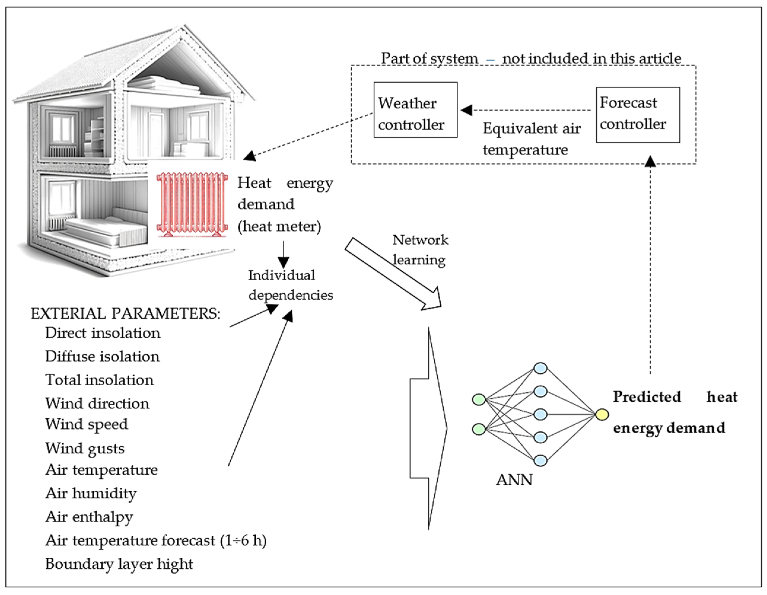
In addition, neural networks were also determined for which additional variables related to the predicted weather from the weather service were taken into account predicted temperature (°C) from 1 to 6 h ahead: t_+1h, t_+2h, t_+3h, t_+4h, t_+5h, t_+6h. A flowchart illustrating the conducted analysis is shown in Figure 1.

A correct estimation of the instantaneous heating energy demand allows for the optimal control of the heat or heat carrier supply. By taking all the meteorological factors into account, it is possible to make fuller use of heat gains or compensate for excessive heat losses. By knowing the dynamics of demand changes and the inertia of the heating system and the heated object, control can be intelligently implemented in advance.

In the beginning, the relationship between heating energy demand and individual climatic variables, including outdoor temperature, air enthalpy, total solar radiation, wind speed, and wind direction, was analyzed. Polynomial fitting functions were derived to model these dependencies. The statistical significance of the fitted models was evaluated using the ANOVA test, with results confirming significance at the 0.05 significance level. This analysis provides robust evidence of the influence of these climatic factors on energy demand, validating the relevance of the selected variables in energy modeling.

Subsequent analyses focused on predicting heating demand using ANN by incorporating a comprehensive set of climatic data. This approach aimed to leverage the full range of meteorological variables. By utilizing the available climate data, the ANN models were designed to capture complex interactions and nonlinear relationships between environmental factors and energy requirements, ensuring a more holistic and precise forecasting framework.

The prediction of energy demand for heating is, therefore, extremely important in terms of emulating the equivalent outdoor temperature. The heat demand can be determined according to the following formula:

$${\dot{Q}}_H=H·\left(t_i-t_e\right)$$

where ${\dot{Q}}_H$—heat energy flux (kW), H—building heat loss coefficient (W/K), t_i—design indoor temperature (°C), and t_e—outdoor temperature (°C). Thus, from the transformation of the modified formula,

$${\dot{Q}}_{H,pred}=H·\left(t_i-t_{e,eq}\right)$$

where ${\dot{Q}}_{H,pred}$—predicted heat energy flux (kW) and t_e,eq—equivalent outdoor temperature (°C), and the equivalent temperature can be determined as follows:

$$t_{e,eq}=t_i-{\displaystyle \frac{{\dot{Q}}_{pred}}{H}}$$

The equivalent outdoor temperature is emulated by the forecast controller for the weather control system.

It was decided to predict the heat demand since heat consumption is a directly measurable value. An approved heat meter that complies with the current technical requirements is used for the heat measurements. The predicted demand is very easy to compare to the current one. Another approach would be to directly determine the equivalent outdoor temperature based on climatic conditions, but verifying that value would be difficult.

In this research, the article does not present the results of the outdoor temperature t_ext,eq emulation but instead focuses on estimating thermal energy consumption under the given conditions.

3.2. Measurement System

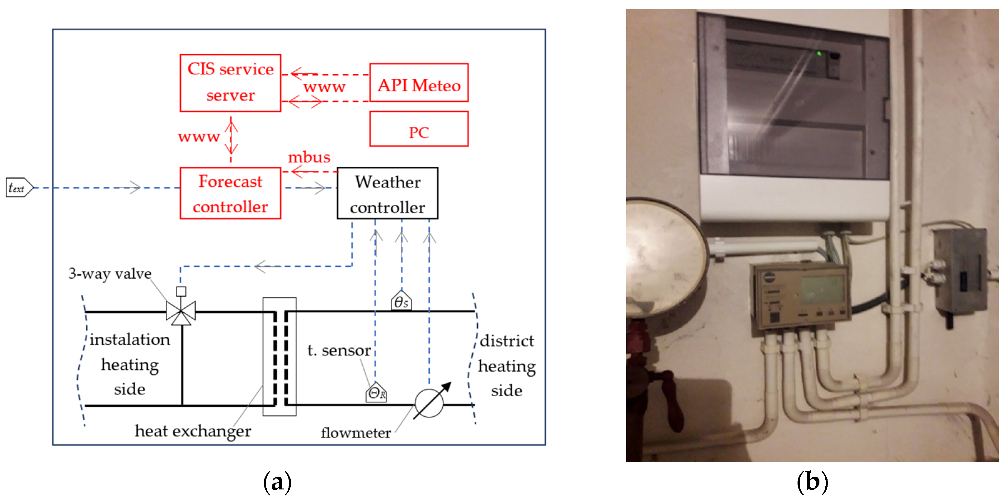
A typical control system for a heating system is weather control. Figure 2a shows a schematic diagram of the heat exchanger in the building, connected to the district heating network (elements marked in black). The exchanger is designed for the heating system, without a hot water heating circuit. The controller measures the outdoor temperature t_e and controls the supply temperature of the heating system through the three-way valve. From the measurement of the supply and return temperatures of the medium, as well as the mass flow, the consumed thermal energy (kW) is determined.

A modification in the system is a forecast controller connected via the Internet to the chief information system (CIS) server (polish acronym: NSI). This system is highlighted in red on the schema. The CIS additionally retrieves the current meteorological information from the API Meteo application for the geographic location specific to the installation site indicated in the settings. Then, the CIS determines the equivalent outdoor temperature. A data packet with the current external equivalent temperature settings for several hours ahead is sent hourly from the server to the forecast controller. The forecast controller emulates the outdoor temperature to the weather controller by adjusting the resistance value depending on the type of resistive outdoor temperature sensor. In addition, via the M-Bus interface, the forecast controller reads parameters from the weather controller that are related to thermal energy measurement and then sends them to the CIS. Measurements that were read by the forecast controller modules were outdoor temperature, supply temperature, return temperature, heating medium flow, delivered power, and heat consumption with an interval of every 10 min [32,33].

In weather mode, the forecast controller sends an unchanged temperature value to the weather controller, while in forecast mode, the equivalent temperature could be emulated depending on the estimated heat power demand Q_pred. The system works ideally with weather controllers in heat exchangers connected to the municipal heat network.

3.3. Characteristics of the Studied Building with Their Heating Systems

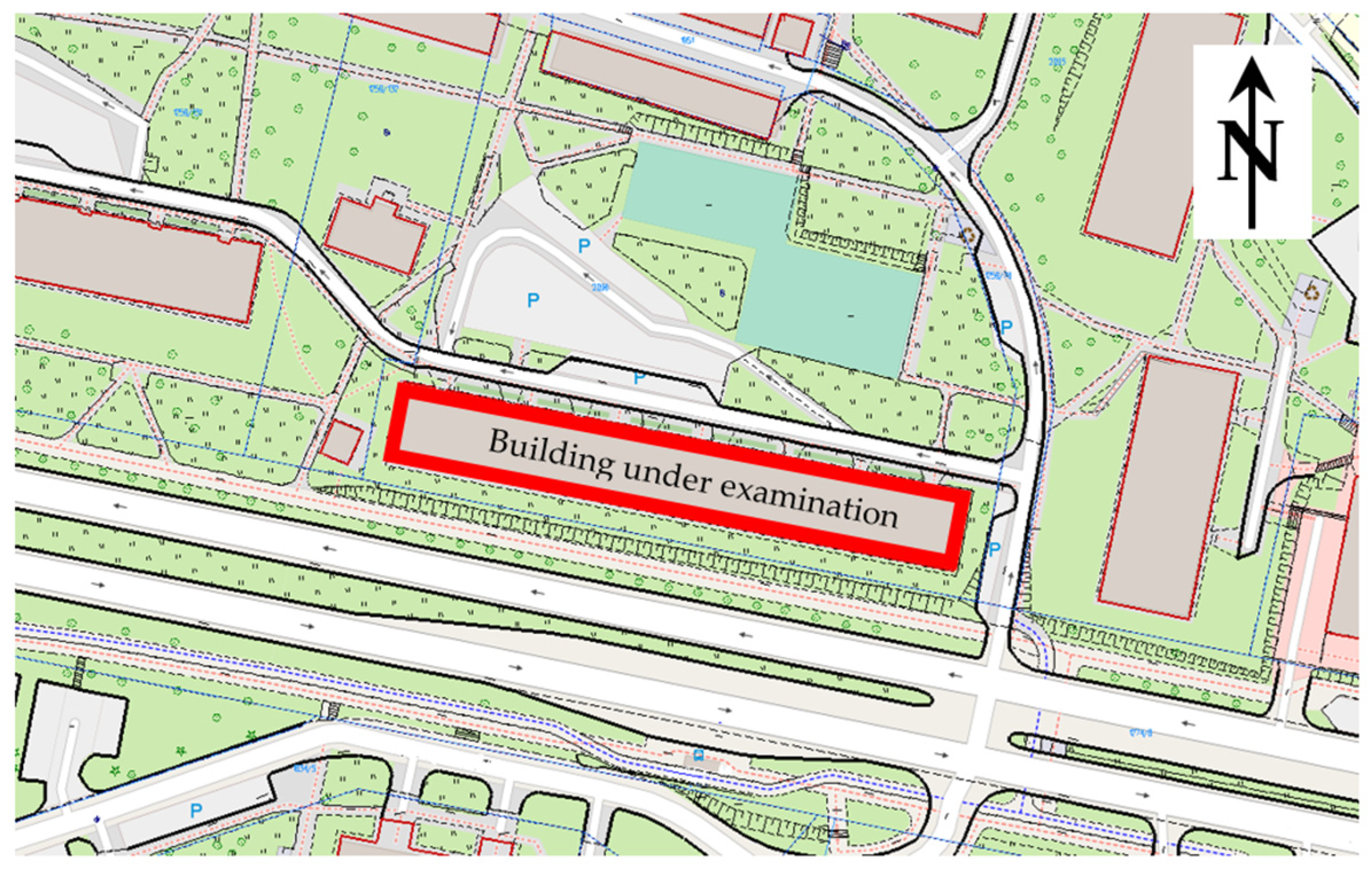
The subject of the study (Figure 3) was a multi-family building located in eastern Poland. The city is located in the III climatic zone, where the design temperature is −20 °C and the average outdoor temperature is +7.6 °C.

The object under study is a multi-family building built in the 1980s ÷ 1990s. The building is 5-story, with a basement, with a floor area of 5430 m² and a volume of 14,661 m³. The building is in an area of multi-family housing, while there are numerous wooded areas between the buildings. The estimated number of residents in 75 apartments is 225 residents. The average design indoor temperature is +20 °C.

The building underwent thermal modernization. The external walls were insulated with expanded polystyrene (EPS) and finished with a mineral plaster coating. The heating system is made in the traditional way as water heating, with convection heaters. Distribution pipes (bottom distribution) are installed in the basement, to which numerous risers are connected. Radiators connected to the risers are equipped with thermostatic valves. The building is supplied with thermal energy from the high-parameter municipal district heating network through a heat exchanger room located on the ground floor of the building.

Additionally, windows in the stairwells and the main entrance doors were replaced to improve energy efficiency. In residential units, windows were gradually replaced by unit owners during periodic renovations as needed. Minor improvements were also made to the heating system, including replacing the outdated heat exchanger room with modern plate heat exchangers, equipping the risers with automatic balancing valves, and insulating the basement piping. The ventilation system remained unchanged and continued to operate as a natural (gravitational) system.

3.4. Data for ANN Analysis

Measurement data covers the range from 26 January 2021 to 13 October 2024. Readings were exported from CIS to a comma-separated data text file (*.csv).

The software tool utilized for the analysis was Statistica TIBCO Software Inc., version 14.0.0.15, employing the automatic ANN module. Within this framework, feed-forward regression neural networks were constructed. Each network consisted of a single hidden layer, containing between 25 and 35 neurons. The maximum number of hidden neurons was determined based on the formula 2n + 1, where n represents the number of input variables. This limitation on the number of hidden neurons was intentionally applied to mitigate the risk of overfitting, thereby enhancing the network’s generalization ability.

For activation functions, a diverse range was employed, including identity, logistic, hyperbolic tangent (tanh), and exponential functions, applied to both the hidden and output neurons. The networks were configured with input features corresponding to either 11 variables (without temperature predictions) or 17 variables (with temperature predictions). The specific inputs included outdoor temperature (°C), exterior air enthalpy (kJ/kg), wind speed (km/h), wind direction (°), wind gust (km/h), boundary layer height (m), direct solar radiation (W/m²), diffuse solar radiation (W/m²), total solar radiation (W/m²), temperatures forecast for future intervals (t_+1h through t_+6h), and other qualitative variables as with month and hour.

Each network generated a single output, representing the predicted heat demand. The dataset used comprised 18,184 valid records, which were randomly divided into training (70%), testing (15%), and validation (15%) subsets.

We used MLP (multi-layer perceptron) neural network in the format “MLP X-Y-Z”, where X represents the number of input nodes, Y the hidden neurons, and Z the output node. The networks without temperature forecasts have 11 input nodes, reflecting the basic meteorological parameters, while those with temperature forecasts include 17 input nodes to account for the additional predictive temperature data. The networks utilize the BFGS (Broyden–Fletcher–Goldfarb–Shanno) training algorithm, a popular choice for optimization in neural networks due to its efficiency in handling nonlinear problems. The error function SOS (sum of squares) is uniformly applied across all the models, ensuring consistency in optimization.

A total of 100 neural networks were trained, and from these, the five models demonstrating the highest validation accuracy were selected for further analysis. This rigorous approach ensured a robust evaluation and optimized the models’ predictive performance while preserving their generalizability to new data.

4. Results

4.1. Summary of Meteorological Factor

The study, conducted over nearly four years, examined the impact of various climatic factors on thermal energy demand for building heating, focusing primarily on outdoor air temperature, along with wind parameters, external air enthalpy, and solar radiation.

4.1.1. Outdoor Temperature and Humidity

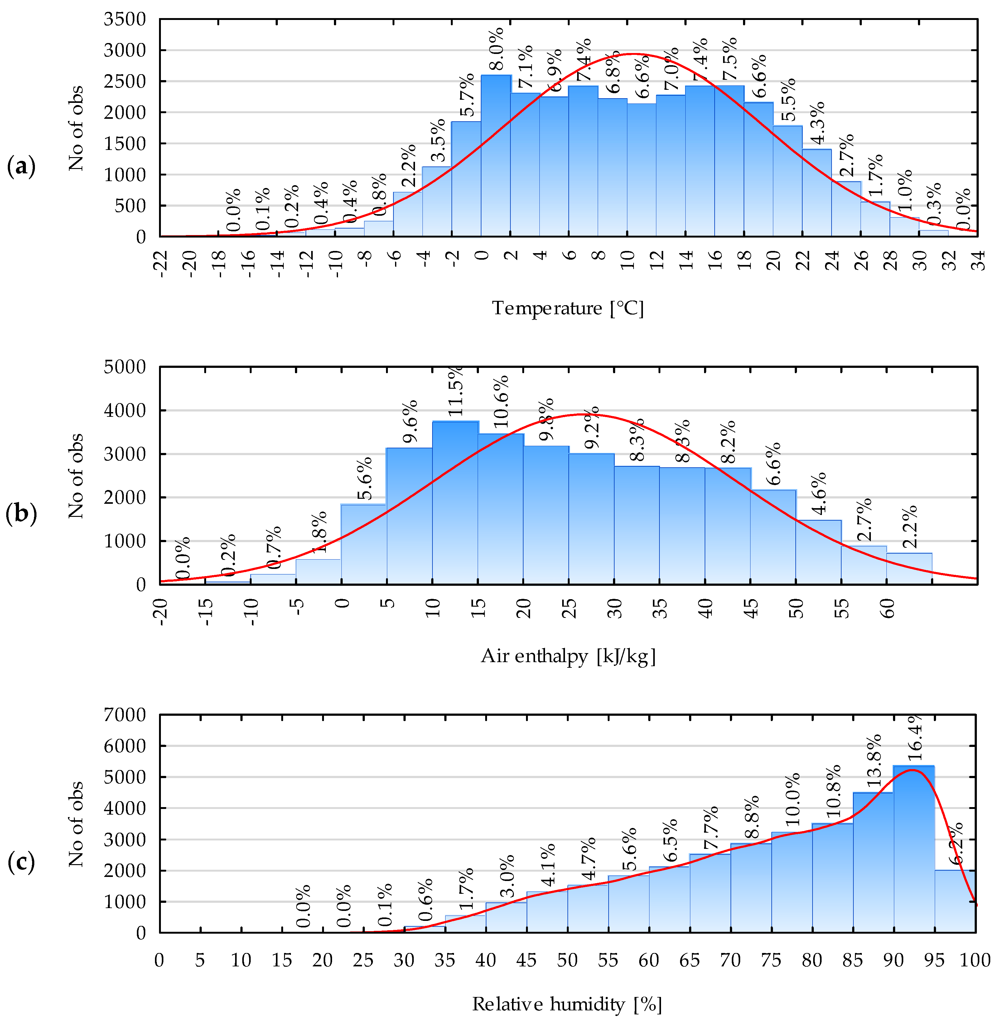
Outdoor air temperature significantly influences building heating demand. The most frequently observed temperature ranges are 0–2 °C (8.2%) and 14–18 °C (7.3% each). Figure 4 presents measurements from the entire monitoring period, not just the heating season. Lower frequencies are noted in the 2–14° C range (6.5–7.2%). Extreme temperatures below–14 °C occurred in less than 0.1% of the measurements.

The most frequently observed relative humidity range is 90–95%. Because relative humidity can be converted to absolute humidity only in relation to the corresponding air temperature, enthalpy—derived from temperature and humidity measurements—provides a more precise indication of thermal properties. While absolute humidity has minimal impact on enthalpy in winter due to low moisture content, in summer it becomes a critical factor because of the air’s higher moisture capacity. About 11% of the measured data fall within the 10–15 kJ/kg enthalpy range.

4.1.2. Solar Radiation

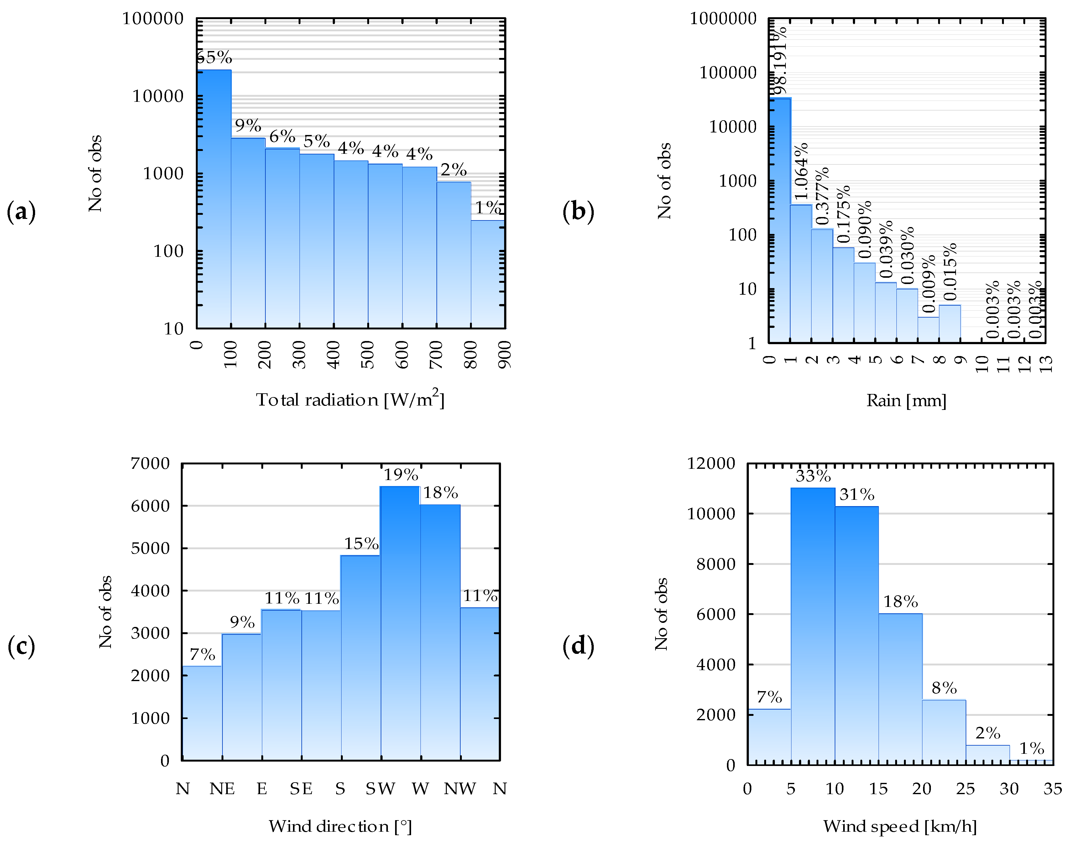
Total solar radiation, a critical factor for heat gains through glazing, is presented in 100 W/m² intervals (Figure 5a). Insolation in the 100–900 W/m² range decreases progressively. The 100–200 W/m² interval occurs 9% of the time, whereas higher intervals—such as 800–900 W/m²—represent only 1%. Nighttime radiation (0 W/m²) accounts for the largest share at 65%.

4.1.3. Rainfall

Rainfall (Figure 5b) is predominantly minimal, with 98.19% of the observations in the 0–1 mm range, encompassing both rainy and non-rainy periods. Heavier rainfall is rare, with amounts above 1 mm accounting for just over 1% of observations. This significantly affects air humidity and temperature.

4.1.4. Wind

At the studied location, winds predominantly originated from the W–SW (225–270°) and W–NW (270–315°) directions, accounting for 19% and 18% of the total measurement time, respectively. In contrast, the least frequent winds were from the N–NE (0–45°) and NE–E (45–90°) directions, occurring 7% and 9% of the time. The building’s exposure varies: it is sheltered by trees and neighboring buildings on the N–NE side, while on the S–SW side, it faces a narrow greenbelt and a city road.

Wind speeds were mainly low to moderate: the most common ranges were 5–10 km/h (33%, Beaufort scale 2, weak breeze) and 10–15 km/h (31%, Beaufort scale 3, gentle breeze). Air stillness or very low winds (0–5 km/h) were infrequent (7%), as were high speeds exceeding 25 km/h (3%).

Wind direction and strength are key determinants in forecasting thermal energy demand, particularly in Central Europe, where air masses from the east and northeast bring colder conditions, while those from the south and southwest result in warmer temperatures. General west-to-east circulation patterns dominate, but regional topography and land cover further influence wind flow and temperature distribution. Terrain roughness and obstacles like buildings or forests create localized variations, complicating predictions.

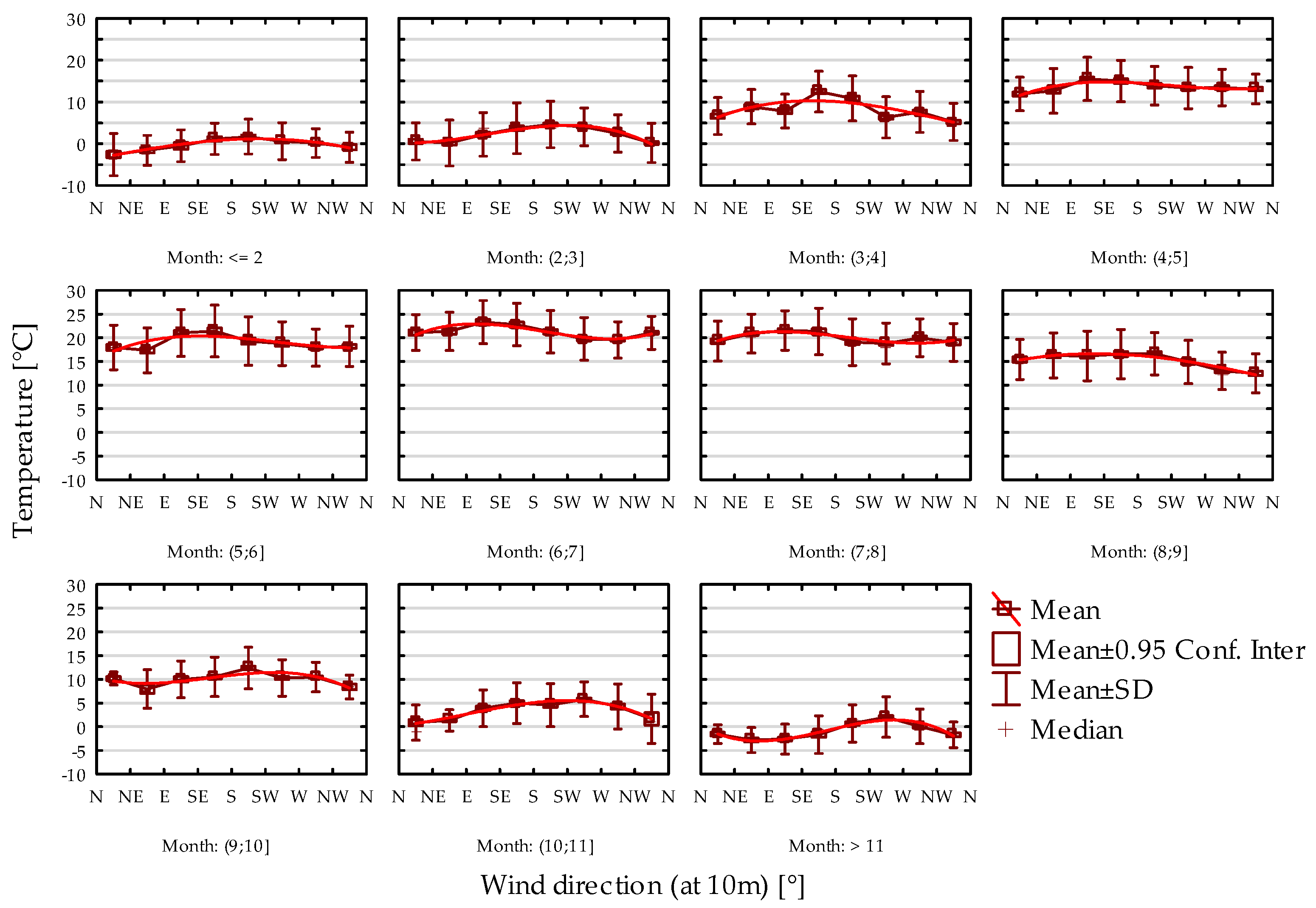
The graph in Figure 6 shows the dependence of mean outdoor temperature on wind direction by month for the location of the analyzed building. In the months November–March, noticeably lower average temperatures occurred for directions between NW and NE, while the warmest temperatures occurred for directions close to S-SW. However, this is not a clear phenomenon and is not similar for each location. The temperature fitting functions for wind directions by month, along with the statistics from the ANOVA test, are shown in

Table 1. Outdoor temperature fitting functions for wind directions by month and statistics according to the ANOVA test.

Month	Temperature t (°C)	Statistics
1, 2	t = −9.9172 + 3.3813·wd − 0.2128·wd2 − 0.0068·wd3	F(7;2968) = 36.486; p = 0.0000;
3	t = 3.5954 − 3.4682·wd + 1.0353·wd2 − 0.0748·wd3	F(7;5680) = 86.4379; p = 0.0000;
4	t = −5.9922 + 6.9825·wd − 0.8973·wd2 + 0.0301·wd3	F(7;2872) = 95.9659; p = 0.0000;
5	t = −1.5251 + 7.9374·wd − 1.2263·wd2 + 0.0583·wd3	F(7;2968) = 26.4546; p = 0.0000;
6	t = 4.3393 + 7.7112·wd − 1.1681·wd2 + 0.0533·wd3	F(7;2872) = 36.5684; p = 0.0000;
7	t = 4.9144 + 10.1994·wd − 1.8118·wd2 + 0.0963·wd3	F(7;2968) = 38.2703; p = 0.0000;
8	t = 7.062 + 7.9079·wd − 1.3798·wd2 + 0.0721·wd3	F(7;2968) = 23.4976; p = 0.0000;
9	t = 9.9154 + 3.1014·wd − 0.4083·wd2 + 0.0112·wd3	F(7;2872) = 45.6166; p = 0.0000;
10	t = 18.0339 − 6.1343·wd + 1.3155·wd2 − 0.082·wd3	F(7;2536) = 27.7323; p = 0.0000;
11	t = 0.4001 − 1.1533·wd + 0.6436·wd2 − 0.0535·wd3	F(7;2152) = 42.3006; p = 0.0000;
12	t = 15.801 − 12.0189·wd + 2.3888·wd2 − 0.139·wd3	F(7;2224) = 73.9223; p = 0.0000;

Note: w_d—wind direction.

. The p-value is less than the accepted significance level of 0.05, indicating that the differences in wind direction are statistically significant, and so have an impact on the temperature in each month.

4.2. Energy Characteristics of Building Depending on External Factors

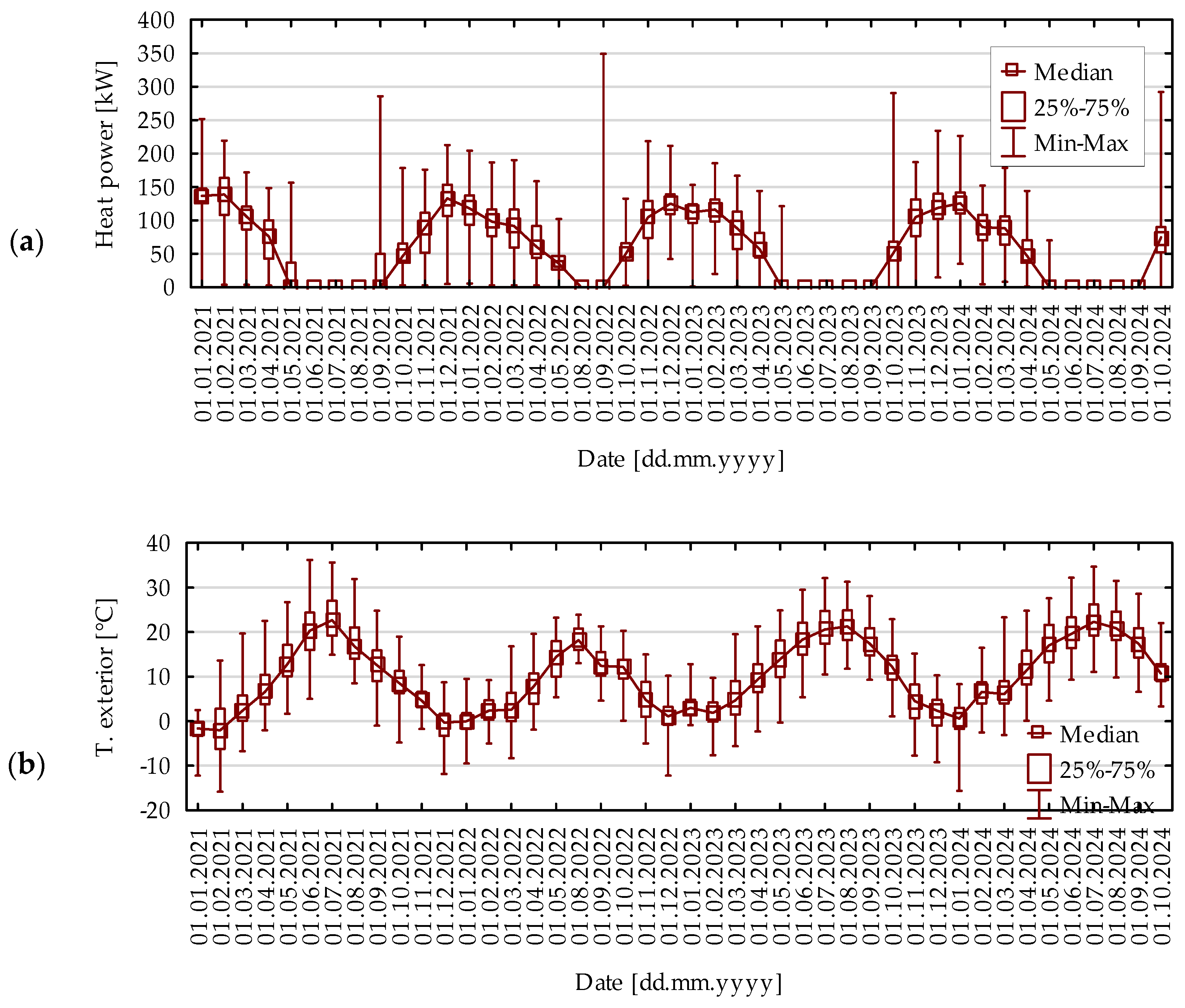
The analysis of energy consumption for heating the building reveals distinct patterns influenced by seasonal and operational factors. Figure 7 presents monthly energy consumption statistics, including median, interquartile range, and extremes. During summer (June–August), recorded energy consumption is zero, as the measurement system excludes energy supplied for domestic hot water.

4.2.1. Air Temperature and Enthalpy

In Poland, district heating typically commences when the average daily outdoor temperature remains below 12 °C for three consecutive days. The heating season usually starts in October, although in some cases, it may begin in late September. Similarly, the heating season ends in April or May when temperatures exceed 12 °C for three consecutive days. Decisions regarding heating schedules involve coordination between heating operators and building administrators, with flexibility to adapt to regional and climatic variations. Climate change has increasingly influenced the duration of heating seasons, necessitating adjustments to traditional schedules.

Energy demand is highest at the onset of the heating season, with instantaneous peaks reaching 300–350 kW, significantly exceeding the average demand of 92.75 kW by approximately 377%. This peak occurs during the start-up phase, when the heating medium temperature rises from room temperature (~20 °C) to the operational temperatures of 60–80 °C. December and January exhibit the highest average energy consumption, correlating with the coldest outdoor temperatures during these months. These observations underscore the critical relationship between outdoor temperature fluctuations, operational heating demands, and the need for dynamic energy management strategies.

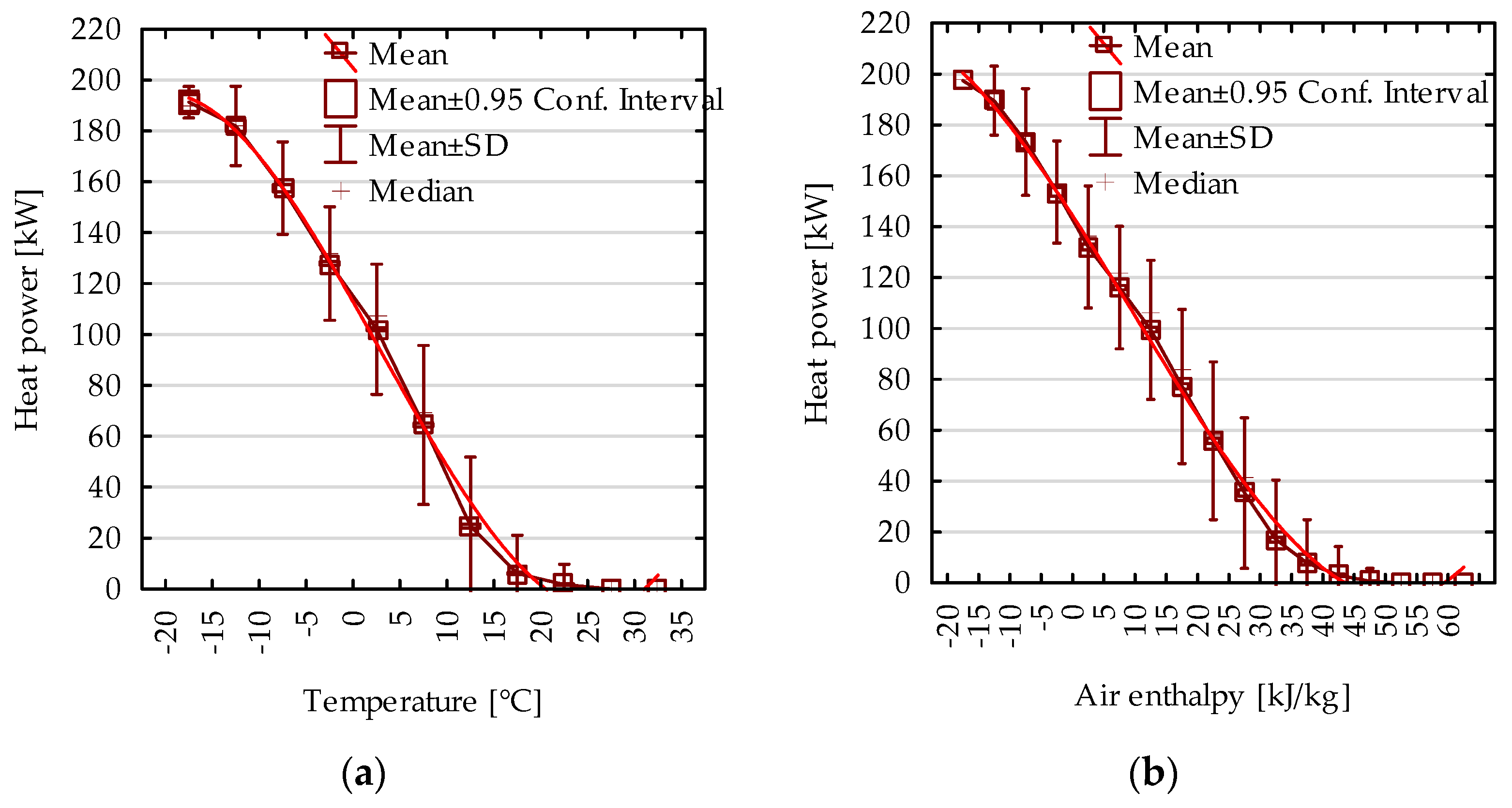
Figure 8 illustrates the relationship between energy consumption for heating and two key variables: outdoor temperature and enthalpy, encompassing the entire measurement period. As anticipated, a robust correlation exists between these parameters. Notably, within the temperature range of −10 °C to 10 °C, the relationship is approximately linear, indicating that as outdoor temperatures decrease, heating energy demand increases proportionally. However, when outdoor temperatures drop below −15 °C, this proportionality diminishes, suggesting that additional factors may influence energy consumption in more extreme cold conditions. Conversely, at temperatures exceeding 10 °C, there is a gradual decline in heating demand, reflecting reduced necessity for space heating.

The fitting functions of heat energy consumption on temperature and enthalpy are as follows:

$$\dot{\mathrm{Q}}=162.5626+34.5157·\mathrm{t}-10.2408·{\mathrm{t}}^2+0.5179·{\mathrm{t}}^3$$

$$\dot{\mathrm{Q}}=220.2905-3.3448·\mathrm{h}-2.1198·{\mathrm{h}}^2+0.0905·{\mathrm{h}}^3$$

The parameters of ANOVA test, respectively, F(10;29,147) = 12,627.2645, p = 0.0000 and F(16;29,185) = 7567.0628, p = 0.0000 indicate that the measurement results are statistically significant. The determination coefficient R² of the above relations equal 0.7443 and 0.6711, respectively.

This observed pattern aligns with established findings in building energy performance studies. For instance, research by Lee et al. [35] emphasizes the significance of determining accurate base temperatures for heating degree days to effectively estimate building heating energy consumption, underscoring the linear relationship between outdoor temperature and energy demand within specific temperature intervals. Furthermore, a study by Lin et al. [36] highlights that outdoor temperature accounts for a substantial portion of the variance in building energy consumption, reinforcing the critical role of ambient conditions in heating requirements.

The nonlinear function of heating energy demand described above offers advantages over traditional linear methods by providing a more accurate representation of energy consumption dynamics across a wide range of outdoor conditions. Understanding these dynamics is crucial for optimizing heating systems and enhancing energy efficiency. By incorporating higher-order functions (quadratic and cubic), the model captures the complex relationships between enthalpy and energy demand, including variations that linear methods fail to account for. This increased accuracy facilitates improved forecasting and optimization of energy systems, particularly under variable climatic conditions [37].

4.2.2. Wind and Solar Radiation

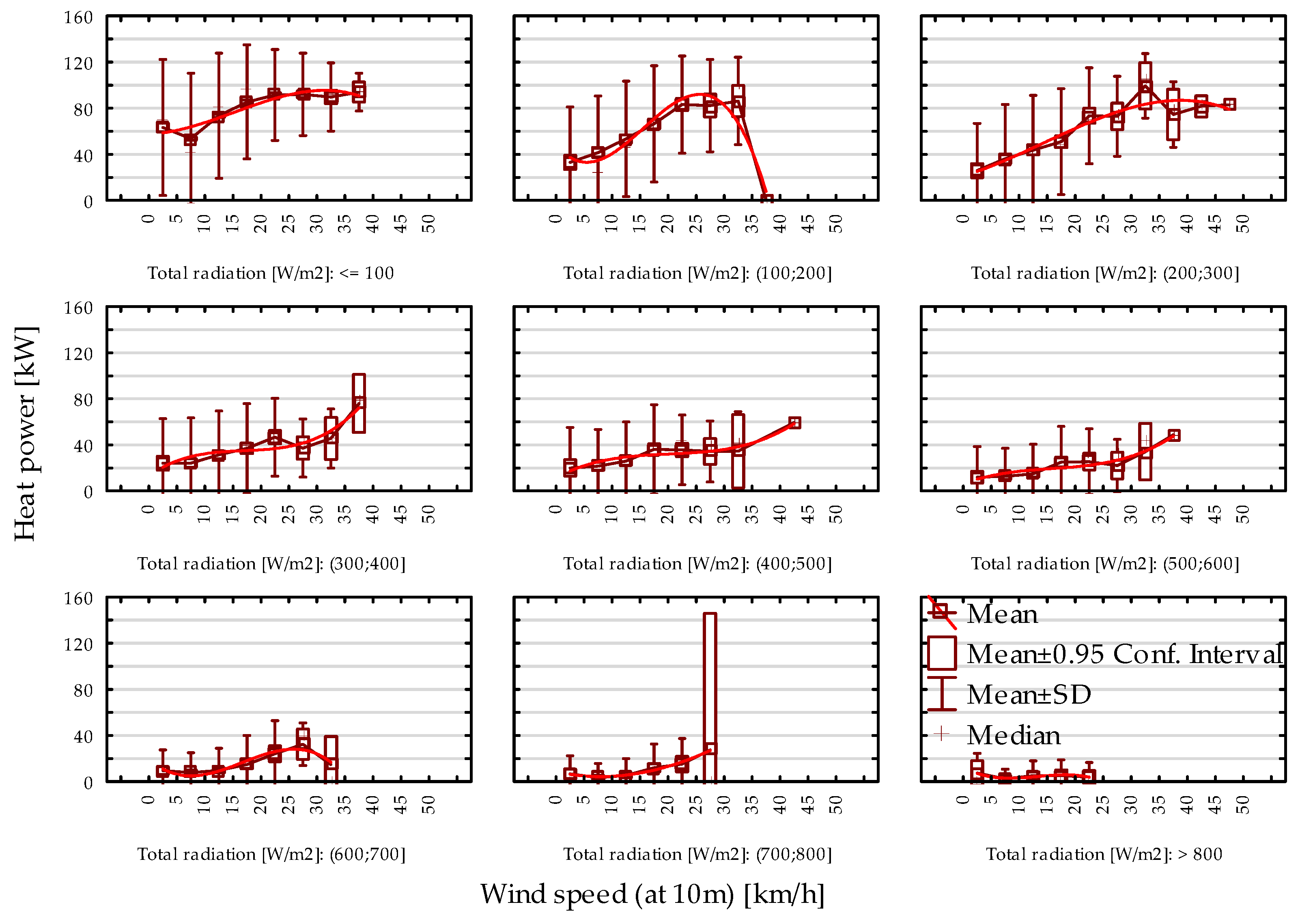
Wind significantly influences heating energy demand in the analyzed building by increasing heat loss through enhanced infiltration. To separate wind effects from solar radiation effects, the relationship between heating demand and wind speed was assessed across discrete solar radiation ranges (0–900 W/m², in 100 W/m² increments) (Figure 9). The ANOVA tests (

Table 2. Heat power demand fitting functions for wind speed on particular insolation category and statistics according to the ANOVA test.

Total Radiation (W/m2)	Heat Power Demand (kW)	Statistics
≤100	Q = 68.4317 − 12.8936·ws + 4.3066·ws2 − 0.2844·ws3	F(7;19,146) = 190.3894; p = 0.0000;
(100;200]	Q = 190.1537 − 118.5374·ws + 27.4408·ws2 − 1.7877·ws3	F(7;2548) = 35.6084; p = 0.0000;
(200;300]	Q = 13.1072 + 0.0362·ws + 2.3132·ws2 − 0.1581·ws3	F(9;1797) = 16.9779; p = 0.0000;
(300;400]	Q = −44.0105 + 41.8804·ws − 7.5847·ws2 + 0.4697·ws3	F(7;1509) = 8.0167; p = 0.00000;
(400;500]	Q = −28.0644 + 27.6231·ws − 4.3854·ws2 + 0.2417·ws3	F(7;1216) = 5.96; p = 0.00000;
(500;600]	Q = −23.8124 + 21.7412·ws − 3.8935·ws2 + 0.2523·ws3	F(7;1091) = 6.5308; p = 0.00000
(600;700]	Q = 108.0846 − 70.4099·ws + 14.9704·ws2 − 0.9354·ws3	F(6;1001) = 8.7824; p = 0.00000;
(700;800]	Q = 26.7597 − 12.9366·ws + 1.9848·ws2 − 0.0342·ws3	F(5;606) = 7.5585; p = 0.00000;
>800	Q = 69.8891 − 46.6696·ws + 10.5115·ws2 − 0.7535·ws3	F(4;176) = 0.5805; p = 0.6771;

Note: w_S—wind speed (km/h).

) revealed statistically significant relationships for insolation levels between 0 and 800 W/m², indicating that heat demand increases proportionally with wind speed under these conditions, as confirmed by regression analysis. However, for insolation levels above 800 W/m², no significant relationship was observed, as solar gains offset wind-induced heat losses. These findings emphasize wind’s role in building heat loss, particularly during periods of low solar radiation, consistent with prior research on wind-driven aeration effects [38].

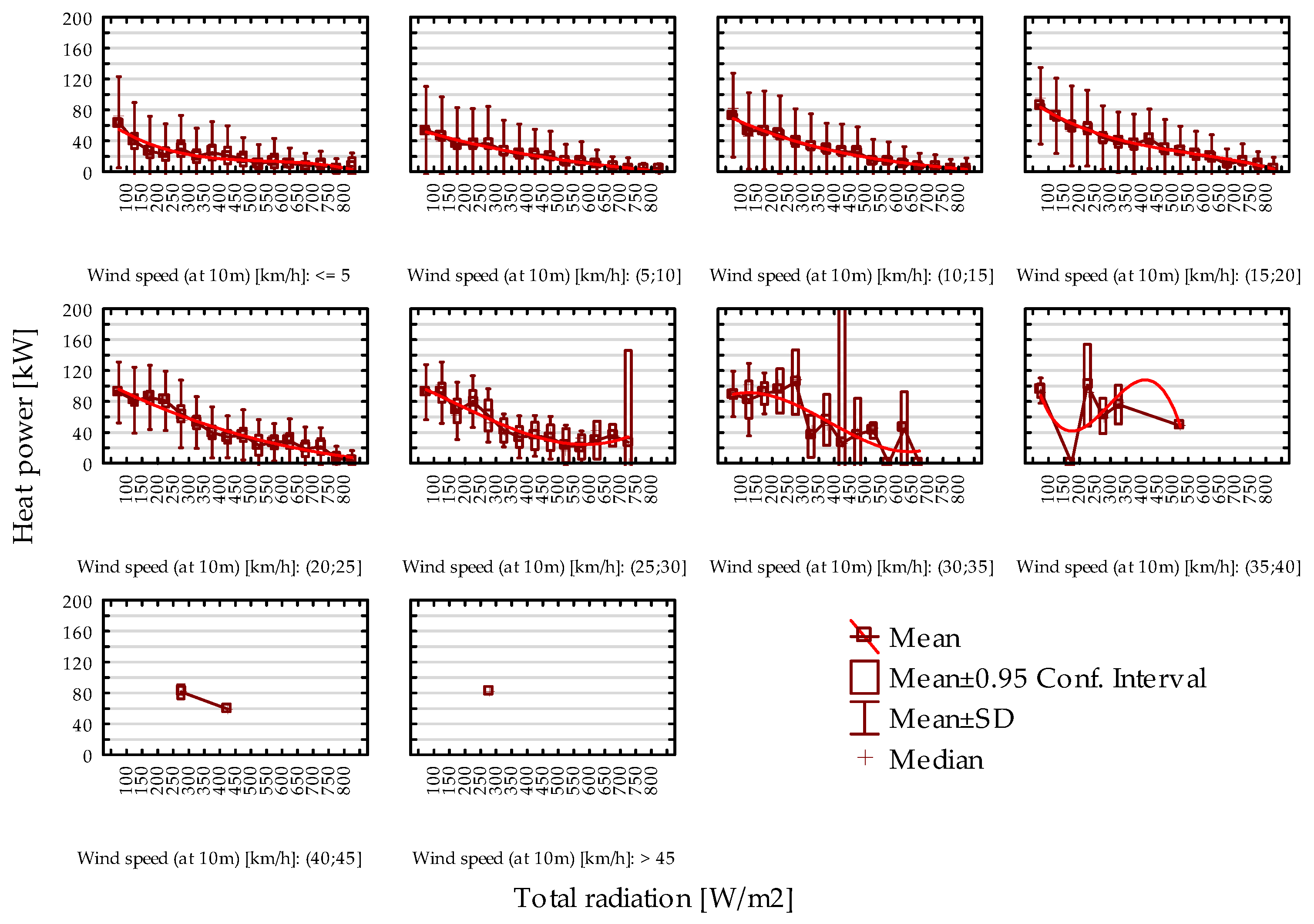
Figure 10 illustrates an inverse relationship between the total insolation and heating energy demand, analyzed across wind speed categories ranging from 0 to 50 km/h in 5 km/h intervals. The ANOVA test statistics (

Table 3. Temperature fitting functions for wind directions by month and statistics according to the ANOVA test.

Wind Speed Range (km/h)	Heat Power Demand Fitting Function	Statistics
(0;5]	Q = 73.2458 − 14.3344·it + 1.2206·it2 − 0.037·it3	F(15;1931) = 25.0244; p = 0.0000;
(5;10]	Q = 61.1676 − 6.5885·it + 0.2556·it2 − 0.0047·it3	F(15;9339) = 49.604; p = 0.0000;
(10;15]	Q = 83.1169 − 10.1643·it + 0.458·it2 − 0.0082·it3	F(15;9024) = 124.6993; p = 0.0000;
(15;20]	Q = 103.9029 − 15.1052·it + 1.0567·it2 − 0.0309·it3	F(15;5483) = 101.2037; p = 0.0000;
(20;25]	Q = 111.1267 − 10.6034·it + 0.3092·it2 − 0.0029·it3	F(15;2357) = 59.0748; p = 0.0000;
(25;30]	Q = 108.2153 − 7.9038·it − 0.4837·it2 + 0.0467·it3	F(13;717) = 17.1428; p = 0.0000;
(30;35]	Q = 76.0934 + 13.1959·it − 3.1656·it2 + 0.1376·it3	F(12;163) = 7.3227; p = 0.0000;
(35;40]	Q = 205.4494 − 108.7657·it + 22.0999·it2 − 1.2544·it3	F(5;25) = 8.7091; p = 0.00007;
(40;45]	Fit not drawn because of invalid range of values	-
(45;50]	Fit not drawn because of invalid range of values	-

Note: i_t—total insolation (W/m²).

) confirm the statistical significance of this relationship for wind speeds up to 35–40 km/h. Above 40 km/h, insufficient data precluded reliable analysis.

The observed inverse correlation aligns with the existing literature. Xie et al. [39] identified outdoor temperature, wind speed, and solar radiation as the key determinants of heating demand in district heating systems, noting that increased solar radiation reduces heating requirements. Similarly, a study by Song et al. [40] emphasized the impact of solar radiation and wind speed on building heating demand.

Wind speed’s influence on heating demand is multifactorial. Elevated wind speeds can enhance convective heat loss from building surfaces, increasing heating demand. However, high insolation can offset this effect by providing solar gains that reduce the need for additional heating. This relation was explored by Al-Homoud [38], who demonstrated that solar gains could compensate for heat losses due to wind-induced convection.

Our analysis indicates that at wind speeds above 35–40 km/h, the inverse relationship between insolation and heating demand diminishes. However, due to limited data at higher wind speeds, further research is necessary to substantiate this hypothesis.

Research underscores the complex interplay between wind speed and solar radiation in determining building heating demand. Understanding these dynamics is crucial for optimizing energy consumption and enhancing building energy efficiency.

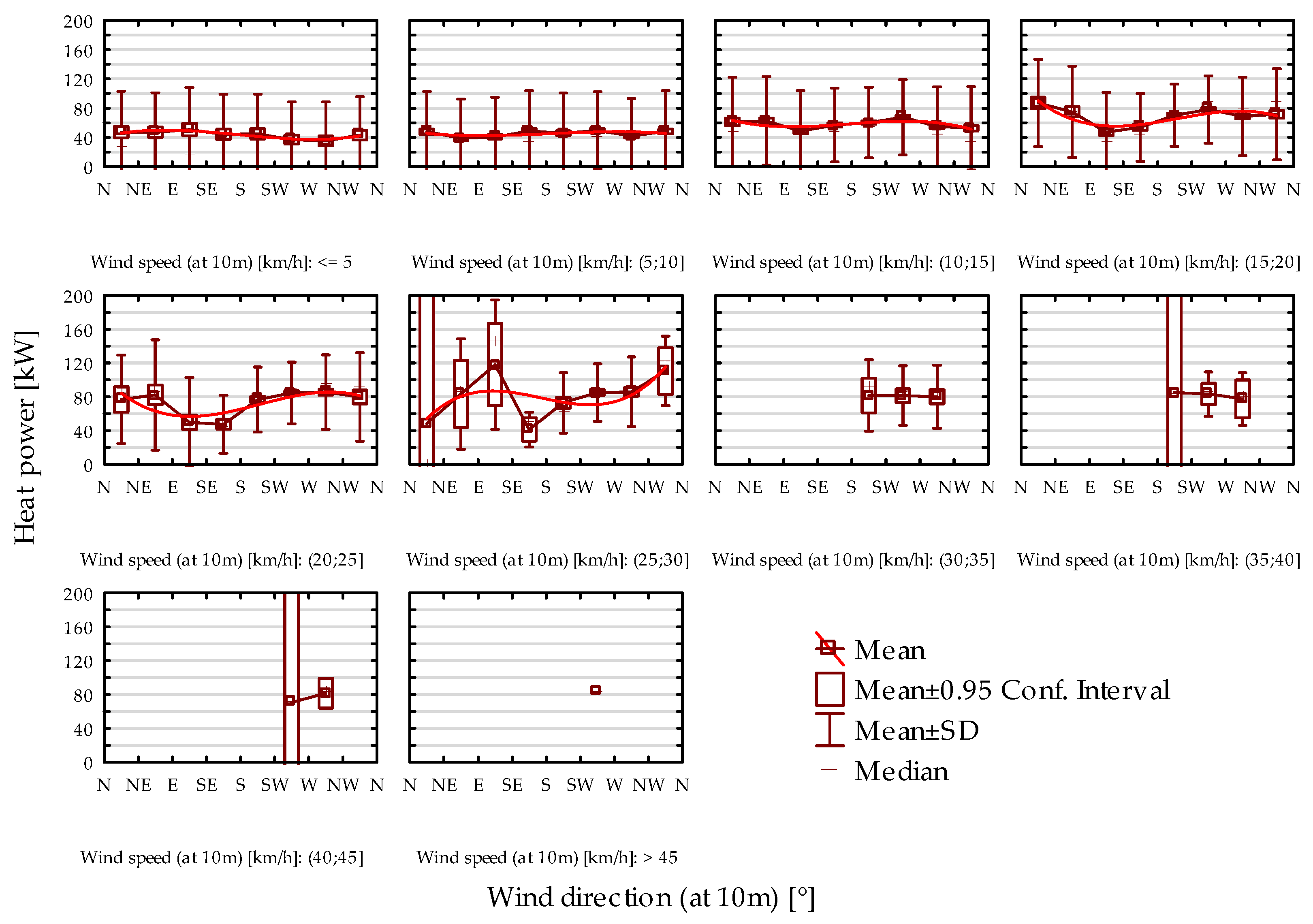
Figure 11 illustrates the relationship between heating energy consumption and wind direction across the determined wind speed categories.

Table 4. Heat power demand fitting functions for wind directions according to the determined wind speed category and statistics according to the ANOVA test.

Range	Fitting	Statistics
≤5	3.1295 + 29.3556·wd − 5.6688·wd2 + 0.317·wd3	F(7;1839) = 2.1315; p = 0.0376;
(5;10]	71.2418 − 16.8751·wd + 3.1059·wd2 − 0.1698·wd3	F(7;9447) = 7.018; p = 0.00000;
(10;15]	125.3444 − 40.83·wd + 7.4966·wd2 − 0.423·wd3	F(7;9032) = 16.0297; p = 0.0000;
(15;20]	257.4965 − 104.2522·wd + 17.1112·wd2 − 0.8653·wd3	F(7;5491) = 29.1478; p = 0.0000;
(20;25]	237.2269 − 96.6766·wd + 16.2979·wd2 − 0.8263·wd3	F(7;2365) = 23.6511; p = 0.0000;
(25;30]	−154.0297 + 136.3884·wd − 24.7527·wd2 + 1.4088·wd3	F(7;723) = 5.7929; p = 0.00000;
(30;35]	Fit not drawn because of invalid range of values	F(2;173) = 0.0332; p = 0.9673;
(35;40]	Fit not drawn because of invalid range of values	F(2;28) = 0.1572; p = 0.8552;
(40;45]	Fit not drawn because of invalid range of values	-
>45	Fit not drawn because of invalid range of values	-

Note: w_d—wind direction.

provides the corresponding heat power demand fitting functions and ANOVA test statistics. The analysis reveals that wind direction does not exhibit a significant impact on heating demand. However, at wind speeds exceeding 15 km/h, a slight reduction in heating demand is observed for south wind directions. The ANOVA test results include the F-statistic and p-values for each wind speed category. For instance, in the 15–20 km/h range, the F-statistic is 29.1478 with a p-value of 0.0000, indicating a statistically significant relationship between wind direction and heating demand. Conversely, for wind speeds above 30 km/h, the p-values exceed the typical significance threshold of 0.05, suggesting that any observed variations in heating demand across wind directions are not statistically significant in these higher wind speed categories.

These findings align with the existing literature on the impact of wind direction and speed on building heat energy consumption. Al-Homoud [38] emphasizes that wind can enhance convective heat loss from building surfaces, thereby increasing heating demand. However, the effect of wind direction is complex and influenced by building orientation and surrounding topography. Similarly, Xie et al. [39] identified wind speed as a significant factor affecting heating demand in district heating systems.

The observed reduction in heating demand for south winds at higher wind speeds may be attributed to the relatively warmer air masses from the south, which can mitigate heat loss. This phenomenon is supported by studies such as those by Taesler [41], who noted that wind direction should be included during building energy management, particularly in regions where southerly winds are warmer.

4.3. Prediction of Heat Demand Using ANN

Table 5. Summary of basic parameters of designated networks for prediction of thermal energy demand using standard meteorological parameters and additionally with weather forecasts.

ID	Net. Name	Training Accuracy (R2)	Testing Accuracy (R2)	Validation Accuracy (R2)	Training Algorithm	Error Function	Hidden Activation	Output Activation
Networks without temperature forecast
1	MLP 11-30-1	0.912142	0.900470	0.900538	BFGS 559	SOS	Logistic	Logistic
2	MLP 11-26-1	0.907722	0.897209	0.895392	BFGS 312	SOS	Tanh	Logistic
3	MLP 11-34-1	0.909786	0.896842	0.895216	BFGS 418	SOS	Logistic	Tanh
4	MLP 11-25-1	0.906600	0.895441	0.895890	BFGS 412	SOS	Logistic	Identity
5	MLP 11-35-1	0.910546	0.899098	0.896857	BFGS 339	SOS	Logistic	Logistic
Networks with temperature forecast
1	MLP 17-31-1	0.906588	0.895309	0.894706	BFGS 189	SOS	Logistic	Logistic
2	MLP 17-33-1	0.912256	0.898753	0.896136	BFGS 328	SOS	Logistic	Exponential
3	MLP 17-26-1	0.914544	0.898596	0.899251	BFGS 304	SOS	Tanh	Logistic
4	MLP 17-30-1	0.909190	0.897348	0.896592	BFGS 290	SOS	Logistic	Identity
5	MLP 17-33-1	0.910105	0.899107	0.897361	BFGS 267	SOS	Logistic	Tanh

specifies the architecture and learning details of each determined ANN. Performance is evaluated using training, test, and validation accuracy, where values closer to one indicate better predictive accuracy. For networks without temperature forecasts, the highest test accuracy (R² = 0.900470) is achieved by MLP 11-30-1, suggesting a well-generalized model. Among networks with temperature forecasts, MLP 17-33-1 exhibits a slightly lower test performance (R² = 0.899107), which is interesting given the inclusion of more predictive data.

The differences in performance between networks with and without temperature forecasts are subtle. The highest training performance among all the networks is observed in MLP 17-26-1 (R² = 0.914544). This suggests that while temperature forecasts improve training performance by potentially introducing additional predictive features, they do not necessarily translate to significantly better test or validation performance.

The determined ANN described in Table 5 differs in activation functions. For hidden layers, logistic and tanh functions are predominant, while output layers use logistic, tanh, identity, or exponential functions. These choices significantly influence the networks’ ability to model nonlinear relationships. Networks like MLP 11-35-1 (logistic-logistic) and MLP 17-33-1 (logistic-exponential) highlight the role of combining activation functions in enhancing performance.

The inclusion of temperature forecasts improves training performance, but the gains in test and validation accuracy are marginal. This is probably due to the correlation of some input variables to the forecasted temperatures. This redundancy highlights the need for the optimization of activation functions, training algorithms, and the application of advanced techniques, such as ensemble learning, to enhance model robustness and mitigate overfitting in networks with higher input dimensions [42].

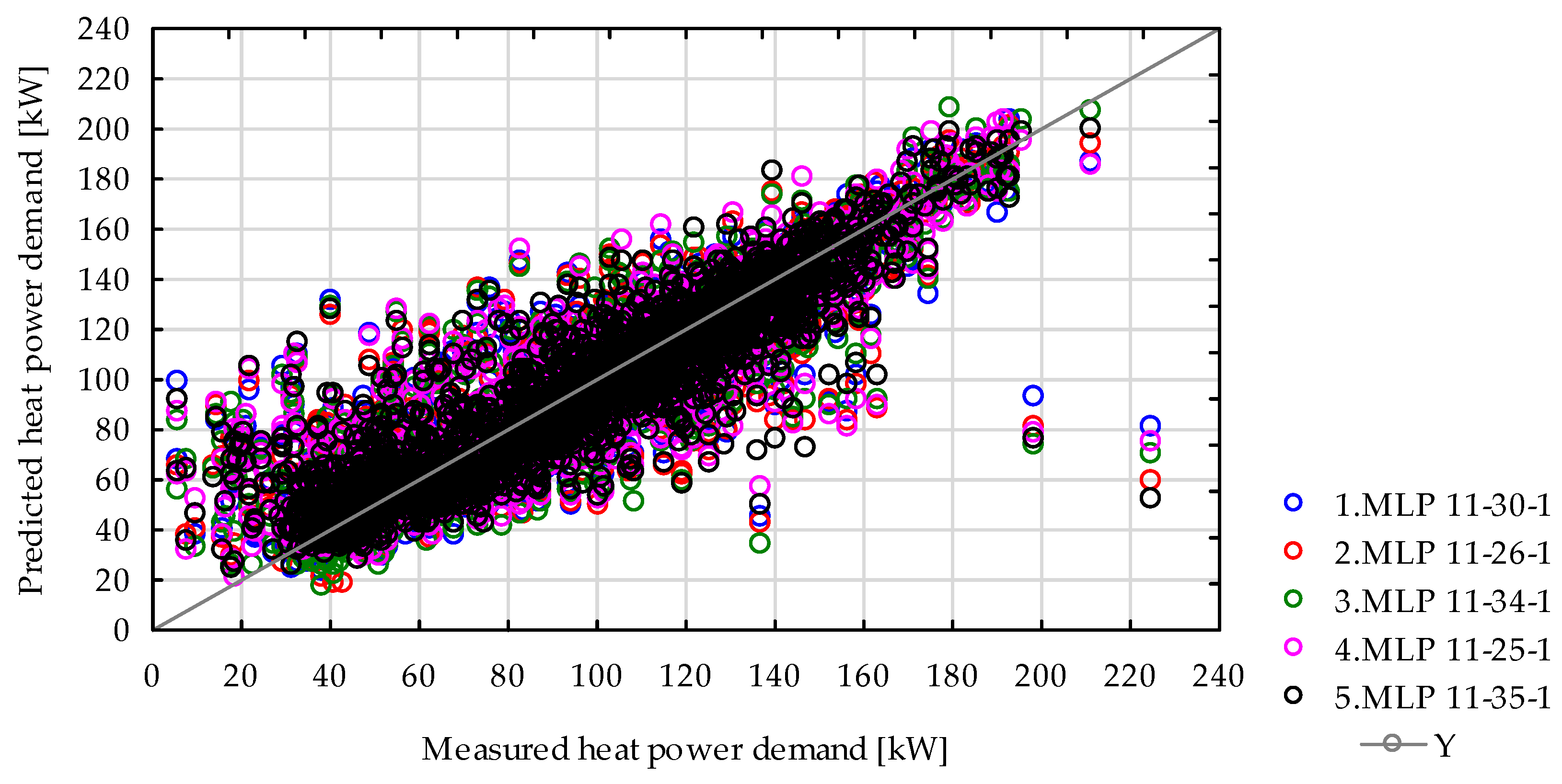
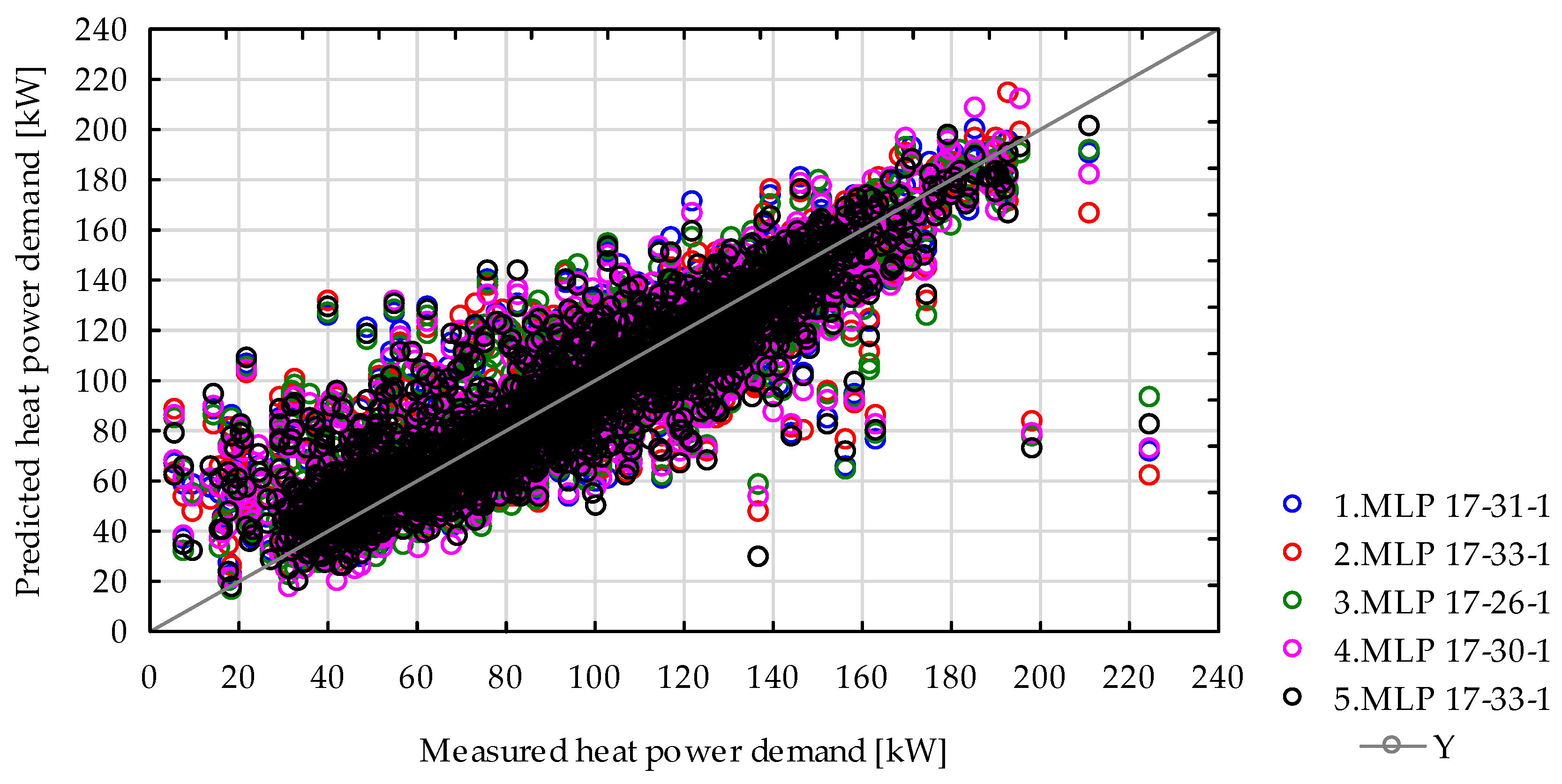
The diagrams in Figure 12 present the relationship between the thermal energy demand estimated by neural networks and the actual demand, offering a visual representation of the models’ performance. The upper graph illustrates the results from networks trained using standard meteorological parameters, while the lower graph presents the outcomes from networks that incorporated additional weather forecasts from 1 to 6 h ahead. Importantly, these graphs are based solely on validation data, ensuring an unbiased assessment of the networks’ predictive capabilities on data not involved in the training process.

The graphical analysis corroborates the performance coefficients outlined in the previous table. Specifically, the average validation determination coefficient (R²) for networks without temperature forecasts is 0.8967, while for networks utilizing forecast data, it marginally increases to 0.8968. This minor difference suggests that while adding the forecasted temperature data slightly improves model performance, the improvement is negligible.

The close fit observed in both graphs highlights the models’ ability to effectively capture the underlying patterns of thermal energy demand. The marginal advantage of including forecast data suggests that future work might focus on refining the integration of predictive variables, for example, by prioritizing forecasts with the highest impact on thermal demand dynamics. This refinement could help unlock the full potential of forecasted meteorological inputs in predictive modeling.

Table 6. Sensitivity analysis of particular inputs of neural networks.

Input Data	Temperature Forecast						Without Temperature Forecast
	1.MLP 17-31-1	2.MLP 17-33-1	3.MLP 17-26-1	4.MLP 17-30-1	5.MLP 17-33-1	Average	1.MLP 11-30-1	2.MLP 11-26-1	3.MLP 11-34-1	4.MLP 11-25-1	5.MLP 11-35-1	Average
Outdoor temperature text (°C)	2.276	2.412	2.344	2.505	2.213	2.350	3.614	3.803	3.391	2.916	3.584	3.462
Exterior air enthalpy hext (kJ/kg)	1.352	3.427	2.071	1.814	1.467	2.026	2.337	1.710	1.680	1.925	1.596	1.850
Total radiation (W/m2)	1.289	1.576	2.161	1.794	3.064	1.977	11.317	7.486	46.523	4.469	9.001	15.759
Direct radiation (W/m2)	1.036	1.536	1.909	1.807	3.303	1.918	9.600	6.541	58.298	2.701	8.906	17.209
Diffuse radiation (W/m2)	1.897	1.181	1.208	1.193	1.458	1.387	2.745	4.125	5.046	2.705	2.484	3.421
Wind speed ws (km/h)	1.060	1.098	1.152	1.088	1.063	1.092	1.189	1.196	1.274	1.179	1.184	1.204
Wind gust wg (km/h)	1.214	1.264	1.262	1.148	1.155	1.209	1.347	1.228	1.396	1.316	1.189	1.295
Wind direction wd (°)	1.026	1.010	1.043	1.038	1.022	1.028	1.067	1.029	1.037	1.019	1.063	1.043
Boundary layer height (m)	1.045	1.046	1.065	1.052	1.041	1.050	1.083	1.027	1.044	1.039	1.055	1.050
Month	2.734	5.033	1.422	3.794	8.856	4.368	1.552	1.912	2.851	1.538	4.601	2.491
Hour	1.452	1.296	1.283	1.407	1.444	1.376	1.398	1.288	1.518	1.209	1.446	1.372
Temp. forecast (°C): t+1h	1.650	2.186	2.439	2.679	2.492	2.289
Temp. forecast (°C): t+2h	2.033	2.159	1.435	1.526	1.421	1.715
Temp. forecast (°C): t+3h	1.600	2.681	1.912	3.111	1.364	2.133
Temp. forecast (°C): t+4h	1.679	1.893	1.587	2.347	3.546	2.210
Temp. forecast (°C): t+5h	1.248	1.793	1.531	1.498	1.098	1.434
Temp. forecast (°C): t+6h	1.762	1.384	1.209	2.232	1.585	1.634

presents a sensitivity analysis of the ANNs used for energy demand prediction, focusing on the importance of various meteorological inputs. The sensitivity values indicate each input’s influence on the network’s output, with higher values denoting greater impact. Sensitivity is determined by varying one input variable while keeping the others constant and observing changes in the output. The sensitivity unit does not match the units of the original variables because the software standardizes the variables during training. This ensures comparability across inputs with different scales or units.

For networks including temperature forecasts, the biggest impact appeared to be for the month code, namely 4.368. The outdoor temperature exhibits a moderate average sensitivity of 2.350, indicating its significant role in forecasting models. Exterior air enthalpy and total radiation follow, with the average sensitivities of 2.026 and 1.977, respectively. Among the forecasted temperatures, t_+1h has the highest sensitivity 2.289, with a gradual decline observed in longer-term forecasts, reaching 1.934 for t_+6h. This trend suggests that immediate temperature forecasts are more influential in predicting energy demand.

For networks excluding temperature forecasts, the outdoor temperature shows a higher average sensitivity of 3.462, underscoring its critical role when predictive data are absent. Total radiation exhibits a markedly high average sensitivity of 15.759, indicating a substantial reliance on this parameter. Direct radiation also shows significant sensitivity at 17.209, reflecting the network’s dependence on radiative inputs for accurate forecasting.

Incorporating meteorological inputs into ANN is crucial for accurately forecasting building energy demand. Recent studies emphasize the significance of variables such as outdoor temperature, enthalpy, and solar radiation. Lee et al. demonstrated that utilizing high-frequency temperature data enhances daily forecasting performance in neural networks [43]. Kumar and Elumalai identified air temperature and related parameters as dominant predictors in ANN models for temperature estimation [44]. Benavides Cesar et al. highlighted the importance of meteorological variables, including solar radiation, in improving ANN-based solar forecasting models [45].

5. Discussion

Meteorological parameters, including outdoor temperature, wind speed, solar radiation, and air enthalpy, have an important role in determining the thermal energy requirements of buildings. Among these, outdoor temperature is commonly acknowledged as the dominant factor influencing heating demand [35]. The data analyzed in this research corroborates this finding, showing a strong correlation between outdoor temperature fluctuations and heating energy consumption, especially within the range of −10 °C to 10 °C.

Wind speed and direction also significantly influence heat demand by affecting convective heat losses from building surfaces. The findings presented align with prior studies [38], which emphasize wind’s role in increasing energy loss, particularly under low-insolation conditions. Solar radiation, on the other hand, introduces a compensatory mechanism by providing passive heat gains that reduce the need for heating.

This finding is consistent with studies in urban contexts, such as Kittaka and Miyazaki, who reported that wind direction significantly influenced temperature distributions across different zones in Osaka [46]. Similarly, Lototzis et al. found a strong correlation between hourly wind directions and air temperature in Mediterranean climates, though their results suggest this relationship may diminish at broader time scales [47].

The impact of wind direction on temperature in this study further emphasizes the importance of understanding localized wind flow dynamics. Mizukoshi highlighted the role of advection in altering temperature distribution patterns in urban areas, which is also relevant to the regional conditions examined here [48]. The presence of obstacles such as buildings and forests, as noted in the study, can create localized variations in wind speed and direction, further modulating temperature. This is consistent with the findings by Hong-wei, who described complex interactions between wind direction and temperature over marine environments, suggesting that landforms and development may have an impact on meteorological parameters [49].

Furthermore, the study’s temperature fitting functions for each month provide valuable predictive insights, offering a means to model the effects of wind direction on temperature. These models can be utilized to optimize heating systems, allowing energy providers to respond dynamically to forecasted temperature variations. The application of artificial intelligence algorithms could enhance the accuracy of these predictions by identifying subtle, location-specific relationships that may not be plain.

ANNs have emerged as a powerful tool for predicting heat power demand due to their ability to model complex, nonlinear relationships inherent in meteorological and energy consumption data. In this study, multiple ANN architectures were tested, including configurations with and without predictive temperature data.

Despite the quite simple architecture of ANN, the accuracy is comparable to other research that utilizes a hybrid or ensemble analysis. Hybrid approaches presented by Dasi et al. show that integrated machine learning models with metaheuristic algorithms, such as the Satin Bowerbird Optimizer combined with extreme gradient boosting, have shown high coefficients of determination (0.938048) for heating load predictions, indicating superior performance with minimal error values [50].

A self-organizing map neural network was utilized by Dinmohammadi for feature dimensionality reduction, followed by an ensemble stacking classification model for energy consumption prediction. The stacking model achieved superior performance with an accuracy of 95.4% [51].

This study by Gong et al. employed a feedforward neural network (FFNN) optimized using a multi-tracker optimization algorithm (MTOA) to predict the annual thermal energy demand and weighted average discomfort degree hours in residential buildings. The proposed model achieved excellent accuracy, with a Pearson correlation coefficient exceeding 0.96, outperforming traditional methods and similar algorithms in both training and testing phases [52].

In research presented by Yamannage, a Neural Network Multi-Layer Perceptron (NN-MLP) achieved a high accuracy of 99.57% [53]. But, the target variable in this study, the heating load class, was not treated as a continuous variable like in our research, but was instead classified into three discrete categories: low, medium, and high. These findings underscore the effectiveness of machine learning algorithms, particularly ANNs, in accurately classifying heating load classes, contributing to improved energy efficiency in residential buildings.

The prediction of heat power demand using meteorological data and ANNs represents a significant advancement in energy forecasting. This research highlights the critical role of parameters such as temperature, wind speed, and solar radiation in determining thermal energy requirements, while also underscoring the potential of ANNs to model complex, nonlinear relationships. However, the findings also point to several areas where further refinement is needed, particularly in terms of feature selection, model regularization, and the integration of predictive data. By addressing these challenges, future studies can unlock the full potential of ANN-based forecasting systems, paving the way for more efficient and sustainable energy management practices.

ANN models are inherently specific to the datasets and conditions under which they are trained, limiting their applicability to the object or system of origin. Geographic and topographic variability introduces significant shifts in climatic conditions, such as temperature ranges, wind patterns, solar radiation intensity, and humidity levels, which influence energy dynamics. Furthermore, buildings exhibit unique thermal behaviors, governed by diverse heat loss/gain coefficients, material properties, insulation standards, and dynamic thermal response characteristics. These differences highlight the challenge of generalizing ANN models across varying contexts.

Future research should focus on identifying and standardizing critical climatic and building-specific factors that significantly influence thermal performance. By establishing universal indicators—such as normalized heat transfer coefficients or dimensionless performance metrics—it may be possible to develop generalized ANN frameworks. Such advancements could enable the cross-regional application of ANN models, improving scalability while maintaining predictive accuracy across diverse environmental and architectural frames.

Good results should also be obtained by taking into account internal factors that directly or indirectly affect the consumption of thermal energy, especially quantitative variables such as a representative internal temperature, or qualitative variables such as the characteristics of the residents (age and nature of the daily schedule).

6. Conclusions

The study analyzed four years of meteorological data to assess the impact of external factors on building thermal energy demand. Key variables included outdoor temperature, humidity, wind, and solar radiation.

The analysis of the relationships between energy consumption and energy demand for heating confirmed a strong influence of outdoor air temperature and enthalpy. These relationships are effectively described by third-degree polynomial functions, with determination coefficients (R²) of 0.7443 and 0.6711, respectively. Insolation in the range of 0–800 W/m², within specified wind speed ranges, was also found to have a significant impact. Furthermore, average wind speeds in the range of 0–40 km/h, within defined insolation ranges, were identified as influential. However, wind direction was determined to be statistically insignificant.

Neural networks are suitable for predicting the heat demand of retrofitted buildings. The average fit coefficient (R²) for networks without temperature forecasts is 0.8967, while for networks utilizing forecast data, it marginally increases to 0.8968. In thermally retrofitted buildings, the relationships between heat demand and individual meteorological factors are less distinct, with reduced wind impact due to improved building airtightness. Reduced solar radiation transmittance through windows decreases the risk of interior overheating in summer, lowering cooling demands, but on the other hand may also limit passive heat gains in winter, potentially increasing heating costs in some cases.

The sensitivity analysis highlights exterior temperature and solar radiation as critical inputs for ANNs in energy demand forecasting. For networks using temperature forecasts, the month index, current outdoor temperature, and 1–4 h forecasts are the most influential variables, with enthalpy also being significant. Direct and total radiation have slightly lower influences. For networks without forecasts, direct and total radiation dominate, followed by the current outdoor temperature and diffuse radiation, indicating varying input relevance based on forecast availability.

References

1. Chmielewski, J.M. Teoria Urbanistyki w Projektowaniu Miast i Osiedli; Wydawnictwo Politechniki Warszawskiej: Warszawa, Poland, 2001. (In Polish) [Google Scholar]
2. Bridgman, T.; Cummings, S.; Ballard, J. Who Built Maslow’s Pyramid? A History of the Creation of Management Studies’ Most Famous Symbol and Its Implications for Management Education. Acad. Manag. Learn. Educ. 2018, 18, 81–98. [Google Scholar] [CrossRef]
3. Zaniewska, H.; Kowalewski, A.T.; Thiel, M.; Barek, R. Zrównoważony Rozwój Osiedli i Zespołów Mieszkaniowych w Strukturze Miasta; Kryteria i Poziomy Odpowiedzialności; Instytut Rozwoju Miast: Kraków, Poland, 2008. (In Polish) [Google Scholar]
4. Erixno, O.; Abd Rahim, N.; Ramadhani, F.; Nor Adzmam, N. Energy management of renewable energy-based combined heat and power systems: A review. Sustain. Energy Technol. Assess. 2022, 51, 101944. [Google Scholar] [CrossRef]
5. Qayyum, F.; Jamil, H.; Ali, F. A Review of Smart Energy Management in Residential Buildings for Smart Cities. Energies 2024, 17, 83. [Google Scholar] [CrossRef]
6. Bansal, R.; Pandey, J. Load Forecasting Using Artificial Intelligence Techniques: A Literature Survey. Int. J. Comput. Appl. Technol. 2005, 22, 109–119. [Google Scholar] [CrossRef]
7. Ferdyn-Grygierek, J.; Sarna, I.; Grygierek, K. Effects of Climate Change on Thermal Comfort and Energy Demand in a Single-Family House in Poland. Buildings 2021, 11, 595. [Google Scholar] [CrossRef]
8. Zabrodin, A. The impact of temperature and relative humidity dependent thermal conductivity of insulation materials on heat transfer through the building envelope. J. Build. Eng. 2022, 46, 103700. [Google Scholar] [CrossRef]
9. Pakula, A. Zaangażowanie Odbiorców z Grup Gospodarstw Domowych w Zarzadzanie Popytem na Energię; Wydawnictwo Uniwersytetu Łódzkiego: Łódź, Poland, 2013; ISBN 978-83-7525-948-3. (In Polish). [Google Scholar] [CrossRef]
10. Filipini, M.; Zhang, L. Impacts of Heat Metering and Efficiency Retrofit Policy on Residential Energy Consumption in China. Environ. Econ. Policy Stud. 2019, 21, 203–216. [Google Scholar] [CrossRef]
11. Wang, Y.; Hivonen, J.; Qu, K.; Jakisolo, J.; Kosonen, R. The Impact of Energy Renovation on Continuously and Intermittently Heated Residential Buildings in Southern Europe. Buildings 2022, 12, 1316. [Google Scholar] [CrossRef]
12. Sadowska, B.; Piotrowska-Woroniak, J.; Woroniak, G.; Sarosiek, W. Energy and Economic Efficiency of the Thermomodernization of an Educational Building and Reduction of Pollutant Emissions—A Case Study. Energies 2022, 15, 2886. [Google Scholar] [CrossRef]
13. Gaweł, D. The technology that meets modern human needs—Criteria of assessment of smart home system. Teka Kom. Archit. Urban. Stud. Krajobraz. 2021, 17, 37–44. [Google Scholar] [CrossRef]
14. Felius, L.C.; Dessen, F.; Hrynyszyn, B.D. Retrofitting towards energy-efficient homes in European cold climates: A review. Energy Efficienc. 2022, 13, 101–125. [Google Scholar] [CrossRef]
15. Stokowiec, K.; Wcislik, S.; Kotrys–Dzialak, D. Innovative Modernization of Building Heating Systems: The Economy and Ecology of a Hybrid District-Heating Substation. Inventions 2023, 8, 43. [Google Scholar] [CrossRef]
16. Kumar, R.; Aggarwal, R.K.; Sharma, J.D. Energy analysis of a building using artificial neural networks: A review. Energy Build. 2013, 65, 352–358. [Google Scholar] [CrossRef]
17. Runge, J.; Zmeureanu, R. Forecasting energy use in buildings using artificial neural networks. Energies 2019, 12, 3254. [Google Scholar] [CrossRef]
18. Biswas, M.A.R.; Robinson, M.D.; Fumo, N. Prediction of residential building energy consumption: A neural network approach. Energy 2016, 117, 84–92. [Google Scholar] [CrossRef]
19. Karatasou, S.; Santamouris, M.; Geros, V. Modeling and predicting building’s energy use with artificial neural networks: Methods and results. Energy Build. 2006, 38, 949–958. [Google Scholar] [CrossRef]
20. Moayedi, H.; Mosavi, A. Double-target based neural networks in predicting energy consumption in residential buildings. Energies 2021, 14, 1331. [Google Scholar] [CrossRef]
21. Chen, S.; Ren, Y.; Friedrich, D.; Yu, Z.; Yu, J. Prediction of office building electricity demand using artificial neural network by splitting the time horizon for different occupancy rates. Energy AI 2021, 4, 100093. [Google Scholar] [CrossRef]
22. Amber, K.P.; Ahmad, R.; Aslam, M.W.; Kousar, A.; Usman, M. Intelligent techniques for forecasting electricity consumption of buildings. Energy 2018, 157, 886–893. [Google Scholar] [CrossRef]
23. Zhang, M.; Millar, M.A.; Chen, S.; Ren, Y.; Yu, J. Enhancing hourly heat demand prediction through artificial neural networks: A national-level case study. Energy AI 2024, 15, 100315. [Google Scholar] [CrossRef]
24. Ciulla, G.; D’Amico, A.; Brano, V.L.; Traverso, M. Application of optimized artificial intelligence algorithm to evaluate the heating energy demand of non-residential buildings at European level. Energy 2019, 176, 380–391. [Google Scholar] [CrossRef]
25. Jovanović, R.Ž.; Sretenović, A.A.; Živković, B.D. Ensemble of various neural networks for prediction of heating energy consumption. Energy Build. 2015, 94, 189–199. [Google Scholar] [CrossRef]
26. Simonovic, M.B.; Nikolic, V.; Petrovic, E.; Ciric, I. Heat load prediction of a small district heating system using artificial neural networks. Therm. Sci. 2016, 20, 1355–1365. [Google Scholar] [CrossRef]
27. Delgarm, N.; Sajadi, B.; Delgarm, S. Multi-objective optimization of building energy performance and indoor thermal comfort using artificial bee colony (ABC). Energy Build. 2016, 131, 42–53. [Google Scholar] [CrossRef]
28. Dahl, M.; Brun, A.; Andresen, G.B. Using ensemble weather predictions in district heating operation and load forecasting. Appl. Energy 2017, 193, 455–465. [Google Scholar] [CrossRef]
29. Protic, M.; Shamshirband, S.; Anisi, M.H.; Petkovic, D.; Mitic, D.; Raos, M.; Arif, M.; Alam, K.A. Appraisal of soft computing methods for short-term consumers’ heat load prediction in district heating systems. Energy 2015, 82, 697–704. [Google Scholar] [CrossRef]
30. Dey, M.; Gupta, M.; Turkey, M.; Dudley, S. Unsupervised learning techniques for HVAC terminal unit behavior analysis. In Proceedings of the 2017 IEEE SmartWorld, San Francisco, CA, USA, 4–8 August 2017; pp. 1–7. [Google Scholar] [CrossRef]
31. Gong, M.J.; Wang, J.; Bai, Y.; Li, B.; Zhang, L. Heat load prediction of residential buildings based on discrete wavelet transform and tree-based ensemble learning. J. Build. Eng. 2020, 32, 101455. [Google Scholar] [CrossRef]
32. Cholewa, T.; Siuta-Olcha, A.; Smolarz, A.; Muryjas, P.; Wolszczak, P.; Guz, Ł.; Bocian, M.; Balaras, C.A. An easy and widely applicable forecast control for heating systems in existing and new buildings: First field experiences. J. Clean. Prod. 2022, 352, 131605. [Google Scholar] [CrossRef]
33. Cholewa, T.; Siuta-Olcha, A.; Smolarz, A.; Muryjas, P.; Wolszczak, P.; Guz, Ł.; Bocian, M.; Sadowska, G.; Łokczewska, W.; Balaras, C.A. On the forecast control of heating systems as an easily applicable measure to increase energy efficiency in existing buildings: Long-term field evaluation. Energy Build. 2023, 292, 113174. [Google Scholar] [CrossRef]
34. National Geoportal. Available online: https://polska.geoportal2.pl (accessed on 1 December 2024).
35. Lee, K.; Baek, H.-J.; Cho, C. The Estimation of Base Temperature for Heating and Cooling Degree-Days for South Korea. J. Appl. Meteorol. Climatol. 2014, 53, 300–309. [Google Scholar] [CrossRef]
36. Lin, Y.; Huang, T.; Yang, W.; Hu, X.; Li, C. A Review on the Impact of Outdoor Environment on Indoor Thermal Environment. Buildings 2023, 13, 2600. [Google Scholar] [CrossRef]
37. Pergantis, E.N.; Al Theeb, N.; Dhillon, P.; Ore, J.P.; Ziviani, D.; Groll, E.A.; Kircher, K.J. Predictive heating controls: Field demonstrations in cold climates. Energy Efficienc. J. 2024, 360, 122820. [Google Scholar]
38. Al-Homoud, M.S. Performance characteristics and practical applications of common building thermal insulation materials. Build. Environ. 2005, 40, 353–366. [Google Scholar] [CrossRef]
39. Xie, J.; Ma, Z.; Guo, J. Impacts of Weather Conditions on District Heat System. arXiv 2018, arXiv:1808.00961. [Google Scholar]
40. Song, S.; Leng, H.; Xu, H.; Guo, R.; Zhao, Y. Impact of Urban Morphology and Climate on Heating Energy Consumption of Buildings in Severe Cold Regions. Int. J. Environ. Res. Public. Health 2020, 17, 8354. [Google Scholar] [CrossRef]
41. Taesler, R. Climate and Building Energy Management. Energy Build. 1991, 15–16, 599–608. [Google Scholar] [CrossRef]
42. Abdel-Aal, R.E. Hourly temperature forecasting using abductive networks. Eng. Appl. Artif. Intell. 2004, 17, 543–556. [Google Scholar] [CrossRef]
43. Lee, S.; Lee, Y.-S.; Son, Y. Forecasting Daily Temperatures with Different Time Interval Data Using Deep Neural Networks. Appl. Sci. 2020, 10, 1609. [Google Scholar] [CrossRef]
44. Kumar, A.; Elumalai, S.P. Application of artificial neural network to screen out the dominant meteorological parameters for prediction of air temperature. Earth Sci. Inform. 2023, 16, 3697–3716. [Google Scholar] [CrossRef]
45. Benavides Cesar, L.; Manso-Callejo, M.-Á.; Cira, C.-I. Three Novel Artificial Neural Network Architectures Based on Convolutional Neural Networks for the Spatio-Temporal Processing of Solar Forecasting Data. Appl. Sci. 2024, 14, 5955. [Google Scholar] [CrossRef]
46. Kittaka, K.; Miyazaki, H. Relationship between wind direction and air temperature in the Osaka center city determined using fixed point observation. Meteorol. Atmos. Phys. 2014, 9, 2. [Google Scholar]
47. Lototzis, M.; Papadopoulos, G.; Droulia, F.; Tseliou, A.; Tsiros, I.X. A note on the correlation between circular and linear variables with an application to wind direction and air temperature data in a Mediterranean climate. Meteorol. Atmos. Phys. 2018, 130, 259–264. [Google Scholar] [CrossRef]
48. Mizukoshi, M. A contribution to the relationships between the distribution of air temperature and the wind in an urban area. Geogr. Rev. Jpn. 1965, 38, 92. [Google Scholar] [CrossRef]
49. Lin, F.-J.; Wang, H.-G.; Leke, L.; Ni, H.-W. Influence of wind direction on characteristics of evaporation duct. J. Atmos. Oceanic Technol. 2007, 22, 410–413. [Google Scholar]
50. He, D.; Zhang, Y.; Bin, F.; Ashab, M. Proposing hybrid prediction approaches with the integration of machine learning models and metaheuristic algorithms to forecast the cooling and heating load of buildings. Energy 2024, 291, 130297. [Google Scholar] [CrossRef]
51. Dinmohammadi, F.; Han, Y.; Shafiee, M. Predicting Energy Consumption in Residential Buildings Using Advanced Machine Learning Algorithms. Energies 2023, 16, 3748. [Google Scholar] [CrossRef]
52. Gong, Y.; Zoltán, E.S.; Gyergyák, J. A Neural Network Trained by Multi-Tracker Optimization Algorithm Applied to Energy Performance Estimation of Residential Buildings. Buildings 2023, 13, 1167. [Google Scholar] [CrossRef]
53. Yamannage, S.N. Heating Load Class Prediction in Residential Buildings: A Machine Learning Approach for Enhanced Energy Efficiency. TechRxiv 2024. [Google Scholar] [CrossRef]
Figure 1. Diagram of the conducted analysis presented in this article.
Energies 18 00679 g001
Figure 2. Forecasting controller: (a) schema of connection forecasting controller installed on existing heat exchanger room; (b) view of forecast controller mounted on tested installation.
Energies 18 00679 g002
Figure 3. The location of the analyzed multi-family residential building in relation to its surroundings (on the basis of polska.geoportal2.pl (accessed on 10 December 2024) [34]).
Energies 18 00679 g003
Figure 4. Histogram illustrating the frequency of measured parameters within specified ranges: (a) temperature, (b) air enthalpy, and (c) relative humidity.
Energies 18 00679 g004
Figure 5. Summary of meteorological data during measurement periods: (a) total radiation, (b) rainfall, (c) wind direction, and (d) wind speed.
Energies 18 00679 g005
Figure 6. Dependence of the mean outdoor temperature on wind direction by month for the given location.
Energies 18 00679 g006
Figure 7. Results of measurements: (a) heat energy demand; (b) outdoor temperature.
Energies 18 00679 g007
Figure 8. Dependence of energy consumption for heating on (a) outdoor air temperature and (b) enthalpy of outdoor air.
Energies 18 00679 g008
Figure 9. Dependence of heating energy consumption on wind speed determined for each total insolation category.
Energies 18 00679 g009
Figure 10. Dependence of heating energy consumption on total insolation determined for each wind speed category.
Energies 18 00679 g010
Figure 11. Dependence of heating energy demand on wind directions according to speed category.
Energies 18 00679 g011
Figure 12. Comparison of estimated vs. actual demand: top graph uses typical meteorological parameters, and bottom graph includes 1–6 h weather forecasts.
Energies 18 00679 g012aEnergies 18 00679 g012b