Electricity Price Volatility and the Performance of Machine Learning Forecasting Models in European Energy Markets

Abstract

Electricity is fundamental to the functioning of modern economies, yet its price volatility presents significant challenges for both long-term investment planning and short-term operational decision-making. In this study we examine electricity price dynamics across seven diverse European bidding zones, selected through principal component analysis to reflect a broad spectrum of energy mix characteristics. The analysis explores the relationship between the structure of national energy mixes—classified according to the controllability of generation sources—and the volatility and predictability of electricity prices during 2023–2024. Using ENTSO-E data, adaptive machine learning models were developed to forecast day-ahead electricity prices, with the Random Forest algorithm consistently achieving the highest predictive accuracy. The results indicate that bidding zones dominated by low-controllability renewable generation exhibit greater price volatility and reduced forecast accuracy, whereas zones with a higher share of controllable sources, such as natural gas, demonstrate more stable prices and improved model performance. These findings underscore the crucial role of the energy mix composition in shaping market dynamics and highlight the necessity of adopting adaptive, mix-sensitive forecasting methodologies in increasingly diversified electricity systems.

1. Introduction

Our civilization is fundamentally dependent on a stable and reliable supply of electricity. Even short-term interruptions in electricity availability can cause severe disruptions to both economic activity and social life. Electricity, however, is a commodity that is difficult to store in large volumes. Its generation must continuously match demand, while its production and distribution rely on complex systems that are inherently vulnerable to a variety of risks [1]. These characteristics make electricity markets highly sensitive to disturbances, with prices often displaying substantial variability and volatility [2,3]. To mitigate such risks, policymakers and operators introduce stabilizing mechanisms, such as cross-border electricity transmission and market integration. Nevertheless, sudden supply–demand imbalances frequently result in sharp price spikes or drops, threatening the stability of the energy system and occasionally leading to forced outages (blackouts).

On the other side, accurate forecasting of electricity demand and prices—both in the short and long term—is therefore essential for energy producers, market operators, policymakers, and consumers. Price surpluses can result in steep declines in market value, whereas shortages can drive significant increases; both extremes undermine system stability and market confidence [4]. Reliable forecasts can help stakeholders optimize production planning, balance supply and demand, mitigate risk exposure, and inform regulatory decision-making.

Despite the importance of accurate forecasting, electricity prices remain difficult to predict due to their volatility, nonlinear dynamics, and the influence of multiple exogenous factors such as weather, policy changes, and geopolitical events [1,5]. Volatility and sensitivity to political, economic, and social conditions are permanent features of fuel and energy markets. Prices change over longer periods of time and experience large, albeit short-lived, fluctuations [6]. In recent years, machine learning (ML) methods have attracted growing attention in the literature as promising tools for capturing such complexity.

Although the literature provides a wealth of models for both volatility analysis and price forecasting, few studies explicitly investigate how market volatility influences the accuracy of ML-based forecasting approaches. This gap motivates our study, which aims to analyze electricity price volatility across selected European markets and assess its impact on the predictive performance of ML algorithms and evaluate how volatility itself impacts the predictive performance of these models in real-world energy markets.

In view of these challenges, this article investigates the phenomenon of electricity price volatility within selected market zones of the European energy system. The selection of the European market for this study was motivated by several key factors related to its complexity, integration, and inherent challenges. As the largest interconnected electricity network in the world, it exhibits substantial diversity in climate, weather patterns, price characteristics, and energy mix structures across its regions, while also being influenced by geopolitical and social factors. These features make the European market an ideal setting for assessing the impact of price volatility on the performance of adaptive machine learning models.

The article further examines the relationship between volatility and the predictive accuracy of forecasting models based on machine learning algorithms, thereby contributing to the growing body of research on data-driven energy market forecasting. The main contribution of this article is to demonstrate, with statistical justification, the relationship between market volatility—measured as electricity price fluctuations—and the accuracy of forecasts delivered by ML models. This study also statistically substantiates the links between the energy mix, volatility indicators, and the performance of predictive models.

The present study is the next stage of the team’s research [7], extending previous work on machine learning forecasting from the Polish market to multiple European markets, with different objectives and datasets.

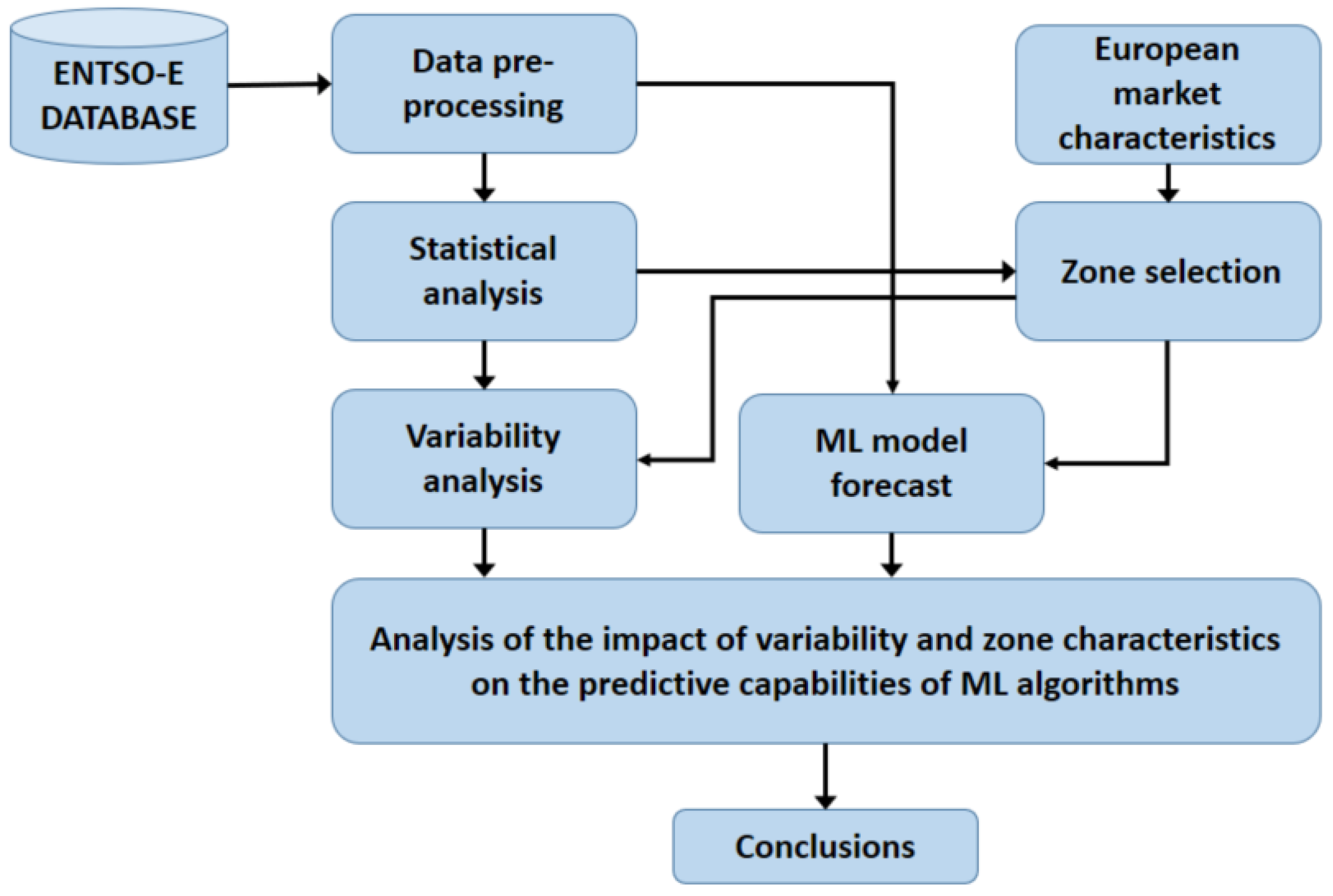
The outline of the study is as follows (see also Figure 1): the next section presents the background of the study and related works, while the third section presents the characteristics of selected zones of the European energy market and a detailed statistical analysis of price volatility in these zones. Section 4 presents the assumptions and methodology for developing four predictive models using ML algorithms for selected zones, and shows and compares their performance results. In Section 5 we analyze and discuss the interdependence between price volatility, forecast quality, and energy mix. The final Section 6 contains conclusions, limitations and indications for further work.

2. Research Background and Related Works

Electricity price forecasting is a critical component of energy market operations, enabling stakeholders such as utilities, traders, and regulators to make informed decisions regarding production, consumption, and risk management. Due to the non-storable nature of electricity and the influence of numerous dynamic factors, such as weather, demand fluctuations stemming from social phenomena, fuel prices, and grid technical constraints, forecasting of electricity prices is inherently complex. Accurate predictions are essential for optimizing bidding strategies, ensuring grid stability, and minimizing financial exposure in both day-ahead and intraday markets.

2.1. Volatility

Variability (volatility, dispersion) measures in statistics (from a static point of view) describe the volatility of analyzed empirical distributions. The most popular measures are range (R), interquantile range (IQR), standard deviation (sd) and the coefficient of variation (V). The formulas for the measures used in the text are presented in the Appendix A. These metrics (in static interpretation) were applied to describe variability of prices in [8,9].

In variability analyses on financial and commodity markets, variables related to time-variability are used. These include variables describing the daily scope of variability during the day (intraday volatility), indexed by hour index h ranging from 0 to 23 [10,11].

$$I{R}_D=\underset{h}{max}{P}_D-\underset{h}{min}{P}_D,$$

(1)

In most works related to price forecasting and risk analysis, measures of volatility are calculated on the basis of relative changes, most often daily linear or logarithmic rates of return [12,13,14].

In the case when prices are negative or equal to zero, absolute differences are considered [15,16].

$$A{I}_{D,h}=P_{D,h}-P_{D-1,h},$$

(2)

where $P_{D,h}$—price in the h-th hour of the day D, $P_{D-1,h}$—price in the h-th hour of the day $D-1$, for $h=0,\dots ,23$.

In the analysis of relative price changes, apart from logarithmic rates of change, linear relative differences are also used. They may be applied to negative prices, accounting for the sign of change. Moving averages are often used in that role [15]. Due to the presence of zero-valued prices, the weekly average price calculated the day before (that is for $D-1$) was used for normalization.

$$R{I}_{D,h}={\displaystyle \frac{P_{D,h}-P_{D-1,h}}{|mw{P}_{D-1}|}},$$

(3)

where $mw{P}_{D-1}$ denotes mean weekly price one day ago.

The increase in electricity prices and their growing volatility have been observed worldwide in recent years [17]. However, the scale of the price surge and the extent of volatility in the European market, particularly in the years 2022–2024, have reached alarming levels which, according to economists, are already exerting a clear and adverse impact on the economies of European countries [18]. Hence, price volatility in the electricity market is the subject of numerous studies [9,16,19,20]. The analysis of price volatility is now increasingly linked to the share of individual sources in the total production. Maciejowska [8] used quantile regression to analyze the impact of renewable energy sources (RESs) on price distributions for the German market. The authors of [9] show that the growing integration of RESs in Germany, France, Slovakia, the Czech Republic, Poland and Estonia—especially wind and solar energy—has a significant impact on the dynamics of electricity price changes. The authors of [21] demonstrate that for selected US states, the volatility of electricity prices is negatively correlated to increases in the amount of gas produced. Based on research on the German electricity market in 2015–2023 [22], two main trends in future price changes were identified. It was noted that the development of renewable energy contributes to lower electricity prices. The phase-out of nuclear energy, the rising price of CO₂ emission allowances and the higher price of gas contribute to price increases. Furthermore, higher price volatility reduces the quality of forecasts regardless of the methods used for all analyzed markets [23,24].

2.2. Energy Price Forecasting

A myriad of works address the topic of energy price forecasting (EPF), and there are many approaches to EPF. They can be classified as econometric, machine learning, or hybrid models. The most popular approaches within the first class are linear ARIMA models [25] and nonlinear GARCH models [12,26]. Hybrid methods, combining ARIMA with GARCH, have also been employed to jointly capture temporal dependencies and volatility effects [26,27]. However, despite their interpretability and solid statistical foundation, these methods often struggle with the nonlinear and high-dimensional structure of electricity markets. The main difficulty in using these models is also the need to use many parameters and strong assumptions about the distribution of variable values.

An alternative to econometric approaches are methods based on ML algorithms. Their main advantage is the ability to include nonlinear relationships between variables in the predictive model and, in the case of some methods, to simultaneously use numerical and categorical variables. While ML methods offer higher flexibility and accuracy, they have their own limitations. Their performance often strongly depends on hyperparameter tuning, computational resources, and the availability of large datasets. Despite this, in most comparative studies, these models showed better results than econometric models [28,29]. An important advantage of ML methods over parametric models such as ARIMA is also that parametric models impose conditions on the distributions of variable values. ML algorithms do not require either a specific distribution or linearity. Due to their speed, they can be quickly and easily recalibrated when new variables appear or when variables begin to take on different values than earlier. All these features make them very popular tools of classification and prediction. For instance, due to its advantages, Random Forest (RF) has been used in many studies also related to predictions in the energy market, e.g., [30,31,32,33]. In work on the possibilities of using ML methods in EPF, Support Vector Regression (SVR) and k-Nearest Neighbor (kNN) Regressor algorithms were also examined [34,35,36,37,38,39]. The kNN method, on the other hand, was presented in [40,41]. In addition to classic machine learning algorithms, research is being conducted on the use of various types of neural networks in EPF. They allow for the inclusion of complex relationships between variables, do not require any assumptions about the distribution of variables, and provide results that are comparable or slightly better than classic ML models (see, e.g., [42,43,44]). Their disadvantages include high requirements for the amount of training data, the need to select the right architecture and learning parameters, and difficulties in explaining the results obtained. A new trend is the use of generative artificial intelligence and LLMs (Large Language Models) to implement or support EPF [45,46,47].

The basic principle behind forecasting models is the assumption that the future will be similar to the past. As this assumption is valid only when the system is stable, in situations where anomalies occur, the quality of the forecast deteriorates rapidly [48]. To improve the predictive performance of ML models when the market is highly volatile, researchers’ efforts focus on model modifications or appropriate preparation of input data [49]. A widely used technique in EPF is combining different predictive models (both statistical and machine learning) to leverage the best features of each and improve forecast quality. This approach can work better, especially for complex systems. In general, an ensemble learning model will perform better than any single learning model if the proper ensemble strategy is applied. Examples and an overview of approaches for constructing hybrid EPF models can be found, among others, in [50,51,52,53,54].

Another approach involves enriching the input dataset and including additional variables whose presence improves the forecast. For instance, study [48] analyzed three European markets—France, Germany, and Belgium—in the period 2011–2016 for day-ahead market prices, using RF and Decision Tree (DT) machine learning methods. The results showed that taking into account data from neighboring markets significantly improves the quality of forecasts. The impact of market conditions on the quality of EPF is also shown in [55], where, based on data from the day-ahead market in Germany and Finland, the variation in forecast quality depending on the price category (normal, high, and negative) is demonstrated. The usefulness of ML in short-term hourly price forecasting, based on meteorological data, is demonstrated in [56]. In [31], it was experimentally proven that in time-series prediction tasks, using a small number of recently observed input variable values in the ML algorithm leads to improved algorithm accuracy. Therefore, one of the key steps of the entire procedure is determining the length of the time window that the algorithm will cover. Analogous conclusions were presented in [57], where prices on the day-ahead market in three countries—Greece, Belgium and Ireland—were examined using four ML algorithms. Among the various insights obtained, it was shown that forecasts derived from a relatively short historical window (45–60 days) can be effective, and that it is also possible to construct models capable of capturing sudden price movements. All of the above findings suggest that short-window training approaches can effectively improve forecasting models in volatile market terms. Similar results were shown in [7], where the best results in EPF were achieved by an RF model covering only the previous 8 days.

2.3. European Market Characteristics

The European electricity market has been undergoing institutional and technical integration for several decades. The integrated European energy market currently consists of 40 Transmission System Operators (TSOs), representing 36 countries, making it the largest interconnected electrical grid in the world. All TSOs are associated within ENTSO-E (the European Network of Transmission System Operators for Electricity), to provide secure and coordinated operation of Europe’s electricity system. As a result, it creates a system which, on the one hand, provides mutual support for market participants and improves network stability, but on the other hand increases its complexity [58,59].

From a technical perspective, the European electricity market is divided into so-called bidding zones (BZs). In line with [60], BZs must be delineated to support effective congestion management and promote overall market efficiency. Furthermore, ref. [61] states that BZ borders should reflect long-term, structural congestion within the transmission network. Structural congestion should not exist within a bidding zone unless either it has no impact on adjacent zones or, as a temporary exception, its effects are mitigated through remedial actions. European BZs use a uniform pricing mechanism in their day-ahead electricity markets, meaning all participants within a zone face the same market-clearing price. Europe’s uniform pricing enhances transparency, limits market power, boosts liquidity, and facilitates cross-border trading. However, this also leads to inefficiencies, such as reduced motivation to improve local efficiency and increased distribution costs.

Almost the entire European market is located in a climate zone where the seasons, variable weather and adverse weather events (droughts, floods) have a significant impact. In addition, due to the political situation and the war in Ukraine, new threats and challenges have emerged in recent years, such as rapid changes in fossil fuel import directions and ambitious climate targets. For instance, a notable example of a price anomaly in the electricity market occurred on 17 August 2022 [62], when day-ahead prices in several bidding zones reached record highs, exceeding 4000 EUR/MWh in some areas. This extreme spike was driven by a combination of various factors, including weather conditions resulting in low hydro reservoir levels in Norway due to a dry summer and a reduction in cheap hydroelectric supply, as well as a heatwave causing an increase in electricity consumption for cooling. On top of that, high gas prices across Europe were influenced by geopolitical tensions and reduced Russian gas flows (the influence of geopolitical factors on electricity markets has been extensively discussed in [63,64,65]). Technical transmission constraints also played a role and limited the ability to import cheaper electricity from neighboring regions. These conditions created a significantly negative combination, pushing marginal prices to extreme levels and causing significant forecasting errors in many models that were not calibrated to handle such rare and extreme events. To reduce these risks, the European Commission also stepped in with proposals to reform the electricity market design, aiming to improve the entire system resilience [66]. Despite this, given the above circumstances, forecasting energy prices, even slightly in advance, in individual zones is a particularly difficult task.

3. Markets Selection and Statistical Analysis

3.1. Data Description

Due to the role of ENTSO-E supporting the balancing of the European electricity market, the necessity of transparency within the TSO community is evident. This was legally formulated in [67] on submission and publication of data in electricity markets. European Member States are now obliged to submit essential information on electricity generation, load, transmission and balancing for open publication via the ENTSO-E Transparency Platform https://transparency.entsoe.eu, which was launched in January 2015 [67]. Using a dedicated RESTful API, users can download data for market analysis, including information on load, generation, transmission, balancing, outages, congestion management, and system operations.

The data used for this study was retrieved from the ENTSO-E Transparency Platform via the REST API endpoint https://web-api.tp.entsoe.eu/api (accessed on 10 January 2025), covering the period 2023–2024. Requests were processed in sequential 30-day chunks, with raw timestamps interpreted in UTC. Adopting a standardized UTC reference ensures a continuous timeline unaffected by Daylight Saving Time transitions (eliminating artifacts associated with summer/winter time shifts) and facilitates consistent temporal comparability across different bidding zones.

Data processing was performed in multiple stages. First, gaps in the native resolution data were filled deterministically: price series used a forward-fill method, while missing records in other datasets were treated as zero. Second, all time series were aggregated to a common hourly resolution. During this resampling process, both price values and power data (load, generation, and forecasts) were averaged.

3.2. Bidding Zone Selection

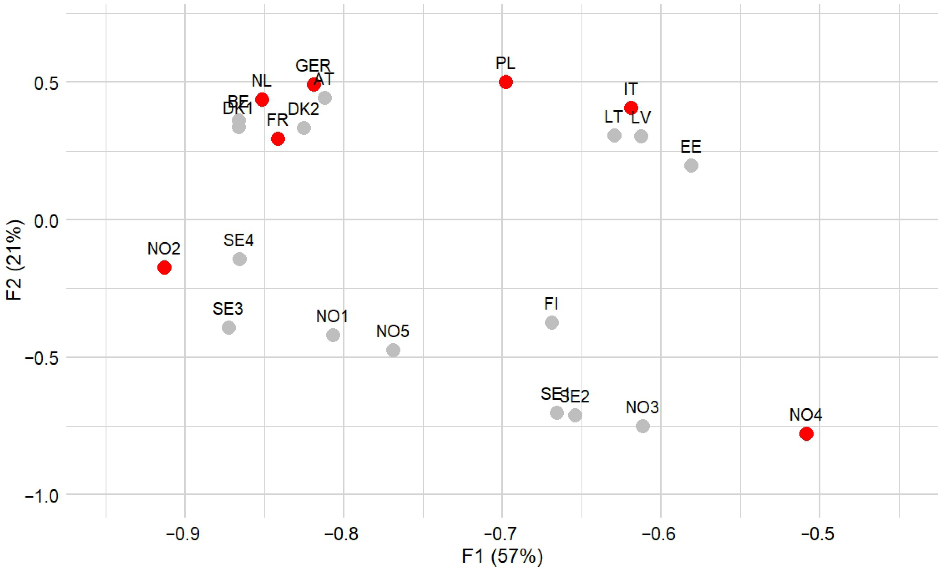
The main analysis was performed using ENTOS-E daily data for each of the 24 h of the two-year period 2023–2024 (731 days, 17,544 h). The initial selection of markets for the study was carried out taking into account the results of principal component analysis (PCA) of average weekly prices of electric energy published in the open access mode through the NORD POOL platform (https://www.nordpoolgroup.com/) for the two-year period of study (104 weeks).

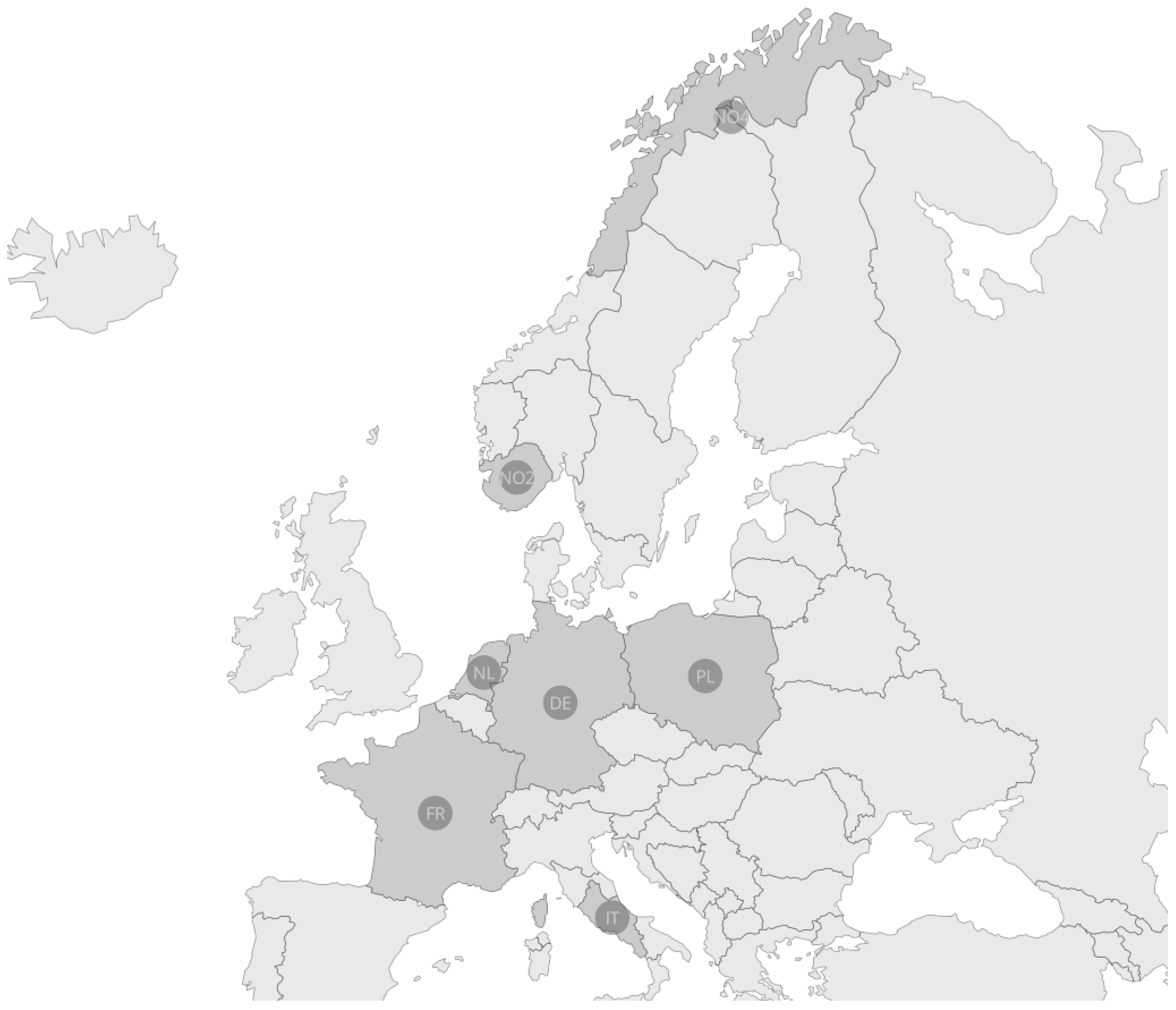
The selection of markets based on PCA was motivated by the need to reduce the number of optimal forecasting models to be identified, while ensuring that the chosen markets differed as much as possible in their electricity price characteristics. The PCA procedure has been described in the works [68,69]. Taking into account the distances between zones in the two PCA systems presented in Figure 2, which explain 78% of price variability during the study period, the following markets were selected for analysis: Poland (PL), Germany (DE), Netherlands (NL), France (FR), Italy (Center-South BZ denoted as IT) and two zones for Norway (NO2, NO4). For the IT market, aggregated weekly data published by the ENTSO-E Transparency Platform were used.

The geographical locations of the selected bidding zones are shown in Figure 3.

3.3. Energy Mix in Selected Bidding Zones

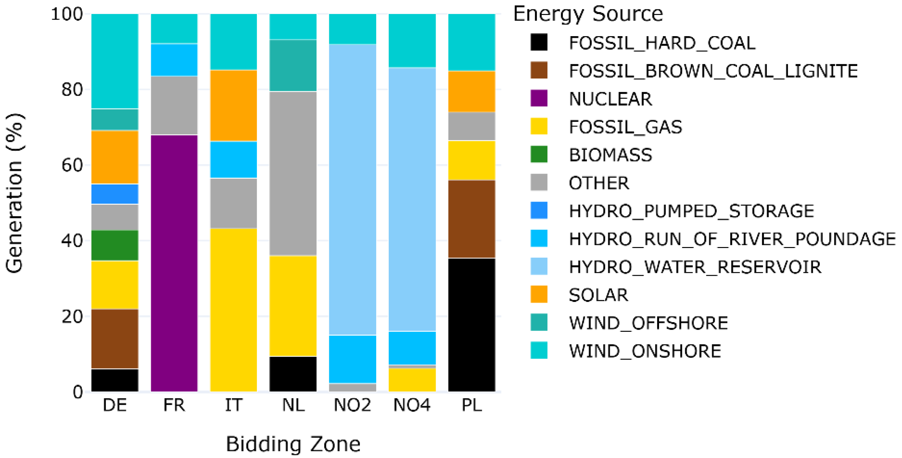
In addition to the statistical data, a concise overview of the energy mix in individual bidding zones is provided. At the national level, electricity is produced either through thermal generation—using heat from fuel combustion or nuclear reactions—or through RESs such as solar, wind, or hydropower. To illustrate the diversity of electricity generation across Europe, this study examines selected bidding zones, as shown in Figure 3 and discussed in the previous section.

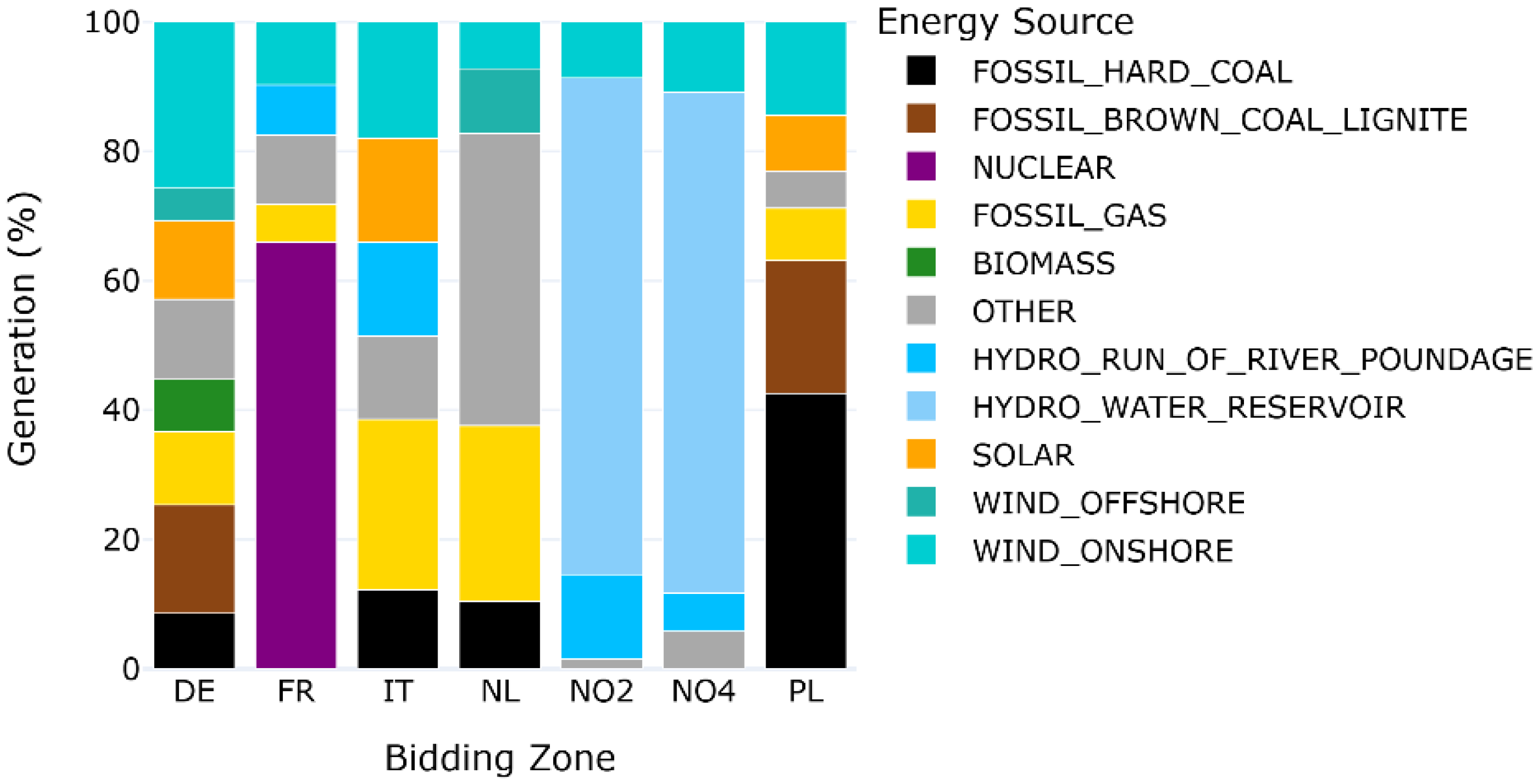
The variation in energy mixes (Figure 4 and Figure 5) reflects underlying differences in resource availability, policy frameworks, and decarbonization strategies.

Below, drawing on the collected data, as well as ENTSO-E reports [70,71] and the relevant literature [59], a brief characterization of the selected bidding zones is presented.

Germany is undergoing a major energy transition, aiming for 80% RESs by 2030 and 100% by 2035. The shutdown of its last nuclear reactors in 2023 marked a shift toward wind and solar, which now account for more than half of total generation. Coal’s share dropped from 37% in 2023 to 34% in 2024. Germany faces challenges in grid stability and dispatchable capacity, but continues to invest in infrastructure and flexibility.

In contrast, in France the energy mix is dominated by nuclear power, which accounted for 64% of electricity generation in 2023 and over two-thirds in 2024. This ensures a low-carbon baseload capacity but introduces risks related to aging infrastructure. Solar and wind contributed 12% in 2024, while fossil fuels made up just 3.5%. France remains the world’s largest net exporter of electricity due to low generation costs.

Meanwhile, Italy is divided into six bidding zones, shaped by geographical conditions. While solar and wind are increasingly integrated, fossil fuels remain significant, particularly in the Central-South zone, where gas use rose notably between 2023 and 2024.

Turning to the Netherlands, this country generated nearly half of its electricity from RESs in 2023, mainly from solar and wind. Fossil fuel use declined slightly in 2024, while conventional coal and gas plants are gradually being replaced. Decentralized and local generation is on the rise, supported by growing offshore wind capacity, which currently stands at 4.5 GW.

In the case of Norway, the country benefits from abundant hydropower, resulting in high electrification and low emissions. However, regional disparities and weather variability affect grid balance. To address this, the country is divided into five bidding zones (NO1–NO5). In this study, we focus on two distinct cases. Southern Norway (NO2) typically has surplus hydro generation and lower prices, while northern Norway (NO4) experiences higher prices due to limited transmission and reliance on weather-dependent RESs.

Finally, Poland continues to face transition challenges due to its reliance on coal. Nonetheless, recent years have seen growth in RESs and improvements in energy efficiency. While nuclear power is expected to play a future role, the current mix remains dominated by conventional sources.

In summary, the heterogeneity in energy mixes suggests differentiated resilience profiles and green energy transition pathways, with implications for cross-border electricity trade, system stability, and policy coordination within the European energy market.

3.4. Statistical Analysis of Selected Bidding Zones

This section provides a statistical analysis of the energy mix characteristics in selected European BZs. While the previous section offered a general introduction to the energy mix, as presented in Figure 4 and Figure 5, the focus here is on identifying key structural differences in electricity generation across regions, with particular attention to dominant sources and notable patterns. Examining these zones reveals how geography, resource availability, and market design shape national energy profiles. Understanding these regional characteristics is essential for analyzing electricity price volatility in the Pan-European market coordinated by ENTSO-E.

The statistical analysis of price distributions included cross-market comparisons, along with an examination of the relationships between prices and the explanatory variables used for forecasting. The empirical distribution parameters for hourly electricity prices over the study period are presented in

Table 1. Parameters of hourly price distributions [EUR/MWh] 2023–2024. The grey-shaded row represents the mean values across the respective bidding zones.

Parameters	DE	FR	IT	NL	NO2	NO4	PL
max	936.28	284.21	298.20	872.96	898.25	332.00	630.19
percentile0.9	138.28	135.28	165.00	137.30	108.88	52.02	153.23
percentile0.75	112.47	107.21	135.12	112.55	85.80	35.15	126.10
mean	86.83	77.41	118.07	86.54	64.77	26.64	103.94
median	88.91	80.41	113.12	89.65	59.31	22.47	101.95
percentile0.25	63.03	43.63	97.85	64.55	41.89	11.07	81.75
percentile0.1	15.63	8.91	82.00	16.98	23.86	3.06	57.59
min	−500.00	−134.94	0.00	−500.00	−61.84	−10.06	−61.64
R	1436.28	419.15	298.20	1372.96	960.09	342.06	691.83
IQR	49.44	63.59	37.27	48.00	43.91	24.08	44.35
sd	50.91	47.33	35.68	50.13	38.17	22.81	44.72
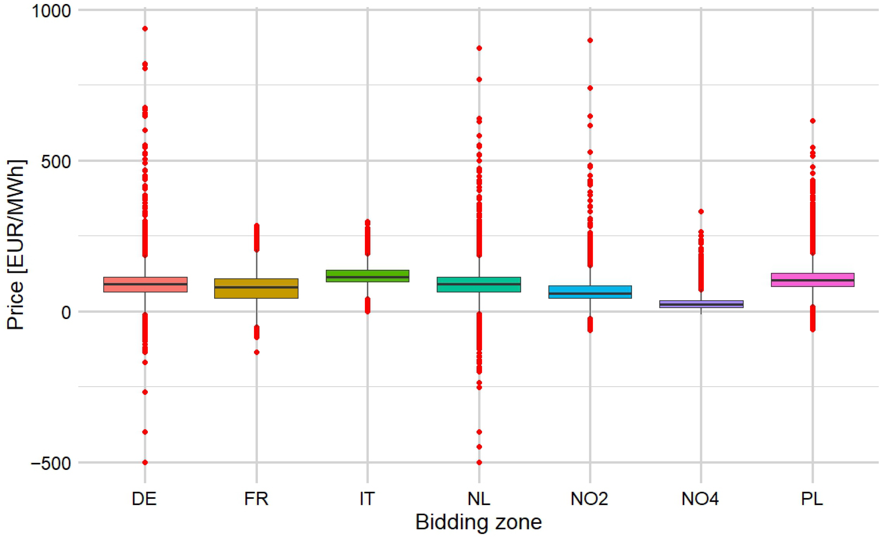
V [Index]	0.59	0.61	0.30	0.58	0.59	0.86	0.43

. The lowest average prices were observed in the NO4 zone, where over 90% of observations (the 90th percentile) do not exceed the average of remaining markets. This market also exhibits the highest relative price dispersion for the lowest prices. The highest average prices were observed for the IT and PL markets, while the highest prices were noted in the DE, NO2 and NL zones.

Average prices across the analyzed markets vary significantly (Table 1). The lowest average price, 26.64 EUR/MWh in the NO4 zone, is more than four times lower than the highest average price of 118.07 EUR/MWh recorded in IT zone. The average price in the PL area is similar to that in IT. In the DE, FR, and NL zones, very high average prices are also observed, exceeding the NO4 price by more than a factor of three. The NO2 zone is characterized by relatively lower prices compared to other markets, almost half the price in IT, but still more than twice the price in NO4. The highest price variability (i.e., R) is observed in the DE, NL, and NO2 markets, while the lowest variability is found in the IT zone, which has the highest average prices, and in NO4, which has the lowest. When excluding outliers, the highest interquartile range (IQR) is observed in FR. The highest average price variation during the investigated period was recorded in the DE and NL zones, while the lowest was observed in NO4 and IT. Relative to the average prices in each zone, the greatest variation occurred in NO4 (85.60%). Prices in FR, DE, NO2, and NL are characterized by relatively high volatility. The coefficient of variation is lowest in the IT and PL markets, yet still indicates significant price variability in these zones.

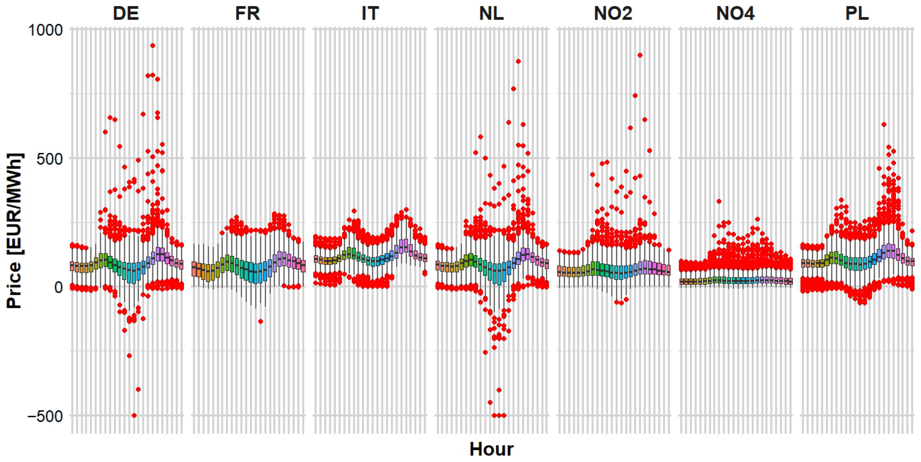
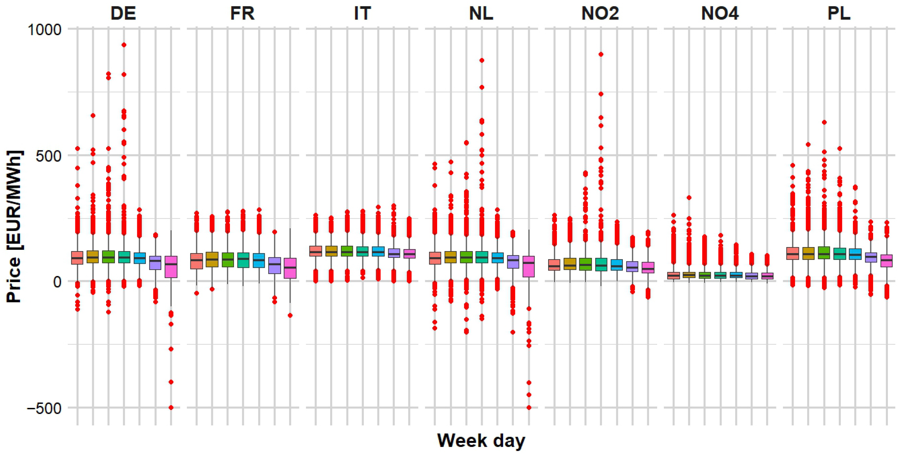
In Figure 6 hourly empirical distributions of prices are presented in the form of box-plots. For each market, high prices classified as outliers are observed. The highest extreme values were achieved for the DE, NO2, and NL markets. For most markets, negative outliers were also observed. The lowest extreme prices were observed in the DE and NL markets.

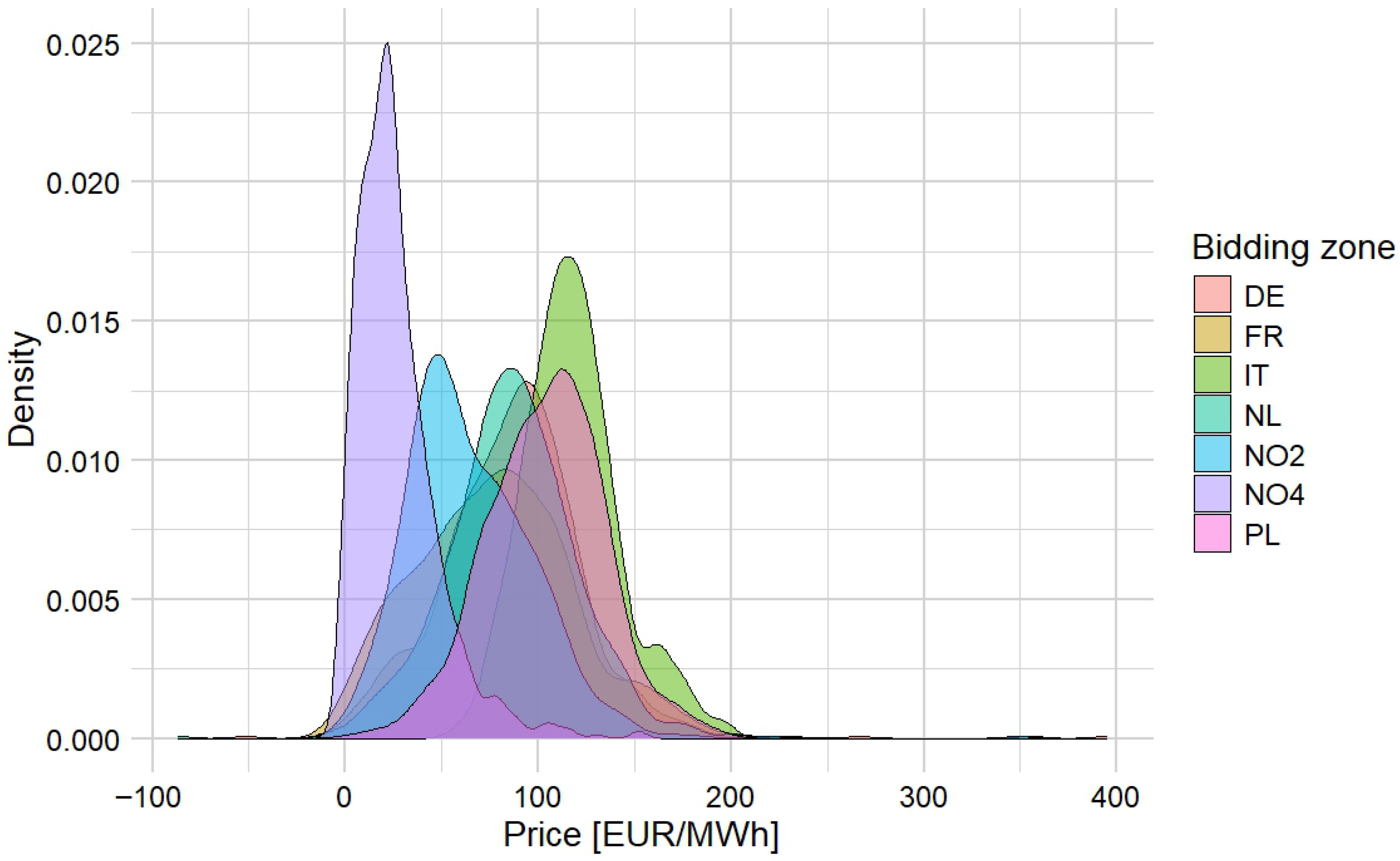
Hourly price distributions are characterized by substantial positive skew. The distribution of average daily prices is mostly positively skewed and substantially leptokurtic, as inferred from Figure 7.

The participants of the NO4 market are most likely to enjoy low prices. This market is characterized by a strong concentration of prices around expected values and substantial positive skew. For the neighboring NO2 market, prices are somewhat higher. Nevertheless we observe a higher price dispersion and less substantial positive skew. Price distributions for FR, NL and DE markets are similar in terms of average level and dispersion. For daily aggregation, negative skew was observed in FR and DE markets. The distribution of daily prices in the NL market is symmetric. For PL and IT zones, prices are concentrated at high levels. The skewness of the daily average distribution for the PL zone is close to that of DE and FR markets. The price distribution for the IT zone resembles that observed for NO4, but shifted upwards by 100 EUR/MWh.

The diversity of distributions and clearly visible deviations from a normal distribution justify the search for nonparametric prediction models.

Due to highly skewed distributions, and the presence of outliers, for modelling and forecasting of electricity prices in selected markets we decided to use nonparametric models. After preliminary selection, some of time series available at the ENTSO-E Transparency platform were used as explanatory variables. In

Table 2. Variables used in the study and their correlation with electric energy price.

Variable	Unit	DE	FR	IT	NL	NO2	NO4	PL
F(Load)	[MW]	0.26	0.39	0.38	0.40	0.33	0.45	0.13
F(Load-RES)	[MW]	0.79	0.54	0.62	0.57	0.43	0.58	0.36
F(Solar)	[MW]	−0.34	−0.27	−0.31	−0.33	×	×	−0.28
F(Wind off-shore)	[MW]	−0.32	−0.36	×	−0.29	×	×	×
F(Wind on-shore)	[MW]	−0.40	−0.23	−0.12	−0.32	−0.21	−0.20	−0.24
F(Total RES)	[MW]	−0.61	−0.40	−0.34	−0.49	−0.21	−0.20	−0.36
Day of a year	1:365 (366)	0.02	−0.07	0.05	0.01	−0.26	−0.27	−0.03
Hour	0:23	0.17	0.19	0.24	0.18	0.10	0.06	0.23
Month	1:12	0.02	−0.07	0.05	0.01	−0.25	−0.26	−0.04
Weekday	0:6	−0.21	−0.19	−0.14	−0.19	−0.14	−0.11	−0.24
Price $D-7$	[EUR/MWh]	0.48	0.67	0.75	0.55	0.52	0.51	0.60
Price $D-1$	[EUR/MWh]	0.65	0.79	0.80	0.66	0.74	0.81	0.70
Mean daily price $D-1$	[EUR/MWh]	0.48	0.71	0.59	0.47	0.71	0.82	0.45
Mean daily price $D-7$	[EUR/MWh]	0.27	0.55	0.54	0.31	0.48	0.50	0.34
Mean weekly price $D-1$	[EUR/MWh]	0.36	0.65	0.59	0.39	0.63	0.70	0.39

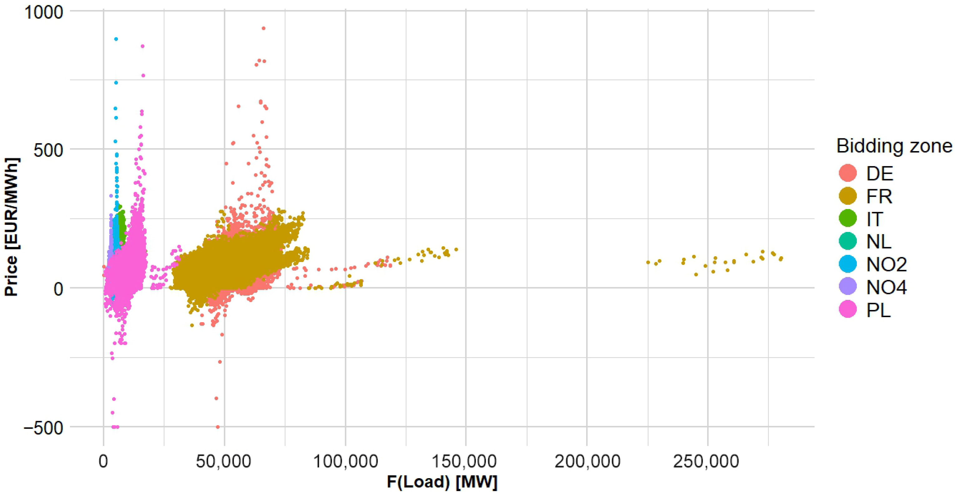
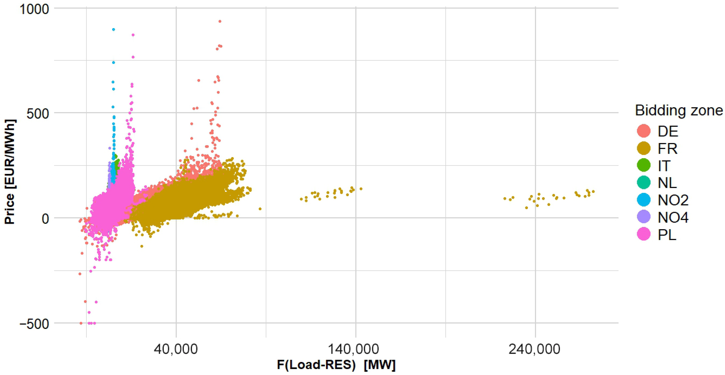
Notation used in the table: F(X)—forecast of the variable X for the day D from the previous day (day ahead forecast), D—current day, $D-1$—previous day, $D-7$—one week ago, ×—no data available

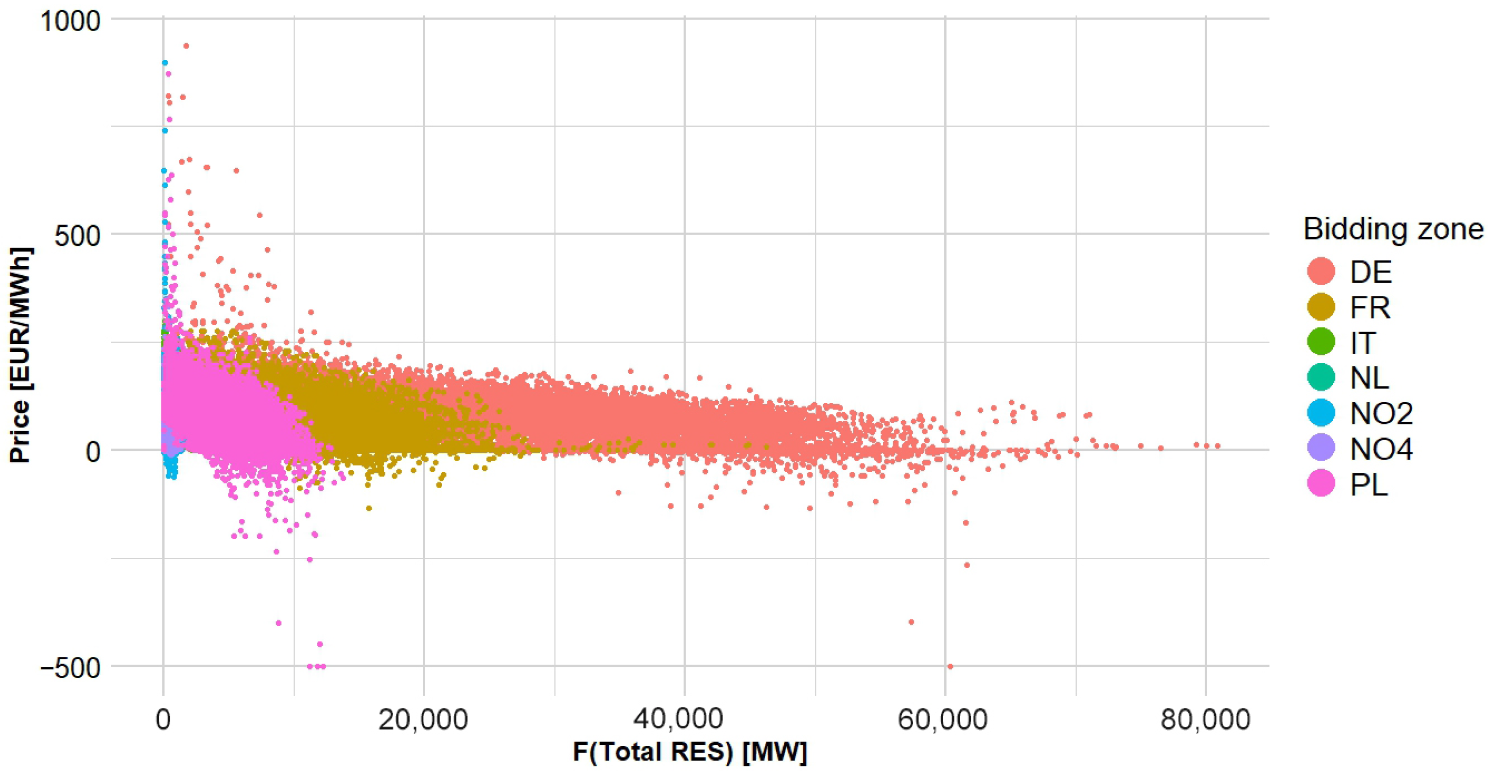
information on auxiliary variables used in models and their correlations with prices in respective markets is presented. Moderate positive dependencies are observed between the forecasted demand (F(Load)) and predicted generation without RESs, denoted as F(Load-RES). The analysis of scatter plots suggests that these dependencies are linear (Figure 8 and Figure 9). Mostly positive correlations are observed between the current price and the price (or average price) from one day and one week earlier. For each considered market, energy prices are negatively correlated with the amount of energy produced from renewable sources (F(Total RES)). They also seem to be linear (Figure 10). For variables related to time (Day of Year, Hour, Month, Weekday) dependencies are no longer linear (Figure 11, Figure 12 and Figure 13).

Correlation scatter plots for dependencies between a given variable and prices in every hour of the study period are presented in Figure 8, Figure 9 and Figure 10. Respective markets are denoted by different colors. Observed dependencies may be interpreted as linear. Nevertheless, Figure 8 and Figure 9 show that for sufficiently high demand (for each market this means a different level), and for sufficiently high production not covered by renewable sources, energy prices reach very high values. Relatively low demand (Figure 8), low production from conventional sources (Figure 9) and high production from renewable sources (Figure 10) are associated with low or even negative energy prices.

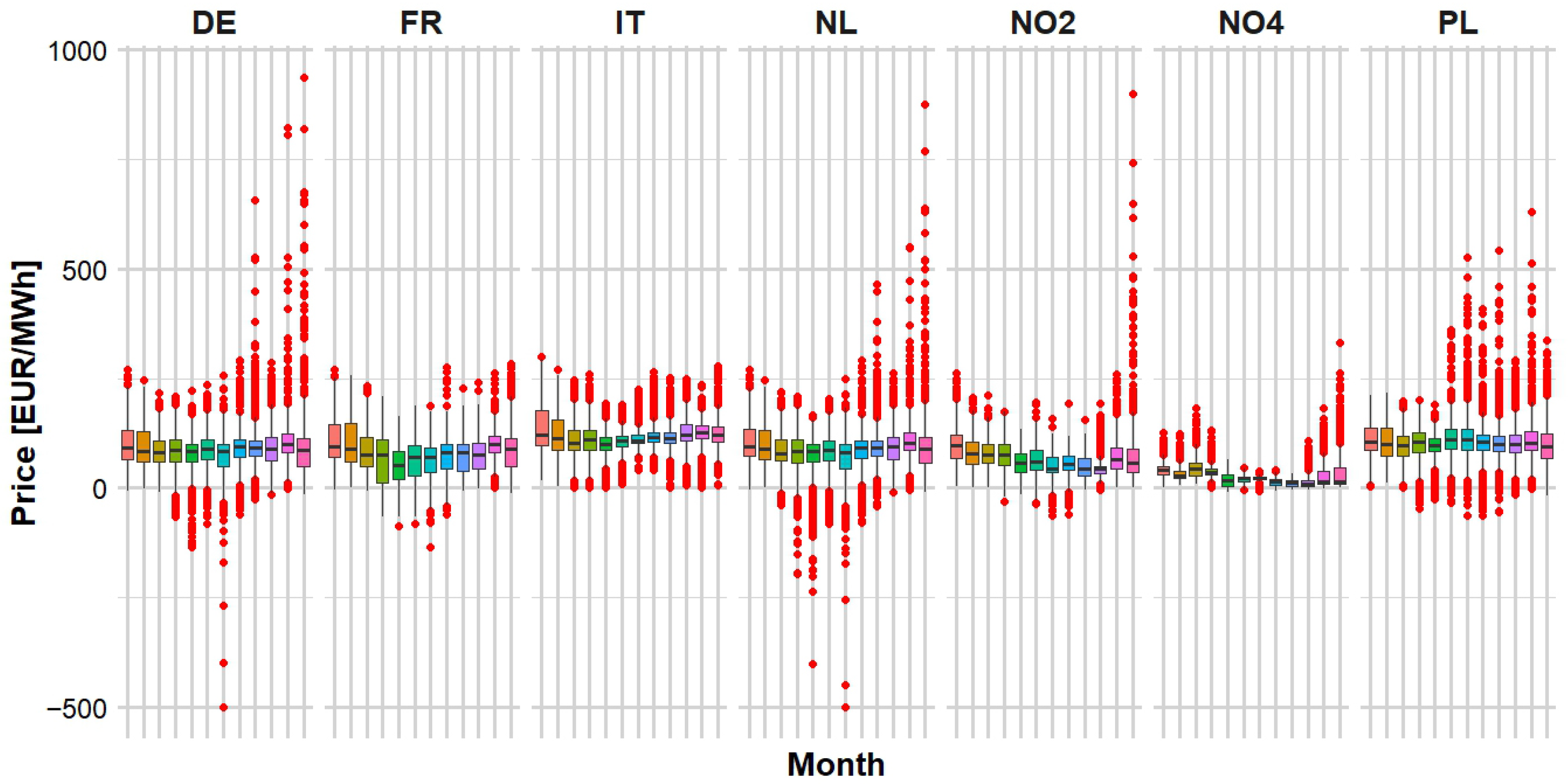
Figure 11, Figure 12 and Figure 13 present distributions of prices classified with respect to Hours, Months and Weekdays independently for each market. Each relevant time period has been distinguished by color, while outliers have been marked in red. The analysis of individual hours of the day (Figure 11) reveals higher price levels in the morning and evening peak hours. These are hours for which we observe gatherings of non-typically high prices. The effect is clearly visible for the DE, NL, NO2 and PL markets. In the middle of the day, low price levels dominate. In this period, for the DE and NL market, observed prices are substantially lower than typical prices. For the NO4 market, for every hour of the day, non-typically high positive values are observed. In the PL market both positive and negative outliers are also observed. For all analyzed markets, price distributions are characterized by positive skew and nonlinear dependencies on calendar variables.

For distributions aggregated by month (Figure 12), most markets exhibit relatively lower prices during the summer and higher prices during the winter. The behaviour of outliers follows the same pattern: atypically low prices occur predominantly in summer months, whereas atypically high prices are more frequent in winter.

When distributions are aggregated by day of the week (Figure 13), weekend prices tend to be relatively lower across most markets, particularly on Sundays. In this mode of aggregation, positive outliers are more likely to occur on working days, while negative outliers are more common on Sundays, especially in the DE and NL markets.

Based on this statistical analysis, the following is clear:

• Price distributions in individual zones are characterized by positive asymmetry and numerous outliers;
• Asymmetries in distributions are related to significantly higher atypical prices in the evenings and winter months;
• Atypically low prices tend to occur during midday hours in the summer and on weekends. These prices generally deviate less from the average level compared to the highest prices and are not consistently observed across all zones;
• The zones clearly differ in terms of price levels and the extent of their variability;
• The relationship between prices and demand and generation and RES generation is moderately linear;
• The current price is significantly correlated to prices from the previous day and the previous week;
• Price fluctuations over time exhibit nonlinear patterns.

3.5. Volatility Analysis

Key measures of volatility—range, interquartile range, standard deviation and the coefficient of variation—for the variables Intraday Price Range (IR), Absolute Daily Price Increase (AI) and Relative Daily Price Increase (RI) describing variability in seven of the considered zones between 2023 and 2024 (17,544 h, 731 days) are presented in

Table 3. Volatility measures.

Variable	Measure	DE	FR	IT	NL	NO2	NO4	PL
IR [EUR/MWh]	R	819.86	218.34	203.00	739.40	794.20	258.83	523.20
	IQR	64.46	47.05	47.57	65.80	37.94	15.28	55.14
	sd	66.02	31.83	34.28	62.74	43.51	20.32	68.60
	V*	0.63	0.40	0.41	0.57	0.91	1.17	0.72
AI [EUR/MWh]	R	1147.08	329.26	304.00	1078.75	1242.27	326.91	576.05
	IQR	33.93	28.26	17.85	31.39	17.04	8.27	29.27
	sd	42.37	30.78	22.58	41.08	27.56	13.96	34.32
RI [Index]	R	13.26	4.28	2.57	12.50	19.06	12.20	5.54
	IQR	0.39	0.37	0.15	0.36	0.27	0.31	0.28
	sd	0.49	0.40	0.19	0.48	0.42	0.52	0.33

V* is a non-dimensional value

.

In the study period the highest average price level and the lowest price variability were observed for the IT area (Table 1 and Table 3). In the Italian market we observe a modest price variability in the whole study period (V(P), Table 1), modest variability of within-day price ranges (IR, Table 3) and modest day-to-day changes (AI, RI Table 3). On average, relative rates of return deviate by +/−19% from the average week price (sd(RI), Table 3). But even in this stable market, the maximum volatility range reaches 257% (R(RI), Table 3).

The average price in the PL zone is somewhat lower than the price for IT (mean(P), Table 1), but we observed some high variability of price distributions and changes (V(P)—Table 1, day-to-day changes (sd(AI), sd(RI))—Table 3). Instead, we observe one of the largest intraday price variations here 72% (V*(IR), Table 3).

The lowest average price level was registered in the Norwegian NO4 zone (mean(P), Table 1), where the average price is over four times lower than that for the IT zone. For this market, prices fluctuated by +/−86% with respect to the average (V(P), Table 1). Daily relative variability with respect to the average reached 117% (V*(IR), Table 3). Average day-to-day changes were estimated at the level corresponding to 52% of the average weekly price (comparable to DE and NL; sd(IR), Table 3). The average absolute daily price change indicator classifies the area as stable with the lowest value of 13.96 EUR/MWh (sd(AI), Table 3).

The NO2 zone, with an average price more than double that of NO4, exhibits somewhat lower price variability (Table 1). Price distribution variability is similar to that observed for the DE, FR and NL markets (V(P), Table 1). Daily relative variability with respect to the average reached 91% (V*(IR), Table 3). Average daily price changes are at the level comparable to FR but lower than that of DE and NL (sd(RI), Table 3). Average absolute daily price changes are similar for the IT zone (sd(AI), Table 3). Wide ranges of daily return rates indicate the presence of outliers.

The DE and NL markets are similar with respect to price levels, price distribution parameters (Table 1) and variability measures within and between individual days (Table 3).

For the FR market, price ranges and variability measure ranges are narrower. This is due to the absence of extreme prices and extreme price changes within and between days. Price variability in the study period was estimated at 61% (V(P), Table 1, similarly to the DE, NL, NO2 markets). Within-day price variability is similar to the IT zone (IR, Table 3) and day-to-day change dynamics resemble those of NO2 (sd(AI), sd(RI), Table 3).

Given the diversity of energy price distributions across different markets, in this section of the article we compared price volatility in the studied zones both during the day and from day to day. Price volatility in individual markets is very high, both during the day and from day to day. In markets where there is high price diversity, we also observe large differences in price volatility over time. Exceptionally low diversity and volatility are observed in the IT zone, where energy prices are the highest. On the other hand, relatively high price volatility is observed in the NO4 zone.

Due to clearly asymmetrical price distributions in individual markets and non-linear relationships between study variables and prices, nonparametric models were used for prediction. Additionally, due to the dynamic volatility of the forecast values, the forecasts were determined adaptively in a moving diagnostic window one day ahead.

4. Forecasting Study

The next step in the study was to prepare predictive models. During the preliminary stage of our analysis, we evaluated a few different models.

ARIMA models were estimated using a moving-window approach for the German market. While the in-sample results were satisfactory, the out-of-sample performance proved inadequate. Specifically, for one-day-ahead forecasts, the RMSE exceeded 50 EUR/MWh. Given the magnitude of these forecast errors, the pronounced deviations from normality in the residuals, and the substantial computational time required for repeated re-estimation, we ultimately decided to exclude ARIMA from the set of models considered in the final study. Due to the substantial price volatility observed in the data, we also tested regime-switching models; however, they did not yield better results than the baseline models. Therefore, in the final stage of the study, we employed four canonical machine learning algorithms: Decision Tree Regressor (DTR), Random Forest Regressor (RF), Support Vector Regressor (SVR), and k-Nearest Neighbor (KNN) Regressor to obtain a day-ahead forecast of the price (for each hour).

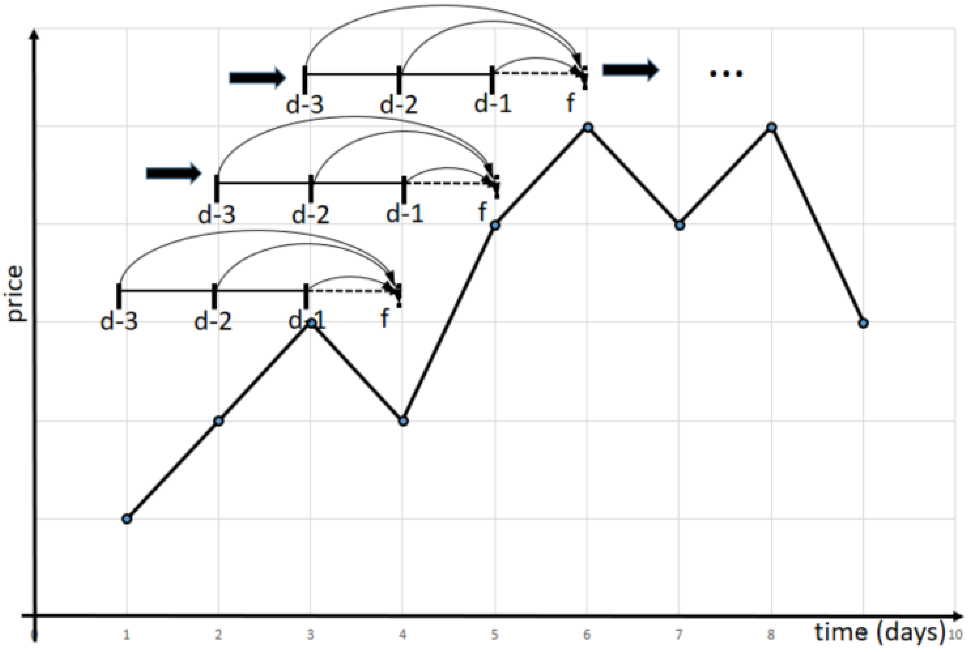
For each method, an identical learning mechanism was used, based on a sliding time window of variable length (see also [7,57] and compare Figure 14). Preliminary detailed calculations indicated that the relationship between forecast error and the length of the time window is generally smooth. Therefore, to accelerate computations during the full study, the analysis was conducted for selected values of the window length, using an increasing step size. The calculations were performed for windows with a length of $n=\{1,3,6,10,15,20,30,40,60,100\}$ days; i.e., the training set consisted of data from n days preceding the day for which the price was forecasted. Additionally, we used naive forecast as a benchmark for the considered algorithms.

The RMSE was adopted as the quality measure. This measure is based on absolute values and is the most commonly used measure of energy price forecast quality in the literature and in practice when focusing on a single market/bidding zone. However, due to the large differences in prices between bidding zones (see Table 1), the NMAE was chosen as a complementary measure, as it better shows relative differences and allows for comparison of the quality of forecasts obtained in different markets. More information on the advantages and disadvantages of individual measures in the selection can be found, among others, in [48,72].

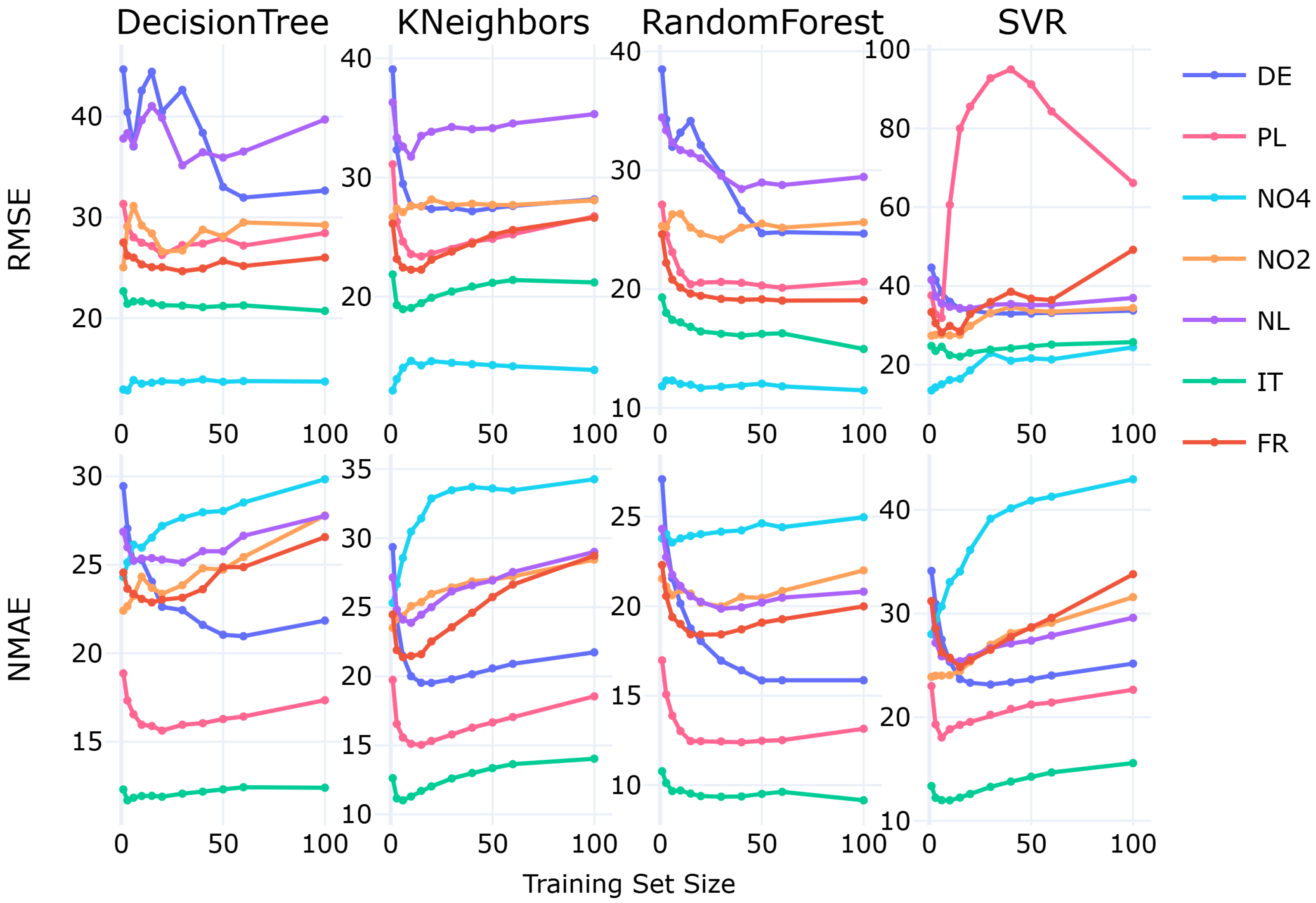
The results of the calculations are summarized in

Table 4. RMSE of forecasting for selected bidding zones.

Zone	DTR	Win. Size	KNN	Win. Size	RF	Win. Size	SVR	Win. Size	NAIVE
DE	31.95	60	27.18	40	24.67	100	32.97	50	42.01
FR	24.66	50	22.26	10	19.03	60	28.18	6	30.42
IT	20.72	100	18.95	6	14.96	100	22.05	15	22.55
NL	35.16	30	31.76	10	28.42	40	34.29	20	40.83
NO2	25.04	1	26.67	1	24.19	30	27.38	1	27.53
NO4	12.84	3	12.12	1	11.47	100	13.46	1	13.82
PL	26.28	20	23.37	15	20.11	60	31.87	6	34.22

and

Table 5. NMAE of forecasting for selected bidding zones.

Zone	DTR	Win. Size	KNN	Win. Size	RF	Win. Size	SVR	Win. Size	NAIVE
DE	20.96	60	19.52	20	15.85	60	23.15	30	31.04
FR	22.87	15	21.39	6	18.41	30	24.83	15	27.53
IT	11.69	3	11.02	6	9.15	100	11.98	10	12.35
NL	25.13	30	23.86	10	19.86	30	25.40	15	29.50
NO2	22.41	1	23.51	1	19.99	30	23.89	1	24.57
NO4	24.31	1	25.31	1	23.56	6	28.00	1	30.11
PL	15.63	20	15.04	15	12.40	40	18.04	6	22.04

and shown in Figure 15. For each zone and each regressor, the best-performing result is presented along with the corresponding time window length during which this result was achieved.

For all BZs, the best results for both RMSE and NMAE were obtained for RF (bolded values in tables Table 4 and Table 5).

The differences between RF forecasts and forecasts of other models are significant (at the 0.05 level) for the majority of models based on the Diebold–Mariano test (more information is provided in Appendix B) [73,74].

The results of the study also indicate a relationship between the level of market volatility and the length of the period from which training data should be taken. For highly volatile markets (NO2, NO4), in almost all situations, the best forecast results were obtained for models trained on short or very short periods preceding the forecast. For markets with lower price volatility (IT, DE, PL), the best results were obtained with larger time windows (longer training data history). The lower the price volatility, the more advantageous a longer training data period is. The results obtained therefore confirm the findings of the aforementioned studies [7,57].

5. Analysis and Discussion of Interdependencies Between Volatility, Energy Mix and Forecast Quality

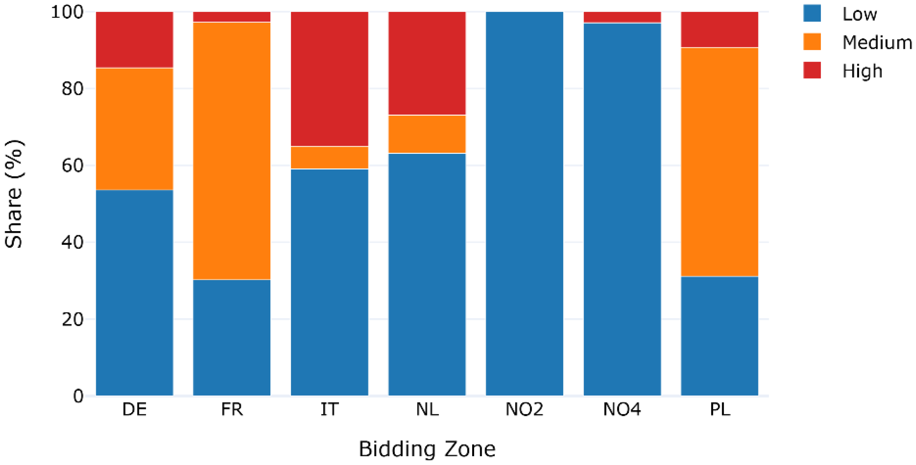
The next step is to examine the interdependence between price volatility in a specific market and the quality of the forecast. Based on ENTSO-E data, the total generation for each generation source and its share in total energy generation in 2023–2024 was calculated for each zone (

Table 6. Total generation (TWh), 2023–2024.

Bidding Zone	Low	Medium	High	Total
DE	488.18	289.83	132.89	910.90
FR	305.85	678.87	28.00	1012.72
IT	32.63	3.27	19.35	55.25
NL	143.89	22.61	61.29	227.79
NO2	105.75	0.00	0.00	105.75
NO4	50.06	0.00	1.48	51.54
PL	97.19	185.71	28.92	311.82

and Figure 16). Then, based on data from the literature and expert knowledge, each generation source was assigned to one of three flexibility categories (low, medium, high). In the final step, the strength of the relationship between the share of each flexibility category of sources and the magnitude of forecast errors was examined.

Although many publications have been devoted to the issues of the flexibility of the energy system as a whole and the flexibility of the sources themselves (see, for example, [75,76,77,78,79]), due to the multitude of factors influencing flexibility, the concept of generation source flexibility has not been clearly defined [79].

For the purposes of this study, it has been assumed that the flexibility of a source (also referred to as the availability of a source) is understood as the result of the speed at which a given source can deliver specific power and the ability to demand specific power at a specific time. The first value, referred to as the ramp rate, is expressed as a percentage of the amount by which a specific source can increase the power supplied per unit of time (usually per minute). The second feature is related to the degree of certainty that a specific source will be able to deliver a specific amount of power at a given time in the future (the ability to operate according to schedule). Taking both characteristics into account results in the following summary:

• Sources with low or zero flexibility include solar and wind sources (no predictability) and hydroelectric power plants (low ramp rate)—hereafter referred to as Low;
• Sources with moderate flexibility include hard coal and lignite power plants, biomass, and nuclear power plants (high predictability but lower ramp rate)—Medium;
• Sources with high flexibility include fossil gas power plants and hydro pumped storage (both a high ramp rate and predictability)—High.

Next, based on the results of analyses of the seven selected bidding zones in the period 2023–2024, we examined the relationships between the energy mix of individual characteristics, the level and volatility of electricity prices, and the quality of the forecasts obtained.

Table 7. Summary of indicators for individual zones.

Zone	Low	Medium	High	RMSE	NMAE	V(P)	V(IR)	Sd(AI)	Sd(RI)	Mean(P)
	[%]	[%]	[%]	[EUR/MWh]	[%]	[%]	[%]	[EUR/MWh]	[%]	[EUR/MWh]
DE	53.59	31.82	14.59	24.67	15.85	58.52	62.95	42.37	48.99	86.83
FR	30.20	67.03	2.77	19.03	18.41	61.04	39.78	30.78	39.97	77.41
IT	59.05	5.93	35.02	14.96	9.15	30.16	40.57	22.58	19.07	118.07
NL	63.17	9.92	26.91	28.42	19.86	57.82	56.76	41.08	47.60	86.54
NO2	100.00	0.00	0.00	24.19	19.99	58.96	91.33	27.56	42.28	64.77
NO4	97.13	0.00	2.87	11.47	23.56	85.67	116.65	13.96	52.09	26.64
PL	31.17	59.56	9.27	20.11	12.40	42.94	72.12	34.32	33.02	103.94

provides a summary of the distribution of shares across the respective energy source categories from Table 6, prediction errors of RF models (Table 4 and Table 5), variability and price level measurements (Table 1 and Table 3) for each analyzed bidding zone.

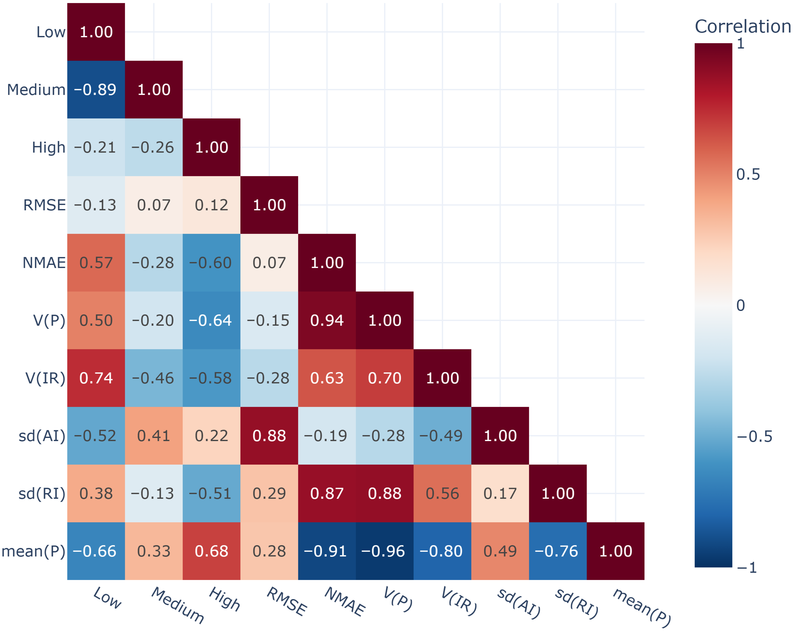
Based on the correlation matrix, Figure 17, dependencies between analyzed market characteristics were assessed.

Thus, we observed a moderate positive dependency between the increased share of (Low) generation and the variability and quality of forecasts expressed in NMAE. However, the calculations did not confirm this dependency measured in absolute error values (RMSE).

The results of the study also indicate a dependence between the level of market volatility and the length of the period from which training data should be taken. For highly volatile markets (NO2, NO4), in almost all situations, the best forecast results were obtained for very short periods of time. The lower the market volatility, the more advantageous a longer period of training data is.

Moderately strong dependencies between the share of (Low) in the general energy mix and remaining variables were observed. On the average, when the share of (Low) grows, lower average energy prices are observed (correlation coefficient: −0.66) and lower average day-to-day price changes (measured with the standard deviation of absolute price differences) are observed (correlation coefficient: −0.52).

No substantial dependencies between the share of (Low) and absolute prediction error measured by RMSE were detected.

However, moderate positive dependencies were observed between the share of (Low) in the general energy mix and relative measures of variability and prediction accuracy. On average, with the increase in the source share of (Low), we observe an increase in price variability (V(p), moderate dependency: 0.50), an increase in intraday variability (V(IR), substantial dependency: 0.74) and an increase in day-to-day variability (Sd(RI), weak dependency: 0.38). In addition, with the increase in the source share of (Low), we observe moderate growth in relative prediction errors measured with NMAE (correlation coefficient: 0.57).

No meaningful relation was observed between the share of sources with moderate/medium flexibility in the energy mix and remaining market characteristics.

For the share of sources with (High) flexibility in the energy mix, the observed dependencies are of comparable magnitude to those associated with (Low) flexibility, but exhibit opposite signs. Specifically, an increase in the (High) share is positively correlated with an increase in the average price (correlation coefficient: 0.68).

No statistically significant dependencies were identified between the (High) share and prediction errors evaluated using RMSE.

However, a moderate negative relationship was observed between the share of (High) and both relative price variability measures and prediction model performance assessed via NMAE. On average, an increase in the share of high-flexibility sources in the energy mix is associated with a reduction in price distribution variability (V(P), −0.64), intraday price variability (V(IR), −0.58), day-to-day price variability (sd(RI), −0.51), and prediction errors (NMAE, −0.60).

Absolute prediction errors measured by RMSE are most strongly correlated with absolute day-to-day price changes (sd(AI), correlation coefficient 0.88). Meanwhile, relative errors (NMAE) are most strongly related to the variability of the price distribution (V(P), 0.94).

6. Conclusions, Limitations and Future Directions

In this study, period absolute prediction errors for the considered models are not correlated with the shares of respective sources in the energy mix. Moreover, they are not related to price level or price variability. Here we observe a marked increase in errors for large day-to-day price variability.

A moderate dependency was observed between the quality of forecasts measured by a relative NMAE metric and shares of respective sources in the energy mix. Prediction quality was observed to deteriorate with the increasing share of renewable sources, while it improved with a higher proportion of highly flexible sources in the energy mix. NMAEs are most strongly related to the variability in price distributions and price levels.

The analysis shows that a higher share of RESs (Low) in production is associated with lower average electricity prices but also with higher price volatility. In contrast, markets with a larger share of controllable, flexible generation units (High) tend to have higher and more stable prices. Increased volatility related to the use of (Low) also leads to lower forecasting accuracy, while a greater share of flexible sources improves the quality of predictions.

The findings reported by Maciejowska [8] are broadly consistent with our results. In said analysis of price volatility using quantile regression models for the German market, the author observed that increases in wind and photovoltaic generation tend to reduce electricity prices. She also demonstrated that the effect of wind generation on volatility is demand-dependent: when demand is low, wind output increases price volatility, whereas under high-demand conditions it reduces volatility. Photovoltaic generation, by contrast, was found to stabilize price fluctuations, as measured by the IQR index. In the present study, renewable sources were considered jointly, as our focus lay primarily on their flexibility rather than their renewable character per se.

Similarly, Pavlík and Bereš [9] identified a positive relationship between RES generation and price volatility, as well as year-to-year changes in the predictive performance of statistical models across several European markets, namely Germany, France, the Czech Republic, Slovakia, Poland and Estonia, over the period 2015–2025. Their results further confirm that the correlation between hourly renewable output and electricity prices is distinctly negative in a number of these markets. In addition, they show that countries exhibiting higher demand-side flexibility or greater cross-border interconnection capacity tend to display weaker RES–price correlations and reduced volatility.

In general, the results of this study confirmed, on a broader scale, the observations formulated in the literature with regard to individual energy sources [8,9,21,22] and methodological guidelines for predictive modelling [23,24]. This study provides empirical evidence that price volatility is closely tied to the structure of the energy mix and has a direct impact on forecast accuracy, an issue of considerable relevance for effective market management. For system operators and energy market regulators, the findings underscore the necessity of adapting to a market environment in which volatility driven by the growing share of low-flexibility generation sources plays an increasingly prominent role. This shift calls for moving away from a stability paradigm grounded in fixed market relationships toward one centred on adaptability and flexibility. It further highlights the need for parallel investments in highly flexible generation resources capable of mitigating the variability of renewable output, thereby reducing the risks associated with system instability and enabling more reliable price forecasting.

The results also reveal that, in highly volatile markets, the most accurate forecasts are obtained using very short training periods, whereas in more stable markets, longer training windows perform better. Static predictive models thus lose credibility in unstable conditions. Consequently, the development of forecasting approaches that dynamically adjust both the temporal scope of the input data and the length of the training window becomes essential. For analysts, this implies the need to revise traditional forecasting practices and to maintain a process of continuous model updating.

The governance of Europe’s electricity markets is shaped by ENTSO-E’s system planning and adequacy assessments, ACER’s regulatory oversight and market monitoring, and the European Commission’s legislative initiatives under the Clean Energy Package, as reflected in their cornerstone publications [71,80,81,82,83].

Price volatility and its link to the energy mix are key for the above-mentioned European stakeholders. ENTSO-E coordinates transmission system operators to ensure secure grid operation and conducts studies like the European Resource Adequacy Assessment (ERAA) and the Ten-Year Network Development Plan (TYNDP). ERAA evaluates adequacy and flexibility needs over a 10-year horizon, while TYNDP focuses on infrastructure planning to support decarbonization and system stability. Both studies, mandated by the EU Clean Energy Package, examine how renewable penetration correlates with price variability and how infrastructure mitigates volatility.

The Bidding Zone Review (BZR) further addresses structural inefficiencies signalled by volatility, guiding ACER in market design decisions. High volatility often reflects congestion and limited flexibility, influencing zone splits or mergers. Persistent volatility undermines investor confidence and raises hedging costs, making it a critical metric for regulators. Finally, ACER’s Market Monitoring Reports assess EU market integration and functioning, where accurate price forecasting supports liquidity analysis, volatility assessment, and policy recommendations.

Insights drawn from this research can also inform other economies in several ways. First, the findings illustrate how variations in market structure and the share of flexible versus low-flexibility generation sources influence volatility and predictive model performance. Economies with similar characteristics, such as high penetration of renewable energy, interconnected markets, or variable demand, can use these results to anticipate challenges in electricity price forecasting. Second, the demonstrated effectiveness of adaptive machine learning models under varying volatility conditions offers guidance for designing forecasting approaches in other regions. Finally, the evidence on the importance of dynamic adjustment of training periods and data windows highlights generalizable strategies for improving forecast reliability in both mature and developing electricity markets.

In summary, studying price volatility and its dependence on the energy mix is important for policymakers and is scientifically interesting because it may influence decisions across all levels of the energy sector. For system operators, it ensures grid stability and operational security; for regulators, it supports efficient market design and policy alignment; for analysts, it drives the development of adaptive forecasting models; and for investors, it provides transparency on risks and hedging costs. Ultimately, these insights enable a more resilient, flexible, and well-integrated European energy market.