Article

DecPD: A Deconstructed Deep Learning Approach for Partial Discharge Pattern Recognition

Department of Automation, Zhejiang University of Technology, Hangzhou 310023, China
*
Author to whom correspondence should be addressed.
Energies 2025, 18(23), 6245; https://doi.org/10.3390/en18236245
Submission received: 3 November 2025 / Revised: 24 November 2025 / Accepted: 26 November 2025 / Published: 28 November 2025
(This article belongs to the Special Issue Application of Artificial Intelligence in Electrical Power Systems)

Abstract

Recently, partial discharge pattern recognition (PDPR) for transmission cables has garnered increasing attention due to the severe power outages, equipment damage, and even major safety incidents resulting from the failure of partial discharge (PD) detection. However, existing PD data samples usually suffer from highly similar features and unbalanced distribution. Determining how to precisely realize the PDPR has become a challenge. In this study, an effective PDPR approach is proposed based on a newly designed deconstructed PD (DecPD) model and a customized loss function for PDPR. Notably, the refined deep learning network captures the discriminative features in both temporal and spatial dimensions through a dual-channel learning architecture. Additionally, an adaptive focal loss function is designed, which introduces a peak factor to establish focusing parameters for PDPR, thereby addressing the class imbalance issues. A comprehensive experimental evaluation using real datasets generated on a physical platform is conducted to verify our proposed method. Compared to other existing methods, our DecPD approach demonstrates superior performance, achieving an overall accuracy of 96.65% in the presence of environment noise.

1. Introduction

Recognition of partial discharge (PD) in transmission cables is fundamental to ensuring the reliability of high-voltage (HV) power transmission systems. The insulation degradation caused by thermal, electrical, ambient, and mechanical stresses may lead to severe consequences, such as large-scale power system failures or even fires [1,2]. The detection and recognition of PD during its early stage is essential to ensure the safety of HV power systems [3]. However, simple binary classification PD tasks struggle to deal with the complex nature of PD scenarios, such as environmental noise and varying operational conditions [4]. Determining how to effectively deconstruct raw PD data samples to refine the categorization of highly similar PD is a critical pattern recognition task [5]. Moreover, due to grid data privacy concerns and the difficulty in capturing subtle PD signals, the inherent class imbalance between PD and non-PD samples is also a crucial challenge.
In order to effectively deconstruct and refine classification, experts traditionally select and extract features—such as statistical, fractal, and frequency features—based on the physical properties of the signals and the discharge mechanism [6,7], following signal denoising. These features are subsequently fed into traditional machine learning methods, including support vector machines, shallow artificial neural networks, and fuzzy set theory. Providing effective prior knowledge for the model is undoubtedly useful in deconstructing raw PD data samples, but traditional machine learning methods no longer have an advantage when handling high-dimensional, long-sequence PD data samples.
With the demonstrated advantages of deep learning (DL) in handling high-dimensional and large-scale data, the refined categorization of PD has attracted increasing research attention. Early applications of DL in PDPR primarily employed convolutional neural networks (CNNs) due to their strong capability in extracting spatial features. CNN-based models have shown excellent performance in distinguishing the main PD categories—surface discharges, internal discharges, and corona discharges [8]—and therefore remain a core component in modern PDPR frameworks [9,10]. As contemporary PD measurements typically contain a large number of sampling points to ensure waveform completeness, subsequent studies have incorporated long short-term memory (LSTM) networks to capture temporal dependencies in PD sequences. However, given the limited availability of PD data caused by privacy and acquisition constraints, traditional LSTM networks often suffer from low data utilization efficiency. To mitigate this issue, bidirectional LSTM (BiLSTM) models have been adopted, enabling temporal interpretation in both forward and backward directions and demonstrating improved robustness under environmental noise [11]. In this context, related studies began to combine the localized spatial feature extraction of CNNs with the temporal dependency modeling capabilities of LSTMs [12]. As a result, serial CNN–LSTM architectures gradually emerged as a representative paradigm in PD pattern recognition [13]. Building upon this foundation, CNN–BiLSTM extensions further enhanced temporal representation by incorporating bidirectional contextual information, thereby improving noise resilience and achieving higher diagnostic accuracy in various insulation–fault recognition tasks [14,15]. Beyond these serial designs, more general hybrid CNN–RNN frameworks have been explored, integrating convolutional modules with diverse recurrent units to capture multi-scale temporal dependencies [15,16]. Such hybrid architectures provide greater flexibility in modeling the heterogeneous, transient, and often nonstationary characteristics of PD signals, forming an important methodological backdrop for the present work.
Although the aforementioned models achieve strong performance in binary tasks or in identifying broad PD categories, the refined recognition of highly similar PD types remains challenging. Addressing this problem requires models capable of effectively deconstructing long-duration samples, capturing short transient pulses, and processing high-dimensional PD data with improved feature discriminability.
In addressing the class imbalance issue in PDPR, it is essential to design a method with a small parameter size and high effectiveness to assist the aforementioned models [17]. Traditional approaches typically involve sampling techniques, such as the synthetic minority over-sampling technique, to artificially balance the dataset before model training [18]. When scarce samples cannot meet over-sampling conditions, data augmentation techniques are considered to improve the class imbalance of the dataset, such as using Wasserstein dual discriminator generative adversarial network to generate data for balancing the imbalanced samples [19] or employing information distillation to augment PD data [20]. Unlike the above methods, the authors of [21] proposed a reconstruction of the cross-entropy loss function, based on the standard cross-entropy loss, to address the issue of class imbalance. This method does not rely on over-sampling conditions and can ensure the integrity of the original dataset. However, this method requires complex parameter adjustments and has not yet established hyper-parameters tailored for PDPR.
Considering the growing demands of power transmission and the increasingly refined recognition requirements for PDPR, this paper proposes an effective PDPR method based on the deconstruct PD (DecPD) model. To address the challenge of PDPR under environmental noise, inspired by the ability of CNN and BiLSTM to capture temporal-spatial features of PD signals, a parallel architecture is proposed to first deconstruct the structural features from long-sequence PD data sample. Additionally, the design of the gated recurrent unit attention (GRAttention) module not only decomposes the features of short transient pulses but also allocates attention to PD time slices. The entire network model progressively deconstructs the original PD sequence, capturing discriminative features across long sequences, short transients, and multi-dimensional PD signals. Building upon this, to solve the issue of imbalanced sample class distribution, an adaptive focal loss (FL) for the PD scenarios is introduced, which improves the FL function to reduce computational resource consumption. The main contributions of this paper can be summarized as follows.
1.
For high-accuracy PDPR tasks, a refined PDPR network model based on DecPD is developed for PD samples under environmental noise. By incorporating parallel CNN-BiLSTM processing and the GRAttention module, the model effectively captures both long-term dependencies and short-transient PD features, enabling accurate discrimination among highly similar PD phenomena and significantly enhancing multi-type recognition performance.
2.
An adaptive loss function tailored for PD scenarios is proposed to address the severe class imbalance between non-PD and PD fault samples. By introducing a peak factor as an adaptive modulation term, the loss function eliminates the need for manual parameter tuning while preserving the ability to focus on sparse and difficult samples, thereby improving training efficiency and classification robustness.
3.
A real-world dataset generated from a PD data generation and acquisition platform is constructed to validate the proposed approach. The dataset contains seven PD categories measured under practical noise conditions, enabling comprehensive evaluation and demonstrating the effectiveness of the proposed method in realistic on-site environments.
The remainder of this paper is organized as follows: A detailed description of the proposed PDPR method is provided in Section 2, along with the data preprocessing process. Section 3 introduces the measurement equipment used to collect PD data with typical defects, validates the effectiveness of the proposed method, and compares it with other approaches. Finally, Section 4 presents the conclusions.

2. Proposed DecPD with Adaptive FL for PDPR

2.1. Overall Scheme

A block diagram of the proposed DecPD with the adaptive FL recognition framework is shown in Figure 1, which mainly consists of four parts. The first part pre-processes the PD dataset by Butterworth filter to filtering partial environmental noise and then splits it into time slices to reduce dimensionality. After the construction of feature matrix, the third part provides a detailed explanation of the structure and parameters of DecPD network model. Finally, Section 2.5 introduces adaptive FL for addressing the class imbalance issue.
To provide a clearer representation of the processing workflow, the three major stages-data preprocessing, feature extraction, and pattern recognition-are further decomposed as follows.
Step 1: Data Preprocessing
The raw PD signals with an original sequence length of 120,000 are first collected and then processed using a Butterworth filter to suppress high-frequency noise and determine the effective frequency band. After filtering, the signals are segmented into time slices of 400 sample points to reduce the sequence length and facilitate subsequent analysis.
Step 2: Feature Extraction
For each time slice, 32-dimensional time-domain features are extracted to characterize the temporal properties of the PD signals. In parallel, a Fast Fourier Transform (FFT) is performed to obtain 4-dimensional frequency-domain features, capturing the spectral characteristics of each slice. The time-domain and frequency-domain descriptors are then concatenated to construct a 36-dimensional feature matrix, providing a comprehensive representation of both temporal and spectral information.
Step 3: Pattern Recognition
Prior to training, the parameters of the DecPD model are initialized. The feature matrix is simultaneously processed by a 4-layer CNN, which extracts spatial representations, and a 2-layer BiLSTM, which captures long-range temporal dependencies. The outputs of both branches are fused and further refined using the GRAttention module to emphasize informative patterns. An adaptive focal loss function is applied during training to mitigate class imbalance and guide parameter updates. Finally, the fused features are fed into DenseNet for classification, and the model is iteratively trained until convergence or until a predefined accuracy or epoch limit is reached.

2.2. Data Preparation

It is widely recognized that raw signals from real transmission cables contain PD phenomena and environmental noise. While the discrete wavelet transform (DWT) denoising algorithm is commonly applied in related PDPR works and Kaggle competitions, it typically requires repeated parameter adjustments to achieve optimal performance [22]. In contrast, in the proposed method, only a Butterworth filter [23] is employed, which is chosen for its smooth frequency response, linear phase characteristics in the passband, and simple design. These properties allow effective suppression of high-frequency noise while preserving essential PD signal characteristics, including the sharp rise and exponential decay of pulses. Moreover, the cutoff frequency is dynamically determined based on the maximum and minimum amplitudes of the signal spectrum, enabling adaptive filtering of PD events without manual parameter tuning. This approach provides a practical and computationally efficient alternative to DWT, achieving comparable denoising performance while maintaining signal integrity, as detailed below.
X ^ PD = 1 1 + f [ k ] f 0 2 n X PD
where X PD is the input PD sequence, X ^ PD is the output signal after being processed by the Butterworth filter, n is the order of the filter, f 0 is the cutoff frequency range, and f [ k ] is the frequency value corresponding to the k-th frequency component, i.e.,
f [ k ] = k · f s N l
where N l represents the signal length, f s is the sampling rate.
To dynamically select the cutoff frequency range, and f main and f secondary are defined based on the highest and lowest amplitudes with
f main = f [ arg max ( | X [ k ] | ) ] ,
f secondary = f [ arg min ( | X [ k ] | ) ] .
Then, the frequency range is set as [ f 1 , f 2 ] with
f 1 = f main δ f main ,
f 2 = f sec ondary + δ f main .
where δ is the threshold ratio which is used to adjust the filter bandwidth.
Due to the transient nature of PD phenomena, numerous sampling points are typically required within short time intervals to ensure that each momentary PD event is captured [24]. To reduce computational load, the filtered dataset of 5668 PD samples is divided into time slices of 400 sampling points, resulting in a total of 300 slices per sample (each sample contains 120,000 sampling points).
The 400-point slice length was selected based on the typical temporal extent of a PD pulse, which generally spans only a few hundred sampling points. This window ensures that the entire pulse, including its rapid rise and exponential decay tail, is fully preserved without truncation. In preliminary evaluations, alternative slice lengths (200, 600, and 800 points) were also tested. Shorter slices (e.g., 200 points) occasionally truncated the decay component, whereas longer slices (e.g., 600 or 800 points) introduced redundant background data without improving feature representation. Therefore, the 400-point segmentation provides an effective balance between signal completeness, noise suppression, and computational efficiency. These slices are subsequently concatenated to capture the essential signal features [25].
Remark 1.
Based on the frequency range adaptively obtained by the Butterworth filter, PD signal filtering can be achieved with a simple and effective design. The minimum amplitude corresponds to the normal background frequencies during moments without PD and noise, while the maximum amplitude reflects the abnormal frequencies associated with PD events. Compared with DWT, this approach preserves the temporal characteristics of PD pulses, avoids extensive parameter tuning, and achieves comparable or superior classification performance.

2.3. Feature Extraction

Based on efficient features used in existing similar works, the following 32 time-domain statistical features are referenced; average voltage, maximum absolute voltage (by flipping all negative voltage PD peaks), standard deviation of voltage, voltage peak factor, voltage waveform skewness, voltage waveform kurtosis [26], voltage quantiles at 0%, 1%, 25%, 50%, 75%, 99%, 100% [26], and relative percentage quantiles (calculated as the percentage quantiles minus the average) [27], average peak pulse voltage width, maximum width, minimum width [28], average peak pulse voltage prominence, maximum prominence, and minimum prominence [29].
The prominence feature quantifies the extent to which a peak stands out from its surrounding signal environment and is widely employed as a robust descriptor for peak characterization under noisy conditions. It is formally defined as
prominence ( p ) = y ( p ) max ( L , R )
where y ( p ) denotes the height of the peak, L is the amplitude of the local minimum on the left side of the peak, and R is the amplitude of the local minimum on the right side. The term max ( L , R ) represents the higher of the two bounding minima that determine the effective baseline of the peak.
Then, the samples are processed using FFT [30], as given by
X ^ PD k = n = 0 N p 1 X ^ PD n · e j 2 π N p k n
where X ^ PD k is the k-th frequency component in the frequency domain, X ^ PD n is the n-th sample point in the time domain, and N p is the total number of sample points.
After performing FFT, four frequency-domain features are extracted from the power spectral density (PSD) [31], including the voltage PSD peak, PSD mean, PSD energy, and PSD entropy. The PSD is computed using Welch’s method implemented in SciPy, which employs the 256-point Hann window with 50% overlap to provide a smoothed and low-variance spectral estimate. The calculation of the PSD P i x is shown as follows by
P i x = 1 U N w k = 0 k 1 | X ^ PD k | 2
where k is the number of signal segments or windows used to smooth the power spectral estimate, N w is the number of sample points in each window, and U is the window normalization factor.
The energy and entropy of the PSD are defined as
P energy = i = 1 N P i x
P entropy = i = 1 N P i x · log 2 ( P i x + 1 × 1 0 10 )
Finally, the time-domain and frequency-domain features are concatenated into a 36-dimensional feature matrix, which serves as the input for the PDPR method. After feature extraction from the time slices, the PD samples are transformed into a feature matrix of length 300, reducing the learning parameter size without altering the original temporal-spatial feature, with each sequence corresponding to a time slice of the original signal.

2.4. Architecture of Proposed DecPD Model

The DL architecture can learn more discriminative features from the input data, which not only enhances recognition performance but also maintains robustness to environmental noise [32,33].
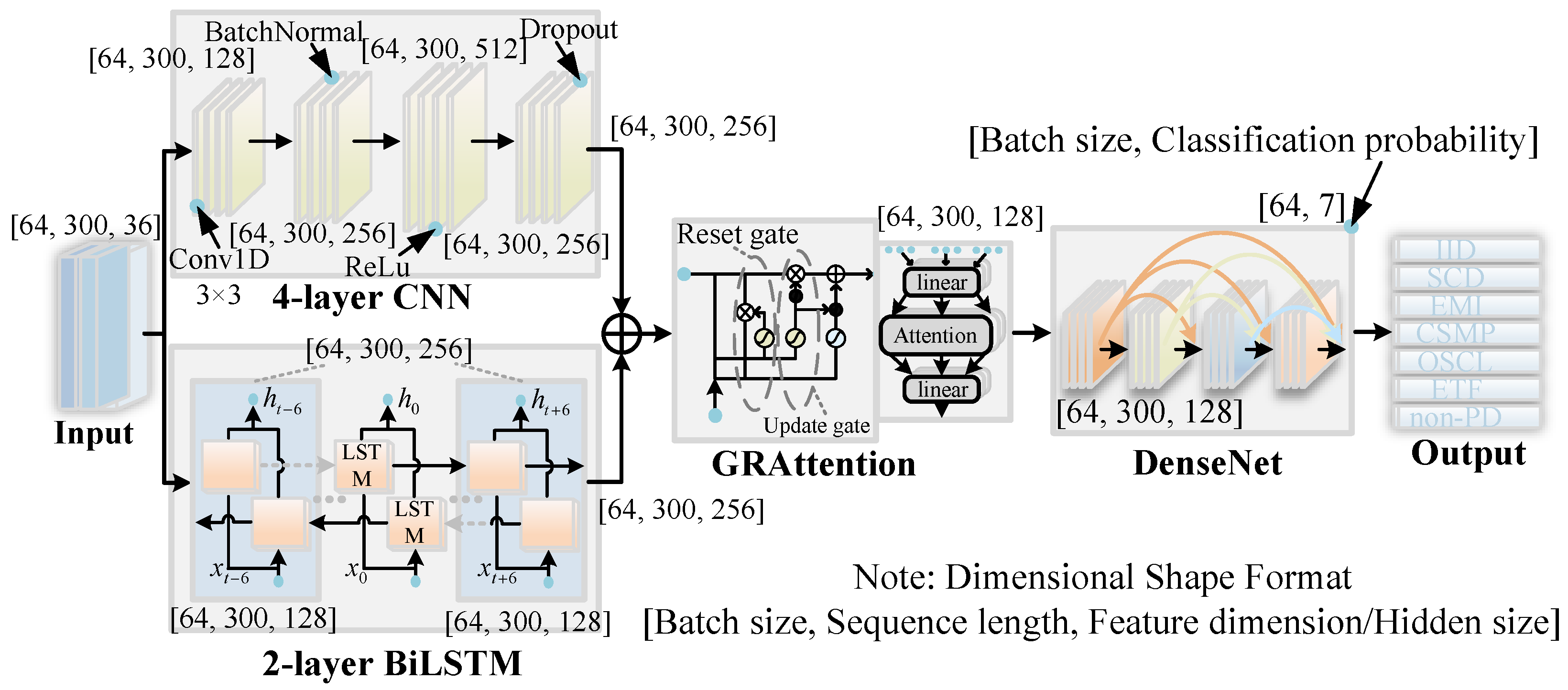
A refined DL network model based on DecPD is proposed to better distinguish PD defect types, as illustrated in Figure 2. The method consists of three key components, including (1) Dual-channel learning architecture, (2) GRAttention, and (3) DenseNet classifier.
The PD sequence is initially processed in parallel by 1D-CNN and BiLSTM. Specifically, after feature extraction from the input signal, the same features are simultaneously fed into both the CNN and BiLSTM branches. The CNN captures local spatial patterns, while the BiLSTM models long-term temporal dependencies. The outputs of the two branches are then combined via element-wise addition to form the overall feature representation, which is subsequently passed to the GRAttention module for capturing short-term dependencies before classification.

2.4.1. Dual-Channel Learning Architecture

A dual-channel learning architecture, inheriting the merits of both CNN and BiLSTM, is proposed to more effectively capture discriminative features. After initial feature extraction, the same input features are fed simultaneously into both channels in parallel. In the CNN branch, local spatial features are extracted from the feature matrix, mapping them into a new feature representation field through local connections with sliding window processing. This process identifies the spatial relationships between adjacent time slices and gradually deconstructs features with high spatial coherence and uniform structure [12]. Meanwhile, the BiLSTM branch leverages cell memory to capture long-term dependencies and dynamic sequential features in both forward and backward directions, effectively recognizing PD pulse patterns across the entire sequence, including both ends [11]. The outputs of the two channels are subsequently combined (e.g., via element-wise addition) to form a unified feature representation, which is then input into the GRAttention module for capturing short-term dependencies before classification.

2.4.2. GRAttention

Although the parallel architecture effectively deconstructs temporal-spatial features, capturing short-duration transient pulses is equally crucial for PDPR, as PD phenomena may recur within short time intervals in the overall PD sequence. To capture short-term dependency features, the gated recurrent unit (GRU) is selected for its simple structure and effectiveness. It performs a new round of temporal learning on the combined inputs [34].
At this stage, all time slices contain high-dimensional feature information, and directly feeding them into the classifier will lead to slow convergence, which motivates us to apply the GRAttention mechanism. After temporal learning, a multi-head attention mechanism is introduced to adjust the weight of each head based on the response degree of different time slices [35], with an emphasis on the time slices containing PD phenomena.

2.4.3. DenseNet Classifier

In the DenseNet classifier, each dense block consists of multiple convolutional blocks, with each convolutional block densely connected to all preceding blocks’ outputs [36]. Overall, DenseNet achieves feature reuse through the stacking of dense blocks and transition layers, optimizing network parameters and providing an efficient deep learning architecture for classification tasks.
Remark 2.
The dual-channel learning architecture of the DecPD model preserves the key role of CNNs in PDPR while addressing information gaps in the temporal aspect. Different from similar works, DecPD is designed based on the characteristics of PD data-long sequences, short transients, and multi dimensionality-resulting in a refined DL network. To further reduce the model’s parameter size, attention is focused on the time slices where PD occurs. The overall network model fully deconstructs the complex and redundant raw PD sequence samples, thereby enhancing its generalization performance across various PDPR tasks.

2.5. Adaptive Focal Loss

Due to the class imbalance between non-PD samples and PD samples, this may lead to gradient disparities during the training phase [37]. From the perspective of the loss function, a common approach to address gradient imbalance is cost-sensitive learning, which adjusts the classification balance without increasing computational complexity.
The work in [21] adds different weights to hard-to-classify and easy-to-classify samples in the cross-entropy loss function, reducing the weight assigned to well-classified samples. FL focuses on sparse difficult examples, preventing a large number of negative samples from overwhelming the detector during training.
The traditional multi-class FL function is defined as follows
FL ( p i , c ) = 1 N s i = 1 N s c = 1 C α c ( 1 p i , c ) γ log ( p i , c )
where N s is the number of samples, C is the number of classes, p i , c is the predicted probability for the i-th sample belonging to class c, α c is the balancing factor, and γ is the adjustable focusing parameter.
To find specialized parameters suitable for PDPR and reduce parameter tuning time, the two hyper-parameters α c and γ are adaptively designed, with their values determined by f c and p a r .
The value of α c is selected based on the sample class frequency f c , i.e.,
α c = 1 f c
Since some key information of PD signal is often concentrated at the pulse peaks of the sequence, the peak factor can characterize the degree of signal variation. The peak factor is typically expressed as
par = max ( x PD v ) RMS ( x PD v )
where x PD v represents the PD voltage amplitude, and RMS ( x PD v ) is the root mean square of x PD v .
For non-stationary signals (such as PD), the standard deviation σ PD better reflects the overall fluctuation of the signal. Therefore, the peak factor is slightly adjusted, and both peak and valley values are considered.
An improved adjustable focusing parameter γ is characterized by the average peak factor of the entire sequence
p a r = m a x ( | x PD v | ) 2 σ PD
γ = m e a n ( p a r ) + α
where p a r is the peak factor of the PD sample sequence, σ PD is the overall standard deviation of the PD sequence, and α [ 0 , 1 ] is the hyper-parameter to be adjusted.
Remark 3.
The improved multi-class FL addresses the class imbalance issue in the PD scenarios and eliminates the need for repetitive hyper-parameter tuning and cross-validation in traditional FL, resulting in a loss function specifically designed for handling class imbalance in PDPR.

3. Experimental Validation

In this section, a PD data generation platform is established to collect PD samples from six typical defect types and non-PD samples, constructing a dataset for the PDPR task. The experimental setup is then described in detail, followed by a comparison of denoising effects. Subsequently, an in-depth analysis is conducted on the effectiveness of the proposed method, specifically focusing on the DecPD model and adaptive FL tailored for the PD scenarios. Finally, the presentation of the experimental results and a comprehensive comparison with similar techniques confirm the advantages of the proposed method. The codes used in this section are all available online: https://github.com/ycWu-PD/DecPD (accessed on 1 November 2025).

3.1. PD Data Collection

3.1.1. Artificial Defect Description

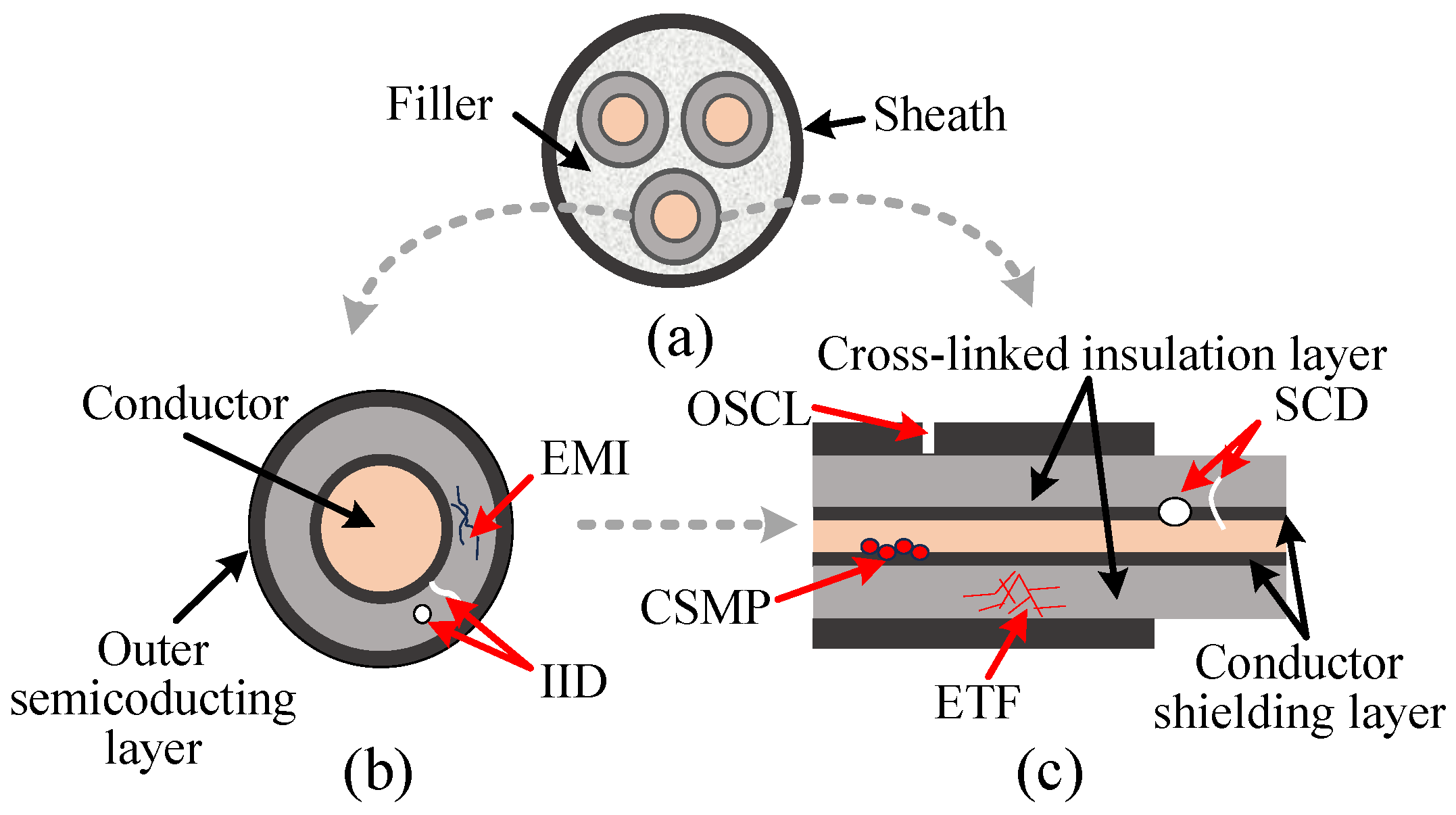
Six typical PD defects that are likely to occur under real-world conditions [29,38,39] are illustrated in Figure 3.
  • IID: Internal cracks or voids defects within cross-linked insulation.
  • SCD: Surface cracks or gaps on conductors causing conductor defects.
  • EMI: Embedded metallic particles within insulation causing conductive inclusions.
  • CSMP: Conductor surfaces with metallic particles exhibit defects under alternating electric fields.
  • OSCL: Outer cracks in semi-conductive layer causing insulation surface defects.
  • ETF: Internal insulation degradation causing defects via electrical treeing.
Two types of artificial environmental noise, i.e., white noise from the power grid and power electronic interference (PEI), were applied to the HV transmission cable to simulate the inherent noise disturbance encountered during real PD occurrences. The white noise generally refers to various types of random noise, such as coil thermal noise, ground network noise, and others. The PEI refers to pulse clusters with equal amplitude, the interfering pulses move in a directional manner along the phase baseline. Directly collecting PD data under environmental noise makes the data more representative of real-world PD occurrences in HV transmission cables, but it simultaneously increases the difficulty for subsequent PDPR.

3.1.2. PD Data Acquisition

The PD data generation platform was constructed in accordance with IEC 60270 standards [40], as shown in Figure 4. It mainly consists of a 7-m cross-linked polyethylene (XLPE) cable, a high-frequency current transformer (HFCT) for PD current detection, a wide-band digital oscilloscope (100 MS/s) for signal acquisition, and a PD generation device used to inject both defect signals and environmental noise [41].
The PD generation device transmits six types of PD signals via port A and two types of environmental noise via port B, which are injected into the XLPE cable through coupling electrodes. These coupling electrodes are distributed across the cable body, the cable joints, and the cable terminations, and their positions are alternated during testing to acquire PD signals from multiple locations. This setup enables the experiment to simulate the occurrence and propagation of internal, surface, and external discharge phenomena in actual operating cable systems, thereby improving the representativeness of the collected data. Port C provides a 50 Hz synchronization phase, which is fed into an oscilloscope together with the PD signals captured by the HFCT (deployed on the grounding strip of the transmission cable) [42]. The oscilloscope is configured with a data acquisition rate of 100 MS/s. For remote control, port D is connected to the control terminal via a wireless bridge. The synchronization phase signal can be reliably transmitted over distances up to approximately 50 m, and multiple wireless bridges can be deployed in practice to meet the needs of PD monitoring in typical underground power gallery environments. Note that the internal circuit structure of the PD generation device refers to the basic test circuit in IEC 60270 standards [40] and will not be elaborated upon in this paper.
The data collected by the PD data generation platform consist of pulse sequence signals (20 ms, 120,000 sampling points) containing single-pulse discharge magnitude, phase information, and waveform amplitude variations. These signals were recorded under white-noise and power-electronic-interference conditions for six PD defect types (IID, ETF, EMI, CSMP, OSCL, and SCD), as well as non-PD cases, with the detailed distribution shown in Table 1.
Remark 4.
Compared to existing mainstream binary classification datasets, the dataset generated by the PD data generation platform refines the classification of PD fault types into six defect types, including the primary three categories, along with two common environmental noise types, thereby enhancing the generalization ability of the dataset.

3.2. Implementation Details

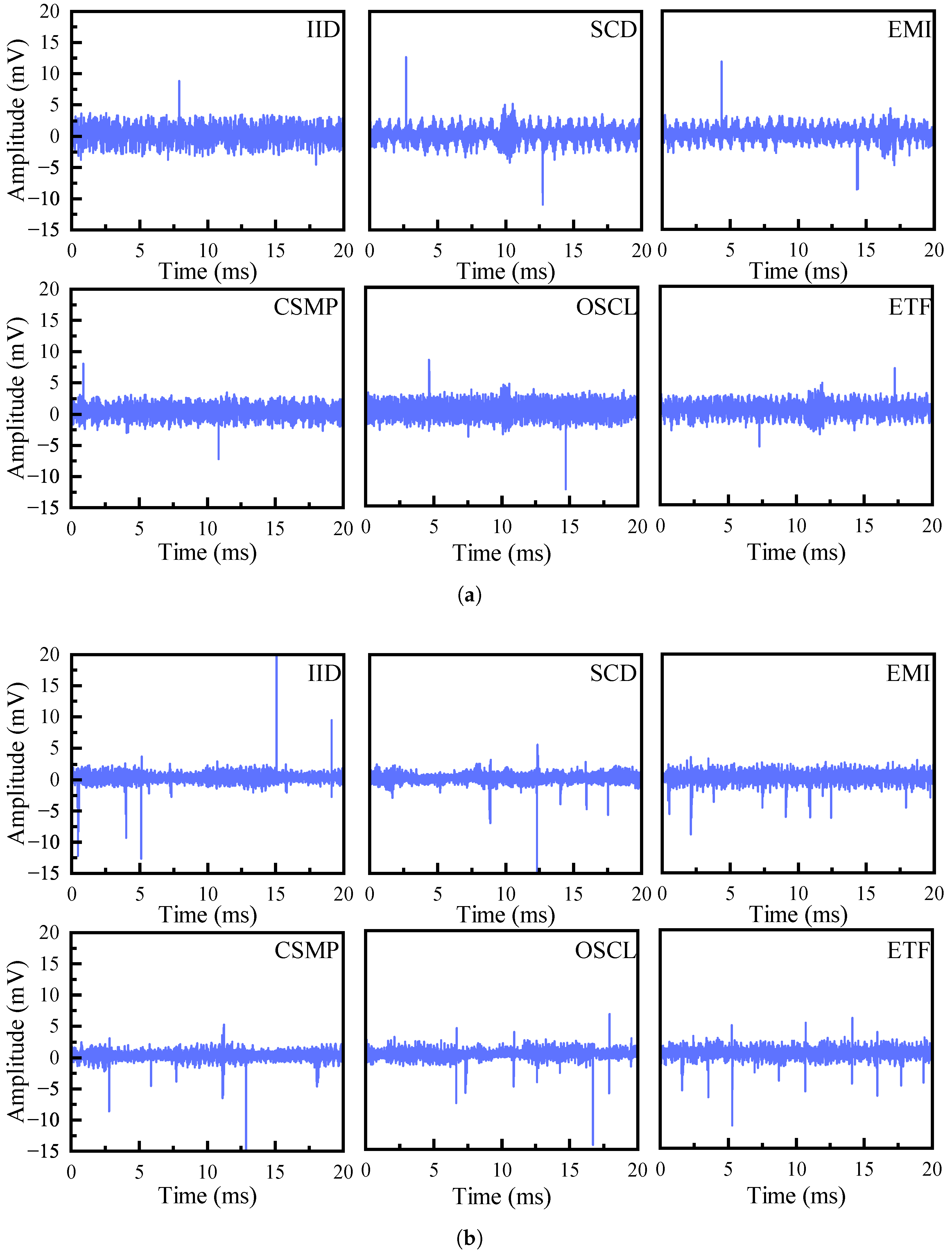
After mixing non-PD samples with two types of environmental noise samples, the constructed PDPR dataset is used to experimentally validate the effectiveness of the network model. The raw data, acquired under the experimental setup shown in Figure 4 using the oscilloscope, consist of 20 ms pulse-sequence waveforms (120,000 sampling points) representing single-pulse discharge amplitude sequences. These raw samples are presented in Figure 5a,b, with each group of samples randomly divided into training, validation, and test sets in a ratio of 6:2:2.
In the data processing phase, the raw signal is conveniently filtered using a Butterworth filter, and features are extracted as described in Section 2.3. During the training phase, the proposed DecPD model and the adaptive FL for the PD scenarios are used. The network model is configured with an initial learning rate of 0.01 and a batch size of 64. It is worth noting that, to ensure the robustness of the proposed method and avoid the influence of random initialization and stochastic training effects, all experiments reported in this work are conducted using ten-fold cross-validation. The results presented represent the average performance across the folds. This procedure guarantees that the evaluation reflects consistent model behavior rather than a single, potentially biased simulation.
The hardware environment is AMD Ryzen 7-4800H CPU @ 2.90 GHz 4.20 GHz, with a memory size of 16 GB, developed using the PyTorch 1.12.0 open-source framework under Python 3.9 of Windows 10 operating system.

3.3. Evaluation of Method

3.3.1. Comparison of Butterworth Filter Performance

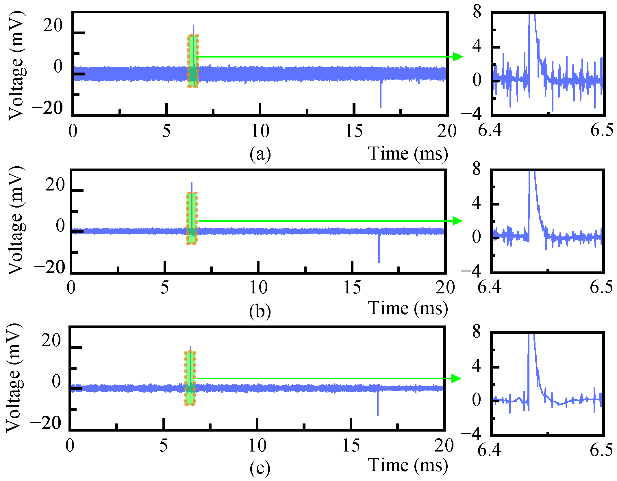
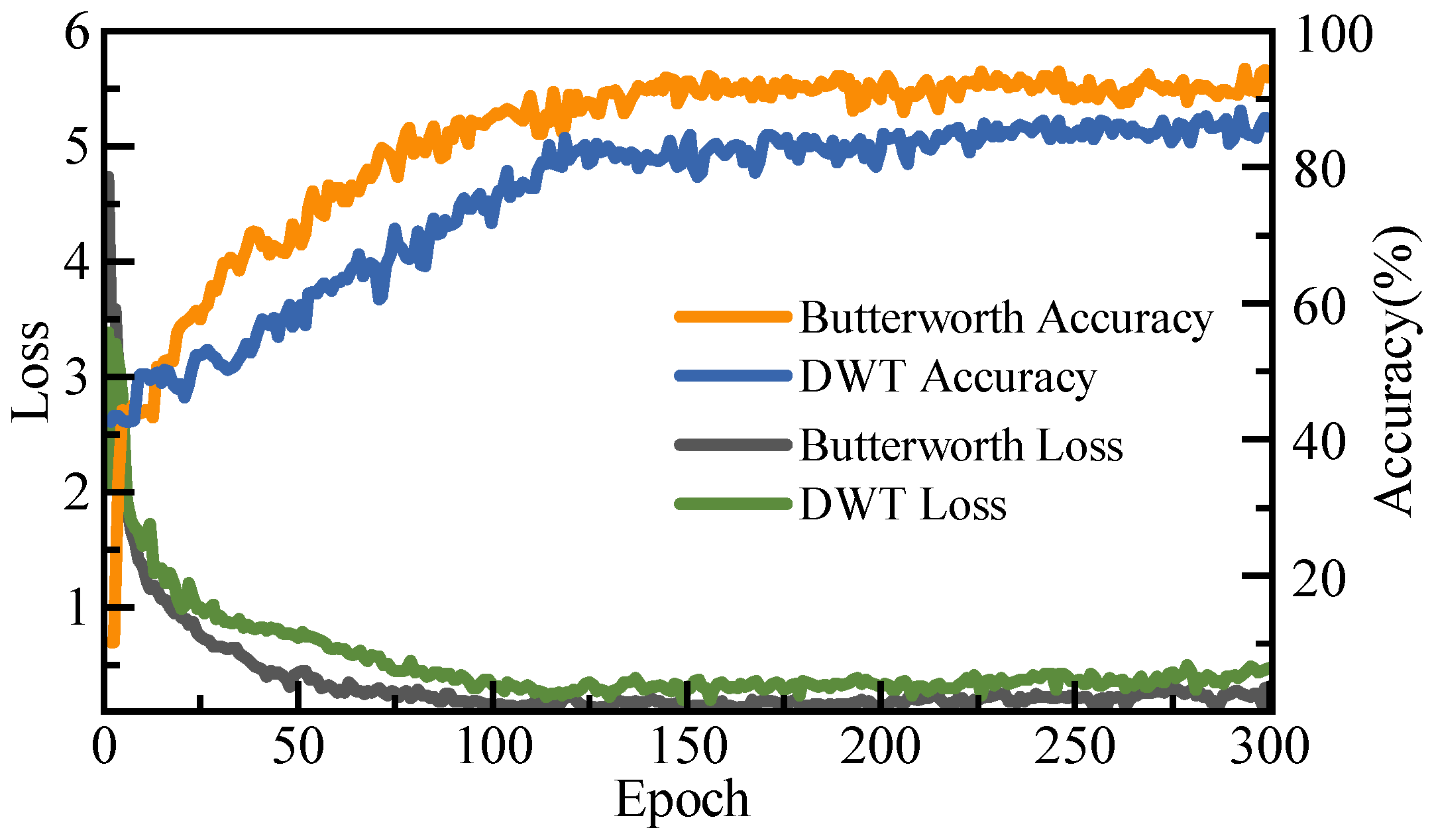
To validate that the Butterworth filter can achieve good performance with a simple design, the experimental parameters are set as follows: a threshold ratio of 0.3, a filter order of 4, and a cutoff frequency range of [15, 45], determined through (2)–(6), based on a sampling frequency of 50 Hz from the underlying power grid. Figure 6 shows a waveform comparison of the PD signal after filtering with the Butterworth filter and DWT. It is evident that the Butterworth filter, through the simple selection of the cutoff frequency range, reduces the environmental noise in the overall samples while preserving the waveform trend information in the PD samples.
The DWT method, when carefully designed as outlined in [22], can achieve results similar to those of DWT. However, since DWT decomposes the signal into sub-bands of different frequencies, an improper selection of the mother wavelet and decomposition level can easily lead to over-denoising, resulting in the loss of signal trends. For PDPR, the trend of PD pulses is crucial for the network model, loss of signal trend details will make recognition impossible. The experimental results are shown in Figure 7. Note that multiple sets of mother wavelets and decomposition levels were tested in the experiment, but none achieved the classification accuracy of the Butterworth filter.

3.3.2. Effectiveness of the DecPD Model

To assess the effectiveness of the DecPD model, the impacts of the dual-channel learning architecture, GRU, and DenseNet components on model performance were evaluated separately, the design of the four configuration groups is as follows: Group 1 employs the DecPD network model; Group 2 excludes the GRU component; Group 3 replaces the parallel structure with a serial structure; and Group 4 uses Softmax as the classifier.
Note that the standalone CNN and BiLSTM components, which are still used in existing advanced methods, will be compared with the overall approach of other works in the subsequent Section 3.4 through experimental analysis.
In this study, ablation studies were conducted on the above configurations to systematically evaluate the contribution of each module in the neural network model. The experimental results are shown in Table 2.
To investigate the impact of the GRU component, PDPR was performed by removing the GRU component from the DecPD model. Due to the lack of short-term temporal features and the inability of the attention mechanism to collaborate with the GRU, the overall accuracy decreased by 11.16% and the F1 score dropped by 17.41%. This undoubtedly underscores the importance of the GRU in complementing the feature information learned in parallel. In Group 3, although the network model with the serial structure showed faster training per epoch, it still exhibited an average gap of about 3% in accuracy and F1 score compared to the DecPD model. In Group 4, replacing DenseNet with only Softmax as the classifier not only increased the training time but also reduced accuracy by 7.36%, indicating that using dense blocks to enhance recognition accuracy is both reasonable and effective.

3.3.3. Effectiveness of the Adaptive FL

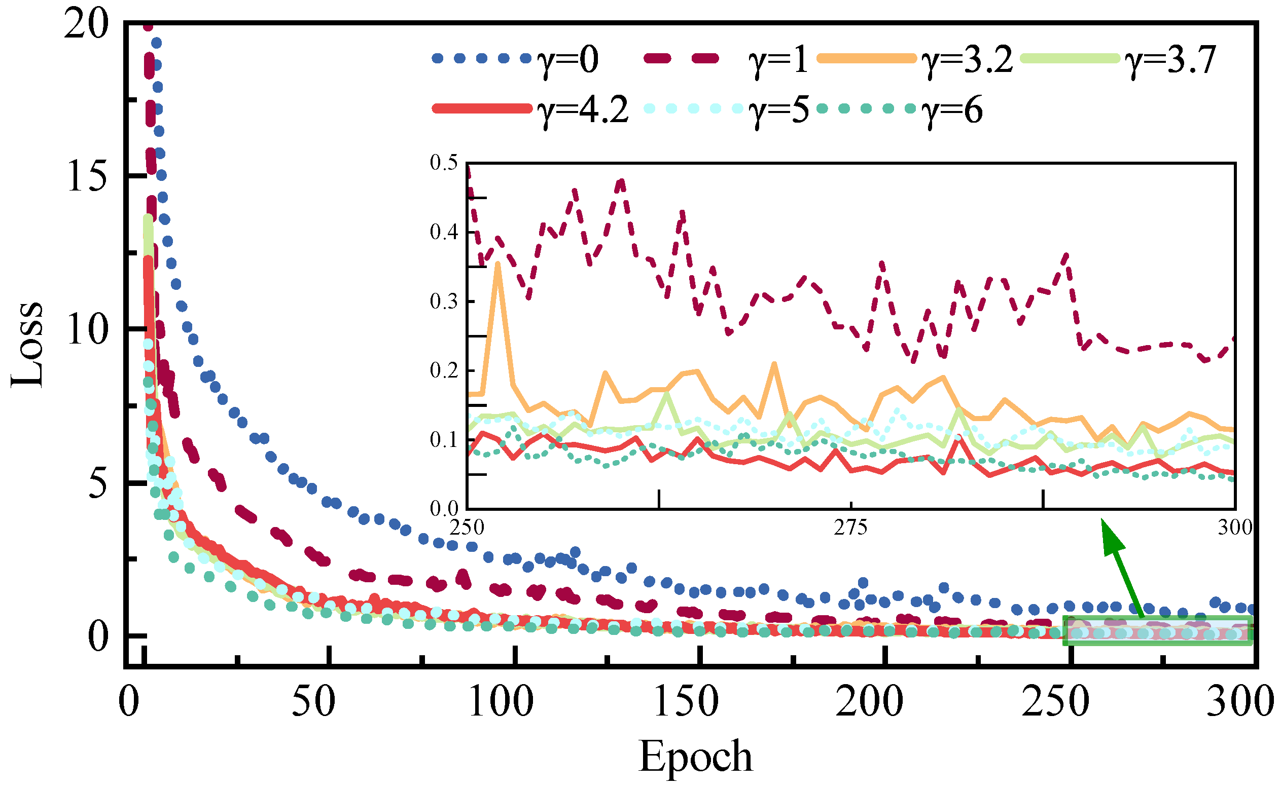
To refine the FL and reduce tuning time, a peak factor was applied to the adjustable focusing parameter. The average value of p a r in the PD dataset is 3.2, the balancing factor α c is set based on the inverse class frequency, with values of [1, 0.2, 0.2, 0.2, 0.2, 0.2, 0.2], and the value of γ ranges from 3.2 to 4.2. The overall value of γ was varied in stages and compared with the proposed improved focusing parameter form. The model iteration process is shown in Figure 8 and Table 3. As the overall value of γ increases, the loss function converges more quickly, which further affects simpler examples with low loss.
When γ = 0, the loss function corresponds to the original cross-entropy (CE), resulting in slower convergence and a higher final loss value. As γ is selected near 3 using the peak factor, the overall loss stabilizes around 0.1. However, if γ exceeds 5, the decrease in loss becomes more gradual, and excessive focus on complex examples results in a 3.6% drop in prediction accuracy compared to the baseline. Overall, by selecting the adjustable focusing parameter based on the peak factor, the model can adaptively choose hyper-parameters while maintaining prediction accuracy, effectively improving model performance by addressing class imbalance.

3.4. Comparison with Existing Approaches

In order to assess the performance of the proposed PDPR method, this section compares it with existing similar works, as summarized in Table 4. The work in [22] presents a typical method from a well-known PD dataset (vsb-power-line-fault-detection, 2018, Kaggle). Furthermore, the work in [43] developed a BiLSTM-based approach for PD detection, employing pulse arrival time differences for simultaneous defect type classification. Additionally, the work in [4] introduced a Physics-Informed Temporal Convolutional Network (PITCN), which explicitly incorporates physical knowledge of background noise and PD pulse characteristics into the learning framework. The work presented in [6] proposed a Multitask Learning Network (MLTN) architecture, taking severity assessment as the main task, diagnosis and localization as parallel auxiliary tasks.
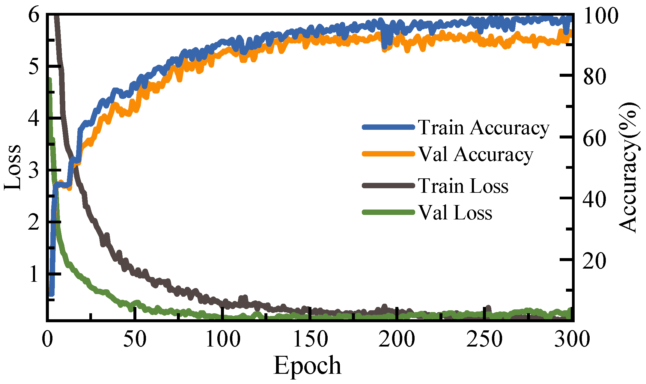
In addition to the overall accuracy, the evolution of loss and accuracy during the training and validation phases is visually presented in Figure 9.
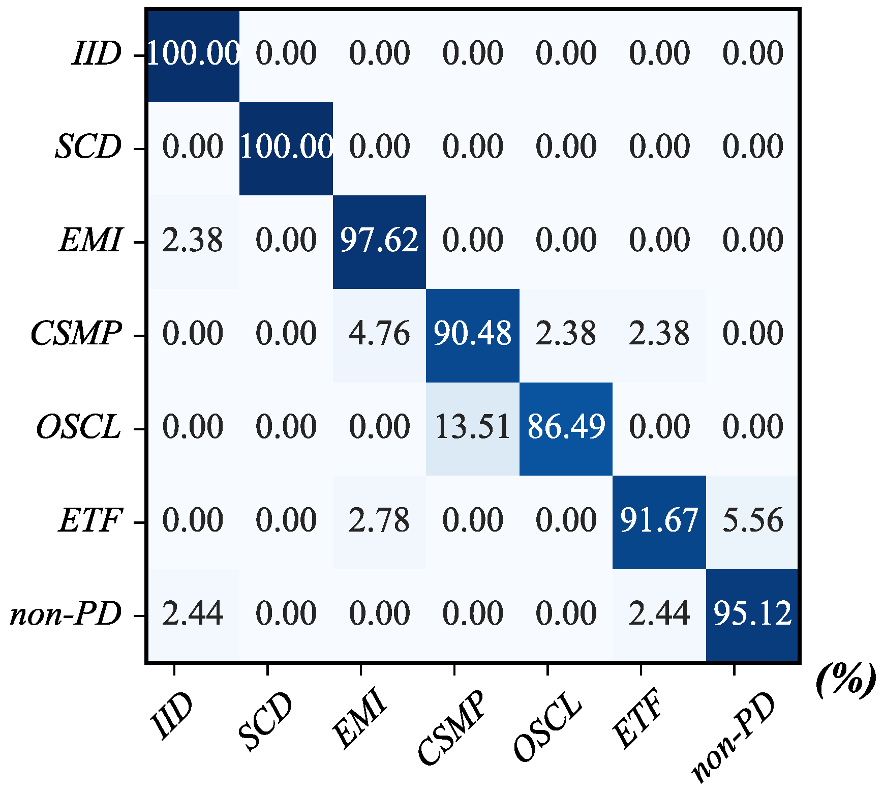
Furthermore, the confusion matrices of the PDPR under two types of environmental noise in the DecPD model, shown in Figure 10, reveal that the model has some difficulty distinguishing between EMI and CSMP defects. This is primarily because both types of partial discharge originate from metallic particles, which induce similar local physical effects. The main difference lies in the location of the particles within the cable insulation: EMI corresponds to embedded metallic particles causing conductive inclusions within the insulation, whereas CSMP arises from metallic particles on conductor surfaces under alternating electric fields. Since the underlying physical mechanism is similar but the spatial location differs subtly, the extracted features may not fully capture these distinctions, leading to occasional misclassification between these two classes.

4. Conclusions

In this study, a refined PDPR method based on the proposed DecPD model is developed to address the challenges of multi-type PD recognition under realistic noise conditions. The case studies highlight several key technical benefits of the framework. By combining a parallel CNN–BiLSTM architecture with the GRAttention mechanism, DecPD effectively captures both long-term temporal dependencies and short-transient PD characteristics, enabling accurate discrimination among highly similar defect types and substantially improving multi-class performance. The adaptive focal loss further enhances robustness against severe class imbalance by introducing a peak factor as an adaptive modulation term, allowing the model to focus on sparse hard samples without manual hyperparameter tuning and improving both stability and training efficiency. Moreover, validation on a real-world dataset acquired from the PD generation and measurement platform demonstrates that the proposed method maintains high accuracy under strong environmental noise, confirming its practical applicability.
Despite these advantages, the confusion matrix indicates that misclassification still occurs between EMI and CSMP, and the model shows limited capability in identifying metallic particle–induced PD. In addition, the current architecture introduces redundancy and increases computational cost. Future work will therefore focus on improving discrimination of metallic particle–related PD, reducing model complexity, and further enhancing noise robustness to support deployment in distributed and multi-regional online PDPR systems.

Author Contributions

Conceptualization, Y.W. and H.Y.; methodology, Y.W. and H.Y.; software, Y.W.; validation, S.L., Y.W. and H.Y.; formal analysis, Y.W.; investigation, H.Y.; resources, H.Y.; data curation, S.L.; writing—original draft preparation, Y.W.; writing—review and editing, Y.W.; visualization, Y.W.; supervision, Y.W. and F.G.; project administration, F.G.; funding acquisition, F.G.; Y.W. and H.Y. contributed equally to this work. All authors have read and agreed to the published version of the manuscript.

Funding

This research was funded by the National Natural Science Foundation of China, grant number 62373328.

Data Availability Statement

Data are contained within the article.

Acknowledgments

We sincerely thank Jie Sun from the Teizhou Power Supply Company of State Grid Zhejiang Electric Power Co. for providing valuable professional guidance on data collection and the operation of the experimental equipment.

Conflicts of Interest

The authors declare no conflicts of interest.

Abbreviations

The following abbreviations are used in this manuscript:
PDPRPartial Discharge Pattern Recognition
PDPartial Discharge
DecPDDeconstructed Partial Discharge
HVHigh Voltage
DLDeep Learning
CNNConvolutional Neural Network
LSTMLong Short-Term Memory
BiLSTMBidirectional Long Short-Term Memory
GRAttentionGated Recurrent Unit Attention
DWTDiscrete Wavelet Transform
FLFocal Loss
FFTFast Fourier Transform
PSDPower Spectral Density
DenseNetDense Network
GRUGated Recurrent Unit
PEIPower Electronic Interference
XLPECross-Linked Polyethylene
HFCTHigh-Frequency Current Transformer
CECross Entropy
PITCNPhysics-Informed Temporal Convolutional Network
MLTNMultitask Learning Network

References

  1. Khan, Q.; Refaat, S.S.; Abu-Rub, H.; Toliyat, H.A.; Olesz, M.; Darwish, A. Characterization of Defects Inside the Cable Dielectric with Partial Discharge Modeling. IEEE Trans. Instrum. Meas. 2021, 70, 3502911. [Google Scholar] [CrossRef]
  2. Ren, J.; Ma, Y.; Qu, Q.; Wang, Z.; Wang, Y.; Wang, L.; Han, X.; Yang, X. Study on Partial Discharge Characteristics of Mixed Metal Particles Under Combined Power Frequency and Switching Impulse Voltage. Energies 2025, 18, 5650. [Google Scholar] [CrossRef]
  3. Negri, V.; Mingotti, A.; Tinarelli, R.; Peretto, L.; Ray, L.S.S.; Zhou, B.; Lukowicz, P. A Novel Health Index for MV Cable Joint Aging Prediction Based on Dynamic Graph Attention Model. IEEE Trans. Instrum. Meas. 2025, 74, 2516608. [Google Scholar] [CrossRef]
  4. Lu, G.; Tsang, C.W.; Yim, H.N.; Lei, C.; Bu, S.; Yung, W.K.C.; Pecht, M. Interpretable Fault Diagnosis for Overhead Lines with Covered Conductors: A Physics-Informed Deep Learning Approach. Prot. Control Mod. Power Syst. 2025, 10, 25–39. [Google Scholar] [CrossRef]
  5. Hu, H.; Li, X.; Wang, Z.; Jia, Z. Moisture Degradation Characteristics and Multi-Performance-Based Status Assessment Method of Distribution Cables. IEEE Trans. Power Del. 2024, 39, 3017–3027. [Google Scholar] [CrossRef]
  6. Wang, Y.; Yan, J.; Zhang, W.; Yang, Z.; Wang, J.; Geng, Y.; Srinivasan, D. Mutitask Learning Network for Partial Discharge Condition Assessment in Gas-Insulated Switchgear. IEEE Trans. Ind. Inform. 2024, 20, 11998–12009. [Google Scholar] [CrossRef]
  7. Zhu, T.; Lin, Y.; Tian, H.; Yan, Y. A Cable Partial Discharge Localization Method Based on Complete Ensemble Empirical Mode Decomposition with Adaptive Noise–Multiscale Permutation Entropy–Improved Wavelet Thresholding Denoising and Cross-Correlation Coefficient Filtering. Energies 2025, 18, 5511. [Google Scholar] [CrossRef]
  8. Jing, X.; Wu, Z.; Zhang, L.; Li, Z.; Mu, D. Electrical Fault Diagnosis From Text Data: A Supervised Sentence Embedding Combined With Imbalanced Classification. IEEE Trans. Ind. Electron. 2024, 71, 3064–3073. [Google Scholar] [CrossRef]
  9. Hu, Y.; Chang, H.; Wang, H.; Wu, Q.; Zhang, C.; Ren, M.; Dong, M. Lightweight Diagnosis of Short-Gap Arcs in Oil-Paper Insulation Based on Depthwise Separable CNN. IEEE Trans. Instrum. Meas. 2025, 74, 3510111. [Google Scholar] [CrossRef]
  10. Ganguly, B.; Chaudhuri, S.; Biswas, S.; Dey, D.; Munshi, S.; Chatterjee, B.; Dalai, S.; Chakravorti, S. Wavelet Kernel-Based Convolutional Neural Network for Localization of Partial Discharge Sources Within a Power Apparatus. IEEE Trans. Ind. Inform. 2021, 17, 1831–1841. [Google Scholar] [CrossRef]
  11. Wang, Y.; Yan, J.; Yang, Z.; Xu, Z.; Qi, Z.; Wang, J.; Geng, Y. Simultaneous Partial Discharge Diagnosis and Localization in Gas-Insulated Switchgear via a Dual-Task Learning Network. IEEE Trans. Power Del. 2023, 38, 4358–4370. [Google Scholar] [CrossRef]
  12. Zheng, S.; Liu, J.; Zeng, J. MDTCNet: A Novel Multiscale Denoising Transformer Convolutional Network for Fault Diagnosis of Partial Discharge. IEEE Trans. Dielectr. Electr. Insul. 2025, 32, 2938–2947. [Google Scholar] [CrossRef]
  13. Kumar, C.; Ganguly, B.; Dey, D.; Chatterjee, S. Multi-Scale CNN-LSTM Network for Denoising Acoustic Partial Discharge Signal in an Electrical Apparatus. Arab. J. Sci. Eng. 2025, 1–19. [Google Scholar] [CrossRef]
  14. Fu, Z.; Wang, Y.; Zhou, L.; Li, K.; Rao, H. Partial Discharge Recognition of Transformers Based on Data Augmentation and CNN-BiLSTM-Attention Mechanism. Electronics 2025, 14, 193. [Google Scholar] [CrossRef]
  15. Priananda, C.W.; Illias, H.A.; Raymond, W.J.K.; Negara, I.M.Y. Hybrid Deep Learning Models for Enhanced Classification of Phase-Resolved Partial Discharge Patterns from High-Voltage Rotating Machine Insulation. IEEE Trans. Dielectr. Electr. Insul. 2025, 32, 3059–3067. [Google Scholar] [CrossRef]
  16. Liu, H.; Zhang, Z.; Song, R.; Shu, Z.; Wang, J.; Tian, H.; Song, Y.; Chen, W. Pattern Recognition Method for Detecting Partial Discharge in Oil-Paper Insulation Equipment Using Optical F-P Sensor Array Based on KAN-CNN Algorithm. J. Light. Technol. 2025, 43, 6004–6012. [Google Scholar] [CrossRef]
  17. Liu, J.; Wang, S.; Zhang, H.; Zhang, M.; Sun, W. Diagnosis and Location of Cable Defects Based on Digital Reconstruction of Impedance Spectrum Under Pseudotrapezoidal PFM Excitation. IEEE Trans. Ind. Electron. 2023, 70, 11754–11763. [Google Scholar] [CrossRef]
  18. Yu, S.; Wang, J.; Gou, B.; Xie, C. A Novel Bilateral Branching Network With Cost-Sensitive Res2Net for Diagnosis GIS Insulation Defects on Imbalanced Data. IEEE Trans. Instrum. Meas. 2024, 73, 3537811. [Google Scholar] [CrossRef]
  19. Wang, Y.; Yan, J.; Yang, Z.; Jing, Q.; Wang, J.; Geng, Y. GAN and CNN for imbalanced partial discharge pattern recognition in GIS. High Voltage 2022, 7, 452–460. [Google Scholar] [CrossRef]
  20. Ji, J.; Shu, Z.; Li, H.; Lai, K.X.; Lu, M.; Jiang, G.; Wang, W.; Zheng, Y.; Jiang, X. Edge-Computing-Based Knowledge Distillation and Multitask Learning for Partial Discharge Recognition. IEEE Trans. Instrum. Meas. 2024, 73, 3537811. [Google Scholar] [CrossRef]
  21. Lin, T.Y.; Goyal, P.; Girshick, R.; He, K.; Dollár, P. Focal loss for dense object detection. In Proceedings of the IEEE International Conference on Computer Vision, Venice, Italy, 22–29 October 2017; pp. 2980–2988. [Google Scholar]
  22. Misák, S.; Fulnecek, J.; Vantuch, T.; Buriánek, T.; Jezowicz, T. A complex classification approach of partial discharges from covered conductors in real environment. IEEE Trans. Dielectr. Electr. Insul. 2017, 24, 1097–1104. [Google Scholar] [CrossRef]
  23. Liu, M.; Yang, B.; Meng, L.; Zhang, Y.; Gao, S.; Zan, P.; Xia, X. STA-Net: Spatial–temporal alignment network for hybrid EEG-fNIRS decoding. Inf. Fusion 2025, 119, 103023. [Google Scholar] [CrossRef]
  24. Klein, L.; Seidl, D.; Fulneček, J.; Prokop, L.; Mišák, S.; Dvorskỳ, J. Antenna contactless partial discharges detection in covered conductors using ensemble stacking neural networks. Expert Syst. Appl. 2023, 213, 118910. [Google Scholar] [CrossRef]
  25. Chen, K.; Vantuch, T.; Zhang, Y.; Hu, J.; He, J. Fault detection for covered conductors with high-frequency voltage signals: From local patterns to global features. IEEE Trans. Smart Grid 2020, 12, 1602–1614. [Google Scholar] [CrossRef]
  26. Karimi, M.; Majidi, M.; MirSaeedi, H.; Arefi, M.M.; Oskuoee, M. A Novel Application of Deep Belief Networks in Learning Partial Discharge Patterns for Classifying Corona, Surface, and Internal Discharges. IEEE Trans. Ind. Electron. 2020, 67, 3277–3287. [Google Scholar] [CrossRef]
  27. Li, Q.; Xu, Y.; Cho, S.; Suo, C.; Yip, T.T.L. Health Assessment of Underground Power Cables: A Data-Driven Approach Based on One-Sample Maximum Mean Discrepancy. IEEE Trans. Power Deliv. 2025, 40, 2443–2446. [Google Scholar] [CrossRef]
  28. Fei, Z.; Li, Y.; Yang, S. Partial Discharge Pattern Recognition Based on an Ensembled Simple Convolutional Neural Network and a Quadratic Support Vector Machine. Energies 2024, 17, 2443. [Google Scholar] [CrossRef]
  29. Han, G.; Zhao, X.; Sun, X.; Zhao, S.; Duan, H.; Liu, X.; Li, Q. Analysis on the Growth Mechanism of Electrical Treeing in Transmission Cables. IEEE Trans. Dielectr. Electr. Insul. 2025, 74, 3506511. [Google Scholar] [CrossRef]
  30. Sharma, A.; Devarajan, H.; Govindarajan, S.; Shanker, T.B.; Ardila Rey, J.A.; Nandi, S. High-Confidence Classification of Partial Discharge Acoustic Signals Using Bayesian Networks for Uncertainty Quantification. IEEE Trans. Instrum. Meas. 2025, 74, 3506511. [Google Scholar] [CrossRef]
  31. Zhang, Z.; Chen, W.; Wu, K.; Liu, H.; Chen, X.; Jiang, T.; Ma, Z.; Feng, W. Novel Approach for Partial Discharge Localization Based on Fiber-Optic FP Sensing Array and Modified TDOA in a 110 kV Transformer. IEEE Trans. Instrum. Meas. 2024, 73, 9517711. [Google Scholar]
  32. Wu, Q.; Dong, C.; Guo, F.; Wang, L.; Wu, X.; Wen, C. Privacy-Preserving Federated Learning for Power Transformer Fault Diagnosis With Unbalanced Data. IEEE Trans. Ind. Inform. 2024, 20, 5383–5394. [Google Scholar] [CrossRef]
  33. Guo, F.; Li, S.; Yang, H.; Dong, C.; Chen, Y.; Li, G. An Efficient Sequential Decentralized Federated Progressive Channel Pruning Strategy for Smart Grid Electricity Theft Detection. IEEE Trans. Ind. Inform. 2025, 21, 2393–2402. [Google Scholar] [CrossRef]
  34. Ye, J.; Lv, J.; Xu, G.; Liu, T. Leaky Cable Perimeter Intrusion Detection Based on Deep Reinforcement Learning. IEEE Internet Things J. 2024, 11, 22616–22627. [Google Scholar] [CrossRef]
  35. Chen, H.; Jiang, D.; Sahli, H. Transformer Encoder With Multi-Modal Multi-Head Attention for Continuous Affect Recognition. IEEE Trans. Multimed. 2021, 23, 4171–4183. [Google Scholar] [CrossRef]
  36. Li, G.; Zhang, M.; Li, J.; Lv, F.; Tong, G. Efficient densely connected convolutional neural networks. Pattern Recognit. 2021, 109, 107610. [Google Scholar] [CrossRef]
  37. Huang, Z.; Sang, Y.; Sun, Y.; Lv, J. A neural network learning algorithm for highly imbalanced data classification. Inf. Sci. 2022, 612, 496–513. [Google Scholar] [CrossRef]
  38. Liu, K.; Jiao, S.; Nie, G.; Ma, H.; Gao, B.; Sun, C.; Xin, D.; Saha, T.K.; Wu, G. On image transformation for partial discharge source identification in vehicle cable terminals of high-speed trains. High Volt. 2024, 9, 1090–1100. [Google Scholar] [CrossRef]
  39. Li, A.; Wei, G.; Zhang, J.; Zhang, C. Partial Discharge Detection via Self-Supervised Graph Contrastive Clustering. IEEE Trans. Ind. Inform. 2025, 21, 4016–4026. [Google Scholar] [CrossRef]
  40. IEC 60270; High-Voltage Test Techniques—Partial Discharge Measurements. IEC: Geneva, Switzerland, 2000.
  41. Zhu, M.; Shi, F.; Yan, Y.; Li, H. A Method for Constructing Short-Time AC Voltage Generator to Evaluate Cable Conditions. IEEE Trans. Ind. Electron. 2025, 72, 2078–2088. [Google Scholar] [CrossRef]
  42. Hu, X.; Siew, W.H.; Judd, M.D.; Reid, A.J.; Sheng, B. Modeling of high-frequency current transformer based partial discharge detection in high-voltage cables. IEEE Trans. Power Del. 2019, 34, 1549–1556. [Google Scholar] [CrossRef]
  43. Bhukya, A.; Koley, C. Bi-Long Short-Term Memory Networks for Radio Frequency Based Arrival Time Detection of Partial Discharge Signals. IEEE Trans. Power Del. 2022, 37, 2024–2031. [Google Scholar] [CrossRef]
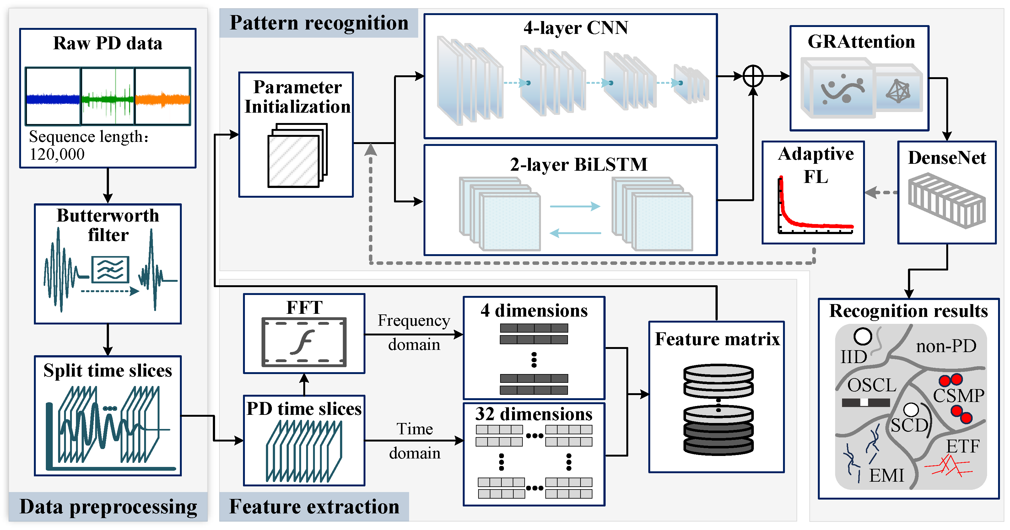
Figure 1. Block diagram of PDPR based on the DecPD network model.
Energies 18 06245 g001
Figure 2. The detailed structure and dimensions of the DecPD network model.
Energies 18 06245 g002
Figure 3. The cable structure and artificial defect. (a) Cable. (b) Cross section. (c) Longitudinal section.
Energies 18 06245 g003
Figure 4. HV laboratory equipment for PD measurement. (a) PD data generation platform. (b) Equipment and testing laboratory.
Energies 18 06245 g004
Figure 5. The typical raw data graph of six defects under environmental noise. (a) Under white noise. (b) Under PEI. Note: The horizontal axis represents 20 ms of acquisition time (120,000 sampling points), and the vertical axis indicates the discharge-amplitude values. Since the full 120,000 points are too dense for direct visualization, the plot is generated by dividing the sequence into 10,000 groups and using the mean of every 12 data points.
Energies 18 06245 g005
Figure 6. Comparison chart of PD sample filtering effect. (a) Origin signal. (b) DWT method. (c) Butterworth method.
Energies 18 06245 g006
Figure 7. The loss and accuracy curves of the DecPD model under different filtering methods on the validation dataset.
Energies 18 06245 g007
Figure 8. Loss curves of the DecPD model under different γ values.
Energies 18 06245 g008
Figure 9. Loss and accuracy curves of the DecPD model during the training and validation phases.
Energies 18 06245 g009
Figure 10. Confusion matrices of the test dataset obtained using the proposed PDPR method under environmental noise.
Energies 18 06245 g010
Table 1. PD datasets distribution for each type of defect.
Primary CategoriesRefined TypesNumber of Samples
Internal dischargeIID458
ETF444
EMI440
Surface dischargeCSMP449
OSCL431
Corona dischargeSCD446
Non-PD/3000
Table 2. Ablation experiment evaluation results of the DecPD model.
MetricsGroup 1Group 2Group 3Group 4
Accuracy (%)96.6585.4993.7589.29
Recall (%)94.4877.5190.4083.91
Precision (%)95.2878.7791.1383.32
F1 Score (%)94.8277.4190.6583.56
Time (s)4.504.102.704.60
Table 3. Accuracy and training time of the DecPD model under different γ values.
Loss Function α Value γ ValueAccuracy (%)Time (s)
Cross Entropy/095.749.8
Focal Loss/195.548.6
/592.554.2
/688.614.1
Adaptive FL3.2096.054.9
0.53.796.654.5
14.293.384.4
Table 4. Comparison with some state-of-the-art methods on the PD recognition dataset.
MethodAccuracy (%)Time (s)
DecPD96.654.5
DWT+CNN [22]91.800.65
Pulse-Position+BiLSTM [43]82.200.82
PITCN [4]87.521.21
MTLN [6]93.252.30
Disclaimer/Publisher’s Note: The statements, opinions and data contained in all publications are solely those of the individual author(s) and contributor(s) and not of MDPI and/or the editor(s). MDPI and/or the editor(s) disclaim responsibility for any injury to people or property resulting from any ideas, methods, instructions or products referred to in the content.