Abstract
The high proportion of wind power access makes the system frequency regulation face serious challenges, and the time delay of wind turbine FM response exacerbates the frequency security problem. For this reason, this paper proposes a joint dispatch model for power grid and wind farms considering frequency modulation delay. First, the wind turbine response characteristics and frequency safety constraints are derived by equivalently modeling the wind turbine FM delay. Second, power grid-wind farm joint dispatch model is constructed on this basis, where the system level optimizes the operation cost under the premise of satisfying the frequency safety constraints, and the wind farm level tracks the wind power output target issued by the system to meet the FM demand. Finally, by the case study, Scenario 1 reduces average frequency nadir deviation from 0.205 Hz to 0.098 Hz and RoCoF from 0.216 Hz/s to 0.168 Hz/s in the IEEE-39 system. The stability of the system is enhanced, which verifies the effectiveness of the proposed method.
1. Introduction
The global transition towards new power systems centered on renewable energy is driving a shift in wind power’s role, from passive grid integration to active grid support [1,2,3,4]. However, the inherent intermittency and volatility of wind power introduce unprecedented challenges to power system security and stability [5,6,7,8]. This is particularly critical in systems with high wind power penetration, where frequency regulation capabilities are severely strained [9,10,11]. In response, several countries have instituted grid codes mandating frequency response capabilities from wind power installations [12]. A significant challenge persists: wind turbines exhibit pronounced time delays in their frequency modulation (FM) response. Field tests from operational renewable power plants [13,14,15,16,17] reveal that these FM delays vary substantially across different wind farms and turbine models. Originating from measurement, signal processing, and control execution stages, these delays directly impair the effectiveness of frequency regulation and the system’s dynamic frequency response. Specifically, excessive delays diminish the effective system inertia, aggravate the Rate of Change of Frequency (RoCoF), and amplify frequency deviations, thereby jeopardizing overall system stability.
Existing research on enhancing frequency stability in wind-integrated power systems can be broadly classified into three categories: control strategy improvements, system dispatch optimization, and emerging coordination frameworks. Despite these efforts, significant gaps remain, particularly in comprehensively addressing FM delays and establishing effective joint dispatch coordination.
Studies focusing on control strategy improvements aim to enhance the inherent frequency response performance of wind turbine generators. Various advanced control techniques have been proposed, including coordinated adaptive sliding mode control using radial basis function neural networks [18], auxiliary frequency control based on functional optimization models [19], and distributed frequency regulation methods [20,21]. While these approaches improve control performance to a certain degree, they largely rely on the idealistic assumption of an instantaneous wind turbine response. Consequently, they often fail to adequately account for the limitations that actual FM delays impose on achievable control performance. Although reference [22] employed Long Short-Term Memory neural networks to compensate for time delays, its scope is still limited to control optimization at the individual wind farm level, without integration into the broader context of grid-wide dispatch.
Research on system dispatch optimization primarily focuses on incorporating frequency security constraints into power system scheduling models. For instance, references [23,24] integrated constraints like RoCoF and frequency nadir into stochastic generation scheduling to ensure frequency security. Reference [25] developed a source-load-storage dynamic frequency response model for generation scheduling, while reference [26] addressed peak shaving demands while preserving frequency security. These contributions have significantly advanced the use of frequency security constraints in dispatch models. However, the constraints formulated in these studies typically depend on the response characteristics of conventional synchronous generators or idealized renewable units. A critical shortcoming is their failure to incorporate the impact of wind turbine FM delays into the dispatch model. This oversight can cause system operators to overestimate the available frequency regulation capacity from wind power, leading to a mismatch between the optimized generation schedule and the actual delayed response from wind farms. As a result, the practical effectiveness of the dispatch plan for frequency control is undermined.
Recognizing the limitations of isolated approaches, recent research has started to explore coordinated control and fundamental shifts in system architecture. For example, reference [27] designed an extended state observer with delay compensation for distributed optimal control, aiming to address physical constraints and time delays concurrently. A more transformative development is the advent of grid-forming (GFM) inverter control for wind turbines [28,29]. In contrast to conventional grid-following strategies, GFM control allows wind turbines to autonomously establish grid voltage and frequency, thereby inherently providing instantaneous inertial support and potentially alleviating the negative impacts of response delays. The validation of such advanced control strategies increasingly utilizes Hardware-in-the-Loop (HIL) testing [30,31], which offers a high-fidelity environment for evaluating controller performance under realistic delay conditions.
Despite these advancements, a clear and critical research gap remains: the translation of wind turbine FM delay characteristics from the local control level to the system-wide dispatch level has not been fully addressed. Specifically, studies such as [13] focus on modeling delays but do not apply them to dispatch problems. Conversely, works like [24,26,32] integrate frequency constraints into dispatch models but overlook the impact of wind power delays. Thus, effectively bridging this gap is necessary. The core contribution of this paper is to address this disconnect by proposing a joint grid-wind farm dispatch model. This model explicitly incorporates wind FM delays into the system-wide frequency security constraints, thereby ensuring consistency between dispatch commands and the actual dynamic response capabilities of wind farms.
In summary, a significant disconnect persists between the domains of “control” and “dispatch”. Research on control strategies often neglects to translate its considerations of time delays into applicable dispatch models. Simultaneously, studies on dispatch optimization frequently overlook time delays as a critical physical constraint. Therefore, developing a joint grid-wind farm dispatch model that explicitly accounts for wind turbine FM delays is essential. Such a model is crucial for aligning dispatch decisions with realistic system responses and for fundamentally enhancing the frequency security of power systems with high wind power penetration.
To address the identified gap, this paper proposes a joint dispatch model for power grids and wind farms that incorporates wind turbine frequency regulation delays. The methodology is as follows. First, a delay element is introduced into the traditional primary frequency response model of a wind turbine. This delay element is then approximated using a first-order Padé expansion, facilitating the derivation of a wind turbine frequency response model that explicitly accounts for the FM delay. Based on this enhanced model, system-wide frequency security constraints considering the wind turbine delay are formulated, and any nonlinearities in these constraints are linearized for tractability. Subsequently, a practical joint dispatch architecture for the grid and wind farms is established. Second, distinct optimization models are formulated for the grid-level and the wind-farm-level dispatch. The grid-level dispatch model minimizes total system operating cost while satisfying the proposed frequency security constraints that internalize the impact of wind FM delays. The wind-farm-level dispatch model aims to track the power output targets set by the grid-level dispatch by managing internal resources. Finally, case studies performed on a modified IEEE-39 bus system validate the proposed approach.
2. Modeling Dynamic Frequency Security Constraints Considering Wind Turbine Frequency Regulation Delays
In practical operation, the processes of inertia emulation and frequency regulation control in wind turbines involve inherent delays due to measurement, signal processing, and control execution [33]. These response delays degrade the effectiveness of frequency deviation suppression, prolong the system frequency recovery period, and may even induce secondary oscillations or frequency dips. Therefore, it is crucial to accurately represent these response delay characteristics in frequency response models.
2.1. Analysis of Wind Turbine Power Output Characteristics Considering Frequency Regulation Delay
The conventional primary frequency response model for wind turbines typically assumes a linear increase in output power and incorporates a frequency deadband, as expressed in Equation (1).
where tDB is the dead time, Td is the duration of the primary frequency response, RW is the maximum power output during the primary frequency response of the wind turbine, ΔPW(t) is the power output of the wind turbine during the primary frequency response at time t.
To accurately capture the response delay of wind turbines, a delay term e–τs is incorporated into the model described by Equation (1). To facilitate the integration of this delayed response into the dispatch optimization model, the irrational delay term is approximated using a first-order Padé expansion. This approximation remains valid under small-signal conditions and within the linear operating region of the wind turbine’s control system, which covers typical frequency regulation events. The adequacy of this approximation has been confirmed in prior work [13]. Consequently, the Padé approximation is adopted to represent the delay element equivalently, as given in Equation (2).
where G(s) is the frequency domain form of the frequency response characteristic of a wind turbine generator set considering frequency regulation delay, F(s) is the frequency domain form of the frequency response characteristic of a wind turbine generator set without considering frequency regulation delay, τ is the frequency regulation delay.
Applying the Laplace transform to the time-domain function in Equation (1) gives:
Substituting Equation (3) into Equation (2) results in:
The inverse Laplace transform of Equation (4) then yields the time-domain expression:
Thus, the complete frequency response model for a wind turbine, considering the frequency regulation delay, is formulated as:
The frequency regulation response characteristics of wind turbines considering frequency regulation delay are shown in Figure 1:
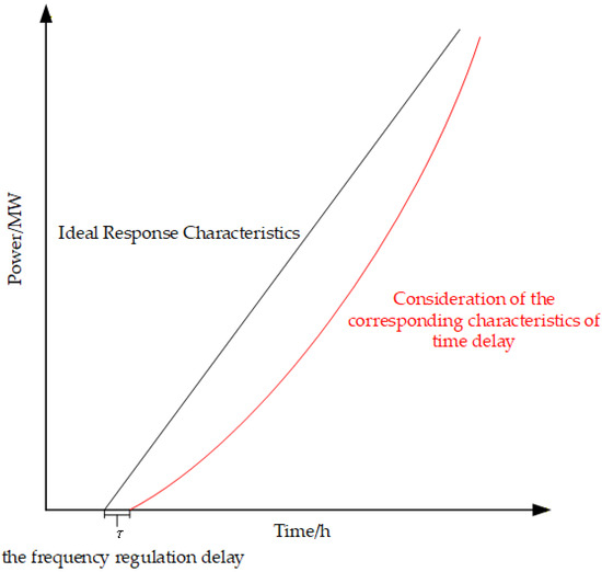
Figure 1.
Comparison Chart of Frequency Regulation Response Characteristics for Wind Turbine Generators.
2.2. Formulation of Frequency Security Constraints Considering Wind Turbine Delay
To derive tractable frequency security constraints for the dispatch model, a quasi-steady-state approach is adopted for each scheduling interval. This approach assumes that the system inertia M(t) and the potential power disturbance magnitude remain constant within a given time period t, based on the pre-dispatch schedule. This simplification allows the system frequency dynamics following a disturbance to be described by an ordinary differential equation, which can be solved analytically for each time step [22]:
where M(t) is the total inertia of the system at time t, f0 is the rated frequency of the system, Δf(t) is the frequency deviation of the system at time t, D is the load damping coefficient, PL(t) is the total load of the system at time t, ΔPG(t) is the response power of the conventional frequency-regulating units at time t, is the load disturbance at time t.
By incorporating the wind turbine delay model from Equation (6) into the system dynamics, the frequency evolution equation becomes:
Solving Equation (8) yields the key system frequency security metrics—namely, the Rate of Change of Frequency (RoCoF), the frequency nadir (maximum frequency deviation), and the quasi-steady-state frequency deviation—while accounting for the wind turbine delay [32].
The frequency security constraints derived in this section—specifically for RoCoF and frequency nadir—are based on a simplified yet widely adopted analytical framework [26]. This framework models a single, large power disturbance, representing the most severe credible contingency for frequency stability assessment. The linearized power response models for both conventional generators and wind units yield a conservative estimate of the system’s frequency response. Although this approach does not capture the full spectrum of dynamic interactions or continuous small disturbances, it provides a tractable and effective set of constraints for pre-dispatch planning, ensuring a robust defense against critical frequency events.
- (1)
- RoCoF Constraint
Immediately following a power disturbance, and before the frequency deviation exceeds the deadband, the active power response from all frequency-regulating units is zero. Consequently, the initial RoCoF is determined solely by the system inertia and the magnitude of the power imbalance, as given by:
where H(t) is the total inertia of the system at time t.
The total system inertia is calculated as the sum of the inertia contributions from all online synchronous generators and wind farms [26]:
where ug,t is the start/stop status of thermal power unit g at time t, hg and hw is the inertia time constants of thermal power units and wind power units, respectively, G and W is the total number of thermal power units and wind farms, respectively, Sg and Sw is the installed capacity of thermal power units and wind farms, respectively.
It is worth noting that the quasi-static assumption decouples the temporal dependencies of M(t) across different dispatch intervals, significantly simplifying the model for optimization. While this approach does not capture the inter-temporal coupling of inertia during the transient itself, it provides a conservative and computationally efficient estimate for ensuring frequency security in the pre-dispatch phase.
To maintain system stability, the maximum permissible RoCoF must not be exceeded. This leads to the following RoCoF security constraint:
where RoCoFmax is the maximum RoCoF value for the system.
- (2)
- Frequency Level at Nadir
When the frequency change rate is zero, the system frequency deviation reaches its frequency level at the nadir. Substituting the specific functional forms of wind turbines and conventional thermal power frequency regulation units into Equation (8), the functional form for conventional thermal power frequency regulation units is identical to Equation (1) and is not repeated here, yielding:
where RG is the maximum power output during primary frequency regulation response for thermal power units.
By integrating, we obtain the expression for the absolute value of the system frequency deviation:
When t ≥ tDB, let , yields:
where t* is the time at which the system reaches the frequency level at nadir.
Therefore, the frequency level at nadir is:
The frequency level at nadir of the system must not exceed the limit value. The frequency level at nadir constraint is:
where Δfmax is the frequency level at nadir limit.
Since this constraint is nonlinear, transformation processing is required. Since the value of t* is determined by H(t), Equation (15) reveals a function of H(t). Monotonicity analysis shows that as H(t) increases, the maximum frequency difference in the system decreases, making the function monotonically decreasing. Therefore, a unique solution H(t*s) exists such that =Δfmax holds. Equation (16) can be transformed into:
where yg,t are auxiliary variables, M is a sufficiently large number.
- (3)
- Frequency Level at Quasi-Steady-State
When the system reaches a frequency steady state, the frequency change rate is zero. At this point, the system frequency deviation is primarily determined by the response power of the frequency-modulating units. The frequency level at quasi-steady-state is approximated by:
where tss is the time at which the system reaches the frequency level at quasi-steady-state.
The frequency level at quasi-steady-state of the system must not exceed the limit value. The frequency level at quasi-steady-state constraint is:
where Δfssmax is maximum frequency level at quasi-steady-state.
3. Joint Dispatch Architecture for Power Grid and Wind Farms
The integration of wind power at high penetration levels presents significant challenges to system frequency stability. To address this, a coordinated dispatch architecture between the power grid and wind farms has emerged as a crucial strategy. This architecture enhances the efficiency of renewable energy frequency regulation and ensures secure grid operation. The proposed joint dispatch architecture implements a hierarchical control structure. It decomposes frequency regulation requirements from the top down and aggregates frequency support capabilities from the bottom up. This design effectively balances overall system-wide optimization with local operational flexibility, offering strong practical applicability and scalability.
The architecture comprises two distinct levels: the grid-level dispatch and the wind-farm-level dispatch. The grid-level dispatch, managed by the main grid control center, aims to achieve economically optimal and frequency-secure coordination between thermal units and wind farms [34]. The wind-farm-level dispatch is executed by the local controller within each wind farm. Its primary objective is to track the power output targets issued by the grid-level dispatch, while also managing internal resources to meet any accompanying frequency regulation requests. This two-way coordination—where the grid sends setpoints and requests, and wind farms respond and provide feedback on their available capacity—establishes a frequency control system characterized by high responsiveness, operational efficiency, and cost-effectiveness. The overall architecture is depicted in Figure 2.
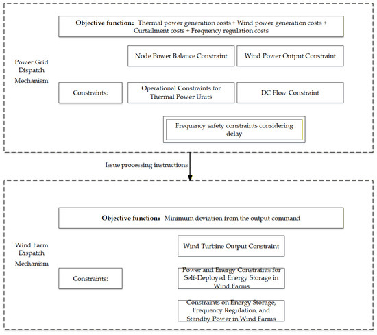
Figure 2.
Power Grid-Wind Farm Joint Dispatch Architecture Diagram.
3.1. Grid-Level Dispatch Mechanism
Power grid dispatch centers on economic efficiency and frequency security. By optimizing the start-stop operations of thermal power units, load allocation, and the utilization of wind farms’ frequency regulation capabilities, it constructs a comprehensive frequency security dispatch model that accounts for the response delay of wind turbines. The objective function of the dispatch model encompasses four components: thermal power operating costs, wind power operation and maintenance costs, curtailment costs, and frequency regulation reserve costs. Constraints include power balance, unit operational characteristics, wind power output limitations, power flow constraints, and frequency security constraints such as RoCoF, frequency level at nadir, and frequency level at quasi-steady-state constraint.
Building upon this foundation, the power grid dispatch model explicitly incorporates the impact of wind turbine frequency regulation time delay on system frequency dynamics by introducing a time-delay response model. This enhances the system’s resilience against low-inertia disturbances. Model outputs include power output plans for each unit and frequency regulation reserve capacity at every time step, with wind power frequency regulation request information transmitted to the wind farm dispatch to support next-level optimization.
3.2. Wind-Farm-Level Dispatch Mechanism
The wind-farm-level dispatch mechanism is designed for rapid and precise tracking of the power output targets received from the grid-level dispatch. Its primary objective is to minimize the deviation from the designated power curve. This is achieved by optimally coordinating the actual power output of the wind turbines with any on-site energy storage systems. A key secondary objective is to maintain sufficient headroom (or reserve capacity) to be able to provide the primary frequency regulation (PFR) service as requested by the system, ensuring the farm’s ability to participate in frequency support [35].
4. Mathematical Model of the Joint Dispatch Framework
4.1. Grid-Level Optimization Model
4.1.1. Objective Function
The objective of the grid-level optimization is to minimize the total system operating cost over the dispatch horizon, while ensuring frequency security through the constraints detailed in the following subsection. The total cost F1 is formulated as:
where F1 is the comprehensive operating cost of the power grid, C1 is the operating cost of thermal power units, C2 is the operating cost of wind power, C3 is the curtailment cost, C4 is the frequency regulation cost, T is the dispatch cycle, N is the total number of thermal power units, ai, bi, ci respectively are the consumption characteristic coefficients for the secondary, primary, and constant terms of thermal power unit I, ugi,t is the start/stop status of thermal power unit i at time t, Sgi is the start-stop cost of thermal power unit I, Nw is the number of wind farms, σw is the wind farm operation and maintenance cost coefficient, Ptargetw,t is the system’s target output for wind farm w at time t, cw is the curtailment cost coefficient for wind farm w, Pprew,t is the predicted output of wind farm w at time t, Δt is the scheduling step size, cpfrgi and cpfrw are the frequency regulation cost reserve coefficients for thermal power unit i and wind farm w, respectively, Ppfrgi,t and Ppfrw,t are the primary frequency regulation outputs of thermal power unit i and wind farm w at time t, respectively.
4.1.2. Constraints
The grid-level optimization is subject to the following constraints:
- (1)
- Power Balance Constraint
- (2)
- Thermal Unit Constraints
- (3)
- Wind Power Output Constraint
Wind power output at time t shall not exceed its forecasted output:
- (4)
- DC Power Flow Constraints
- (5)
- Frequency Security Constraints
The system must remain secure against the largest credible disturbance. This is enforced by the constraints derived in Section 2.2, specifically Equations (11), (16) and (19), which incorporate the impact of wind turbine FM delays.
4.2. Wind-Farm-Level Optimization Model
4.2.1. Objective Function
The primary objective at the wind-farm level is to minimize the deviation between the actual farm output and the target Ptargetw,t dispatched from the grid level. This is formulated as:
where PWw,t is the actual output of wind farm w at time t.
4.2.2. Constraints
- (1)
- Wind Turbine Output Constraintswhere PEww,t is the self-consumption energy output of wind farm w, uEww,t is the charge–discharge state of wind farm w’s self-consumption energy storage, MEw is a sufficiently large positive number.
- (2)
- Power and Energy Constraints for Self-Deployed Energy Storage in Wind Farms [26]where PEw,Nw is the rated output of wind farm w’s self-consumption energy storage system, SEww,t, SEww,0, and SEww,T are the SOC of wind farm w’s self-consumption energy storage at time t, initial time, and final time, respectively, EEw,Nw are the rated capacity of wind farm w’s self-consumption energy storage, η is the energy storage charging/discharging efficiency, Pcw,t and Pdw,t are the charging and discharging power of wind farm w’s self-sufficient energy storage, respectively, SEww,min and SEww,max are the minimum and maximum SOC of wind farm w’s self-sufficient energy storage, respectively, REw+w,t and REw-w,t are the positive and negative reserve capacity of wind farm w’s self-sufficient energy storage at time t, respectively.
- (3)
- Constraints on Energy Storage, Frequency Regulation, and Standby Power in Wind Farmswhere ξ+w and ξ−w are the positive and negative primary frequency regulation limiting coefficients of wind farms, respectively.
- (4)
- Wind Turbine Frequency Regulation Reserve Saturation Constraint
The primary frequency regulation power provided by a wind farm must not exceed its available headroom at any time. This constraint ensures that the wind farm maintains sufficient headroom to deliver the upward frequency regulation service when dispatched at Ptargetw,t.
where Ppfrw,t is the primary frequency regulation power from wind farm w at time t.
4.3. Joint Dispatch Process
The iterative process of the proposed joint dispatch framework is illustrated in Figure 3 and can be summarized as follows:
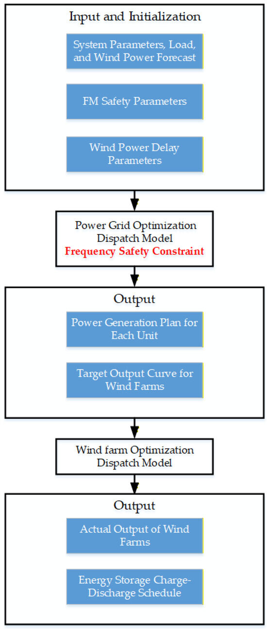
Figure 3.
Flowchart of the Joint Dispatch Mathematical Model.
Grid-Level Dispatch: The grid-level optimizer, using system-wide data and the proposed frequency security constraints, solves the optimization model described in Section 4.1. The solution provides the commitment and dispatch for thermal units, and, crucially, the target power output curve Ptargetw,t for each wind farm.
Wind-Farm-Level Dispatch: Each wind farm receives its target output curve Ptargetw,t. from the grid level. Its local controller then solves the wind-farm-level optimization model from Section 4.2. This internal optimization determines the optimal setpoints for individual wind turbines and the co-located ESS to track the target curve accurately while maintaining the required frequency regulation reserves.
This two-level process ensures that system-wide economic and security objectives are met at the grid level, while accounting for the practical capabilities and delayed responses of wind farms at the local level, thereby achieving coordinated and frequency-secure operation.
5. Case Study
5.1. System Parameters
This paper employs an enhanced IEEE 39-node system for simulation analysis, with the system topology diagram shown in Figure 4. G denotes thermal power units, while W represents wind power units. The system comprises six thermal power units and three wind farms, with specific parameters referenced in [26], parameters of thermal power units are shown in Table 1, wind farm parameters are shown in Table 2. System frequency regulation safety parameters and cost coefficients are referenced in [36]. The system load damping coefficient is 1%, the maximum frequency change rate limit is 0.25 Hz/s, the maximum frequency deviation limit is 0.2 Hz, and the steady-state frequency deviation limit is 0.1 Hz. The frequency regulation deadband time and deadband are 0.1 s and 0.033 Hz, respectively. The frequency regulation delay for wind units is set to 0.5 s, with a frequency regulation coefficient of 0.05. The frequency regulation delay for thermal units is set to 0.2 s, with a frequency deviation coefficient of 0.042. The inertia time constants for thermal units are 6.75 s, 6.4 s, 5.3 s, 5.3 s, 5.6 s, and 4.8 s, respectively. The inertia time constant for wind units is 8 s, and the maximum load disturbance power is set to 5%. The dispatch time step is 15 min. The predicted output curve for the wind farm is shown in Figure 5, and the load forecast curve is shown in Figure 6.
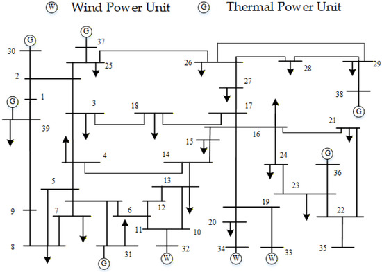
Figure 4.
Topology of the modified IEEE 39-bus test system.

Table 1.
Parameters of Thermal Power Units.
Table 2.
Parameters of Wind Farms.
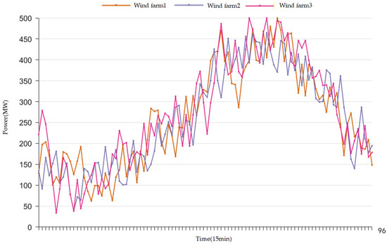
Figure 5.
Forecasted power output for the three wind farms.
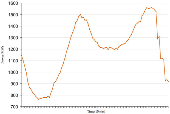
Figure 6.
System load forecast profile.
The proposed optimization models for both the grid-level and the wind-farm-level dispatch are implemented as Mixed-Integer Linear Programming (MILP) problems. The models are constructed using the YALMIP modeling toolbox in MATLAB R2023a. The resulting MILP problems are solved using the Gurobi Optimizer 10.0.1. All simulations were conducted on a computer equipped with an Intel i9-13980HX processor and 24 GB of RAM. Under this setting, all case study scenarios were solved to prove optimality within 3 to 5 min of computation time.
5.2. Grid-Level Dispatch Results and Analysis
To validate the effectiveness of the proposed grid-level dispatch model that incorporates wind turbine FM delays, three distinct scenarios are defined for comparative analysis:
- Scenario 1: The dispatch model includes the frequency security constraints derived in Section 2, which explicitly account for wind turbine FM delay;
- Scenario 2: The dispatch model includes frequency security constraints, but these constraints are based on traditional models that assume an ideal, instantaneous response from wind farms [26]. This scenario overlooks the FM delay;
- Scenario 3: The dispatch model minimizes cost without considering any frequency security constraints, representing a purely economic dispatch.
The peak-shaving outputs of each unit under the different dispatch scenarios are shown in Figure 7.
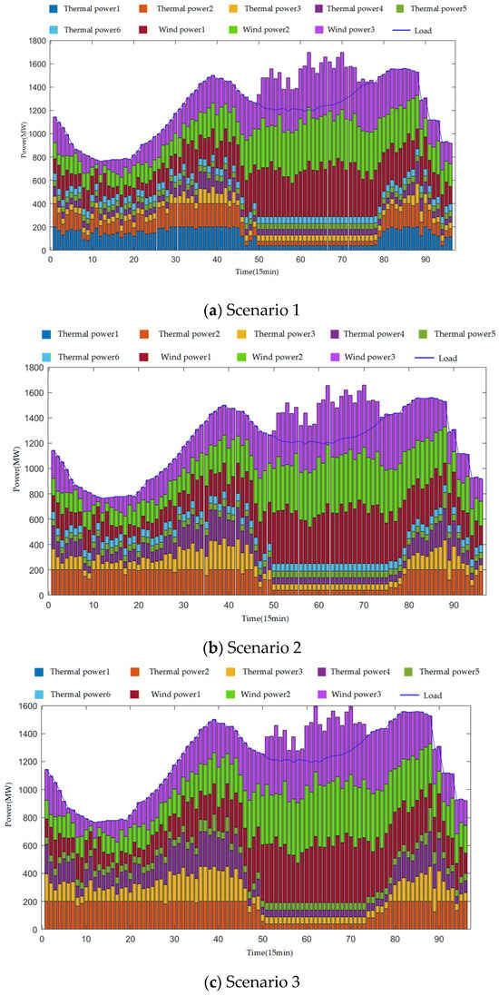
Figure 7.
Peak-shaving output of each unit under different scenarios.
Analysis of the simulation results in Figure 7 reveals that, although the total system load and wind power output forecasts remain consistent across the three dispatch scenarios, the dispatch models exhibit distinct differences in their activation strategies for thermal units due to varying approaches to handling frequency security constraints.
Figure 7a shows the method scheduling results for Scenario 1. The system commits more thermal units across more time periods to maintain sufficient online inertia and fast-response capacity, compensating for the delayed response from wind farms. Scenario 1 results indicate that due to response delays in wind turbine frequency regulation, the system prioritizes deploying thermal units with rapid response capabilities for frequency regulation and load support to ensure frequency safety metrics like RoCoF and frequency level at nadir remain within limits. Consequently, a higher number of thermal units are activated, sacrificing some economic efficiency to achieve stable frequency control and disturbance resistance. Figure 7b shows the method scheduling results for Scenario 2. Overestimating wind FM capability leads to a more economical but riskier schedule with fewer thermal units online, particularly during low-load periods such as time points 5–15. Figure 7c shows the method scheduling results for Scenario 3. Scenario 3 disregards the system’s frequency regulation safety requirements, with the optimization objective solely focused on minimizing costs. To further reduce operating expenses, the system reduces the number of activated thermal units without affecting total output, placing the system in an economically optimized state. However, this approach results in a severe shortage of potential frequency regulation capacity. When facing wind power frequency regulation delays, the system proactively introduces more conventional power sources with inertia and response capabilities to maintain safe frequency operation. Conversely, when frequency regulation capacity is “overestimated” or constraints are removed, the system may excessively pursue economic efficiency, potentially creating a gap in frequency regulation resources and threatening system security.
The frequency regulation outputs of each unit obtained from the dispatch results of Scenarios 1 and 2 are shown in Figure 8. Figure 8a shows the method frequency modulation results for Scenario 1. The model strategically allocates a larger share of the frequency regulation reserve to responsive thermal units to ensure reliable and immediate response despite wind power delays. Figure 8b shows the method frequency modulation results for Scenario 2. Compared to Scenario 1, this approach reduces the participation of thermal power units in frequency regulation support at certain times.
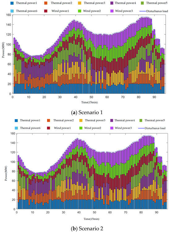
Figure 8.
Frequency regulation output of each unit under different scenarios.
Analysis of the simulation results in Figure 8 reveals that Scenario 1 mobilizes more thermal power units to participate in frequency regulation support at certain times compared to Scenario 2, thereby compensating for the gap in frequency regulation capacity caused by the delay in wind turbine frequency regulation.
Regarding system frequency security comparison, Scenario 1 outperforms other scenarios in both maximum system frequency deviation and RoCoF performance. Figure 9 illustrates the comparison of maximum system frequency deviations at each time point across all scenarios. The average values of system frequency security indicators for each scenario are summarized in Table 3. Scenario 1 incorporates frequency safety constraints accounting for wind turbine frequency regulation delays. The maximum deviation calculated using the maximum frequency deviation considering delays remains below 0.2 Hz, with the average maximum deviation also below 0.2 Hz, meeting the maximum frequency deviation limit constraint. Additionally, it achieves the lowest average RoCoF level. Scenario 2 employs traditional frequency safety constraints. The maximum deviation calculated by considering the maximum frequency deviation with delay exceeds 0.2 Hz at certain times, surpassing the maximum frequency deviation limit. The mean maximum frequency deviation approaches 0.2 Hz. Physically, although the control system detects frequency drops, it lags in executing active power adjustments, leading to increased maximum frequency deviation. Scenario 3, without frequency safety constraints, exhibits maximum frequency deviations exceeding 0.2 Hz during most time intervals, with the average maximum frequency deviation surpassing 0.2 Hz, resulting in frequency out-of-bounds conditions. In Figure 10, Scenario 1 exhibits a significantly lower frequency change rate than Scenarios 2 and 3 following initial disturbances, with more controllable fluctuation ranges, demonstrating superior capability in suppressing abrupt frequency changes. The system inertia values calculated for the three scenarios using Equation (10) are 17,720 MWs, 16,370 MWs, and 14,930 MWs, respectively, further confirming Scenario 1′s superior system stability.
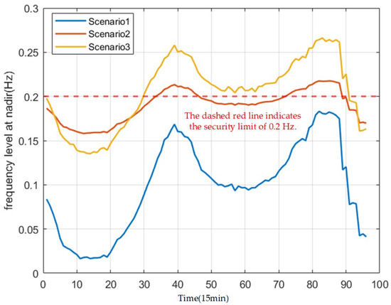
Figure 9.
Frequency Level at Nadir Comparison Chart.
Table 3.
System Frequency Security Metrics Comparison.
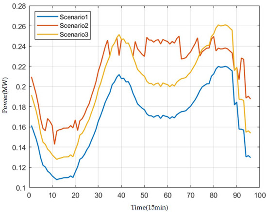
Figure 10.
ROCOF Comparison Chart.
By incorporating the frequency regulation delay characteristics of wind turbines into the dispatch process, Scenario 1 enhances resilience against low-inertia disturbances. Although the proposed strategy slightly increases operational costs, it significantly improves frequency security, prevents extreme control measures such as load shedding or unit tripping caused by frequency instability, avoids greater potential economic losses, and enhances the long-term security and stability of the power system. To quantitatively evaluate the comprehensive performance of the proposed method, Table 4 compares the key economic for the three scenarios. To ensure frequency security, the peak-shaving cost of the proposed method (Scenario 1) is 4% higher than that of Scenario 2, and 6% higher than the purely economic dispatch in Scenario 3. The frequency modulation cost of the proposed method (Scenario 1) is only 0.01% higher than that of Scenario 2. This cost increase is within an acceptable range for practical engineering. The security benefits gained from this economic cost are substantial. Compared to Scenario 2, Scenario 1 improves the average frequency nadir by 0.092Hz and reduces the average RoCoF by 0.048 Hz/s. Compared to Scenario 3, Scenario 1 improves the average frequency nadir by 0.107Hz and reduces the average RoCoF by 0.031 Hz/s. Furthermore, Scenario 1 will not experience frequency overshoot.
Table 4.
Economic Comparison.
5.3. Analysis of Wind Farm Dispatch Results
Each wind farm conducts on-site dispatch based on the output curves generated according to the dispatch results from Scenario 1. The resulting output curves for each wind farm and its self-allocated energy storage are shown in Figure 11, while the reserve curves for each wind farm are presented in Figure 12.
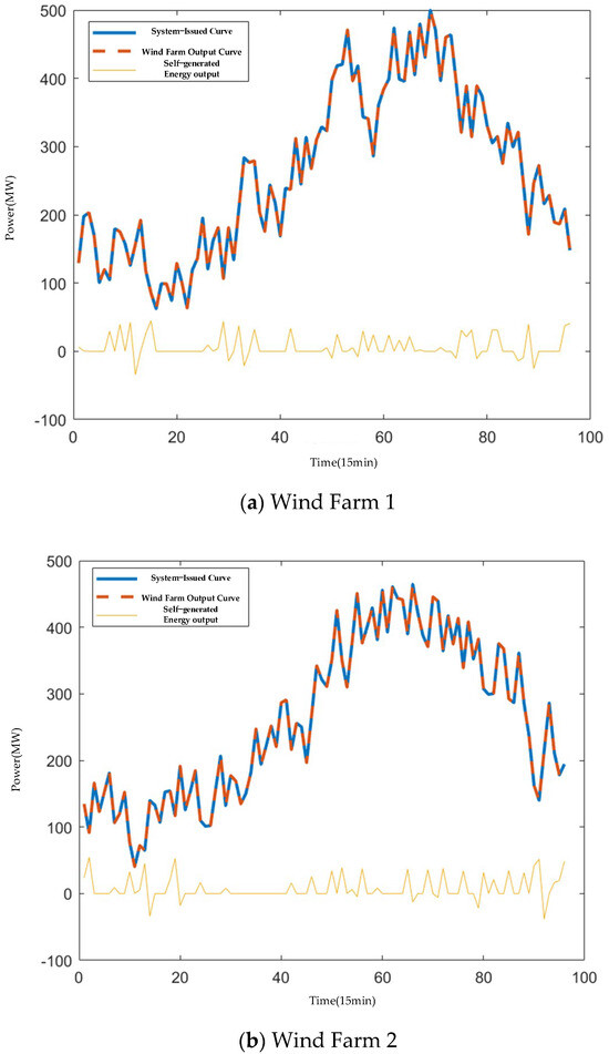
Figure 11.
Output Curves for Each Wind Farm and Self-generated Energy Storage.
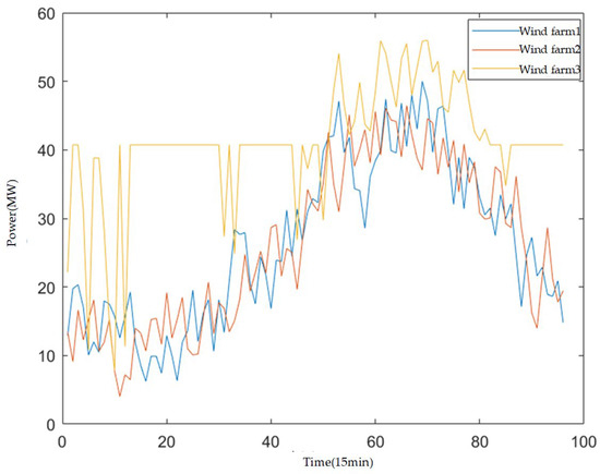
Figure 12.
Standby Power Curves for Each Wind Farm.
As shown in Figure 10, the output curves of each wind farm effectively track the target outputs issued by the system. Simultaneously, the flexible charging and discharging of energy storage compensates for the impact of wind power output fluctuations. The results in Figure 12 indicate that each wind farm maintains sufficient reserve power, providing robust support for frequency regulation requirements.
5.4. Sensitivity Analysis
To evaluate the robustness of the proposed joint dispatch model and investigate the impact of key parameters on system frequency security, a sensitivity analysis is conducted based on the Scenario 1 setup. The critical parameters under study include the wind turbine frequency regulation delay (τ) and the frequency regulation deadband time.
5.4.1. Sensitivity Studies for Delay τ
Wind turbine frequency modulation delay is the core parameter of this model. We will vary τ from 0.5 s to 1.0 s in increments of 0.1 s. The comparison results for frequency level at nadir average is shown in Table 5 below.
Table 5.
The Effect of τ on Frequency Level at Nadir Average.
The frequency level at nadir average monotonically increases with τ, while the system frequency margin decreases as τ increases. When τ is 1 s, frequency level at nadir average reaches as high as 0.133 Hz, an increase of 0.035 Hz compared to when τ is 0.5 s.
5.4.2. Sensitivity Studies for Frequency Regulation Deadband Time
Deadband time determines the speed at which frequency-modulated units respond to disturbances. This paper tested scenarios with deadband time values of 0.05 s, 0.1 s, and 0.15 s. The impact on system frequency security is shown in Table 6.
Table 6.
The Effect of deadband time on Frequency Level at Nadir Average.
A larger deadband delays the activation of frequency support, leading to a deeper frequency nadir and a later arrival at that nadir. When deadband time reaches 0.2 s, frequency level at nadir average is 0.102 Hz, an increase of 0.004 Hz compared to when deadband time is 0.1 s. Time of arrival at frequency level at nadir average is 2.522 s, an increase of 0.046 s compared to when frequency level at nadir average is 0.1 s.
The sensitivity analysis verifies that the proposed joint dispatch model is robust to variations in key parameters.
6. Conclusions
This paper has presented a joint dispatch model for power grids and wind farms that explicitly incorporates the frequency regulation delay of wind turbines into system-wide frequency security constraints. The key conclusions derived from this work are summarized as follows:
(1) Explicitly modeling the FM delay of wind turbines and deriving corresponding frequency security constraints provides a crucial theoretical basis for achieving frequency-stable dispatch in systems with high wind penetration. Neglecting this delay leads to an underestimation of the system’s actual frequency deviation and RoCoF. The grid-level dispatch results confirm that the proposed delay-aware strategy significantly improves frequency security metrics—notably reducing the frequency nadir and RoCoF—with only a minor impact on operational economics, thereby effectively enhancing system stability.
(2) The case study provides quantitative evidence of the method’s efficacy. Compared to a traditional dispatch that ignores FM delays, the proposed model reduces the average frequency nadir by 0.092 Hz and the average RoCoF by 0.048 Hz/s, while increasing the peak-shaving cost by merely 4%. This demonstrates a favorable trade-off where substantial gains in frequency security are achieved at a modest economic cost.
(3) The results from the wind-farm-level dispatch demonstrate that wind farms can accurately track the power setpoints commanded by the grid-level optimizer. Furthermore, by optimally coordinating wind turbines and energy storage, the farms can maintain sufficient reserve capacity to reliably serve as primary frequency regulation resources, thereby fulfilling their role in ensuring overall system security.
Despite the promising results, this study has limitations that suggest valuable directions for future research. First, the model assumes a fixed, pre-determined delay value for all wind turbines, which may not capture the heterogeneity and stochastic nature of actual delays. Future work could investigate data-driven or stochastic models for delay characterization. Second, the model was validated on a single, modified test system. Its performance and scalability should be further assessed on larger, more realistic networks with diverse generation mixes. Finally, extending the framework to account for uncertainties in wind power and load forecasts via stochastic or robust optimization techniques would enhance its practical applicability.
Author Contributions
Conceptualization, J.H., Y.Z., Y.L., W.L. and Y.S.; methodology, J.H., Y.Z. and Y.L.; software, J.H.; Validation, J.H.; Investigation, J.H. and Y.L.; Resources, J.H.; formal analysis, J.H.; data curation, J.H.; writing—original draft preparation, J.H., Y.Z. and Y.L.; writing—review and editing, J.H., Y.Z.,Y.L., W.L. and Y.S.; Visualization, J.H.; Supervision, J.H., Y.Z. and Y.L.; Project Administration, J.H., Y.Z. and Y.L.; Funding Acquisition, Y.Z. and Y.L. All authors have read and agreed to the published version of the manuscript.
Funding
This research was funded by National Key R&D Program of China (Grants No. 2024YFB3411000). The support is greatly appreciated.
Data Availability Statement
The data that support the findings of this study are available from the corresponding author upon reasonable request.
Conflicts of Interest
Authors Wenguang Lin and Yanping Sun were employed by the company Goldwind Sci & Tech Co., Ltd. The remaining authors declare that the research was conducted in the absence of any commercial or financial relationships that could be construed as a potential conflict of interest.
Nomenclature
| Symbol | |
| t, T | Time index and total scheduling periods |
| i, g, G | Index, generic index, and set of thermal units |
| w, W | Index and set of wind farms |
| n, N | Index and set of nodes |
| L, ΩLTn, ΩLFn | Transmission line, set of lines to/from node n |
| ai, bi, ci | Fuel cost coefficients of thermal unit i ($/(MW)2, $/MW, $) |
| Sgi | Startup/shutdown cost of thermal unit i ($) |
| Pmaxgi, Pmingi | Maximum/minimum power output of thermal unit i (MW) |
| rupgi, rdowngi | Ramp-up/ramp-down limits of thermal unit i (MW/h) |
| hg, hw | Inertia time constant of thermal unit g/wind farm w (s) |
| Sg, Sw | Installed capacity of thermal unit g/wind farm w (MW) |
| σw | O&M cost coefficient of wind farm w ($/MW) |
| cw | Curtailment penalty cost coefficient of wind farm w ($/MW) |
| cpfrgi, cpfrw | PFR reserve cost of thermal unit i/wind farm w ($/MW) |
| Pprew,t | Forecasted power output of wind farm w at time t (MW) |
| f0 | System rated frequency (Hz) |
| D | Load damping coefficient (p.u.) |
| τ | FM delay time of wind turbines (s) |
| tDB | FM deadband time (s) |
| RW, RG | Maximum PFR power of wind farm/thermal unit (MW) |
| Td | Duration of primary frequency response (s) |
| RoCoFmax | Maximum allowable Rate of Change of Frequency (Hz/s) |
| Δfmax | Maximum allowable frequency deviation (Hz) |
| Δfssmax | Maximum allowable quasi-steady-state frequency deviation (Hz) |
| XL | Reactance of line L (p.u.) |
| Power transmission limit of line L (MW) | |
| PEw,Nw | Rated power capacity of wind farm w’s energy storage (MW) |
| EEw,Nw | Rated energy capacity of wind farm w’s energy storage (MWh) |
| η | Charging/discharging efficiency of energy storage |
| ξ+w, ξ−w | Positive/Negative PFR limiting coefficients of wind farm w |
| Pgi,t | Power output of thermal unit i at time t (MW) |
| Ptargetw,t | System-dispatched target output for wind farm w at time t (MW) |
| PWw,t | Actual power output of wind farm w at time t (MW) |
| Ppfrgi,t, Ppfrw,t | PFR reserve from thermal unit i/wind farm w at time t (MW) |
| M(t), H(t) | Total system inertia at time t (MWs) |
| ΔPW(t) | the power output of the wind turbine during the primary frequency response at time t (MW) |
| Δf(t) | the frequency deviation of the system at time t (Hz) |
| the load disturbance at time t (MW) | |
| θn,t | Voltage phase angle at node n and time t (rad) |
| PL,t | Power flow on line L at time t (MW) |
| PEww,t | Net discharge power of wind farm w’s energy storage at time t (MW) |
| SEww,t | State of Charge (SOC) of wind farm w’s energy storage at time t (MWh) |
| Pcw,t, Pdw,t | Charging/Discharging power of wind farm w’s energy storage (MW) |
| ugi,t | On/Off status of thermal unit i at time t {0, 1} |
| uEww,t | Charge–Discharge state of wind farm w’s energy storage {0, 1} |
References
- Xie, K.C. China’s Energy Development for 2035: Strategic Thinking and Suggestions. Strateg. Study CAE 2022, 24, 1–7. [Google Scholar] [CrossRef]
- Li, L.C.; Rao, H.; Xu, A.D.; Guo, X.; Bai, H. Strategic Research on China Energy Technology Revolution System. Strateg. Study CAE 2018, 20, 1–8. [Google Scholar] [CrossRef]
- Global Wind Energy Council. Global Wind Report 2023. Available online: https://www.enertechnos.com/wp-content/uploads/2023/12/GWEC-2023-Report.pdf (accessed on 7 November 2025).
- Li, Y.; Wu, W.; Zhang, Y.; Zheng, M.; Lou, Y.; Yu, L.; Cai, Y. Mechanism of inertia loss and evaluation of inertia level in power systems with large scale new energy access. South. Energy Constr. 2024, 11, 132–139. [Google Scholar]
- Roy, N.K.; Islam, S.; Podder, A.K.; Roy, T.K.; Muyeen, S.M. Virtual Inertia Support in Power Systems for High Penetration of Renewables—Overview of Categorization, Comparison, and Evaluation of Control Techniques. IEEE Access 2022, 10, 129190–129216. [Google Scholar] [CrossRef]
- An, Y.; Zhang, Y.; Lin, J.; Yi, Y.; Fan, W.; Cai, Z. Ultra-Short-Term Power Prediction of Large Offshore Wind Farms Based on Spatiotemporal Adaptation of Wind Turbines. Processes 2024, 12, 696. [Google Scholar] [CrossRef]
- Xiao, H.Y.; Zhong, K.H.; Fan, W.; Yi, Y.Q.; Huo, J.X.; Zhang, Y.J. Reactive power optimization control interval setting for offshore wind farm grid connection points. Power Syst. Prot. Control. 2025, 53, 23–32. [Google Scholar]
- Guan, L.; Yao, J. Dynamic coupling and cooperative control for multi-paralleled doubly fed induction generator wind farms during symmetrical low voltage ride-through in a weak grids. Prot. Control Mod. Power Syst. 2024, 9, 112–125. [Google Scholar] [CrossRef]
- Zhao, C.; Sun, D.; Zhang, X.; Ke, W.; Hu, B.; Nian, H. A Two-Stage Power Distribution Scheme of Multiple Wind Farms Participating in Primary Frequency Regulation. IEEE Trans. Power Syst. 2023, 38, 5009–5021. [Google Scholar] [CrossRef]
- Li, K.; Guo, H.; Feng, C.; Yu, S.; Tang, Y. Modeling strategic behaviors of renewable-storage system in low-inertia power system. Prot. Control Mod. Power Syst. 2025, 10, 28–40. [Google Scholar] [CrossRef]
- Hosseini, S.A.; Fotuhi-Firuzabad, M.; Dehghanian, P.; Lehtonen, M. Coordinating Demand Response and Wind Turbine Controls for Alleviating the First and Second Frequency Dips in Wind-Integrated Power Grids. IEEE Trans. Ind. Inform. 2024, 20, 2223–2233. [Google Scholar] [CrossRef]
- Huang, J.; Xu, Y.; Ghias, A.M. Wind Power Plant Dispatch for Power Grid Frequency Dynamics Improvement: A Surrogate Model-Based Method. IEEE Trans. Power Syst. 2025, 40, 3261–3275. [Google Scholar] [CrossRef]
- Dong, W.; Shi, Z.M.; Zhang, X.L.; Chen, Z.L.; Su, J.H. Frequency Response Model and Application of Power System Considering the Frequency Regulation Delay of Renewable Energy Station. Proc. CSEE 2025, 45, 4657–4668. [Google Scholar]
- Chen, X.Y.; Liu, C.H.; Yang, P.W.; Bao, Y.F.; Feng, X. Measurement and Analysis of Primary Frequency Control in Wind Farm of East Inner Mongolia. Northeast. Electr. Power Technol. 2024, 45, 6–11+17. [Google Scholar]
- Liu, C.H.; Bao, Y.F.; Chen, X.Y.; Chen, H. Measurement and Analysis of Active Frequency Support Strategy for Wind Storage Joint System. Northeast. Electr. Power Technol. 2024, 42, 17–23. [Google Scholar]
- Zhang, M.; Li, S.L.; Li, D.; Qin, S.Y.; Zhang, H.P. Measurement and Analysis of Wind Power Inertia Response and Primary Frequency Regulation Characteristics in Northeast China Power Grid. Power Syst. Technol. 2022, 46, 1624–1631. [Google Scholar]
- Miao, F.L.; Li, S.L.; Qin, S.Y.; He, J.; Zhang, J. Simulation Analysis and Application of Wind Farm Based on Multi-controllers Hardware-in-the-loop Simulation technologies. Acta Energiae Solaris Sin. 2023, 44, 451–460. [Google Scholar]
- Zhang, N.; Zhang, Z.; Xu, Z. A Coordinated Adaptive SMC Method for Frequency Regulation Control in Power Systems with Multiple Wind Farms. IEEE Trans. Sustain. Energy 2025, 16, 1806–1815. [Google Scholar] [CrossRef]
- Sun, M.; Min, Y.; Xiong, X.; Chen, L.; Zhao, L.; Feng, Y.; Wang, B. Practical Realization of Optimal Auxiliary Frequency Control Strategy of Wind Turbine Generator. J. Mod. Power Syst. Clean Energy 2022, 10, 617–626. [Google Scholar] [CrossRef]
- Harag, N.; Imanaka, M.; Kurimoto, M.; Sugimoto, S.; Bevrani, H.; Kato, T. Autonomous Dual Active Power-frequency Control in Power System with Small-scale Photovoltaic Power Generation. J. Mod. Power Syst. Clean Energy 2022, 10, 941–953. [Google Scholar] [CrossRef]
- Wang, M.; Guo, J.; Ma, S.; Zhang, X.; Wang, T.; Luo, K. A Novel Decentralized Frequency Regulation Method of Renewable Energy Stations Based on Minimum Reserve Capacity for Renewable Energy-Dominated Power Systems. IEEE Trans. Power Syst. 2024, 39, 3701–3714. [Google Scholar] [CrossRef]
- Liu, Y.; Sun, K.; Zhu, L.; Qu, L.; Li, K.-J. PCC-COI Frequency Based Auxiliary Frequency Control Strategy for Windfarm Frequency Support Improvement. In Proceedings of the 2023 IEEE Industry Applications Society Annual Meeting (IAS), Nashville, TN, USA, 29 October–2 November 2023; pp. 1–8. [Google Scholar]
- Teng, F.; Trovato, V.; Strbac, G. Stochastic scheduling with inertia-dependent fast frequency response requirements. In Proceedings of the 2016 IEEE Power and Energy Society General Meeting (PESGM), Boston, MA, USA, 17–21 July 2016; p. 1. [Google Scholar]
- Liu, X.Y.; Zhang, L.H.; Gu, X.P.; Li, H.B.; Zhong, W.Z.; Li, Z.H. Day Ahead Dispatching Model of Low Inertia Power Grid Considering Security Constraints of Peak Shaving and Frequency Regulation. Proc. CSEE 2025, 45, 8390–8402. [Google Scholar]
- Wang, T.; Wang, T.T.; Liu, R.; Li, G.Y.; Qi, X.G.; Miao, S.H. Unit Commitment Model of High Proportion Wind Power System Considering Dynamic Frequency Response Constraints. High Volt. Eng. 2021, 47, 3463–3479. [Google Scholar]
- Hu, M.K.; Zhang, G.H.; Li, F.T.; Xie, C.; Yin, C.Y. A Two-stage Optimal Scheduling Method for High Penetration Level of Wind Power System Considering Frequency Security and Peaking Demand. Power Syst. Technol. 2025, 49, 4365–4375. [Google Scholar]
- Qi, X.; Liu, J.; Zhang, W.; Deng, H. Nonlinear Real-Time Distributed Optimal Control for Frequency Regulation of Cyber–Physical Power Systems. IEEE Trans. Ind. Electron. 2025, 72, 9139–9149. [Google Scholar] [CrossRef]
- Zhang, Y.; Xie, Y.; Cai, S.; Wu, Q.; Zhu, H.; Xiang, Z. Coordinated Control of Grid-Forming Wind Turbines and Grid-Forming Energy Storage Systems for Power System Restoration. IEEE Trans. Sustain. Energy 2025, 16, 2812–2827. [Google Scholar] [CrossRef]
- Zhao, H.; Zong, Q.; Zhou, H.; Yao, W.; Sun, K.; Zhou, Y.; Wen, J. Frequency-Voltage Active Support Strategy for Hybrid Wind Farms Based on Grid-Following and Grid-Forming Hierarchical Subgroup Control. CSEE J. Power Energy Syst. 2025, 11, 65–77. [Google Scholar]
- D’Arco, S.; Sanchez-Acevedo, S.; Suul, J.A. Multi-Hardware-in-the-Loop Laboratory Testing of Power Converters and Intelligent Electronic Devices for Large-Scale Power System Applications. IEEE Open J. Power Electron. 2024, 5, 1520–1533. [Google Scholar] [CrossRef]
- Gupta, S.; Shukla, A.; Abusara, M. Integrated Co-Simulation and Hardware-in-the-Loop Testing for Microgrid. IEEE Trans. Ind. Electron. 2025, 72, 9082–9094. [Google Scholar] [CrossRef]
- Zhang, Z.; Zhou, M.; Wu, Z.; Liu, S.; Guo, Z.; Li, G. A Frequency Security Constrained Scheduling Approach Considering Wind Farm Providing Frequency Support and Reserve. IEEE Trans. Sustain. Energy 2022, 13, 1086–1100. [Google Scholar] [CrossRef]
- He, H.; Cai, X.; Su, Y.; Zhang, X.; Zhang, N.; Ci, S.; Zhou, Y.; Kang, C. Impact of Communication Time Delay in a 5G Network on Frequency Regulation Performance of a High Renewable Energy Penetrated Power System. IEEE Internet Things J. 2024, 11, 24376–24388. [Google Scholar] [CrossRef]
- Nguyen, N.; Almasabi, S.; Bera, A.; Mitra, J. Optimal Power Flow Incorporating Frequency Security Constraint. IEEE Trans. Ind. Appl. 2019, 55, 6508–6516. [Google Scholar] [CrossRef]
- Zhao, W.; Xu, P.; Li, F.; Pan, Y.; Pei, L.; Wang, T. Transient Frequency Coordinated Control Strategy for Wind Farm Augmented with Energy Storage. IEEE Trans. Ind. Appl. 2025, 61, 5501–5512. [Google Scholar] [CrossRef]
- Wang, J.; Miao, S.; Wang, T.; Yao, F.; Tan, H.; Chen, C. Multi-level optimal dispatch strategy for a high proportion of wind power system considering the wind power ramping limit and frequency security constraints. Power Syst. Prot. Control 2025, 53, 135–146. [Google Scholar]
Disclaimer/Publisher’s Note: The statements, opinions and data contained in all publications are solely those of the individual author(s) and contributor(s) and not of MDPI and/or the editor(s). MDPI and/or the editor(s) disclaim responsibility for any injury to people or property resulting from any ideas, methods, instructions or products referred to in the content. |
© 2025 by the authors. Licensee MDPI, Basel, Switzerland. This article is an open access article distributed under the terms and conditions of the Creative Commons Attribution (CC BY) license (https://creativecommons.org/licenses/by/4.0/).