Article

Research on Load Forecasting Based on Bayesian Optimized CNN-LSTM Neural Network

1
Marketing Service Center, State Grid Qinghai Electric Power Company, Xining 810016, China
2
State Grid Qinghai Electric Power Company, Xining 810016, China
3
School of Energy and Electrical Engineering, Qinghai University, Xining 810016, China
*
Author to whom correspondence should be addressed.
Energies 2025, 18(23), 6217; https://doi.org/10.3390/en18236217
Submission received: 29 October 2025 / Revised: 18 November 2025 / Accepted: 25 November 2025 / Published: 27 November 2025

Abstract

With the high penetration of renewable energy integration and massive user participation in electricity markets, traditional short-term load forecasting methods exhibit limitations in both adaptability and prediction accuracy. There is an urgent need to explore forecasting models that better accommodate the characteristics of new power systems to ensure the accuracy of load forecasting results. To address issues such as high feature dimensions and weak correlations in historical data, and to fully exploit the temporal dependencies in load data, this paper proposes a short-term power load forecasting method based on a Bayesian-optimized Convolutional Neural Network–Long Short-Term Memory (CNN-LSTM) model. Using typical industrial and agricultural load data from a region in Qinghai Province as training data, experimental results demonstrate that the hybrid forecasting model achieves superior performance compared to standalone LSTM and CNN-LSTM algorithms.

1. Introduction

1.1. Background and Significance

With the acceleration of global industrialization and growing energy demand, society faces increasingly severe challenges stemming from the over-reliance on fossil fuels, including the continuous depletion of non-renewable resources and worsening environmental pollution [1]. In response, countries worldwide are actively promoting a transition towards renewable energy-dominated power systems as a key strategy to mitigate environmental pollution and combat climate change. However, as the proportion of intermittent clean energy sources such as wind and solar power expands within the power structure, their large-scale integration introduces significant volatility and uncertainty into grid operations, posing substantial challenges to the safety and stability of power systems [2]. In this context, accurate load forecasting plays a crucial role in maintaining the reliable operation of the power grid. Enhancing the precision of load prediction and strengthening the capacity for optimized power system dispatch have become an essential task [3].

1.2. Literature Review

Electric load forecasting is a critical component in power system planning, operation, and dispatch. Its accuracy directly impacts the rationality of generation scheduling, the economic efficiency of grid operation, and the reliability of power supply quality. Load data exhibits significant temporal dependencies, seasonal variations, and periodic fluctuations. Simultaneously, it is susceptible to interference from multiple uncertain factors such as temperature changes, holiday effects, and complex meteorological conditions. These characteristics cause load profiles to demonstrate highly nonlinear and stochastic behavior, posing significant challenges for achieving accurate electric load forecasting [4].
Based on the forecasting time horizon, electric load forecasting is generally categorized into short-term, medium-term, and long-term forecasting [5,6,7]. Among these, Short-Term Load Forecasting (STLF), which covers a period from several hours to one week, plays a pivotal role in real-time grid dispatch, unit commitment decisions, electricity market trading, and ensuring stable system operation [8]. With the increasing penetration of renewable energy sources like wind and photovoltaic power in modern power systems, coupled with the large-scale integration of new types of loads such as electric vehicles, the spatiotemporal coupling characteristics of loads are becoming increasingly complex. This evolution places higher demands on forecasting techniques.
Early methods for short-term load forecasting primarily fall into two categories: one based on statistical models, such as time series methods [9] and linear regression, and the other on machine learning algorithms, such as Support Vector Machines (SVMs) [10], Random Forests, and XGBoost [11]. Among them, time series methods treat the collected load data as a predictable time series, utilizing historical data as a foundation to construct models that predict future trends in the power load sequence, thereby achieving load forecasting. Reference [12] employed the ARIMA model to identify and fit building load data, and introduced a metabolic GM(1,1) improved model to correct its residual subsequence, thus constructing a combined ARIMA-GM forecasting model incorporating residual correction to enhance the prediction accuracy for building loads.
Reference [13] first used the F-test to determine whether the dataset could linearly characterize the load, then applied the t-test to analyze the significance of the linear relationship between feature vectors and the load, eliminating those with weaker linear relationships. Finally, a concise linear regression model for load forecasting was established, significantly improving computational efficiency. Such methods are simple in structure, fast in computation, and possess good extrapolation capabilities. However, they rely heavily on the quality of historical data, struggle to capture the nonlinear dynamics of loads, and their initialization process often depends on expert experience, resulting in limited prediction accuracy.
Traditional machine learning algorithms, owing to their superior performance in time series forecasting, have been widely applied in load prediction. Support Vector Machines exhibit strong generalization ability and often perform well in most scenarios of power load forecasting [14]. Reference [15] proposed a power load forecasting method based on an improved SVM, introducing an enhanced SVM algorithm to construct a load forecasting model. Random Forest is a self-learning algorithm based on decision trees, usable for both regression and classification, and is widely used in load forecasting. Reference [16] used the Random Forest algorithm to extract features, then used the extracted features as input for a neural network, and finally corrected the prediction results using rough set theory. Feature selection via Random Forest significantly improved prediction accuracy. Although the Random Forest algorithm performs well in relevant feature selection, it struggles to deeply mine nonlinear characteristics of loads and is currently mainly applied in the feature selection stage of load forecasting. XGBoost, an improvement over Gradient Boosting Decision Trees (GBDTs), is a tree-based Boosting ensemble learning algorithm [17]. To address the limitation of conventional feature selection methods in effectively measuring nonlinear correlations between features, Reference [18] proposed a load forecasting method based on an improved Extreme Gradient Boosting (XGBoost) model with optimal feature combination. Reference [19], aiming to tackle the challenges of feature selection and generalization capability improvement in building load forecasting, proposed a load feature screening method based on XGBoost–Neural Network. This method uses XGBoost to train processed data and employs the Mean Absolute Percentage Error (MAPE) evaluation metric to determine the optimal feature subset, thereby improving model accuracy and generalization.
Although traditional machine learning methods represent an advancement over statistical models, they still exhibit significant limitations when applied to typical industrial and agricultural load forecasting. Firstly, model performance heavily relies on complex manual feature engineering. Industrial and agricultural loads are strongly influenced by domain-specific factors such as production processes, scheduling strategies, and irrigation cycles, making the quantification and construction of relevant features difficult and costly. Secondly, these methods have a limited capacity for capturing long-term temporal dependencies, making it challenging to effectively model complex nonlinear relationships, such as the time-lag effect of effective precipitation on irrigation load. Furthermore, when faced with multi-modal load distributions and sharp fluctuations caused by production seasonality, holidays, or extreme weather, the generalization ability and robustness of these models are often insufficient, leading to significant prediction errors, particularly at transition points between different load patterns.
The rapid advancement of artificial intelligence in recent years has significantly propelled progress in deep learning-based power load forecasting methods, prompting extensive exploration of various innovative model architectures and optimization strategies.
In the domain of recurrent neural networks (RNNs) and their enhanced architectures, Reference [20] developed a multi-scale RNN incorporating residual connections. This architecture employs stacked RNN layers, each utilizing dilated convolutional kernels with different dilation rates, enabling the parallel extraction of multi-scale temporal features from power load data. The residual connection mechanism facilitates feature fusion between adjacent layers, effectively enhancing the accuracy of short-term load forecasting. Regarding fundamental RNN units, Long Short-Term Memory (LSTM) networks and Gated Recurrent Units (GRUs) have demonstrated exceptional performance in sequence modeling tasks due to their unique gating mechanisms. Reference [21] constructed an LSTM-based load forecasting model using the TensorFlow framework, validating its effectiveness in handling temporal dependencies. Reference [22] employed a GRU combined with a stacked autoencoder for feature extraction and reconstruction. Experimental results indicated that this hybrid method surpassed Support Vector Machines and basic LSTM models in prediction accuracy.
Regarding hybrid CNN-RNN models and attention mechanisms, Reference [23] proposed a CNN-GRU forecasting framework integrated with an attention mechanism. This model first utilizes a CNN module composed of one-dimensional convolutional and pooling layers to extract local dynamic high-dimensional features from the load sequence. Subsequently, the extracted features are reorganized according to time steps and fed into a GRU for temporal modeling. Finally, the attention mechanism adaptively calculates the weights for the hidden state at each time step, with the weighted fusion result serving as the final prediction output. Such hybrid models aim to synergistically leverage the strengths of CNNs in local feature extraction and RNNs in modeling long-term dependencies.
In the field of signal decomposition and feature engineering, Reference [24] introduced a hybrid forecasting model based on Empirical Mode Decomposition (EMD) and CNN-LSTM. This method first applies EMD to decompose the original load sequence into multiple Intrinsic Mode Functions (IMFs). It then uses CNNs to extract spatial features from each component, and finally employs an LSTM network for temporal modeling and prediction output. This approach enhances forecasting stability.
Although these deep learning models demonstrate powerful feature extraction and temporal modeling capabilities, their predictive performance remains highly dependent on the configuration of key hyperparameters [25], such as learning rate, number of iterations, and convolution kernel size. These parameters constitute a high-dimensional and complex search space, while model training typically involves substantial computational costs. Consequently, developing efficient and automated hyperparameter optimization strategies has become particularly crucial.
In power load forecasting, model performance is highly dependent on hyperparameter configuration, which itself constitutes a complex, high-dimensional optimization problem. Traditional methods like grid search are simple and intuitive but suffer from exponentially increasing computational costs as parameters grow. Random search improves efficiency to some extent by sampling hyperparameters randomly, but its undirected strategy struggles to stably approximate the global optimum under limited computational resources [26,27]. Heuristic algorithms like Genetic Algorithms [28] and Particle Swarm Optimization [29], despite their global search potential, involve complex parameter tuning, exhibit unpredictable convergence behavior, and are prone to becoming trapped in local optima.

1.3. Main Contributions

Currently, Bayesian optimization (BO) has gained significant popularity in tuning computationally expensive deep learning models due to its efficient search capability enabled by probabilistic surrogate models, particularly for complex black-box functions such as load sequences. To address the limitations of existing hyperparameter optimization methods in terms of efficiency and accuracy, this study proposes an automatic hyperparameter tuning approach based on Bayesian optimization for a hybrid CNN-LSTM model. The method first applies the K-means algorithm to perform cluster analysis on load data, aiming to identify inherent patterns. The clustering results are then fed into a CNN-LSTM hybrid architecture, where the CNN extracts spatial features from the input data, and the LSTM further captures temporal dependencies, thereby enabling joint spatiotemporal feature modeling. On this basis, a Bayesian optimization algorithm is introduced to adaptively search for optimal values of key hyperparameters, such as learning rate, number of iterations, and convolution kernel size. By establishing a surrogate model and an acquisition function mechanism, the search process is transformed into an efficient active learning procedure, which significantly improves sample efficiency and convergence performance under limited computational resources. To validate the effectiveness of the proposed method, empirical studies are conducted using actual industrial and agricultural load data from a region in Qinghai. Simulation results demonstrate that the Bayesian optimization-based CNN-LSTM model significantly enhances the accuracy and robustness of short-term power load forecasting, indicating considerable value for engineering applications.

2. Model Architecture and Components

2.1. Convolutional Neural Network

A Convolutional Neural Network (CNN) is a type of feedforward neural network [30] widely used in image recognition and visual tasks, making it one of the core models in deep learning. Through its hierarchical structure comprising convolutional layers, pooling layers, and fully connected layers, it automatically extracts local features from input data, progressively compresses information, reduces redundancy, and enhances generalization capability. Compared to traditional fully connected neural networks, CNNs demonstrate superior performance when processing data with a grid-like structure. A typical CNN primarily consists of the following components: convolutional layers, pooling layers, and fully connected (FC) layers, as illustrated in Figure 1.
Through the stacking of multiple convolutional and pooling layers, low-level input features are progressively transformed into high-level abstract feature representations. The alternating action of convolutional and pooling layers can effectively reduce the size of feature maps while increasing feature diversity and robustness. This layer-by-layer abstraction process enables the network to learn increasingly abstract and advanced features. The computational formula is as follows:
M j N = f M j N 1 c j N + b j N
In the formula: f(x) is the activation function implemented using the ReLU function; M j N represents the j-th feature map in the N-th convolutional layer; c j N denotes the j-th convolutional kernel in the N-th convolutional layer; and b j N is the additive bias term.

2.2. Long Short-Term Memory Network

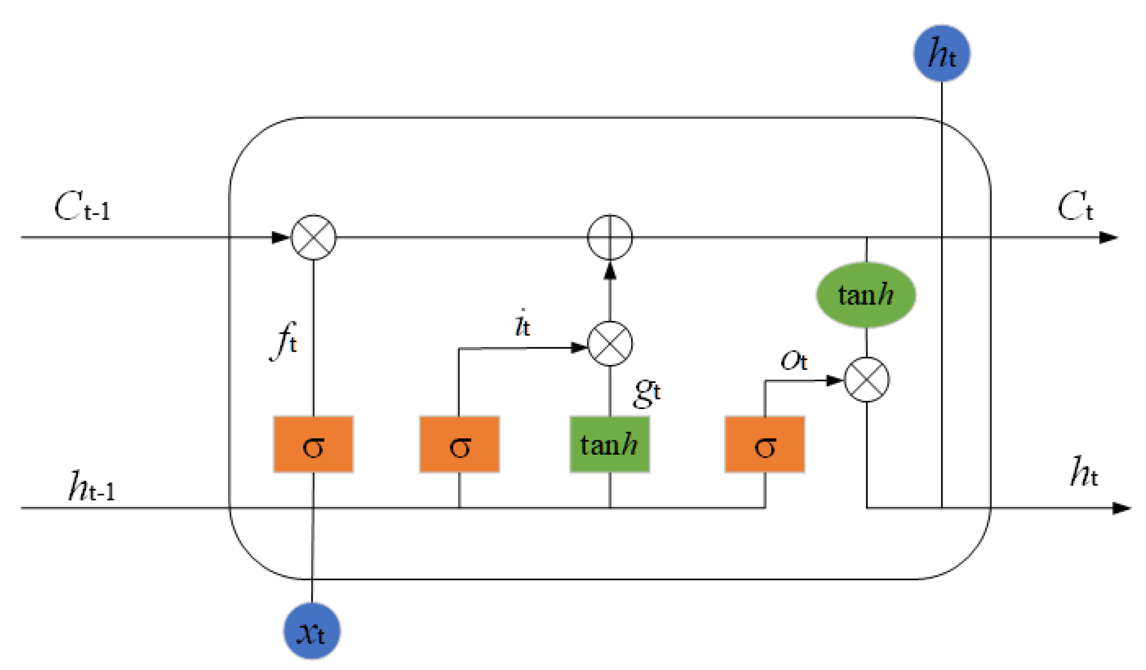
The Long Short-Term Memory (LSTM) network is a type of temporal recurrent neural network designed to address the challenges of vanishing and exploding gradients in standard Recurrent Neural Networks (RNNs). These issues can severely impact the predictive accuracy of models. To tackle these problems, the Long Short-Term Memory (LSTM) network was developed, aiming to overcome the limitations of RNNs in handling gradient-related issues [31]. The structure of an LSTM is illustrated in Figure 2.
Here, tanh represents the tanh function; σ is the sigmoid function; xt indicates the input at time t; Ct − 1 and Ct are the memory cells at time t − 1 and t, respectively; ht− 1 and ht represent the outputs at time t − 1 and t, respectively; gt is the long-term state value at time t; and ft,it and ot respectively control the outputs of the forget gate, input gate, and output gate.
The main forward propagation steps of the LSTM unit are as follows:
f t = σ ( W f [ h t 1 , x t ] + b f )
i t = σ ( W i [ h t 1 , x t ] + b i )
g t = tanh ( W c [ h t 1 , x t ] + b c )
Ct   =   ft Ct - 1   +   it gt
o t = σ ( W o [ h t 1 , x t ] + b o )
h t = o t · tanh ( C t )
Similarly to traditional RNNs, the RNN-LSTM network also employs the tanh activation function to prevent gradient vanishing. After extracting short-term data features, the underlying RNN performs temporally sequential training in the hidden layer. Through multiple iterations, the output at time step t is used as the input for time step t + 1. Subsequently, the output of the RNN is passed to the LSTM network. Based on the output of the underlying RNN, the LSTM learns long-term dependencies. The data undergoes filtering and updating processes in the forget gate and input gate, allowing the LSTM to selectively retain or discard long-term information, ultimately generating an output through the output gate.

2.3. Bayesian Optimization

Bayesian Optimization is a sequential model-based optimization method belonging to the class of derivative-free optimization techniques. It is widely used for black-box function optimization. This method constructs a surrogate model to approximate the black-box objective function and guides the iterative process using an acquisition function, aiming to find the global optimum with as few evaluations as possible [32]. Its core idea lies in continuously updating the posterior distribution by leveraging prior information and existing samples, thereby balancing exploration and exploitation to progressively approach the optimal solution. The Bayesian optimization algorithm primarily consists of two components: Gaussian process regression and an acquisition function.
(1)
Gaussian Process Regression
Gaussian Process Regression is a probability-based non-parametric regression method. Its core idea is to assume that the target function g to be predicted follows a Gaussian distribution, and then use existing data to estimate the mean and variance of this distribution. The predictive formula for Gaussian Process Regression is:
μ ( α ) = c * T ( C + σ n 2 I ) 1 b c o v ( α * ) = c c * T ( C + σ n 2 I ) 1 c *
where a* represents the input point corresponding to the predicted value of the target function; μ(a*) denotes the mean of the function at point a*; cov(a*) represents the covariance of the function at point a*; c is the covariance of the test point itself; c* is the covariance vector between the test point and the training data points; C is the covariance matrix among the training data points; σ n 2 is the variance of the Gaussian noise; I is the identity matrix; and b is the vector of target values for the training data points. This study employs the Matern5/2 kernel, whose mathematical formula is:
k ( x , x ) = σ f 2 1 + 5 r l + 5 r 2 3 l 2 exp 5 r l
In the equation: r = | x x ' | is the Euclidean distance, l is the length scale determining the smoothness of the function, and σ f 2 controls the output scale. The Matern 5/2 kernel is chosen because it imposes weaker smoothness assumptions compared to the RBF kernel, making it more suitable for scenarios where abrupt or irregular changes may occur in the hyperparameter space, such as performance jumps caused by learning rate variations. Additionally, the Matern kernel has been proven to achieve faster convergence and higher stability in practical machine learning optimization tasks.
(2)
Acquisition Function
This paper constructs the acquisition function based on Gaussian process regression. Gaussian process regression is used to predict the most probable current function values and compute the probability density function for each sampling point. Based on this probability density function, sampling is performed to obtain a new point as the input for the next optimization step. The formula for the acquisition function is:
a t + 1 = arg max a A E I ( a )
E I ( a ) = g min ( g ( a ) g min ) p ( g | D ) d g
where a represents a sampling point; at+ 1 denotes the next new sampling point; A represents the search space; EI(x) is the Expected Improvement function; gmin is the value of the current optimal solution; and p(g|D) represents the probability distribution of function g given the known data D.
(3)
Hyperparameter Estimation Method
The surrogate model itself also depends on several hyperparameters, such as the length scale l, the noise term σ n , and the output scale σ f . These hyperparameters are obtained by maximizing the marginal likelihood:
θ = arg max θ log p ( y X , θ )
The form of the marginal likelihood is:
log p ( y X , θ ) = 1 2 y T K 1 y 1 2 log | K | n 2 log 2
The optimization is typically performed by the L-BFGS-B algorithm. Maximizing the marginal likelihood automatically balances model fit and complexity, thereby preventing overfitting in the surrogate model and enhancing the stability of the overall Bayesian optimization process.
(4)
Numerical Robustness Guarantee
In Gaussian process modeling, the covariance matrix K may become near-singular due to numerical errors. To ensure stability, this study adopts the following treatments:
K K + σ n 2 I
where the noise term σ n 2 ensures that K remains strictly positive definite, facilitating matrix inversion. MATLAB (version 2023b)’s bayesopt framework automatically incorporates this noise term internally, thus maintaining strong numerical stability in our optimization process even in high-dimensional spaces.
(5)
Handling of Discrete and Integer Parameters
This study involves integer parameters, which bayesopt treats as ordered discrete variables. The kernel function distance calculation preserves their actual numerical values, ensuring the model’s predictive space remains continuously differentiable. Since all parameters in this study are either continuous or integer types, there is no need to employ specialized optimizers designed for mixed spaces.

2.4. Structure of the CNN-LSTM Short-Term Load Forecasting Model Based on Bayesian Optimization

To equip the model with the capability of automatic feature extraction, this study employs deep learning methods for its construction. Convolutional Neural Networks (CNNs), renowned for their powerful local feature extraction capabilities, typically utilize convolutional kernels to automatically learn effective features from data. However, due to the limited receptive field of convolutional kernels, CNNs struggle to capture long-term dependencies when processing time series data. To address this issue, this study introduces Long Short-Term Memory (LSTM) networks. Their gating mechanism can effectively capture contextual dependencies within time series. LSTMs selectively retain long-term historical information and forget irrelevant information through their carefully designed cell state and gating system (including the forget gate, input gate, and output gate). Furthermore, when dealing with multi-feature inputs, the original feature dimensionality is high. Direct processing is not only computationally inefficient but may also introduce noise, leading to decreased prediction accuracy.
To address the aforementioned challenges, this paper proposes a hybrid CNN-LSTM forecasting model that integrates feature engineering and Bayesian Optimization (BO). This method first performs feature selection through Pearson correlation analysis to reduce the input dimensionality. Subsequently, it utilizes CNN convolutional layers to extract local temporal features, followed by LSTM layers to capture long-term dependencies. Finally, the final predictions are generated through fully connected layers. Throughout the entire model construction process, the Bayesian optimization algorithm is employed to automatically search for the optimal hyperparameter combination, significantly enhancing model performance and learning efficiency. The workflow of the Bayesian optimization-based CNN-LSTM short-term load forecasting model is illustrated in Figure 3, with the specific steps as follows:
  • Feature Engineering Phase. First, historical data is preprocessed, including handling missing values, treating outliers, and normalization. Preliminary input features are selected. Then, Pearson correlation coefficient is used for correlation analysis to compute the correlation between each feature and the load value. Redundant features weakly correlated with the load are eliminated, forming a new feature set for subsequent model input.
  • Hyperparameter Optimization Phase. A Bayesian optimization framework is established, using the Root Mean Square Error (RMSE) of the prediction results as the objective function. The search space for hyperparameters is defined, including the number of CNN convolutional layers, the number and size of convolutional kernels, the number of LSTM layers, the number of LSTM units, dropout rate, learning rate, and batch size. The Gaussian process surrogate model and the Expected Improvement (EI) acquisition function are used to efficiently explore the parameter space and find the globally optimal hyperparameter combination.
This study treats the input sequence as a one-dimensional time-series signal, converting it into a pseudo-2D format before feeding it into the convolutional layer. The convolutional layer employs kernels of size 10 × 1, meaning each kernel covers 10 consecutive time steps along the temporal dimension. The design rationale is as follows:
  • Receptive field theory requires the convolutional kernel to cover the fundamental period or basic fluctuation window.
Based on data exploration results, the load sequence exhibits significant short-term fluctuations (within 5–15 steps). When the convolution kernel is set to 10, it precisely covers its typical local temporal structure, thereby being able to efficiently capture local trends and local change rates.
b.
The temporal receptive field of the convolutional layer can be described by the following formula:
R = ( k 1 ) d + 1
where k is the kernel length and d is the dilation factor.
c.
Effective coverage after combining convolutional and pooling layers:
The stride of the pooling layer is set to 10 times the length of the convolution kernel, which makes its function equivalent to compressing the convolutional features into a time window once. Thus, it achieves a 10-step-scale feature summary for the input sequence of length T and clearly distinguishes that the CNN captures “local short-term patterns” while the LSTM captures “global long-term dependencies”.
Therefore, the receptive field of the convolutional module aligns with the short-term fluctuation structure of the load data, representing a model design choice informed by data pattern analysis.
This study employs one convolutional layer with 32 kernels, based on the following considerations:
  • A single convolutional layer sufficiently covers the required local structure.
Since the data in this study does not exhibit complex multi-layer local nested patterns at short time scales, a single convolutional layer is adequate for local feature extraction, eliminating the need for stacking multiple layers.
b.
Avoiding parameter explosion and training instability caused by excessively deep convolutions.
Multiple convolutional layers would significantly increase the number of parameters, raising the risk of overfitting, particularly in power load forecasting tasks where sample sizes are limited. Preliminary experiments confirmed that a single convolutional layer achieves optimal performance.
c.
Rationale for evaluating dilated convolutions.
Dilated convolutions can expand the receptive field:
If a dilation factor d > 1 were used, the receptive field would expand significantly. However, the subsequent LSTM in this study already effectively models medium- to long-term dependencies. Moreover, dilated convolutions could disrupt local continuous features. Therefore, d = 1 was selected, and dilated convolutions were not employed.
While dilated convolutions represent a feasible alternative for pursuing a larger receptive field, the current CNN-LSTM combination already adequately covers features across all time scales, rendering additional modifications unnecessary.
3.
Predictive Model Construction Phase. The dataset is divided into training, validation, and test sets in chronological order. The model adopts a multi-layer encoder–decoder structure: the input layer receives the multi-dimensional time series data after feature selection; followed by 1–2 one-dimensional convolutional layers using the ReLU activation function to extract local features; a pooling layer to reduce feature dimensionality; a Dropout layer to prevent overfitting; then connected to 1–2 LSTM layers to capture long-term dependencies; and finally, the prediction results are output through a fully connected layer. Early stopping is used during training to prevent overfitting, and the Adam optimizer is used to update the network parameters.
4.
Prediction Phase. The trained CNN-LSTM model is used for load forecasting. The test set data is fed into the model, first passing through the CNN layers to extract deep local temporal features. The feature sequences are then fed into the LSTM layers to learn the long-term dependencies of the time series. Finally, the features are integrated through the fully connected layer to output the prediction results.
5.
Evaluation and Validation Phase. Multiple performance metrics are used to comprehensively evaluate the prediction results. This paper selects three metrics—Root Mean Square Error (RMSE), Mean Absolute Error (MAE), and Mean Absolute Percentage Error (MAPE)—to judge the accuracy of the predictions. Ablation experiments are conducted to verify the contribution of each module, including comparisons between a standalone LSTM model and the complete CNN-LSTM model, thereby validating the superiority and reliability of the proposed model.

3. Predictive Features and Evaluation Metrics

3.1. Data Preprocessing

Due to dimensional inhomogeneity between historical load data and relevant feature factors, directly inputting the raw data into the model for training would adversely affect prediction accuracy. Therefore, a normalization method is applied to process the data, with the calculation formula shown in Equation (16).
X = x x min x max x min
where X denotes the normalized input data; x represents the original input data; and xmax and xmin indicate the maximum and minimum values of x.

3.2. Load Feature Screening

In short-term power load forecasting, although high-dimensional features contain valuable information, some of them exhibit weak correlation with the target load. These redundant features not only prolong model training time but may also introduce noise, compromising prediction accuracy. To address this, this paper employs the Pearson correlation coefficient for feature screening [33]. By quantifying the linear correlation between each feature and the historical load, weakly correlated features are automatically filtered out, and only strongly correlated factors are retained as model inputs. This approach aims to enhance data quality, thereby accelerating model training speed while optimizing its predictive performance. The calculation formula is shown in Equation (17).
r x y = i = 1 n ( x i x ¯ ) ( y i y ¯ ) i = 1 n ( x i x ¯ ) 2 i = 1 n ( y i y ¯ ) 2
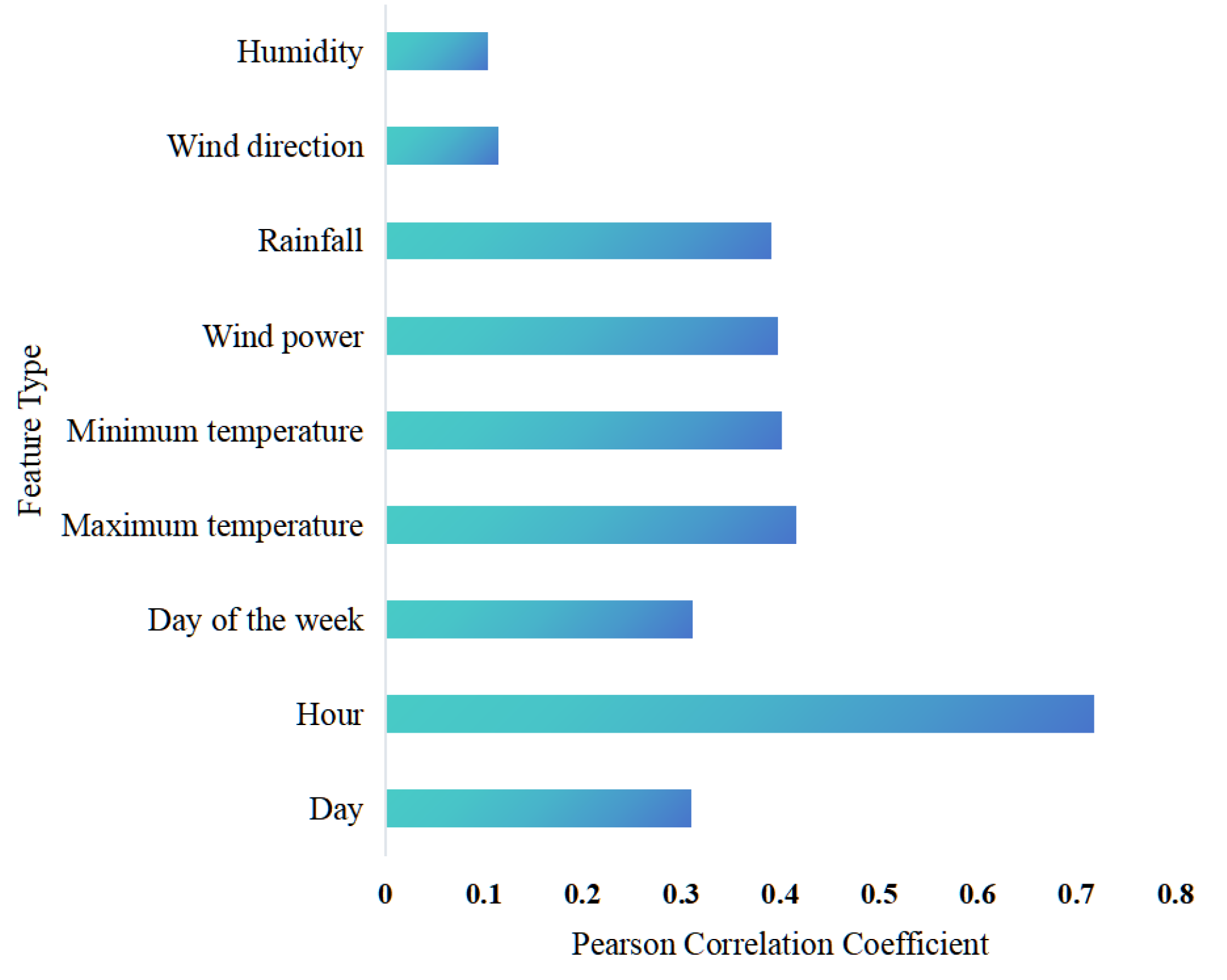
Here, x represents a specific feature such as temperature, and y represents the load value. By calculating rxy, the strength of the correlation between the feature and the load can be determined, thereby enabling effective feature screening. This method accurately measures the degree of linear correlation between variables x and y. In this study, load data from a typical industrial electrolytic aluminum process is used to calculate the Pearson correlation coefficient, thereby screening for load features with high correlation. The correlation coefficients between different factors and the output power are calculated, and the results are shown in Figure 4:
The calculation results indicate that wind direction and humidity exhibit relatively low correlation coefficients with output power. To simplify the model without compromising prediction accuracy, the following features are selected as training sample characteristics: day, hour, day of the week, maximum temperature, minimum temperature, wind power, and rainfall.

3.3. Parameter Settings

Based on the feature selection, this study employs the Bayesian optimization method to fine-tune the hyperparameters of the hybrid CNN-LSTM network model. The search range for the number of convolutional kernels in the CNN was set to (8, 16, 32, 64, 128, 256, 512), and the search range for the convolutional kernel size was set to (1, 2, 3). For the LSTM network, the search range for the number of hidden layer neurons was set to (10, 20, 30, 40, 50, 70, 100, 150), and the search range for the dropout rate was set to (0.1, 0.2, 0.3, 0.4, 0.5). The search range for the learning rate was set to (10−3, 10−2, 0.1, 0.2, 0.3, 0.5, 0.8, 1), and the search range for the batch size was set to (8, 16, 32, 64, 128, 256, 512). The Bayesian optimization algorithm was used to optimize the CNN-LSTM model.
To ensure training stability for both the convolutional and LSTM layers, this study implements the following mechanisms:
  • He Initializer
Used for initializing the input and recurrent weights of the convolutional and LSTM layers. This maintains healthy gradient flow when using the ELU activation function.
b.
L2 Regularization
Applied to suppress overfitting, with the optimal regularization strength automatically selected via Bayesian optimization.
c.
Dropout (rate = 0.25)
Applied to the output of the LSTM layer to reduce overfitting to specific local temporal windows.
d.
Gradient Clipping (Threshold = 1)
Prevents exploding gradients during LSTM training.
e.
Piecewise Learning Rate Schedule
The learning rate is halved every 200 epochs, ensuring more stable convergence in the later stages of training.
These measures collectively ensure that the network exhibits robust stability and strong generalization capability for the power load forecasting task.

4. Experiments

4.1. Experimental Setup

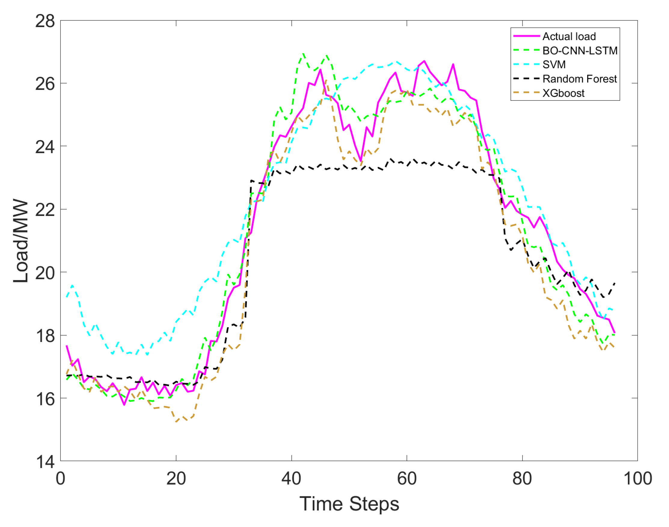
To validate the accuracy of the proposed model, typical industrial and agricultural load datasets from a location in Qinghai were utilized, including loads from electrolytic aluminum, agricultural irrigation, and alloy smelting. These three datasets contain electricity consumption data for the region from 1 January 2022 to 31 December 2022. Meteorological data include daily minimum temperature, maximum temperature, wind power, rainfall, etc. The load data is collected every 15 min, with the unit being MW, resulting in 96 collection points per day. The constructed input consists of load and meteorological data from the 14 days preceding the forecast day, and the output is the load data for the 96 sampling points on the forecast day. Data from 1 January 2022 to 16 December 2022, is used as the training set; data from 17 December 2022 to 30 December 2022, serves as the validation set; and data for 31 December 2022, is used for forecasting. The selection of a single day (December 31) as the test set is aimed at evaluating the model’s performance on a specific, representative day (year-end), providing a clear and focused comparison. The model’s generalization ability is further supported by its consistent performance across three different load types in subsequent sections. This study proposes a CNN-LSTM hybrid prediction model based on Bayesian optimization. Through ablation experiments, it is confirmed that Bayesian optimization is crucial for optimizing the model’s hyperparameters and improving prediction accuracy. Moreover, comparative experiments with random forests, support vector regression, and XGBoost show that the BO-CNN-LSTM model can achieve lower prediction errors and higher goodness-of-fit, demonstrating its superior performance.

4.2. Evaluation Metrics

To accurately evaluate the precision of the model proposed in this paper, the Root Mean Square Error (RMSE), Mean Absolute Error (MAE), and Mean Absolute Percentage Error (MAPE) were selected. These metrics are used to measure the discrepancy between the model’s predicted output and the actual load values, reflecting the accuracy and stability of the predictions. RMSE measures the overall magnitude of the prediction errors, MAE measures the average absolute prediction error, and MAPE calculates the percentage of relative error. Lower values for these metrics generally indicate a better fit of the predictive model to the actual load variations, providing strong quantitative evidence for assessing the performance of the load forecasting algorithm. The calculation formulas are as follows [34]:
E R M S E = 1 L i = 1 L ( y ˜ i y i ) 2
E M A E = 1 L i = 1 L | y ^ i y i |
E M A P E = 100 % L i = 1 L y ^ i y i y i
where y i is the actual load value; y ~ i is the predicted value from the model; and L is the total number of data samples.

4.3. Ablation Experiment Results Analysis

4.3.1. Load Forecasting for Industrial Electrolytic Aluminum (Ablation Study)

As can be seen from the data in Table 1, the Bayesian optimization-based CNN-LSTM model achieves higher accuracy than the other two methods; its MAE is reduced by 52.13 and 15.72 compared to the other two methods, respectively; its RMSE is reduced by 69.5 and 17.94 compared to the other two methods, respectively; and its MAPE is reduced by 2.97% and 0.95% compared to the other two methods, respectively. These quantitative comparisons have received further support from the prediction curves of the three models, as shown in Figure 5. These curves clearly indicate that the BO-CNN-LSTM model has superior fitting ability.

4.3.2. Load Forecasting for Agricultural Irrigation (Ablation Study)

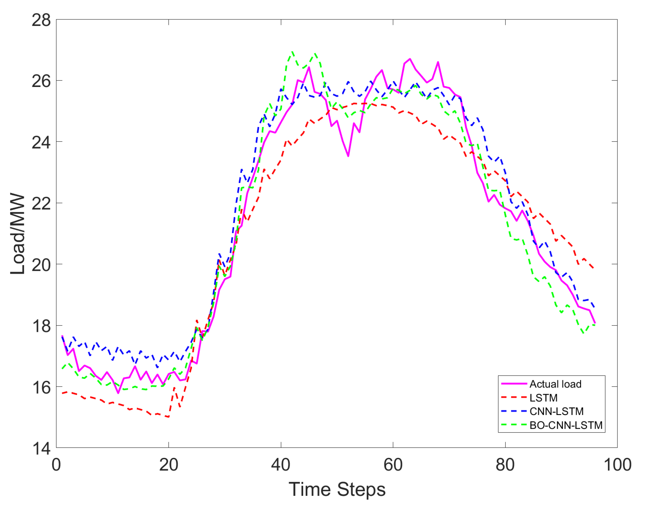
As can be seen from the data in Table 2, the Bayesian optimization-based CNN-LSTM model achieves higher accuracy than the other two methods; its MAE is reduced by 0.45 and 0.07 compared to the other two methods, respectively; its RMSE is reduced by 0.44 and 0.12 compared to the other two methods, respectively; and its MAPE is reduced by 2.25% and 0.48% compared to the other two methods, respectively. These quantitative comparisons have received further support from the prediction curves of the three models, as shown in Figure 6. These curves clearly indicate that the BO-CNN-LSTM model has superior fitting ability.

4.3.3. Load Forecasting for Industrial Alloy Smelting (Ablation Study)

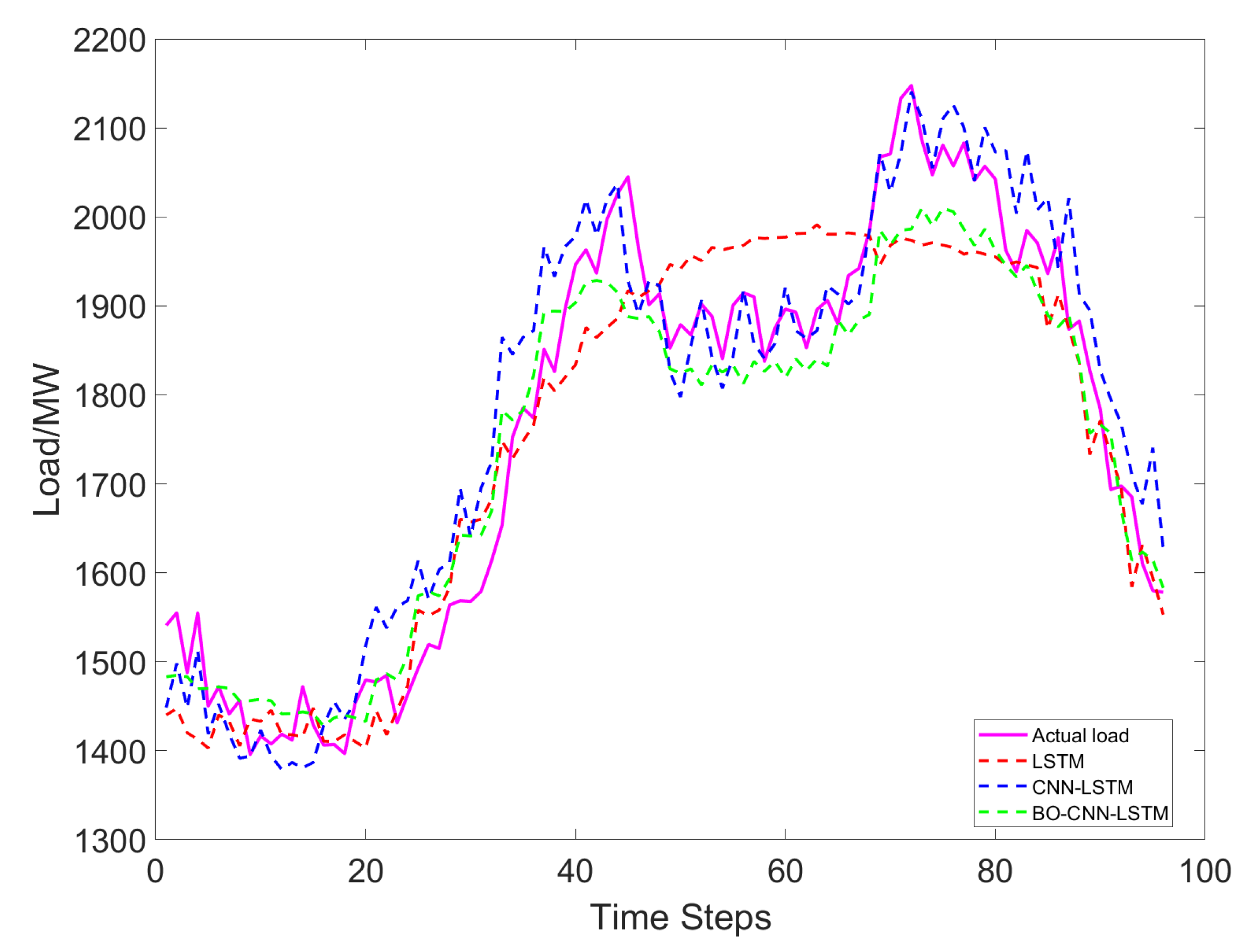
As can be seen from the data in Table 3, the Bayesian optimization-based CNN-LSTM model achieves higher accuracy than the other two methods; its MAE is reduced by 11.73 and 1.67 compared to the other two methods, respectively; its RMSE is reduced by 13.74 and 5.02 compared to the other two methods, respectively; and its MAPE is reduced by 0.63% and 0.26% compared to the other two methods, respectively. These quantitative comparisons have received further support from the prediction curves of the three models, as shown in Figure 7. These curves clearly indicate that the BO-CNN-LSTM model has superior fitting ability.
Based on the above prediction results, it can be concluded that the proposed Bayesian optimization-based CNN-LSTM model achieved the best performance in forecasting the three typical industrial and agricultural load types.

4.4. Comparison Results with Other Prediction Algorithms

4.4.1. Load Forecasting for Industrial Electrolytic Aluminum (Algorithm Comparison)

As can be seen from the data in Table 4, the Bayesian optimization-based CNN-LSTM model exhibited higher accuracy than the other three methods; its mean absolute error (MAE) was reduced by 48.55, 23.68, and 19.03 compared to the other three methods, respectively; its root mean square error (RMSE) was reduced by 54.27, 30.82, and 22.8 compared to the other three methods, respectively; and its mean absolute percentage error (MAPE) was reduced by 2.91%, 1.29%, and 1.06% compared to the other three methods, respectively. The intuitive comparison of the predicted curves in Figure 8 further confirms that the proposed BO-CNN-LSTM model outperforms these benchmark algorithms in terms of performance.

4.4.2. Load Forecasting for Agricultural Irrigation (Algorithm Comparison)

As can be seen from the data in Table 5, the Bayesian optimization-based CNN-LSTM model exhibited higher accuracy than the other three methods; its mean absolute error (MAE) was reduced by 0.48, 0.61, and 0.22 compared to the other three methods, respectively; its root mean square error (RMSE) was reduced by 0.59, 0.82, and 0.26 compared to the other three methods, respectively; and its mean absolute percentage error (MAPE) was reduced by 2.67%, 2.42%, and 1.08% compared to the other three methods, respectively. The intuitive comparison of the predicted curves in Figure 9 further confirms that the proposed BO-CNN-LSTM model outperforms these benchmark algorithms in terms of performance.

4.4.3. Load Forecasting for Industrial Alloy Smelting (Algorithm Comparison)

As can be seen from the data in Table 6: the Bayesian optimization-based CNN-LSTM model exhibited higher accuracy than the other three methods; its mean absolute error (MAE) was reduced by 27.42, 2.46, and 2.17 compared to the other three methods, respectively; its root mean square error (RMSE) was reduced by 30.27, 4.75, and 3.22 compared to the other three methods, respectively; and its mean absolute percentage error (MAPE) was reduced by 1.76%, 0.15%, and 0.13% compared to the other three methods, respectively. The intuitive comparison of the predicted curves in Figure 10 further confirms that the proposed BO-CNN-LSTM model outperforms these benchmark algorithms in terms of performance.
Based on the above prediction results, it can be concluded that the proposed CNN-LSTM model based on Bayesian optimization has the best prediction performance.

5. Conclusions

To address the challenges of short-term load forecasting in typical industrial and agricultural scenarios, this paper proposes a CNN-LSTM forecasting model based on Bayesian optimization. The effectiveness of this method was validated through theoretical explanation, case studies, systematic ablation experiments, and comparisons with various mainstream algorithms. The main conclusions are as follows:
  • Module contributions validated by ablation experiments: The ablation experiments conducted on three typical load datasets clearly demonstrate the role of each component. The results confirm the functional complementarity between CNN and LSTM, and underscore the critical importance of Bayesian optimization for automated hyperparameter tuning in maximizing the hybrid model’s predictive performance.
  • Superior performance demonstrated through comparative analysis: Comparative experiments with SVR, Random Forest, and XGBoost demonstrate the proposed model’s superior accuracy and robustness across different load types, proving its enhanced capability in capturing complex spatiotemporal dependencies.
  • Feature engineering and automated optimization are key enablers: The feature selection and Bayesian optimization strategy effectively enhanced data quality and model performance, improving the method’s practicality and reproducibility.
In summary, the proposed model demonstrates high application potential for power system dispatch. Despite these strengths, this study has limitations, such as the computational demands of the model and its reliance on high-quality, comprehensive data. Future work will focus on developing more lightweight architectures, incorporating diverse data sources to improve generalization, and exploring probabilistic forecasting frameworks and explainable AI techniques to enhance robustness and interpretability in real-world applications.

Author Contributions

Conceptualization, P.D., H.J. and A.H.; methodology, J.S.; data curation, Z.D.; writing—original draft preparation, P.D. and X.C.; writing—review and editing, L.C. and X.C.; visualization, H.J. and L.C. All authors have read and agreed to the published version of the manuscript.

Funding

This research was funded by the Science and Technology Project of State Grid Qinghai Electric Power Company. The name of the funded project is Research on Identification of Typical Demand Side Resources Characteristics and Analytical Method for Adjustable Potential, funder: State Grid Qinghai Electric Power Company, funding number: SGYXFW00KHJS2500057.

Data Availability Statement

The original contributions presented in this study are included in the article. Further inquiries can be directed to the corresponding author.

Conflicts of Interest

Authors Pengyang Duan, Huannian Jiao, Zheng Dai and Liang Cheng were employed by Marketing Service Center, State Grid Qinghai Electric Power Company. Author Jianying Sun was employed by State Grid Qinghai Electric Power Company. The authors state that during the course of this research, there were no any commercial or financial relationships that could be construed as potential conflicts of interest. The author declares that this research was funded by the Science and Technology Project of State Grid Qinghai Electric Power Company. The specific participation of the funding party in this research is as follows: they provided experimental data and defined the industrial application scenarios.

References

  1. Kang, C.Q.; Chen, Q.X.; Xia, Q. Prospects of low carbon electricity. Power Syst. Technol. 2009, 33, 1–7. [Google Scholar]
  2. Zhao, X.; Sun, C.; Zhong, Z.; Liu, S.; Yang, Z. Effect of market structure on renewable energy development—A simulation study of a regional electricity market in china. Renew. Energy 2023, 215, 118911. [Google Scholar] [CrossRef]
  3. Zhou, J.; Huang, A.P.; Xiao, J.R.; Cheng, T.; Liang, C. Analysis of power load forecasting technology based on deep neural networks. Electr. Technol. Econ. 2024, 145–148. [Google Scholar]
  4. Niu, D.X.; Cao, S.H.; Lu, J.C. Power Load Forecasting Technology and Its Applications; China Electric Power Press: Beijing, China, 2009. [Google Scholar]
  5. Li, D.; Sun, G.F.; Miao, S.W. Short term power load forecasting method based on multi dimensional time series information fusion. Proc. CSEE 2023, 43, 94–106. [Google Scholar]
  6. Sun, H.; Wan, C.; Cao, Z.J.; Li, Y.Y.; Ju, P. Short term probabilistic load forecasting based on conditional GAN curve generation. Autom. Electr. Power Syst. 2023, 47, 189–199. [Google Scholar]
  7. Jiang, M.Y.; Xu, L.; Zhang, K.J.; Ma, Y. Wind speed time series forecasting via seasonal index adjusted recurrent neural networks. Acta Energiae Solaris Sin. 2022, 43, 444–450. [Google Scholar]
  8. Jiang, D.L.; Li, T.H.; Liu, W.H. Short term power load forecasting using a similar day SAE DBiLSTM model. J. Electr. Eng. 2022, 17, 240–249. [Google Scholar]
  9. Chodakowska, E.; Nazarko, J.; Nazarko, Ł. Arima models in electrical load forecasting and their robustness to noise. Energies 2021, 14, 7952. [Google Scholar] [CrossRef]
  10. Wu, L.Z.; Kong, C.; Chen, W. Short-term load forecasting based on linear regression under MapReduce framework. J. Lanzhou Univ. Technol. 2021, 47, 97–104. [Google Scholar]
  11. Nijhawan, P.; Bhalla, V.K.; Singla, M.K.; Gupta, J. Electrical Load Forecasting using SVM Algorithm. Int. J. Recent Technol. Eng. 2020, 8, 4811–4816. [Google Scholar] [CrossRef]
  12. Feng, Y.; Song, Y.B.; Jin, S.; Feng, J.; Shi, X.; Yu, Y.; Huang, X. An improved deep learning short-term load forecasting model based on random forest algorithm and rough set theory. Power Gener. Technol. 2023, 44, 889–895. [Google Scholar]
  13. Zheng, H.; Yuan, J.; Chen, L. Short-term load forecasting using EMD-LSTM neural networks with a Xgboost algorithm for feature importance evaluation. Energies 2017, 10, 1168. [Google Scholar] [CrossRef]
  14. Wei, D.; Yang, J.T.; Han, S.R.; Zhu, Z. Construction of building load forecasting model based on XGBoost-neural network. Sci. Technol. Eng. 2023, 23, 12604–12611. [Google Scholar]
  15. Ye, Y.S.; Zhang, J. SVM based short term power load forecasting with time series. Mod. Inf. Technol. 2020, 4, 17–19. [Google Scholar]
  16. An, Y.K.; Zhu, Y.D. Power load forecasting via linear regression and exponential smoothing. Power Equip. Manag. 2021, 177–179. [Google Scholar]
  17. Sui, S.W.; Yu, H.M.; Jian, Z.M.; Zhao, Y. Large power load forecasting and billing based on an improved adaptive Kalman filter. Comput. Meas. Control 2023, 31, 149–155. [Google Scholar]
  18. Shi, L.J. Transformer Fault Diagnosis Based on Grey Wolf Optimizer Tuned Support Vector Machine. Master’s Thesis, North China University of Water Resources and Electric Power, Zhengzhou, China, 2021. [Google Scholar]
  19. Zhu, B.; Zhou, X.C. Load forecasting and optimal dispatch of power systems using artificial neural networks. Autom. Appl. 2024, 65, 89–91. [Google Scholar]
  20. Zhao, J.; Cheng, P.; Hou, J.; Fan, T.; Han, L. Short term load forecasting of multi scale recurrent neural networks based on residual structure. Concurr. Comput. Pract. Exp. 2023, 35, e7551. [Google Scholar] [CrossRef]
  21. Zhao, B.; Wang, Z.P.; Ji, W.J.; Gao, X.; Li, X. Short term power load forecasting method based on attention mechanism of CNN-GRU. Power Syst. Technol. 2019, 43, 4370–4376. [Google Scholar]
  22. Chen, L.; Wang, Z.; Wang, G. Application of LSTM network under deep learning framework in short term power load forecasting. Electr. Power Inf. Commun. Technol. 2017, 15, 8–11. [Google Scholar]
  23. Zhou, M.; Gao, T.; Li, C.G.; Jiang, C.L. Short term power load forecasting using GRU neural network. Sci. Technol. Innov. Appl. 2018, 52–53+57. [Google Scholar]
  24. Xu, Y.; Xiang, Y.F.; Ma, T.X. Short term power load forecasting based on EMD CNN LSTM hybrid model. J. North China Electr. Power Univ. (Nat. Sci. Ed.) 2022, 49, 81–89. [Google Scholar]
  25. Sun, L.L.; Fang, H.B.; Zhu, X.X.; Hu, L.; Qi, L. Stock prediction based on XGBoost model optimized by grid search. J. Fuyang Norm. Univ. (Nat. Sci. Ed.) 2021, 38, 97–101. [Google Scholar]
  26. Long, Q.Q.; Tang, X.Y. Prediction model based on R language algorithm and random search—Taking heart failure death risk prediction as an example. Mod. Inf. Technol. 2024, 8, 91–93+98. [Google Scholar]
  27. Liu, Z.L.; Ju, X.; Zhang, Y.F.; Huang, Y.C. Random-forest hyper parameter optimization via improved random search algorithm. Netw. Secur. Technol. Appl. 2022, 49–51. [Google Scholar]
  28. Li, Y.B.; Wei, T.T.; Jia, H.; Li, S. Photovoltaic power generation forecasting based on genetic algorithm. J. Zhongyuan Univ. Technol. 2024, 35, 1–5. [Google Scholar]
  29. Feng, Q.; Li, Q.; Quan, W.; Pei, X.M. Overview of multi objective particle swarm optimization algorithms. Chin. J. Eng. 2021, 43, 745–753. [Google Scholar]
  30. Zhao, Y.R.; Wang, Y.C.; Yuan, L.Z. Short term power load forecasting based on SSA-CNN-LSTM. Mod. Ind. Econ. Inf. 2024, 14, 169–170. [Google Scholar]
  31. Wang, R.Z. Research on 10kV Distribution Network Single Phase Grounding Fault Line Selection. Master’s Thesis, China University of Mining and Technology, Xuzhou, China, 2022. [Google Scholar]
  32. Wang, G.; Jia, R.; Liu, J.; Zhang, H. A hybrid wind power forecasting approach based on Bayesian model averaging and ensemble learning. Renew. Energy 2020, 145, 2426–2434. [Google Scholar] [CrossRef]
  33. Ji, D.Y.; Jin, F.; Dong, L.; Zhang, S.; Yu, K.Y. Photovoltaic power station data reconstruction based on Pearson correlation coefficient. Proc. CSEE 2022, 42, 1514–1523. [Google Scholar]
  34. Zhou, Y.; Wang, J.; Liu, Y.; Yan, R.; Ma, Y. Incorporating deep learning of load predictions to enhance the optimal active energy management of combined cooling, heating and power system. Energy 2021, 233, 121134. [Google Scholar] [CrossRef]
Figure 1. Convolutional Neural Network Architecture Diagram.
Energies 18 06217 g001
Figure 2. LSTM Structure.
Energies 18 06217 g002
Figure 3. Workflow of Bayesian Optimization-based CNN-LSTM Short-Term Load Forecasting.
Energies 18 06217 g003
Figure 4. Analysis Results of Pearson Correlation Coefficients.
Energies 18 06217 g004
Figure 5. Prediction Results of Different Models for Industrial Aluminum Electrolysis (Ablation Study).
Energies 18 06217 g005
Figure 6. Prediction Results of Different Models for Agricultural Irrigation (Ablation Study).
Energies 18 06217 g006
Figure 7. Prediction Results of Different Models for Industrial Alloy Smelting (Ablation Study).
Energies 18 06217 g007
Figure 8. Prediction Results of Different Models for Industrial Aluminum Electrolysis (Algorithm Comparison).
Energies 18 06217 g008
Figure 9. Prediction Results of Different Models for Agricultural Irrigation (Algorithm Comparison).
Energies 18 06217 g009
Figure 10. Prediction Results of Different Models for Industrial Alloy Smelting (Algorithm Comparison).
Energies 18 06217 g010
Table 1. Model Evaluation Metrics for Ablation Study (Industrial Electrolytic Aluminum).
ModelRMSEMAEMAPE (%)
LSTM107.8882.594.66
CNN-LSTM56.3246.182.64
BO-CNN-LSTM38.3830.461.69
Table 2. Model Evaluation Metrics for Ablation Study (Agricultural Irrigation).
ModelRMSEMAEMAPE (%)
LSTM1.121.024.88
CNN-LSTM0.80.643.11
BO-CNN-LSTM0.680.572.63
Table 3. Model Evaluation Metrics for Ablation Study (Industrial Alloy Smelting).
ModelRMSEMAEMAPE (%)
LSTM75.4162.823.47
CNN-LSTM66.6952.763.10
BO-CNN-LSTM61.6751.092.84
Table 4. Model Evaluation Metrics for Algorithm Comparison (Industrial Electrolytic Aluminum).
ModelRMSEMAEMAPE (%)
SVM92.6579.014.6
Random Forest69.254.142.98
XGBoost61.1849.492.75
BO-CNN-LSTM38.3830.461.69
Table 5. Model Evaluation Metrics for Algorithm Comparison (Agricultural Irrigation).
ModelRMSEMAEMAPE (%)
SVM1.271.045.39
Random Forest1.51.175.05
XGBoost0.940.783.71
BO-CNN-LSTM0.680.562.63
Table 6. Model Evaluation Metrics for Algorithm Comparison (Industrial Alloy Smelting).
ModelRMSEMAEMAPE (%)
SVM91.9478.514.6
Random Forest66.4253.552.99
XGBoost64.8953.262.97
BO-CNN-LSTM61.6751.092.84
Disclaimer/Publisher’s Note: The statements, opinions and data contained in all publications are solely those of the individual author(s) and contributor(s) and not of MDPI and/or the editor(s). MDPI and/or the editor(s) disclaim responsibility for any injury to people or property resulting from any ideas, methods, instructions or products referred to in the content.