Distribution-Level PV Representative Bands: Blockwise BGMM and NSGA-II for Coverage and Tail-Risk

Abstract

Power system planning requires reliable information about feeder-level photovoltaic (PV) variability, but point forecasts are often uncertain. This study proposes a procedure for constructing explainable, frequency-aware representative bands for daily PV output at the feeder section level. The method segments the annual PV series into homogeneous periods, derives reference shapes from probabilistically clustered daily profiles, and selects an upper band that balances coverage, shape fidelity, and upper tail risk through multi-objective optimization. Validation on real feeder data shows that the bands enclose frequent and recent shapes (average weighted coverage ≈ 0.85), limit upward exceedances (≈0.06), and remain compact. The approach supports practical threshold and reserve planning and provides a transparent complement to point forecasts by emphasizing typical operating regimes while remaining cautious about extremes.

1. Introduction

The rapid growth of solar photovoltaic capacity has increased variability and intermittency in modern power systems. As of 2024, variable renewables account for about 67.5% of renewable capacity, heightening concerns about maintaining reliable supply and secure operation under changing weather and demand conditions [1]. As a result, forecasting has become a central tool for power system planning and real-time operation, with a growing body of statistical and machine learning approaches emerging. However, photovoltaic output remains strongly weather-dependent. This leads to persistent forecast errors and ongoing uncertainty across different time horizons and locations. Numerous studies have pointed out that such uncertainty cannot be fully addressed through point forecasts alone. Therefore, relying solely on point forecasts presents limitations, making it challenging to apply them directly in operational settings [2].

To address these limitations, recent research has focused on using representative patterns rather than relying solely on forecasts [3,4,5,6,7]. Representative patterns summarize the key variability characteristics of solar PV output, providing typical output scenarios that can be used in system analysis and planning without the need to consider the entire time series [8]. For example, analyzing multi-year solar output data to extract typical days and extreme conditions can represent the overall distribution with only a few periods [9]. This approach reduces computational complexity while capturing key intermittency patterns, thus helping to compensate for or replace the uncertainty caused by forecast errors.

Various techniques have been explored in the literature to generate representative patterns. Clustering methods are commonly used, grouping large datasets of daily or hourly output into clusters of similar patterns, from which representative days are selected [10]. For instance, Tanoto et al. [11] applied k-means clustering and algorithmic grouping to categorize historical solar output patterns into several representative types, while Liu et al. [12] used hierarchical clustering to derive representative operational periods for power planning models. Some studies have also formalized the selection of representative days as an optimization problem. Yeganefar et al. [8] proposed the Carpe Diem method using mixed-integer programming to select representative days for long-term planning, and Barbar et al. [10] examined methods for selecting representative days that account for intermittent renewable energy impacts. Optimization-based approaches focus directly on minimizing errors related to planning objectives, distinguishing them from clustering methods. Statistical or scenario-based methods also exist, such as generating multiple random scenarios and selecting the most representative few based on probability distributions [13]. For example, Li et al. [14] combined k-means clustering with discrete Markov chains to create a Typical Solar Radiation Year by considering seasonal occurrence probabilities. Tejada-Arango et al. [15] proposed an enhanced method that optimizes both representative days and system states, considering energy storage, while Sun et al. [16] developed a cost-oriented method for selecting representative days based on investment decision impacts. Additionally, various methods to reduce the time scale have been proposed, and recent comprehensive reviews summarize the trends and limitations of such time reduction techniques [17].

Overall, these studies demonstrate that representative-pattern approaches can substantially reduce the dimensionality of multi-year time series while preserving the main variability features needed for planning and operation. Optimization-based frameworks typically achieve favorable trade-offs between multiple criteria such as coverage, diversity, and cost-related performance, but they can be computationally demanding and often require case-specific tuning to a particular horizon or region. Clustering- and scenario-based methods are widely used in practice due to their conceptual simplicity and flexibility, yet they may provide less explicit control over how rare extremes and recent conditions are weighted, especially when the focus shifts from system-wide averages to individual feeder sections. Thus, rather than identifying a single best family of methods, the existing literature suggests that the most appropriate approach depends on the planning objective, the spatial and temporal granularity, and the required level of interpretability.

Despite the advances in representative pattern generation, there are several areas for further exploration in the existing literature. First, most studies focus on aggregated output at the national or regional level, which fails to fully account for spatial distribution or specific characteristics of individual feeder sections in the distribution network. Solar PV output at smaller distribution line sections can vary due to geographical location and load characteristics, but most representative pattern generation has concentrated on wide-area average patterns. Second, extreme conditions are often underrepresented. Representative day selection typically prioritizes average or typical days, leading to the exclusion of extreme conditions such as cloudy or clear days. Excluding such extreme days can result in underestimating storage capacity or backup needs, and some studies have reported that omitting extreme load days significantly underestimates investment costs and required capacity [3]. Third, the consideration of probabilistic reliability is insufficient. Current representative patterns are typically presented as deterministic profiles, with no explicit indication of the probability or uncertainty range associated with each pattern. While some recent studies, including those by Fitiwi et al. [18] and Yin et al. [19], have explored risk-averse probabilistic scenarios, a comprehensive approach that addresses the entire probability distribution remains largely unexplored. For feeder- and feeder-section-level applications, this gap makes it difficult to relate representative patterns to explicit reliability levels, motivating the use of a probabilistic representative pattern generation framework in this study.

This paper aims to address these limitations by proposing a probabilistic representative pattern generation method and applying it to a more granular distribution line unit level. The proposed method analyzes the probability distribution of solar output at each feeder section, generating representative output patterns that reflect reliability levels. A probabilistic formulation is chosen so that the resulting bands can be interpreted directly in terms of empirical coverage and exceedance probabilities at the feeder section level, rather than as purely deterministic typical days. This approach enhances spatial granularity and the inclusion of extreme conditions, which have been overlooked in previous methods. By providing probabilistic interpretations for the representative pattern set, the method is intended to improve the practical application of distribution network operation and planning.

The structure of this paper is as follows. In Section 2, the theoretical background and detailed procedure for the proposed representative pattern generation technique are described. Section 3 presents the application of the proposed method to real distribution line data, followed by analysis and interpretation of the results. Finally, Section 4 summarizes the main findings of the study and offers suggestions for future research directions.

2. Proposed Method for Representative Pattern Generation

This paper proposes a method that summarizes daily photovoltaic (PV) behavior at the distribution line section level from a probabilistic and frequency-aware perspective. The core idea is to first partition the time span into blocks where statistical properties are relatively stable, then structure daily curves within each block using a probabilistic model, and finally select an upper quantile curve and band width using multi-objective optimization that balances coverage, shape fidelity, upper tail risk, interval quality, and frequency consistency. This design reduces non-stationarity induced by seasonality and asset changes, and it targets both consistency and conservativeness that are meaningful for system analysis.

It is noted that the individual components of the framework, such as the LSTM autoencoder, BGMM, and NSGA-II, are standard methods. The novelty of this study is in how these elements are combined and tailored to the distribution-level PV banding problem, yielding a transparent procedure that links representative bands to feeder section coverage and upper tail risk.

2.1. Data Preprocessing and Daily Profile Construction

In operating and planning renewable resources, raw PV time series often contain irregular sampling intervals, missing observations, and outage periods. Using such data without normalization distorts pattern recognition, introduces statistical bias, and can lead to misleading representative curves. The raw measurements are therefore converted into a consistent 24-h day-level structure to secure reliability and reproducibility of the downstream analysis [20]. The goal of this study is to produce representative patterns (upper curve and bands) in a reliable manner, which requires removing days with virtually no generation. If inactive days remain, the frequent zeros bias quantiles downward and dilute the features of peak and variable periods that matter operationally. To avoid this structurally, the power trace is resampled, and the energy is aggregated so that each day becomes a 24-dimensional vector on a common scale, after which activity is classified based on the daily total energy.

Specifically, if the measured quantity is power $P_d\left(t\right)$, $E_{d,h}$, the hourly energy for day $d$ and hour $h$, is computed as shown in Equation (1),

$$E_{d,h}=\sum _{t\in [h,h+1]}{P}_d\left(t\right)∆t$$

(1)

where $E_{d,h}$ denotes the energy of time $h$ on day $d$. The daily total energy is then defined as shown in Equation (2),

$$E_{d,tot}=\sum _{t=0}^{23}{E}_{d,h}$$

(2)

where $E_{d,tot}$ is the total PV energy of day $d$. Using $E_{d,tot}$ active days with a minimum effective threshold $\epsilon$ is identified as shown in Equation (3),

$$d=\left\{\begin{array}{cc}active\left(d\right)& E_{d,tot}\ge \epsilon \\ deactive\left(d\right)& E_{d,tot}<\epsilon \end{array}\right.$$

(3)

This process is not a mere shape-matching resampling to 24 points. It preserves the meaning of the time axis through energy aggregation and systematically removes operationally negligible days. As a result, all active days are represented as homogeneous 24-dimensional energy vectors, which provide a robust input for the subsequent change-point-based block segmentation, Bayesian Gaussian mixture model (BGMM) probabilistic clustering, and Non-dominated Sorting Genetic Algorithm II (NSGA-II) optimization of the representative upper curve and band without interference from inactive day noise. This preprocessing is a prerequisite for the reliability of representative pattern estimation and supplies a sturdy input even when frequency–recency weights and spike-sensitive indicators are applied later.

2.2. Blockwise Segmentation and Micro-Splitting

Even within a single distribution-feeder section, the generation regime changes over time. Seasonal and irradiance cycles, asset additions or replacements, planned outages, faults or curtailment, soiling and aging, and changes in control policy alter both the daily total energy and the statistics of the 24-h profile. Estimating representative patterns under a single-distribution assumption over the full span can blur such regime shifts and may yield curves that are unsafe for conservative planning and operation. To prevent this, the record is partitioned into quasi-stationary blocks and representatives are estimated for each block.

Segmentation uses only endogenous statistics of the PV series without exogenous weather variables. First, the daily 24 h profiles are embedded with an LSTM autoencoder as shown in Equation (4),

$$z_t=Enc\left(x_t\right)$$

(4)

where $z_t$ is a latent vector that summarizes the shape of the power series $x_t$ at time $t$. In the segmentation step, the LSTM autoencoder is trained to reconstruct 24 h normalized PV profiles. The encoder consists of a single LSTM layer with 64 hidden units followed by a 16-dimensional latent vector, and the decoder mirrors this structure to reconstruct the input sequence. The model is trained with mean squared error on one year of daily profiles using early stopping. This architecture is standard and is used only to obtain a compact latent representation for shape change detection; it does not perform multi-step forecasting. Let the left and right local latent means around a candidate boundary $t$ be ${\overline{z}}_L\left(t\right)$ and ${\overline{z}}_R\left(t\right)$ with window size $\omega$. They are defined as shown in Equation (5),

$${\overline{z}}_L\left(t\right)={\displaystyle \frac{1}{\omega }}\sum _{i=t-\omega +1}^t{z}_i, {\overline{z}}_R\left(t\right)={\displaystyle \frac{1}{\omega }}\sum _{i=t+1}^{t+\omega }{z}_i$$

(5)

where $\omega$ is the window length.

Using these quantities, a shape-change indicator is computed as shown in Equation (6),

$$D\left(t\right)=1-{\displaystyle \frac{{\overline{z}}_L\left(t\right)·{\overline{z}}_R\left(t\right)}{\left|{\overline{z}}_L\left(t\right)\right|\left|{\overline{z}}_R\left(t\right)\right|}}$$

(6)

Shape consistency is also quantified with dynamic time warping as a standard elastic metric for time-aligned profile comparison, and latent-space change points are monitored for distribution-level PV regimes where abrupt shifts may occur [21,22]. For each candidate split day $t$, two signals are combined: a latent change score and a Dynamic Time Warping (DTW)-based shape consistency score. The latent change score measures the difference between the average latent vectors in a left window and a right window around day $t$, and therefore reacts to regime shifts in the compressed representation. In parallel, a DTW distance between the average daily profiles on each side is computed to quantify whether the typical shapes before and after $t$ remain similar. A split is accepted only when latent change score exceeds a fixed threshold and the DTW distance indicates a clear discontinuity in shape; if the latent change is small or the DTW distance remains low, the candidate is discarded.

A standardized score is then formed as shown in Equation (7),

$$Z\left(t\right)={\displaystyle \frac{D\left(t\right)-{\mu }_D}{{\sigma }_D}}$$

(7)

where $Z\left(t\right)$ is the shape-change score, and ${\mu }_D$ and ${\sigma }_D$ are the mean and standard deviation of $D\left(t\right)$. Candidate boundaries are times where $Z\left(t\right)\ge k$ and $D\left(t\right)$ is locally maximal. The threshold $k$ is not chosen ad hoc. It is selected from a small grid based on segment-membership stability and the robustness of downstream metrics under ±10–20 percent perturbations. In our setting $k=2$ was the most stable and is adopted here.

In addition to the main split candidates, micro-splits are allowed to isolate rare spike-like days. Let $m_t$ be the daily maximum normalized PV value and let $q_{0.98}$ denote the 98th percentile of $m_t$ within a provisional block. A combined micro-split score is defined as shown in Equation (8),

$$s_t=\alpha \overline{D}\left(t\right)+\left(1-\alpha \right)1\left\{m_t\ge q_{0.98}\right\}$$

(8)

where $\overline{D}\left(t\right)$ is the latent change score normalized to [0, 1] within the block, 1{$·$} equals 1 if the condition holds and 0 otherwise, and $\alpha \in \left(\mathrm{0,1}\right)$ is a fixed weight. A micro-split is triggered when $s_t$ exceeds a fixed high threshold (chosen once for all sections), so that micro-splits are reserved for days that are both shape-atypical in the latent space and exceptionally high in terms of daily maximum. This rule formally defines the combined score mentioned above and ensures that micro-splits are restricted to genuinely unusual spike days.

To avoid mixing spike-heavy periods, an additional refinement step is applied that detects runs of days whose daily maximum exceeds the block-level percentile for at least three consecutive days (metric = daymax). At most one additional cut is inserted per block around the center of such a run. Although some boundaries may align with seasonal transitions or asset events, the procedure is fully endogenous and requires no external labels. Active days are selected by an energy threshold $\epsilon ={10}^{-6}$ with a minimum of 14 active days. The LSTM auto-encoder is trained for 60 epochs (hidden = 64, latent $d_z=16$, Adam ${10}^{-3}$). The shape-change indicator uses left/right latent means with window $\omega =14$ days; peaks above $\mu +1.5\sigma$ with a minimum gap of 14 days define candidates, capped at two splits per section. These choices ensure reproducibility while keeping the procedure lightweight. The latent dimension is fixed at 16 and the window size at ω = 14 days, which is long enough to smooth day-to-day noise but short enough to respond to regime shifts over a few weeks. The 14-day minimum gap avoids spurious back-to-back splits while still allowing multiple blocks when sustained shifts occur.

Within each block, daily curves are clustered probabilistically so that frequency, recency, and uncertainty are reflected. On that basis, conservative yet frequency-consistent upper representative curves and confidence bands are derived. This directly supports conservative planning and operation at the feeder section level, where rare high outputs and operational constraints must be considered together. Algorithm 1 summarizes the shape-based segmentation with micro-splits used to define these blocks.

Algorithm 1 Shape-based Segmentation with Micro-splits

Input: Daily 24 h normalized PV profiles ${\left\{y_t\right\}}_{t=1}^T$ Hyperparameters: - Latent dimension (16), LSTM hidden units (64) - Shape-change window size $w=14$ days and minimum gap between splits - Threshold $k$ for the standardized shape-change score $Z\left(t\right)$ - Percentile level for spike detection (98th percentile of daily maxima) - Micro-split weight $\alpha$ and fixed high threshold for $s_t$ Output: Set of segmentation boundaries (main splits and micro-splits) Train LSTM autoencoder Train an LSTM autoencoder on $y_t$ to reconstruct daily profiles using mean squared error and early stopping, and obtain latent vectors for each day $t$ Compute latent change scores For each candidate day $t$ with $\omega$ days on both sides:   (a) Compute mean latent vectors ${\overline{z}}_L\left(t\right)$ and ${\overline{z}}_R\left(t\right)$ over the $\omega$ days before and after $t$   (b) Compute a raw latent change score $D\left(t\right)=1 - {\displaystyle \frac{{\overline{z}}_L\left(t\right)·{\overline{z}}_R\left(t\right)}{\left|{\overline{z}}_L\left(t\right)\right|\left|{\overline{z}}_R\left(t\right)\right|}}$ Standardize $D\left(t\right)$ over all $t$ to obtain the shape-change score $Z\left(t\right)$ Select main split candidates Identify candidate boundaries where $Z\left(t\right)\ge k$ and $D\left(t\right)$ is locally maximal, enforcing a minimum temporal gap between neighboring candidates Apply DTW-based shape consistency check For each candidate boundary $t$   (a) Compute representative daily profiles on the left and right of $t$   (b) Compute the DTW distance between the two representative profiles Retain $t$ as a main split only if the latent change score exceeds its threshold and the DTW distance indicates a clear discontinuity in shape Add micro-splits for spike days Within each provisional block defined by the main splits:   (a) Compute the daily maximum $m_t$ and the 98th percentile $q_{0.98}$ of $m_t$ in the block   (b) Normalize the latent change scores within the block to obtain $\overline{D}\left(t\right)\in \left[\mathrm{0,1}\right]$   (c) For each day $t$, compute the combined micro-split score     $s_t=\alpha \overline{D}\left(t\right)+\left(1 - \alpha \right)1\left\{m_t\ge q_{0.98}\right\}$   (d) Flag $t$ as a micro-split if $s_t$ exceeds a fixed high threshold and the minimum gap from existing splits is respected Return final boundaries Combine the accepted main splits and micro-splits to obtain the final segmentation of the series

2.3. Probabilistic Clustering with BGMM

Once blocks are defined, the daily 24-h profiles are clustered by shape using a Bayesian Gaussian mixture model (BGMM). A Dirichlet-process BGMM with up to $K_{max}=8$ components (full covariance, max-iter = 300, random seed = 42) is fitted on per-day max-normalized profiles. In exploratory trials, larger caps produced many tiny, weakly populated clusters without changing the dominant shapes, so $K_{max}=8$ provides sufficient flexibility without over-fragmenting the data. From posterior responsibilities, a soft frequency and a recency-weighted frequency are formed using an exponential day weight with half-life $h=30$ days, which matches a typical monthly planning horizon and emphasizes the most recent operating regimes while still retaining older behavior. Day weights combine recency and confidence (responsibility-entropy), and the block reference $\mu$ is a soft-frequency weighted mean of component means rescaled by the median daily scale. To compare shapes independent of absolute magnitude, each day $i$ is first normalized by its daily maximum so that only shape is retained as shown in Equation (9),

$${\overline{x}}_i={\displaystyle \frac{x_i}{max(1,\mathit{max}{x}_i\left[h\right])}}$$

(9)

which lets days with similar shapes group together even if their amplitudes differ. Fitting a BGMM to ${\overline{x}}_i$ yields the posterior responsibility $r_{i,k}$ that day $i$ belongs to cluster $k$. From these posteriors two cluster frequencies are defined. The soft frequency reports the overall share of each cluster, and the recency frequency multiplies responsibilities by an exponential day weight to emphasize recent observations. Responsibilities and both frequencies are computed as shown in Equations (10)–(13),

$$r_{i,k}={\displaystyle \frac{{\pi }_k{s}_{i,k}}{{\sum }_{j=1}^K{\pi }_j{s}_{i,j}}}$$

(10)

$$s_{i,k}={\displaystyle \frac{1+cos({\overline{x}}_i,{\mu }_k)}{2}}$$

(11)

$$f_k^{soft}={\displaystyle \frac{1}{N}}\sum _{i=1}^N{r}_{i,k}$$

(12)

$$f_k^{recency}=\sum _{i=1}^N{w}_i{r}_{i,k}$$

(13)

where $r_{i,k}$ is the posterior probability that day $i$ belongs to cluster $k$, ${\pi }_k$ is the cluster weight, $s_{i,k}$ is a similarity score between ${\overline{x}}_i$ and the cluster mean ${\mu }_k$, $f_k^{soft}$ is the soft frequency of cluster $k$, $f_k^{recency}$ is the recency-weighted frequency, and $w_i$ is the day weight. The responsibilities $r_{i,k}$ arise from the Bayesian mixture posterior, and the variational or Bayesian formulation supports probabilistic clustering and uncertainty-aware weighting [23,24].

A normalized block reference shape is then constructed as a soft-frequency weighted average of cluster means, and the original scale is restored using the median daily scale as shown in Equations (14) and (15),

$${\mu }_{block}^{norm}=\sum _k\left({\displaystyle \frac{f_k^{soft}}{{\sum }_j{f}_j^{soft}}}\right){\mu }_k^{norm}$$

(14)

$${\mu }_{block}=\overline{s}{\mu }_{block}^{norm}$$

(15)

where ${\mu }_{block}^{norm}$ is the normalized block reference, ${\mu }_k^{norm}$ is the normalized mean of cluster $k$, ${\mu }_{block}$ is the block-level reference on the original scale, and $\overline{s}$ is the median of day scales.

2.4. Optimized Representative Curve Generation

Given a block, an upper representative curve and a confidence band are selected from the daily 24-h profiles. The decision variables are the upper quantile $q*$ and the band width $∆q$. Using the timewise quantile operator $Q_p$, the upper and lower curves are defined as shown in Equation (16),

$$U\left(h\right)=Q_{q^{*}}\left({\left\{X_{i,h}\right\}}_{i=1}^N\right), L\left(h\right)=Q_{q*-∆q}\left({\left\{X_{i,h}\right\}}_{i=1}^N\right), q*-∆q \in \left[\mathrm{0,1}\right]$$

(16)

where $X_{i,h}$ is the PV output of day $i$ at hour $h$. The band height is controlled by $q*$ and the band width by $∆q$. These variables are not fixed a priori. They are adjusted by a multi-objective procedure to balance operational criteria.

Instead of fixing upper and lower quantiles, $q*$ and $∆q$ are chosen from data so that several objectives of operational interest are satisfied simultaneously. NSGA-II is adopted as a standard multi-objective evolutionary algorithm that maintains Pareto fronts through nondominated sorting, preserves good solutions by elitism, and promotes diversity through crowding distance [25]. Two design features encode the aims of this study. First, recency half-life weighting is combined with BGMM uncertainty to define day weights, so that shapes that are frequent and recent receive more influence. Second, DTW distance to the block reference ${\mu }_{block}$ is included as a shape-fidelity term, constraining solutions so that coverage gains preserve realistic shape.

The NSGA-II objective uses frequency-adjusted hourly coverage, a DTW-based shape-regularization term that discourages unrealistic distortions of the block reference profile, and a recent upper tail exceedance penalty, with a minimum unweighted inclusion constraint as shown in Equation (17),

$$F\left(x\right)=\left[1-FA{C}_{hour}\left(U,L;w_d\right), DTW\left(U, {\mu }_{block}\right),E{X}_{recent}\left(U\right)\right], x=\left(q*,∆q\right), PIC{P}_{hour}\left(U,L\right)\ge p_{min}$$

(17)

where $F\left(x\right)$ is the vector of objectives for selecting ($q*, ∆q$). $FA{C}_{hour}(U,L;w_d)$ is the day-weighted share of hours where observations fall inside [$L, U$]. $DTW\left(U, {\mu }_{block}\right)$ measures the shape distance between the upper curve and the block reference. $E{X}_{recent}\left(U\right)$ is the recent fraction of hours exceeding the upper curve. $PIC{P}_{hour}\left(U,L\right)$ is the unweighted inclusion probability, constrained to be at least $p_{min}$ with $p_{min}=0.5$ to prevent overly narrow bands. Values much smaller than 0.5 allow solutions that cover only a minority of typical shapes, whereas larger values tend to push the bands toward wide envelope-like curves; thus $p_{min}=0.5$ is used as a simple compromise that enforces at least typical coverage without making the bands excessively wide. The constraint $L\le U$ is enforced by construction through $q* - ∆q\in \left[\mathrm{0,1}\right]$. Upward excursions judged operationally risky are controlled via an upper tail exceedance penalty applied to recent observations [26].

Through this process the pair ($q*, ∆q$) is adapted to data, frequency, recency, shape, and safety. The resulting band is conservative without being excessive, aligned with recently observed shapes, and consistent with operational constraints. Evaluation uses $FA{C}_{hour}$, $PIC{P}_{hour}$, $EX$ in Section 3, while DTW is monitored during optimization to maintain shape fidelity.

3. Experiments and Verification Results

3.1. Experimental Setup

To keep the procedure reproducible and avoid feeder-specific tuning, a single set of hyperparameters is used across all sections and experiments. In particular, the LSTM-autoencoder latent dimension (16), shape-change window size (ω = 14 days), BGMM component cap (Kmax = 8), and recency half-life (30 days), and the segmentation thresholds described in Section 2.2 are chosen as simple defaults that reflect the temporal and shape diversity of the data rather than being optimized on the test feeder. These parameters are therefore treated as design choices that encode time-scale, complexity, and recency preferences, rather than as free knobs tuned to a particular dataset.

The proposed method is validated on the Jeju Pyoseon distribution feeder. The data have 1-h resolution, cover 1 April 2023 to 30 December 2023, and the feeder consists of 17 sections. Most intervals are hourly, with occasional 2–4 h gaps and rare larger jumps, which are treated as missing and corrected in preprocessing. The preprocessing proceeds as follows. Records are first sorted by timestamp, and duplicates and obvious errors are removed. Inactive days whose daily total generation is below a threshold are then excluded to reduce noise during representative-shape learning, and each remaining day is reconstructed as a 24-dimensional profile vector. To ensure fair shape comparison, day-to-day scale differences are corrected by magnitude normalization, which attenuates scale variation while preserving shape variation.

The training pipeline begins by automatically partitioning the year into quasi-stationary blocks using a shape change indicator computed from the annual series. Within each block, daily shapes are magnitude-normalized and clustered probabilistically with a Bayesian Gaussian mixture model. The resulting soft responsibilities are combined with a recency index to form day weights $w_d$. Finally, to obtain an upper-centered representative band, the upper quantile $q*$ and the width $∆q$ are treated as decision variables and a multi-objective NSGA-II problem is solved that jointly accounts for frequency-adjusted coverage, DTW-based shape agreement, and suppression of recent upper tail exceedance, subject to a minimum unweighted inclusion constraint. Bands are computed independently per block and then summarized over the year.

3.2. Verification Metrics

The bands are evaluated using three interpretable, operation-oriented indicators: frequency-adjusted coverage ($FA{C}_{hour}$), unweighted coverage or prediction interval coverage probability ($PIC{P}_{hour}$), and upper-exceedance fractions ($EX$). This set prioritizes shapes that occur frequently and recently while also revealing absolute inclusion and violations of the upper curve. All evaluation metrics are computed on the same day-level 24-h vectors produced by the preprocessing pipeline, ensuring a consistent end-to-end data path. Following the spirit of $PICP$ in Khosravi et al. [27], the evaluation is generalized to a time-resolved form and day weights are introduced to obtain $PIC{P}_{hour}$ and $FA{C}_{hour}$, while $EX$ is added to separately track the operationally important upward risk. The metrics are defined as shown in Equations (18)–(20),

$$FA{C}_{hour}={\displaystyle \frac{\sum _{d,h}{w}_{d}1\{L_d\left(h\right)\le X_d\left(h\right)\le U_d\left(h\right)\}}{\sum _{d,h}{w}_d}}$$

(18)

$$PIC{P}_{hour}={\displaystyle \frac{1}{N\times 24}}\sum _{d=1}^N\sum _{h=0}^{23}1\{L_d\left(h\right)\le X_d\left(h\right)\le U_d\left(h\right)\}$$

(19)

$$E{X}_{tot}={\displaystyle \frac{\sum _{d,h}1\{X_d\left(h\right)\ge U_d\left(h\right)\}}{N\times 24}}, E{X}_{recent}={\displaystyle \frac{\sum _{d,h}{w}_{d}1\{X_d\left(h\right)\ge U_d\left(h\right)\}}{\sum _{d,h}{w}_d}}$$

(20)

where $FA{C}_{hour}$ is the weighted coverage, $w_d$ is the day weight, $L_d\left(h\right)$ and $U_d\left(h\right)$ are the band limits, $X_d\left(h\right)$ is the observed PV at hour $h$ of day $d$, $PIC{P}_{hour}$ is the unweighted coverage, $N$ is the number of evaluation days, $E{X}_{tot}$ is the total upper-exceedance fraction, and $E{X}_{recent}$ is the recent upper-exceedance fraction. Note that $w_i$ used in BGMM responsibility and recency weighting and $w_d$ used in evaluation are conceptually aligned day-level weights but differ in numerical definitions and purposes.

Interpretation is as follows. $FA{C}_{hour}$ reflects current operational reality as it rewards inclusion on shapes that are frequent and recent, thus quantifying recent representativeness. A high $FA{C}_{hour}$ indicates that the band stably covers patterns observed often in the present regime. $PIC{P}_{hour}$ provides an intuitive absolute inclusion rate over all times. Viewed together, $FA{C}_{hour}$ and $PIC{P}_{hour}$ reveal whether the design focuses on frequent recent shapes while being less reactive to rare anomalies. $E{X}_{tot}$ and $E{X}_{recent}$ summarize violations of the upper curve. When both are low and similar, exceedances are rare and not concentrated in a particular period. Taken jointly, the three metrics balance recent representativeness, absolute inclusion, and upper tail risk, providing a comprehensive assessment of the proposed method.

3.3. Verification Results

This section reports the application of the proposed pipeline to the Pyoseon feeder data. Given the size of the dataset, one representative section and one block within that section are first selected to present the full sequence of evidence from block segmentation through shape clustering to band construction. Performance over all sections and blocks is then summarized in a compact table.

Figure 1 shows block boundaries identified from the smoothed LSTM-AE embedding–based boundary indicator, where boundaries are confirmed near exceedances of the threshold $\mu +1.5\sigma$. In the diagram, blocks are shaded with distinct colors, and the horizontal axis is indexed by day. At this stage the annual series is partitioned into a small number of block-stationary segments. After the initial split, the boundaries are refined in a spike-aware manner by detecting contiguous runs of extreme high-output days within the range, then apply recursive micro-splitting when a combined score of variance drop and cosine shape difference exceeds a threshold. As a result, the selected block exhibits reduced internal heterogeneity, which improves the stability of the subsequent clustering and band optimization.

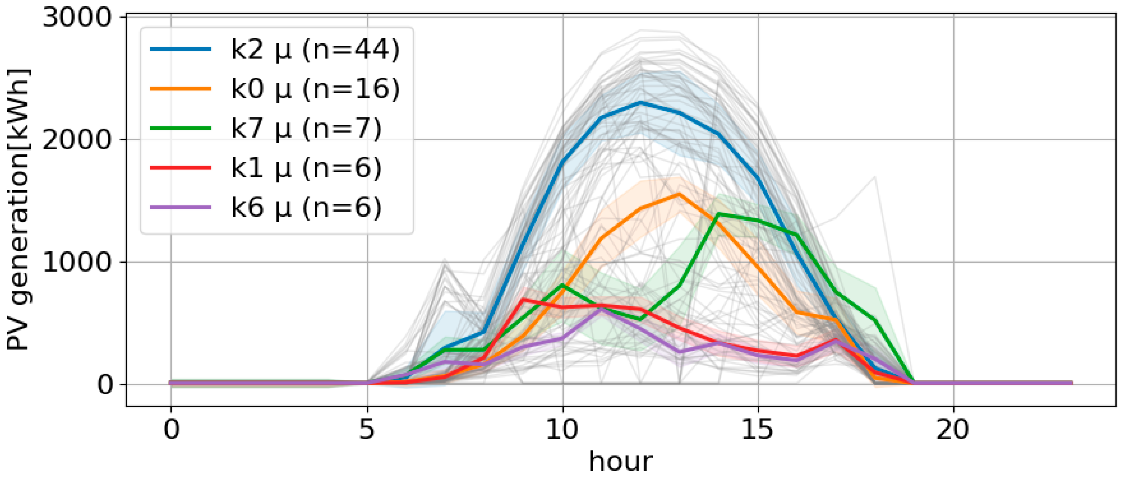
Figure 2 displays BGMM clustering results for the chosen block after magnitude normalization of daily profiles. Colored curves indicate cluster means with $\pm 1\sigma$ envelopes, and the legend reports the number of days per cluster. In this block, sharply peaked shapes around solar noon coexist with lower peaks caused by clouds and deviations. The soft responsibilities and the recency weighting obtained here are later combined into the day weights $w_d$ used in evaluation.

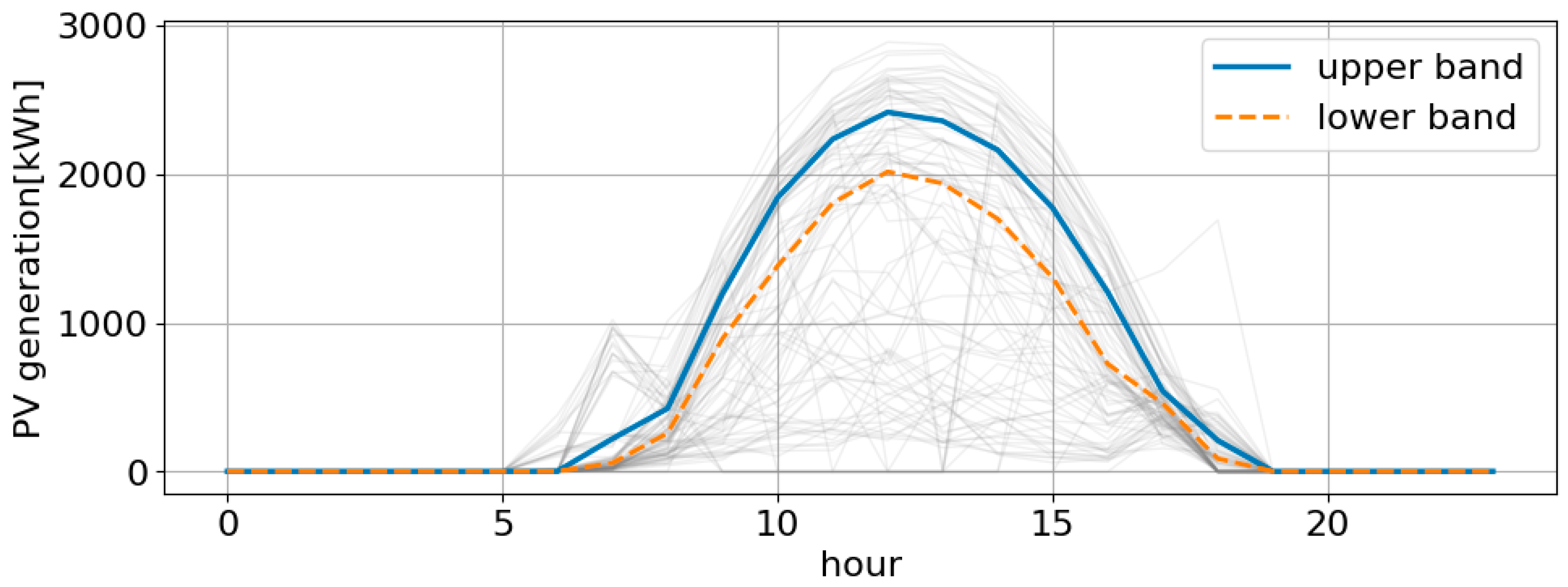
Figure 3 plots the upper and lower bands obtained by jointly optimizing $q*$ and $∆q$ with NSGA-II. In regions dominated by frequent and recent shapes the band achieves high $FA{C}_{hour}$ and stable inclusion, while a conservative upper curve restrains the upper-exceedance rate $EX$ for rare anomalous shapes.

Table 1. Validation Metrics of Representative Bands for Each Section and Block (Pyoseon Feeder).

Section	Block	$\mathit{F}\mathit{A}{\mathit{C}}_{\mathit{h}\mathit{o}\mathit{u}\mathit{r}}$	$\mathit{P}\mathit{I}\mathit{C}{\mathit{P}}_{\mathit{h}\mathit{o}\mathit{u}\mathit{r}}$	$\mathit{E}{\mathit{X}}_{\mathit{t}\mathit{o}\mathit{t}}$	$\mathit{E}{\mathit{X}}_{\mathit{r}\mathit{e}\mathit{c}\mathit{e}\mathit{n}\mathit{t}}$
Section 1	Block1	0.7864	0.4574	0.0927	0.0568
	Block2	0.8375	0.4801	0.0557	0.0555
	Block3	0.8216	0.4941	0.0493	0.0476
	Block4	0.8615	0.4901	0.0630	0.0714
	Block5	0.8936	0.5970	0.0324	0.0546
Section 2	Block1	0.7895	0.5772	0.0713	0.0493
	Block2	0.8330	0.4862	0.0740	0.0666
	Block3	0.8623	0.4922	0.0630	0.0714
	Block4	0.8758	0.5844	0.1142	0.0545
Section 3	Block1	0.8665	0.7146	0.0860	0.0769
	Block2	0.8846	0.7509	0.0920	0.1000
	Block3	0.8635	0.6977	0.0898	0.0799
	Block4	0.8120	0.6410	0.0584	0.0543
	Block5	0.8901	0.7128	0.0774	0.0869
	Block6	0.8624	0.6771	0.0883	0.0645
	Block7	0.8989	0.6829	0.1053	0.0506
Section 4	Block1	0.8202	0.6885	0.0576	0.0520
	Block2	0.8844	0.6478	0.0541	0.0513
Section 5	Block1	0.7964	0.6249	0.0909	0.0495
	Block2	0.8798	0.5857	0.0571	0.0520
Section 6	Block1	0.8072	0.5773	0.0384	0.0493
	Block2	0.8319	0.4836	0.0740	0.0666
	Block3	0.8615	0.4901	0.0630	0.0714
	Block4	0.8993	0.6020	0.0330	0.0548
Section 7	Block1	0.7579	0.5414	0.0310	0.0555
	Block2	0.8615	0.4935	0.0630	0.0714
	Block3	0.8917	0.6069	0.0402	0.0430
Section 8	Block1	0.8386	0.6568	0.0961	0.0587
	Block2	0.8772	0.7970	0.1081	0.1000
	Block3	0.8056	0.7471	0.0429	0.0540
	Block4	0.8531	0.5765	0.0586	0.0625
	Block5	0.8440	0.6358	0.0828	0.0574
	Block6	0.8825	0.6838	0.0250	0.0581
Section 9	Block1	0.7802	0.5257	0.0529	0.0555
	Block2	0.8637	0.4944	0.0630	0.0714
	Block3	0.8900	0.6077	0.0361	0.0435
Section 10	Block1	0.8398	0.6101	0.0540	0.0588
	Block2	0.8157	0.5262	0.1026	0.0000
	Block3	0.7534	0.3575	0.0673	0.0625
	Block4	0.8727	0.5151	0.0063	0.0540
Section 11	Block1	0.9448	0.9219	0.0821	0.0769
	Block2	0.8905	0.8698	0.1107	0.1000
	Block3	0.8151	0.5466	0.0980	0.0549
	Block4	0.9027	0.7113	0.0726	0.0517
Section 12	Block1	0.7830	0.5861	0.0269	0.0555
	Block2	0.8654	0.5026	0.0630	0.0714
	Block3	0.8911	0.6171	0.0371	0.0432
Average		0.8497	0.6035	0.0659	0.0605

summarizes $FA{C}_{hour}$, $PIC{P}_{hour}$, $E{X}_{tot}$, $E{X}_{recent}$ by block for the 12 sections with materially nonzero generation out of 17 sections.

Table 1 shows the block-level averages are $FA{C}_{hour}$ 0.850, $PIC{P}_{hour}$ 0.604, $E{X}_{tot}$ 0.066, and $E{X}_{recent}$ 0.061. The systematic gap between $FA{C}_{hour}$ and $PIC{P}_{hour}$ follows from weighting. $FA{C}_{hour}$ is a bilateral coverage with day weights $w_d$. It counts an hour as covered when $L_d\left(h\right)\le X_d\left(h\right)\le U_d\left(h\right)$ and normalizes by $\sum w_d$. $PIC{P}_{hour}$ computes the same inclusion condition as an unweighted mean. As a result, infrequent adverse days with heavy cloud or shading depress $PIC{P}_{hour}$ more strongly, whereas $FA{C}_{hour}$ remains higher as it emphasizes frequent recent shapes. The $EX$ metrics aggregate upper-side violations via $1\{X_d\left(h\right)\ge U_d(h\left)\right\}$ in order to monitor upward tail risk separately.

This pattern is aligned with our design goals. The design prioritizes stable representation of frequent and recent shapes while suppressing upward exceedance on rare anomalies. Operationally, the upper curve is directly connected to threshold setting, constraint tuning, and reserve margins, so keeping EX low is important. The lower curve is often crossed due to normal variability such as irradiance dips and partial shading. For this reason, widening the band to the lower side may dilute actionable information. In practice an average $PIC{P}_{hour}$ near 0.60 together with $FA{C}_{hour}$ near 0.85 and $EX$ near 0.06 indicates that the band reliably includes frequent recent shapes while sufficiently restraining upward risk. If policy prefers a higher absolute inclusion rate, one may raise the upper bound on $∆q$ or increase the constraint $PIC{P}_{hour}\ge p_{min}$ to lift $PIC{P}_{hour}$. Such changes can inflate the band, so the $EX$ metrics should be monitored jointly.

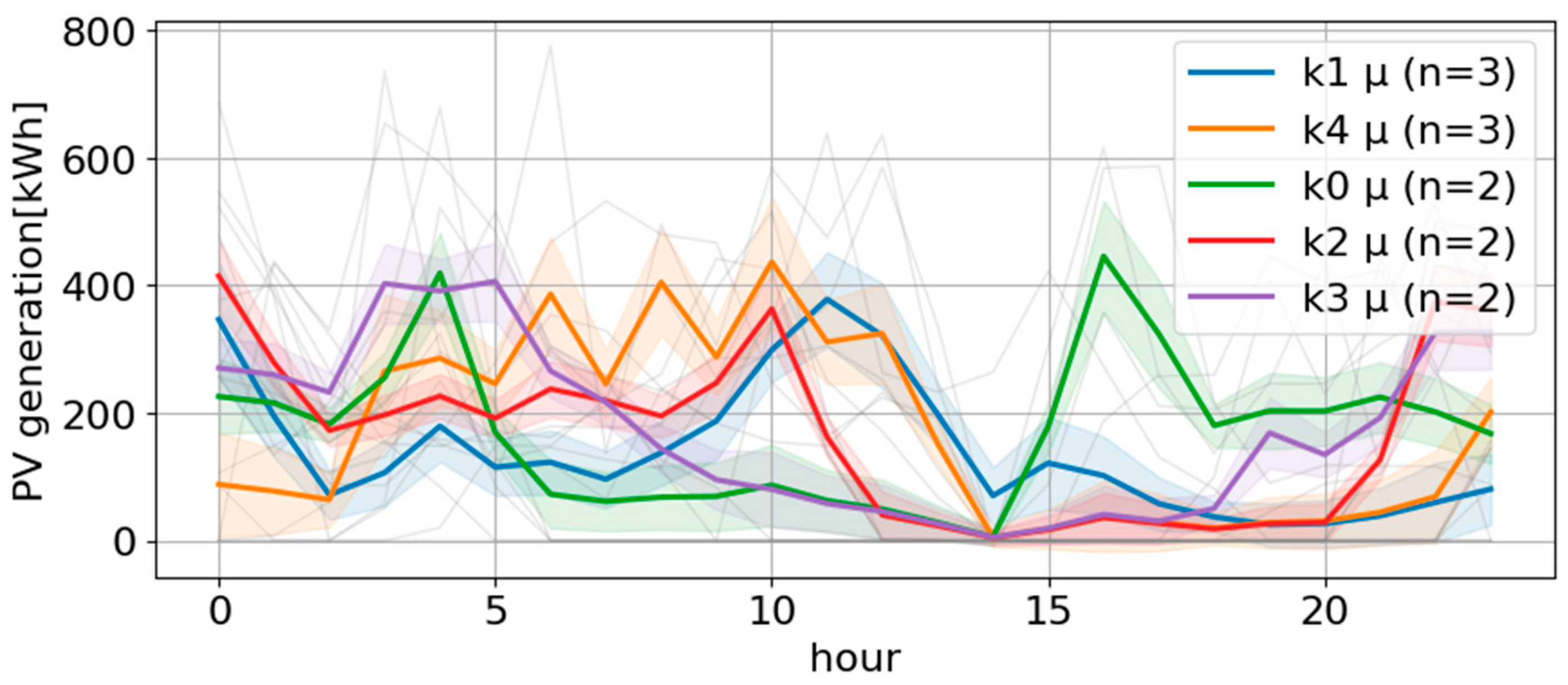
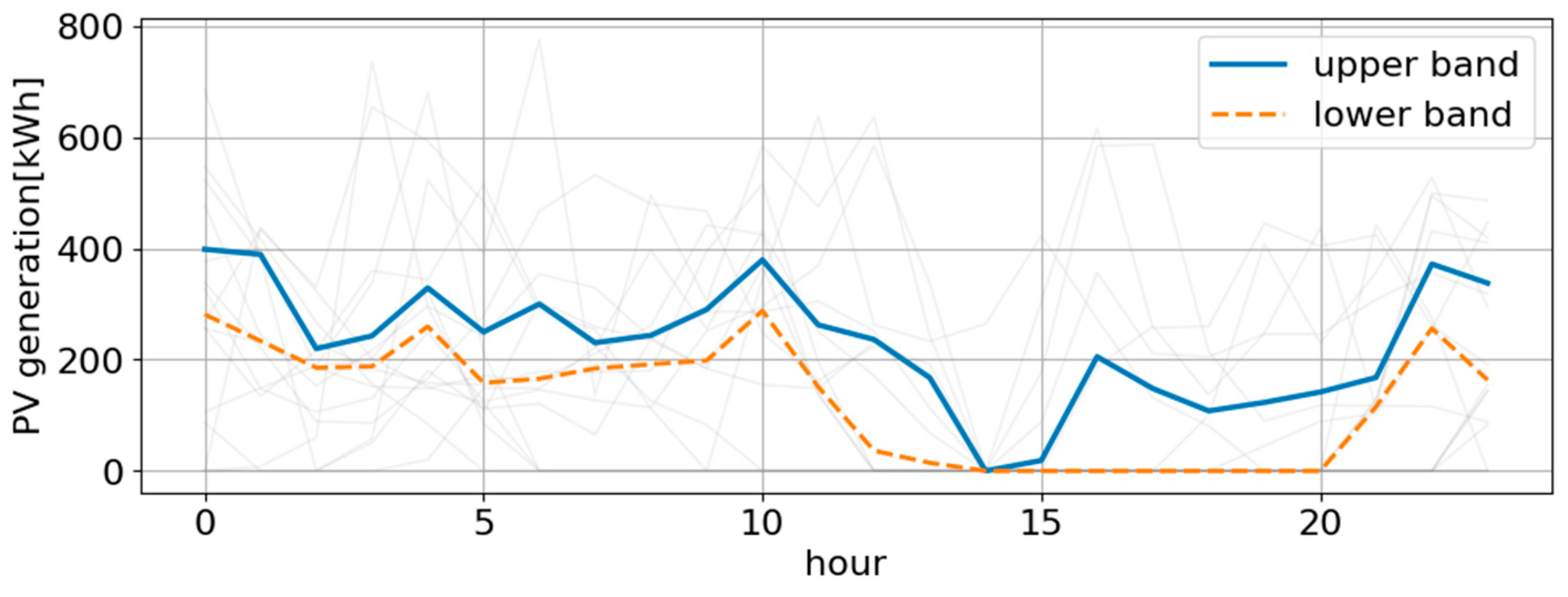
Section 10 Block 3 reports $PIC{P}_{hour}$ of 0.3575 and $FA{C}_{hour}$ of 0.7534. Figure 4 and Figure 5 indicate that multiple regimes with distinct shapes and scales coexist within this block. The proposed envelope is designed to track frequent and recent shapes and to restrain the upper tail, so it achieves tight inclusion around the dominant regime and maintains a low $EX$ value. In contrast, low-frequency regimes such as sustained midday low-output conditions or late-day spikes are included less consistently as the framework prioritizes recency and frequency rather than unconditional inclusion. This accounts for the lower $PIC{P}_{hour}$ observed for this block.

This outcome can be interpreted as an intended trade-off of the framework. The method favors recency-aligned and frequency-aligned shape fidelity over uniform inclusion across rare regimes. From an operational standpoint this block should be labeled as volatile. If a higher unconditional inclusion is required, a small relaxation such as a modest widening of the envelope or a re-segmentation of regime boundaries can be applied. At the same time the low upper exceedance supports conservative threshold setting for alarms and constraints.

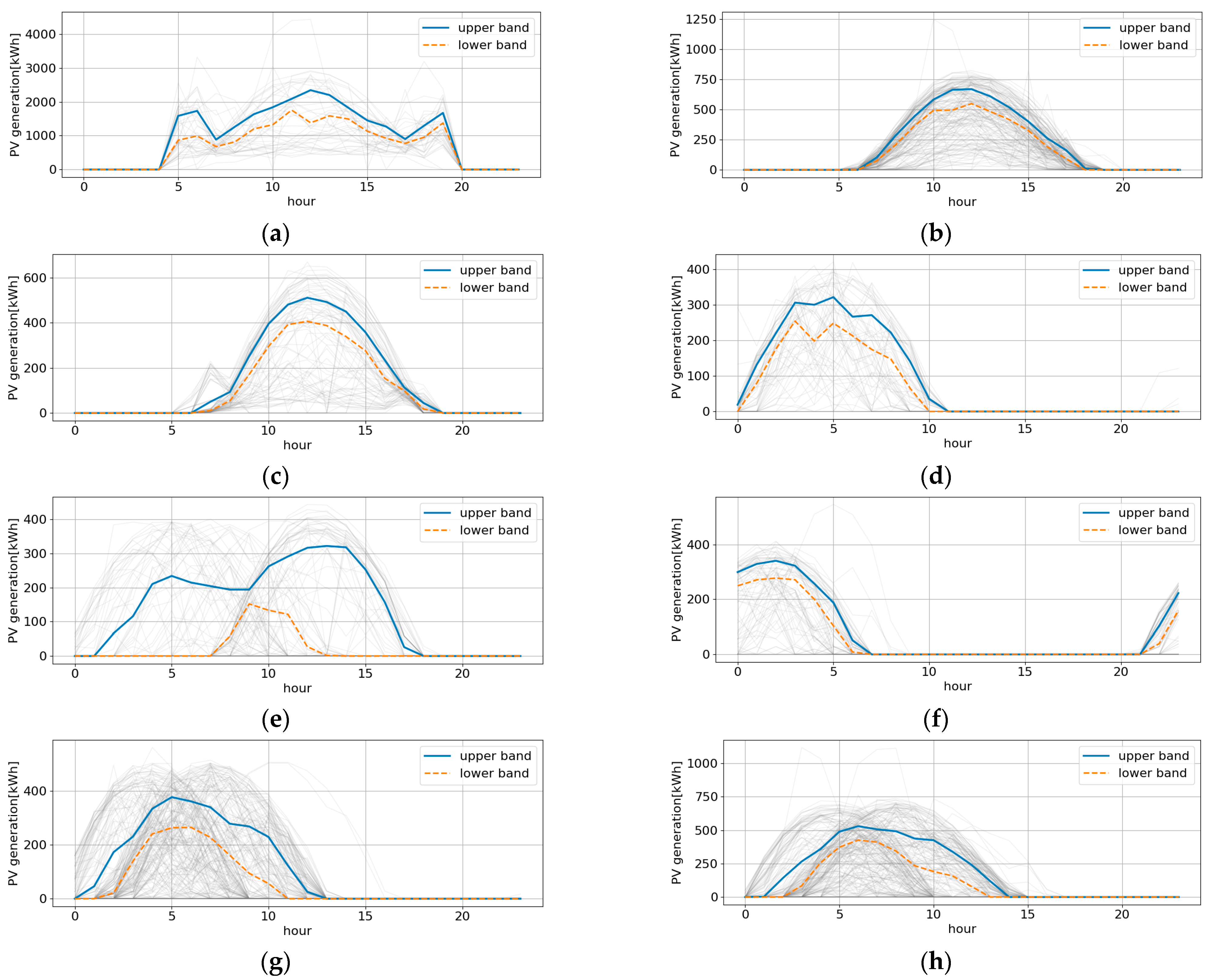
Figure 6 compares the representative bands for eight example daily profile groups from the Pyoseon feeder. Figure 6a–c correspond to regimes with a well-defined main peak (two-peak and high- or medium-output single-peak shapes). In these cases, the variance around the dominant peak is relatively small, and the gap between the upper and lower bands is narrow near the peak while gradually widening toward the edges of the active window. Figure 6d–f illustrate asymmetric or truncated profiles in which generation is concentrated in part of the day; the upper band tracks the local maxima in these regions, whereas the chosen width $∆q$ remains moderate so that the recent upper tail exceedance $EX$ stays low. Figure 6g,h show low-generation or noisy profiles with wider dispersion across days. Here, the active time window can shorten and $PIC{P}_{hour}$ may appear lower, yet representativeness is preserved in $FA{C}_{hour}$, which is tied to frequent and recent shapes. Across all eight types, the same optimization principle is applied: LSTM-AE segmentation and micro-splitting improve within-block homogeneity, BGMM responsibilities with recency weighting emphasize operationally important shapes, and NSGA-II balances band compactness with suppression of extreme upward excursions. The resulting upper curves avoid systematic underestimation or overestimation while stably capturing frequent shapes across diverse profile types.

As an additional validation, the proposed method is compared with K-Means, a widely used baseline for representative pattern extraction. While alternative clustering techniques such as GMM and DBSCAN could also be considered, K-Means was chosen due to its widespread application and simplicity. These alternative methods, however, generally fail to provide the clear upper and lower envelopes that are central to our approach, and are unlikely to outperform K-Means in the context of this task [28]. Figure 7 overlays the K-Means representative curve in blue with the upper and lower envelopes from the proposed method in orange and green. The proposed upper curve tracks the midday peak stably, while the dawn and dusk portions absorb variability with a gradual slope. The proposed lower curve accommodates normal downward fluctuations such as irradiance dips and partial shading. By contrast, the K-Means representative curve averages multiple regimes and tends to underestimate around solar noon and overestimate near sunrise and sunset. This pattern reflects the absence in K-Means of recency- and frequency-weighting as well as an explicit control on upper tail risk, making the proposed method a more robust solution for accurately capturing solar generation patterns.

The quantitative comparison is summarized in

Table 2. Validation Metrics: proposed vs. K-means (Pyoseon Feeder, Section 1, Block 1).

Model	$\mathit{F}\mathit{A}{\mathit{C}}_{\mathit{h}\mathit{o}\mathit{u}\mathit{r}}$	$\mathit{P}\mathit{I}\mathit{C}{\mathit{P}}_{\mathit{h}\mathit{o}\mathit{u}\mathit{r}}$	$\mathit{E}{\mathit{X}}_{\mathit{t}\mathit{o}\mathit{t}}$	$\mathit{E}{\mathit{X}}_{\mathit{r}\mathit{e}\mathit{c}\mathit{e}\mathit{n}\mathit{t}}$
Proposed	0.7864	0.4574	0.0927	0.0568
K-means	0.5511	0.5511	0.8019	0.6943

. Relative to the K-Means baseline, the proposed method increases $FA{C}_{hour}$ on this block by about 43%, while $PIC{P}_{hour}$ decreases by approximately 17% as the bands focus more tightly on shapes that are both frequent and recent. In other words, some coverage is intentionally given up on rare or truncated days so that the envelopes can be kept narrower and more concentrated around the dominant regimes, which is reflected as a decrease in the unweighted $PIC{P}_{hour}$ but an increase in the frequency-adjusted $FA{C}_{hour}$. At the same time, $E{X}_{tot}$ and $E{X}_{recent}$ drop from 0.8019 to 0.0927 and from 0.6943 to 0.0568, corresponding to reductions of about 88% and 92%, respectively. This trade-off indicates that the envelopes substantially strengthen inclusion of operationally relevant shapes while dramatically lowering the rate of upper-side violations, which is the key dimension for operational risk. In summary, the proposed method preserves fidelity to frequent and recent shapes and suppresses upper tail exceedance, producing operationally useful upper and lower envelopes that attain a better balance between shape representativeness and risk control than K-Means.

4. Conclusions

This study proposed a framework for constructing explainable, frequency-aware representative bands for feeder section PV output. The method combines shape-based segmentation with micro-splits, probabilistic clustering of daily profiles, and multi-objective band optimization to capture both frequent operating regimes and rare high-output events. By operating on normalized daily PV profiles and using a single set of hyperparameters across all sections, the framework is designed to be feeder-agnostic and directly reproducible without feeder-specific tuning.

Validation on one distribution feeder with section-level PV measurements shows that the resulting bands achieve high coverage of frequent and recent shapes while keeping upward exceedances small and maintaining compact width. In particular, the bands provide conservative yet frequency-consistent upper curves that align with practical planning needs at the feeder section level, where rare high outputs and operational constraints must be considered jointly. These bands are intended as probabilistic representative bands centered on frequent and recent operating regimes, with explicit information on upper tail exceedance, rather than as high-coverage uncertainty bands for the entire historical distribution. The blockwise results indicate that the framework behaves stably across sections with different PV penetration levels and orientations, supporting its use for capacity setting, reserve assessment, and maintenance planning.

At the same time, the empirical scope of this work is intentionally limited: the data come from a single year and a single feeder, and only 12 of 17 sections exhibit non-negligible PV. The present study should therefore be viewed as a proof-of-concept demonstration on a representative but constrained case rather than as a comprehensive benchmarking exercise. Extending the validation to multiple feeders, additional years, and other types of distributed resources is an important direction for future work. Further research could also explore alternative clustering and optimization schemes, as well as integration with full system-planning or operational decision tools, to assess the portability and robustness of the proposed framework under broader conditions.

References

1. International Renewable Energy Agency (IRENA). Renewable Energy Highlights, July 2025; IRENA: Abu Dhabi, United Arab Emirates, 2025. [Google Scholar]
2. Cao, W.; Zhou, J.; Zu, Q.; Zhen, J.; Huang, X. Short-Term Forecasting and Uncertainty Analysis of Photovoltaic Power Based on the FCM-WOA-BILSTM Model. Front. Energy Res. 2022, 10, 926774. [Google Scholar] [CrossRef]
3. Teichgraeber, H.; Brandt, A.R. Clustering Methods to Find Representative Periods for the Optimization of Energy Systems: An Initial Framework and Comparison. Appl. Energy 2019, 239, 1283–1293. [Google Scholar] [CrossRef]
4. Scott, I.J.; Carvalho, P.M.S.; Botterud, A.; Silva, C.A. Clustering Representative Days for Power Systems Generation Expansion Planning: Capturing the Effects of Variable Renewables and Energy Storage. Appl. Energy 2019, 253, 113603. [Google Scholar] [CrossRef]
5. Nahmmacher, P.; Schmid, E.; Hirth, L.; Knopf, B. Carpe Diem: A Novel Approach to Select Representative Days for Long-Term Power System Modeling. Energy 2016, 112, 430–442. [Google Scholar] [CrossRef]
6. Moradi-Sepahvand, M.; Tindemans, S.H. Representative Days and Hours with Piecewise Linear Transitions for Power System Planning. Electr. Power Syst. Res. 2024, 234, 110788. [Google Scholar] [CrossRef]
7. Yang, J.; Zhang, S.; Xiang, Y.; Liu, J.; Liu, J.; Han, X.; Teng, F. LSTM Auto-Encoder Based Representative Scenario Generation Method for Hybrid Hydro–PV Power System. IET Gener. Transm. Distrib. 2020, 14, 5935–5943. [Google Scholar] [CrossRef]
8. Yeganefar, A.; Amin-Naseri, M.R.; Sheikh-El-Eslami, M.K. Improvement of representative days selection in power system planning by incorporating the extreme days of the net load to take account of the variability and intermittency of renewable resources. Appl. Energy 2020, 272, 115224. [Google Scholar] [CrossRef]
9. Dalal, D.; Pal, A.; Augustin, P. Representative Scenarios to Capture Renewable Generation Stochasticity and Cross-Correlations. In Proceedings of the 2022 IEEE Power & Energy Society General Meeting (PESGM), Denver, CO, USA, 17–21 July 2022; pp. 1–5. [Google Scholar] [CrossRef]
10. Barbar, M.; Mallapragada, D.S. Representative period selection for power system planning using autoencoder-based dimensionality reduction. arXiv 2022, arXiv:2204.13608. [Google Scholar] [CrossRef]
11. Tanoto, Y.; Budhi, G.S.; Mingardi, S.F. Clustering-based assessment of solar irradiation and temperature attributes for PV power generation site selection: A case of Indonesia’s Java-Bali region. Int. J. Renew. Energy Dev. 2024, 13, 351–361. [Google Scholar] [CrossRef]
12. Liu, Y.; Sioshansi, R.; Conejo, A.J. Hierarchical clustering to find representative operating periods for capacity-expansion modeling. IEEE Trans. Power Syst. 2018, 33, 3029–3039. [Google Scholar] [CrossRef]
13. Lythcke-Jørgensen, C.E.; Münster, M.; Ensinas, A.V.; Haglind, F. A method for aggregating external operating conditions in multi-generation system optimization models. Appl. Energy 2016, 166, 59–75. [Google Scholar] [CrossRef]
14. Li, S.; Ma, H.; Li, W. Typical solar radiation year construction using k-means clustering and discrete-time Markov chain. Appl. Energy 2017, 205, 720–731. [Google Scholar] [CrossRef]
15. Tejada-Arango, D.A.; Domeshek, M.; Wogrin, S.; Centeno, E. Enhanced representative days and system states modeling for energy storage investment analysis. IEEE Trans. Power Syst. 2018, 33, 6534–6544. [Google Scholar] [CrossRef]
16. Sun, E.; Teng, X.; Zhang, X.; Strbac, G.; Pudjianto, D. Data-driven representative day selection for investment decisions: A cost-oriented approach. IEEE Trans. Power Syst. 2019, 34, 2925–2936. [Google Scholar] [CrossRef]
17. Teichgraeber, H.; Brandt, A.R. Time-series aggregation for the optimization of energy systems: Goals, challenges, approaches, and opportunities. Renew. Sustain. Energy Rev. 2022, 157, 111984. [Google Scholar] [CrossRef]
18. Fitiwi, D.Z.; Cuadra, F.; Olmos, L.; Rivier, M. A new approach of clustering operational states for power network expansion planning problems dealing with RES generation operational variability and uncertainty. Energy 2015, 90, 1360–1376. [Google Scholar] [CrossRef]
19. Yin, Y.; He, C.; Liu, T.; Wu, L. Risk-averse stochastic midterm schedule of thermal-hydro-wind system: A network-constrained clustered unit commitment approach. IEEE Trans. Sustain. Energy 2022, 13, 1293–1304. [Google Scholar] [CrossRef]
20. Prompook, T.; Jittanon, S.; Phumeesut, K.; Termritthikun, C.; Ketjoy, N.; Chamsa-Ard, W.; Meesuk, N.; Madtharad, C.; Suriwong, T. Impact of distance measures in adaptive K-means clustering on load profiles and spatial patterns of distributed substations in Thailand. Sci. Rep. 2025, 15, 21123. [Google Scholar] [CrossRef]
21. Truong, C.; Oudre, L.; Vayatis, N. Selective Review of Change Point Detection Methods. Signal Process 2020, 167, 107299. [Google Scholar] [CrossRef]
22. Sakoe, H.; Chiba, S. Dynamic Programming Algorithm Optimization for Spoken Word Recognition. IEEE Trans. Acoust. Speech Signal Process. 1978, 26, 43–49. [Google Scholar] [CrossRef]
23. Blei, D.M.; Jordan, M.I. Variational Inference for Dirichlet Process Mixtures. Bayesian Anal. 2006, 1, 121–144. [Google Scholar] [CrossRef]
24. Rasmussen, C.E. The Infinite Gaussian Mixture Model. In Advances in Neural Information Processing Systems; Solla, S.A., Leen, T.K., Müller, K.-R., Eds.; MIT Press: Cambridge, MA, USA, 2000; pp. 554–560. [Google Scholar]
25. Deb, K.; Pratap, A.; Agarwal, S.; Meyarivan, T. A fast and elitist multi objective genetic algorithm: NSGA-II. IEEE Trans. Evol. Comput. 2002, 6, 182–197. [Google Scholar] [CrossRef]
26. Rockafellar, R.T.; Uryasev, S. Conditional Value-at-Risk for General Loss Distributions. J. Bank. Financ. 2002, 26, 1443–1471. [Google Scholar] [CrossRef]
27. Khosravi, A.; Nahavandi, S.; Creighton, D.; Atiya, A.F. Comprehensive Review of Neural Network-Based Prediction Intervals and New Advances. IEEE Trans. Neural Netw. 2011, 22, 1341–1356. [Google Scholar] [CrossRef]
28. Gokcesu, K.; Gokcesu, H. Nonparametric Extrema Analysis in Time Series for Envelope Extraction, Peak Detection and Clustering. arXiv 2021, arXiv:2109.02082. [Google Scholar] [CrossRef]
Figure 1. Daily PV Generation and Block Segmentation (Pyoseon Feeder, Section 1).
Energies 18 06134 g001
Figure 2. BGMM-based Cluster Prototypes (Pyoseon Feeder, Section 1, Block 1).
Energies 18 06134 g002
Figure 3. Optimized representative PV generation Bands (Pyoseon Feeder, Section 1, Block 1).
Energies 18 06134 g003
Figure 4. Section 10–Block 3 clustering and cluster prototypes (Pyoseon Feeder).
Energies 18 06134 g004
Figure 5. Section 10–Block 3 optimized envelope with upper and lower bands (Pyoseon Feeder).
Energies 18 06134 g005
Figure 6. Representative generation bands for eight typical daily profile types on the Pyoseon feeder: (a) two-peak profiles, (b) high-output single-peak profiles, (c) medium-output single-peak profiles, (d) single-peak profiles with midday distortion, (e) extended-plateau profiles, (f) morning-dominated or truncated profiles, (g) low-amplitude diffuse profiles, and (h) noisy high-variance profiles.
Energies 18 06134 g006
Figure 7. Comparison results with K-Means (Pyoseon Feeder, Section 1, Block 1).
Energies 18 06134 g007