Probabilistic Analysis of Solar and Wind Energy Potentials at Geographically Diverse Locations for Sustainable Renewable Integration

Abstract

The use of conventional fuel sources from the Earth to generate electrical power leads to several environmental issues such as carbon emissions and ozone depletion. Energy generation from renewable energy sources is one of the most affordable and cleanest techniques. However, the generation of power from non-conventional sources like solar and wind requires the examination of established locations where these resources are plentiful and easily accessible. In this study, an investigation of solar and wind is performed at five different sites in various locations in India. For this examination, data on solar irradiance ($\mathrm{W}/{\mathrm{m}}^2$) and wind speed ($\mathrm{m}/\mathrm{s}$) is taken from the “NASA POWER DAV v.2.5.22” Data Access Viewer created by NASA. The data for solar and wind was taken at hourly intervals. The period of the investigation was ten years, i.e., from January 2014 to December 2023. The solar and wind potential analysis was performed in a probabilistic way to determine the parameters that support the installation of solar–PV panels and wind energy generators at the examined sites for the generation of power from these spontaneously available sources, respectively. To examine the potential of solar and wind sites, the Beta and Weibull probability distribution function (PDF) was used. The parameter estimation of the Beta and Weibull PDF was performed via the Maximum Likelihood method. The chosen method is known for its accuracy and efficiency in handling large datasets. Some key performance prediction indicators were analyzed for the investigated solar and wind locations. The findings provide valuable insights that support renewable energy planning and the optimal design of hybrid power systems.

1. Introduction

The generation of electrical power from renewable energy sources has become a reasonable aim, owing to their non-polluting nature and carbon-free emissions. Currently, worldwide communities need reliable and cost-effective power generation to meet their energy demands with the most affordable options. India holds enormous potential for renewable power generation, especially from solar and wind energy, due its significant size and various climatic circumstances. As the country is projected to experience an upsurge in electricity demand due to rapid industrialization and urbanization, India has set the ambitious target of producing energy from renewable energy resources. As per the report from the Ministry of New and Renewable Energy (MNRE), the country aims to achieve a capacity of 500 GW by 2030 from non-conventional sources, of which solar and wind are projected to be the foremost contributors [1]. Thus, there is a need to identify the most feasible locations for the precise assessment of solar and wind energy potential. These evaluations of resource potential will facilitate system optimization, minimize financial risks, and ensure the long-term sustainability of renewable energy projects.

India receives annual average solar radiation of approximately 4–7 $\mathrm{k}\mathrm{W}/{\mathrm{m}}^2/\mathrm{d}\mathrm{a}\mathrm{y}$ across latitudes 8°4′ and 37°6′ N, making it the most solar-rich country in the world, and most states in India have high exposure to wind due to their coastal proximity and wind flow regime [2,3]. Combining solar and wind energy supports standalone hybrid systems by reducing intermittency and improving grid stability through their complementary availability.

M. Sumair et al. [4] assessed the feasibility of wind energy projects in southern Punjab, highlighting their role in promoting renewable energy and decreasing reliance on fossil fuels. The analysis used a two-parameter Weibull distribution with wind speed data from 11 locations across the region. Maisam Wahbah et al. [5] introduced an innovative method that aimed to eradicate the bias that is generally found in traditional cross-validation procedures by probabilistically modeling the solar and wind energy sources crucial to renewable energy prediction and management. Lintong Liu et al. [6] evaluated the performance of solar-, wind-, and hydrogen-based hybrid power systems using several analytical methods to measure system performance, attaining energy security and decreasing carbon discharges. Meskiana Boulahia et al. [7] proposed a comprehensive engineering and statistical approach for solar examination to assess both geographical and technical potential. Madjid Chikh et al. [8] conducted a qualitative and quantitative study in the Oran, which is located in Algeria and has limited solar potential, and estimated the precision of their model using statistical indicators such as mean bias error, root mean squared error, and t-statistics. Abdulkarim et al. [9] performed frequency distribution analyses for solar and wind energy resources using various distribution functions. For solar radiation modeling, Weibull, Logistics, Lognormal, Beta, and Gamma were examined, and for wind speed modeling, Weibull, Rayleigh, and Gamma distribution functions were examined, respectively. After performing statistical tests like Kolmogorov–Smirnov, Anderson–Darling, and Chi-Square tests to judge the best-fitted distributions, it was observed that Beta is the most suitable for solar and Weibull is the best for wind potential investigations. C. Ojeda Avila et al. [10] demonstrated the accuracy of the Angstrom–Prescott linear regression model and the Bird and Hulstrom approach in enhancing solar energy utilization across different conditions. Additionally, Weibull and Rayleigh distribution functions were employed to characterize wind resource variability. Vadim Manusov et al. [11] assisted in analyzing the unpredictability of renewable energy sources, and suggested a practical explanation for refining the certainty of energy generation from wind and solar sources. D. H. Didane et al. [12] used a two-parameter Weibull distribution to assess the wind characteristics of potential sites by examining the ten-year data from 2010 to 2019 in the Chittagong division of Bangladesh. Piotr Wais [13] compared the three-parameter Weibull distribution function with the two-parameter function and found that the three-parameter distribution was better for wind speeds below 2 m/s with a high percentage of null winds. Amit Kumar Yadav et al. [14] analyzed several statistical techniques to determine the parameters of the Weibull distributions for wind potential inspections at different sites in Andhra Pradesh. F. Youcef Ettoumi et al. [15] highlighted the efficacy of Beta distribution for inspecting solar data in Algeria for the integration of solar energy in the future. M. Kolhe [16] presented the solar radiation utilization in assessing system performance and enhancing strategy by developing the relationships between the photovoltaic array and battery capacity in standalone solar systems. Ihaddadene Razika et al. [17] considered several distribution functions like Weibull, Gamma, Normal, Logistic, Lognormal, and Loglogistic functions to analyze the occurrence of solar irradiance; some statistical prediction parameters like correlation coefficient, root mean square error, mean bias error, and mean absolute bias error were evaluated to verify the efficacy of each model under investigation. M. Kolhe et al. [18] designed a solar-powered motor system that works effectively in variable situations and analyzed the system’s working productivity, highlighting the importance of solar intensity and temperature on performance. A. Rathore et al. [19] proposed a hybrid system based on the probabilistic modeling of solar and wind energy sources for which the author used Beta and Weibull distribution functions, respectively, to incorporate the intermittency along with pump storage hydro for reliability assessment. In reference [20], the author indicated the optimal sizing and placement of solar and wind with gravity energy storage for enhancing system performance and reducing energy losses by improving the voltage profile.

The precise modeling of solar irradiance and wind speed is essential for the design, forecasting, and optimization of renewable energy systems. Based on the literature, the Beta distribution aligns well with normalized solar radiation data and effectively represents asymmetric and skewed patterns commonly observed across diverse geographical regions. It also offers greater flexibility, lower RMSE values, and superior statistical fitting compared with other distribution functions such as Normal, Gamma, and Lognormal distributions [21]. For wind potential assessment, the Weibull distribution is preferred due to its greater adaptability relative to the Rayleigh distribution (which has a fixed shape), the Normal distribution (which is unsuitable for skewed wind data), and the Lognormal distribution (which is more complex and less stable). The Weibull distribution is widely chosen because it can represent a broad range of wind characteristics through adjustable shape and scale parameters and provides a direct analytical expression for wind power density (WPD) [22,23]. Therefore, among the various probability distribution functions, the Beta PDF (for solar irradiance) and the Weibull PDF (for wind speed) are recognized as the most effective, flexible, and practical choices for probabilistic renewable energy assessments.

The key objectives of this study include the following:

• Assessing a long-term metrological dataset of renewable energy, i.e., solar (solar irradiance) and wind (wind speed) energy, from 2014 to 2023.
• Conducting a probabilistic and statistical examination of solar and wind using Beta and Weibull PDF, respectively, to incorporate their intermittency.
• Evaluating the prediction parameters to support the potential investigation of five locations.
• Estimating supportive tests and parameters for fitting the distribution function for site analysis.

The individuality of this study encompasses three major aspects. First, the study utilizes a decade-long (2014–2023) high-resolution hourly dataset from Data Access Viewer v2.5.22 to evaluate both solar and wind resources simultaneously across geographically diverse Indian sites. Second, the study applies a probabilistic modeling framework combining Beta and Weibull distributions, enabling a statistically robust assessment of variability, reliability, and goodness-of-fit performance indicators (RMSE, MAPE, MBE, and K–S statistics). The simultaneous investigation of solar and wind has not been conducted previously in a probabilistic way in any of the reviewed studies. Third, the research decodes the statistical findings into engineering and planning insights by linking distribution parameters to wind power density (WPD) classes, maximum energy-carrying wind speeds ($V_{me}$), and solar PV sizing implementations. These fundamentals collectively advance beyond previous regional studies that examined shorter time periods or focused on a single energy source, offering a more comprehensive framework for hybrid solar–wind site selection and system planning in the Indian context.

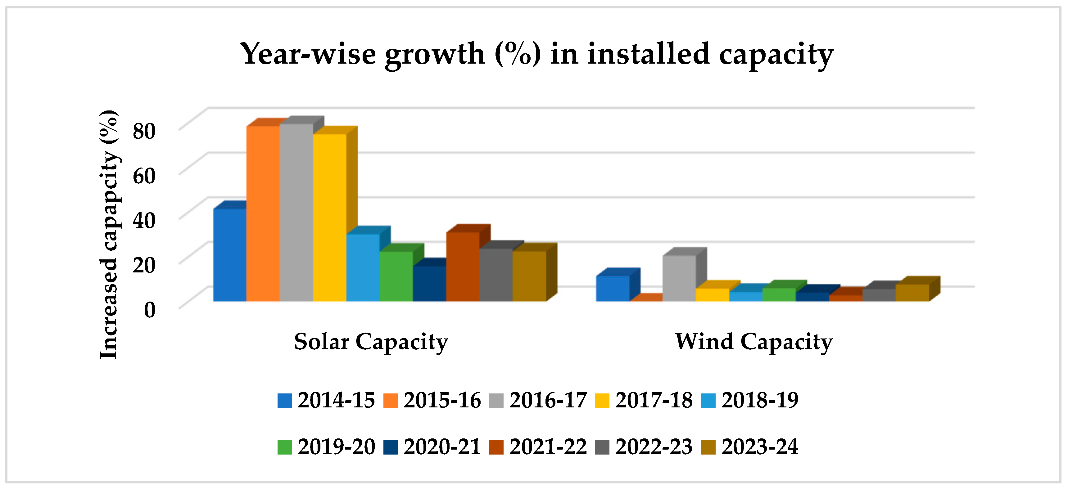
Figure 1 represents the incremental development in solar and wind power installed capacity for the last decade (2014-15 to 2023-24) in India [3]. The total installed capacity from renewable sources (which includes wind, solar, small-hydro, and biomass power) was 143.65 GW as of 31 March 2024. The share of solar was 3.99 GW as of March 2015, which is approximately 9.97% of the total renewable capacity; this increased to 81.81 GW, which is almost 57% of the total renewable installed capacity. Similarly, wind capacity as of March 2015 was 23.44 GW (58.54% of total renewable capacity), which increased to 45.89 GW (31.95% of total renewable capacity). This represents a huge increment of 1950.30% for solar and 95.78% for wind from 2014 to 2024.

Figure 1. Incremental growth of solar and wind capacity in India from 2014 to 2024 [3].

Figure 1. Incremental growth of solar and wind capacity in India from 2014 to 2024 [3].

Figure 2 illustrates the renewable energy installed capacity of ten nations as of 31 December 2023 [24]. China leads with the highest capacity of 1453.7 GW, whereas India has the fourth-largest installed capacity of renewable energy in world with 175.93 GW. These top ten countries contribute around 73.15% of the total global renewable capacity.

Figure 2. Collective renewable energy installed capacity of 10 leading nations up to 31 December 2023 [24].

Figure 2. Collective renewable energy installed capacity of 10 leading nations up to 31 December 2023 [24].

2. Site Description

This analysis was carried out to identify the most suitable locations for evaluating solar and wind potential. Five locations from different Indian states were selected for examination and their names, states, and geographical coordinates are provided in

Table 1. Site information for solar and wind potential investigation.

S. No	Name of the Site	State (Country)	Coordinates		Elevation (Meters)	Study Period
			Latitude	Longitude
1	Kutch District	Gujarat, India	23.79° N	68.70° E	4.49	2014–2023
2	Jaisalmer District	Rajasthan, India	27.02° N	70.52° E	173.40	2014–2023
3	Davanagere District	Karnataka, India	14.47° N	75.92° E	597.40	2014–2023
4	Rewa District	Madhya Pradesh, India	24.53° N	81.29° E	329.82	2014–2023
5	Anantapur District	Andhra Pradesh, India	14.55° N	77.37° E	447.83	2014–2023

. The study covers a ten-year period from 2014 to 2023, using hourly solar and wind data. The availability of this large dataset enables more accurate assessments and improves the reliability of forecasts for establishing renewable energy-based power generation plants.

3. Distribution Functions for Probabilistic Analysis for Solar and Wind Potential Investigation

A review of the literature shows that several distribution functions—including the Normal, Lognormal, Beta, Weibull, Rayleigh, and Gamma distributions—have been used for the probabilistic analysis and potential assessment of solar irradiance and wind speed. The findings consistently indicate that the Beta and Weibull distributions are the most suitable representations for solar and wind energy resources, respectively, due to the various advantages outlined earlier.

3.1. Beta Probability Distribution Function

Beta PDF is a continuous density function used to analyze the random behavior of a variable that lies between a finite interval [0, 1]. This PDF is mostly used by investigators for the prediction and modeling of solar irradiance. In the modeling of this Beta PDF, solar irradiance from the sun is considered as a random variable and is scaled down between 0 to 1 by dividing the actual irradiance with the maximum available irradiance for a particular location. Later, this scaled value can be converted to an actual value of irradiance by multiplying it by the maximum available solar irradiance. This PDF is extremely flexible in nature owing to the ability to adjust its shape, such bell-shaped, U-shaped, uniform or skewed. Therefore, it is a great choice for demonstrating solar irradiance while integrating intermittency [23].

$$f_B\left(s,\alpha ,\beta \right)={\displaystyle \frac{s^{\left(\alpha -1\right)}\cdot {\left(1-s\right)}^{\left(\beta -1\right)} }{B\left(\alpha , \beta \right)}} \mathrm{for} 0\le s\le 1$$

(1)

$$\mathrm{w}\mathrm{h}\mathrm{e}\mathrm{r}\mathrm{e} B\left(\alpha , \beta \right)={\int }_0^1{t}^{\alpha -1}{\left(1-t\right)}^{\beta -1}dt={\displaystyle \frac{\Gamma \left(\alpha \right)\cdot \Gamma \left(\beta \right)}{\Gamma \left(\alpha +\beta \right)}}$$

(2)

$$\mathrm{a}\mathrm{n}\mathrm{d} \alpha >0,\mathrm{and} \beta >0$$

$$s=\mathrm{s}\mathrm{o}\mathrm{l}\mathrm{a}\mathrm{r} \mathrm{i}\mathrm{r}\mathrm{r}\mathrm{a}\mathrm{d}\mathrm{i}\mathrm{n}\mathrm{a}\mathrm{c}\mathrm{e} (\mathrm{k}\mathrm{W}/{\mathrm{m}}^2)$$

$$f_B\left(s\right)=\mathrm{f}\mathrm{u}\mathrm{n}\mathrm{c}\mathrm{t}\mathrm{i}\mathrm{o}\mathrm{n} \mathrm{r}\mathrm{e}\mathrm{p}\mathrm{r}\mathrm{e}\mathrm{s}\mathrm{e}\mathrm{n}\mathrm{t}\mathrm{i}\mathrm{n}\mathrm{g} \mathrm{B}\mathrm{e}\mathrm{t}\mathrm{a} \mathrm{d}\mathrm{i}\mathrm{s}\mathrm{t}\mathrm{r}\mathrm{i}\mathrm{b}\mathrm{u}\mathrm{t}\mathrm{i}\mathrm{o}\mathrm{n}$$

$$\alpha , \beta =\mathrm{B}\mathrm{e}\mathrm{t}\mathrm{a} \mathrm{P}\mathrm{D}\mathrm{F} \mathrm{p}\mathrm{a}\mathrm{r}\mathrm{a}\mathrm{m}\mathrm{e}\mathrm{t}\mathrm{e}\mathrm{r}\mathrm{s}$$

$$\Gamma =\mathrm{G}\mathrm{a}\mathrm{m}\mathrm{m}\mathrm{a} \mathrm{f}\mathrm{u}\mathrm{n}\mathrm{c}\mathrm{t}\mathrm{i}\mathrm{o}\mathrm{n}$$

The expression for the mean $\left({\mu }_B\right)$, variance (${{\sigma }_B}^2$), and standard deviation (${\sigma }_B$) for the Beta distribution can be specified by Equations (3), (4), and (5), respectively:

$${\mu }_B= {\displaystyle \frac{\alpha }{\alpha +\beta }}$$

(3)

$${{\sigma }_B}^2={\displaystyle \frac{\alpha \beta }{(\alpha +\beta {+1\left)\right(\alpha +\beta )}^2}}$$

(4)

$${\sigma }_B=\sqrt{{\displaystyle \frac{\alpha \beta }{(\alpha +\beta {+1\left)\right(\alpha +\beta )}^2}} }$$

(5)

Parameter Estimation by Maximum Likelihood Estimation

The parameters of the Beta function can be calculated using several available techniques like Method of Moments, Bayesian estimation, L-moments, Maximum Likelihood estimation, and Log-Cumulants. Maximum Likelihood estimation is capable of handling larger samples with high accuracy and it is statistically more effective and reliable for parameter estimation than others [25,26].

Let us assume a random sample ($X_1, X_2, X_3,\dots \dots X_n$).

The likelihood function for the Beta function can be given as

$$\log L\left(\alpha ,\beta |X\right)=\left(\alpha -1\right){\sum }_{q=1}^m\log X_q+\left(\alpha -1\right){\sum }_{q=1}^m\log {(1-X}_q)-n\log B\left(\alpha ,\beta \right)$$

(6)

Now we have

$${\displaystyle \frac{\mathit{\partial }\log L\left(\alpha ,\beta |X\right)}{\mathit{\partial }\alpha }}={\sum }_{q=1}^m\log X_q-n{\displaystyle \frac{\mathit{\partial }\log B\left(\alpha ,\beta \right)}{\mathit{\partial }\alpha }}$$

(7)

$${\displaystyle \frac{\mathit{\partial }\log L\left(\alpha ,\beta |X\right)}{\mathit{\partial }\beta }}={\sum }_{q=1}^m\log \left(1-X_q\right)-n{\displaystyle \frac{\mathit{\partial }\log B(\alpha ,\beta )}{\mathit{\partial }\beta }}$$

(8)

Equations (7) and (8) are equated to zero to obtain the parameter equation with respect to Maximum Likelihood estimates.

For numerical estimation, the Newtons Rapson method is applied, for which partial derivative is essential.

$${\displaystyle \frac{\mathit{\partial }B(\alpha ,\beta )}{\mathit{\partial }\alpha }}=-\mathsf{\Psi }\left(\alpha +\beta \right)+\mathsf{\Psi }\left(\alpha \right)$$

(9)

$\mathrm{w}\mathrm{h}\mathrm{e}\mathrm{r}\mathrm{e} \mathsf{\Psi }\left(\alpha \right)= {\displaystyle \frac{\mathit{\partial }\log \Gamma \alpha }{\mathit{\partial }\alpha }}$, and the Digamma function is

$${\displaystyle \frac{\mathit{\partial }B(\alpha ,\beta )}{\mathit{\partial }\beta }}=-\mathsf{\Psi }\left(\alpha +\beta \right)+\mathsf{\Psi }\left(\alpha \right)$$

(10)

$${\displaystyle \frac{{\mathit{\partial }}^{2}B(\alpha ,\beta )}{\mathit{\partial }{\alpha }^2}}=-{\mathsf{\Psi }}_1\left(\alpha +\beta \right)+{\mathsf{\Psi }}_1\left(\alpha \right)$$

(11)

$\mathrm{w}\mathrm{h}\mathrm{e}\mathrm{r}\mathrm{e} {\mathsf{\Psi }}_1\left(\alpha \right)= {\displaystyle \frac{{\mathit{\partial }}^2\log \Gamma \alpha }{\mathit{\partial }{\alpha }^2}}$, and the Trigamma function is

$${\displaystyle \frac{{\mathit{\partial }}^{2}B(\alpha ,\beta )}{\mathit{\partial }{\beta }^2}}=-{\mathsf{\Psi }}_1\left(\alpha +\beta \right)+{\mathsf{\Psi }}_1\left(\alpha \right)$$

(12)

This will result in finding $\alpha \mathrm{a}\mathrm{n}\mathrm{d} \beta$.

3.2. Weibull Probability Distribution Function

The Weibull PDF, a continuous distribution that reflects the fluctuating behavior of wind speed, is widely regarded as the preferred model for probabilistic wind potential assessment. Equation (13) represents the Weibull probability distribution function [23,27,28].

$$f_w\left(v\right)={\displaystyle \frac{k}{c}}{\ast \left({\displaystyle \frac{v}{c}}\right)}^{k-1}{e}^{-{\left({\displaystyle \frac{v}{c}}\right)}^K} \mathrm{for} v > 0, c > 1 \mathrm{and} k > 1$$

(13)

where

k is the shape and c is the scale parameter of Weibull probability distribution function;

v stands for varying wind speed $(\mathrm{m}/\mathrm{s})$;

k has no unit, whereas c has a similar dimension to wind speed $(\mathrm{m}/\mathrm{s})$.

The cumulative distribution function ${(F}_w\left(v\right)$) of the corresponding function can be attained by capturing the inverse of Equation (6) and can be described as

$$F_w\left(v\right)={\int }_0^v{f}_w\left(v\right) dv$$

(14)

Upon the simplification of Equation (7), $F_w\left(v\right)$ can be rewritten as

$$F_w\left(v\right)=1-e^{{-\left({\displaystyle \raisebox{1ex}{$v$}\!\left/ \!\raisebox{-1ex}{$c$}\right.}\right)}^k}$$

(15)

The mean (${\mathrm{\mu }}_w)$, variance (${{\sigma }^2}_w$), and standard deviation (${\mu }_w$) of the corresponding distribution in terms of parameter can be respectively stated as

$${\mu }_w=c \Gamma \left(1+{\displaystyle \frac{1}{k}}\right)$$

(16)

$${\sigma }_w^2=c^2\left[\Gamma \left(1+{\displaystyle \frac{2}{k}}\right)-{\Gamma }^2\left(1+{\displaystyle \frac{1}{k}}\right)\right]$$

(17)

$${\sigma }_w=c\sqrt{\left[\Gamma \left(1+{\displaystyle \frac{2}{k}}\right)-{\Gamma }^2\left(1+{\displaystyle \frac{1}{k}}\right)\right]}$$

(18)

Parameter Estimation via Maximum Likelihood Method

There are numerous existing approaches through which the parameters of this distribution can be obtained. Some of the popularly known methods are the Method of Moment, Empirical Method of Justus, Empirical Method of Lysen, Maximum Likelihood, the Energy Pattern Factor method, and Standard Deviation. Each method has its own criteria, limitations, advantages, assumptions, accuracy, complexity, and computational burden. This study involves a huge dataset covering a decade of information. The wind speed data was collected at consecutive hourly intervals over 10 years, with nearly 87,600 points for each investigated site. Therefore, it is very important to understand the previous history of the used method. The Maximum Likelihood method can cope with massive datasets while estimating parameters precisely and truthfully, and can incorporate the intermittency of the dataset.

This procedure is quite difficult and requires much repetition to evaluate the parameters of the distribution function. A well-known likelihood function employs a time series structure of wind speed statistics, giving rise to the term Maximum Likelihood. This technique guesses the unnoticed limitations based on observable parameters [27,28].

Wind speed is utilized as a random variable to evaluate the parameters of the Weibull distribution function, as shown in Equation (13). Assume that $\left(v_1,v_2,v_3,\dots \dots .v_n\right)$ are the wind speed trials of the selected function and their equivalent likelihood function $L\left(K,C,v_1,v_2,v_3,\dots \dots .v_n\right)$ can be signified as

$$L\left(K,C,v_1,v_2,v_3,\dots \dots .v_n\right)={\prod }_{r=1}^{n}f(K,C,v_r)$$

(19)

Applying log for simplification,

$$\ln L={\sum }_{r=1}^n\ln 〈f\left(v_r\right)〉$$

(20)

We can differentiate the above equation to obtain k and c:

$${\displaystyle \frac{\mathit{\partial }\ln L}{\mathit{\partial }K}}=0$$

(21)

$${\displaystyle \frac{\mathit{\partial }\ln L}{\mathit{\partial }C}}=0$$

(22)

Upon simplification of Equations (21) and (22), the values K and C can be individually denoted as

$$k={\left({\displaystyle \frac{{\sum }_{r=1}^n{v^K}_r\ln v_r}{{\sum }_{r=1}^n{v^K}_r}}-{\displaystyle \frac{{\sum }_{r=1}^n\ln v_r}{n}}\right)}^{-1}$$

(23)

$$c={〈{\displaystyle \frac{1}{n}}{\sum }_{r=1}^n{\left(v_r\right)}^K〉}^{{\displaystyle \frac{1}{K}}}$$

(24)

where n is the total wind speed count and ${\mathrm{v}}_{\mathrm{r}}$ is the measured wind speed for the r interval.

4. Statistical Characteristics for Renewable Assessment

4.1. Skewness

This statistical quantity defines the unevenness of a particular PDF around its mean value. It tells us about the direction in which the side of a PDF is stretched out or which side has a longer tail. If the value of skewness is zero, its tail is equally divided. A positive value represents a longer right tail, whereas a negative value indicates a longer left tail. This factor helps in model selection, risk analysis, and renewable energy planning. The skewness for Beta (Equation (25)) and Weibull (Equation (26)) distribution is designated below in terms of their parameters.

$${\gamma }_B={\displaystyle \frac{2(\beta -\alpha )\sqrt{\alpha +\beta +1}}{\left(\alpha +\beta +2\right)\sqrt{\alpha \beta }}}$$

(25)

$${\gamma }_w={\displaystyle \frac{\Gamma \left(1+\frac{3}{k}\right)c^3-3{\mu }_w{\sigma }_w^2-{{\mu }_w}^3}{{\sigma }_w^3}}$$

(26)

4.2. Kurtosis

This statistical quantity describes the sharpness and flatness of a PDF with respect to normal distribution. It helps distinguish between highly concentrated and evenly spread random quantities (like solar irradiance and wind speed with respect to solar and wind analysis, respectively) over the assessment period. The expression for kurtosis with respect to Beta (Equation (27)) and Weibull (Equation (28)) are shown below.

$${\kappa }_B={\displaystyle \frac{6 \left[{\left(\alpha -\beta \right)}^2\left(\alpha +\beta +1\right)-\alpha \beta \left(\alpha +\beta +2\right)\right]}{\alpha \beta \left(\alpha +\beta +2\right)\left(\alpha +\beta +3\right)}}$$

(27)

$${\kappa }_w=c^4\left[\Gamma \left(1+{\displaystyle \frac{4}{k}}\right)-4{\mu }_w\Gamma \left(1+{\displaystyle \frac{3}{k}}\right)+6{{\mu }_w}^2\Gamma \left(1+{\displaystyle \frac{2}{k}}\right)-3{{\mu }_w}^4\right]$$

(28)

4.3. Coefficient of Variation

Coefficient of variation (CV) is the normalized degree of dispersal of a PDF. It helps analyze the variability of a distribution with respect to mean value. A low value (nearly zero) of this parameter indicates more stable distribution, whereas a high value corresponds to more variability. The CV for Beta and Weibull is illustrated in Equation (29) and Equation (30), respectively.

$${CV}_B={\displaystyle \frac{{\mu }_B}{{\sigma }_B}}=\sqrt{{\displaystyle \frac{\beta }{\alpha \left(\alpha +\beta +1\right)}}}$$

(29)

$${CV}_w={\displaystyle \frac{{\mu }_w}{{\sigma }_w}}={\displaystyle \frac{\sqrt{\Gamma \left(1+\frac{2}{k}\right)-{\left(\Gamma \left(1+\frac{1}{k}\right)\right)}^2}}{\Gamma \left(1+\frac{1}{k}\right)}}$$

(30)

4.4. Mode

This statistical parameter gives practical insight to the most likely value of a random variable like solar irradiance and wind speed with respect to solar and wind potential assessment. The mode (Mo) for Beta and Weibull is shown below in Equation (31) and Equation (32), respectively:

$${MO}_B= {\displaystyle \frac{\alpha -1}{\alpha +\beta -2}}; \alpha , \beta >1$$

(31)

$${MO}_w=c {\left({\displaystyle \frac{k-1}{k}}\right)}^{{\displaystyle \raisebox{1ex}{$1$}\!\left/ \!\raisebox{-1ex}{$k$}\right.}}; k>1$$

(32)

5. Performance Prediction Pointers

5.1. Root Mean Square Error (RMSE)

RMSE is one of the key performance metrics used to evaluate a regression model. It represents the mean difference between the predicted values generated by the statistical model and the corresponding actual values. This indicator reflects the accuracy of the model’s predictions and is particularly useful for forecasting renewable energy integration at potential sites. A smaller value of this metric—approaching zero—indicates a more precise and reliable model.

5.2. Mean Absolute Percentage Error (MAPE)

This metric calculates the absolute percentage deviation between the true and predicted values, enabling the evaluation of the model’s ability to reflect real-world performance.

5.3. Mean Bias Error (MBE)

An optimal value for this indicator is close to zero. Negative MAE values signify underestimation of the dataset, whereas positive values indicate overestimation.

6. Supportive Fitness Examination for Solar and Wind Potential Assessment

6.1. Kolmogorov–Smirnov Fitness Test for Solar Assessment

This statistical assessment is used to determine the equivalence of the cumulative distribution functions of two statistics groups to determine whether they derive from the similar primary distribution. This particular K-S test (also known as K-S statistic, D-statistic, or D-value) is performed by determining the maximum distance between the two CDFs and they are associated using a particular value called a p-value based on the available sample space and their significance level. The p-value of this K-S test is used for assessing the null hypothesis. A low p-value (p $<$ 0.01) in this statistical model test does not guarantee that the distribution fits the data, and the assumed hypothesis is rejected. For fitting the data to distribution, the p-value should be greater than 0.01 for a null hypothesis to be accepted. If testing the regularity, a K-S statistics value $<$ $0.05$ with a p-value $>$ $0.01$ indicates a decent fit [29,30].

6.2. Supportive Parameters for Wind Potential Assessment

These parameters help in accessing the site for installing the wind energy conversion system with specific and accurate procedures.

6.2.1. Wind Power Density

Wind power density (WPD) parameters help to determine the amount of energy available per unit area. This analysis supports the integration of an appropriate wind turbine for the extraction of wind energy and is directly associated with the probable power generation. The expression for the WPD can be given as

$$WPD={\displaystyle \frac{1}{2}}\rho c^3\Gamma \left(1+{\displaystyle \frac{3}{k}}\right)$$

(33)

$\mathrm{w}\mathrm{h}\mathrm{e}\mathrm{r}\mathrm{e} \mathsf{\rho } \mathrm{i}\mathrm{s} \mathrm{t}\mathrm{h}\mathrm{e} \mathrm{a}\mathrm{i}\mathrm{r} \mathrm{d}\mathrm{e}\mathrm{n}\mathrm{s}\mathrm{i}\mathrm{t}\mathrm{y} (\mathrm{S}\mathrm{t}\mathrm{a}\mathrm{n}\mathrm{d}\mathrm{a}\mathrm{r}\mathrm{d} \rho = 1.225 \mathrm{k}\mathrm{g} \ast {\mathrm{m}}^{-3})$. The unit of $WPD \mathrm{i}\mathrm{s} \mathrm{W}/{\mathrm{m}}^2.$

6.2.2. Maximum Energy-Carrying Wind

$V_{me}$ helps in optimizing the wind turbine design and power curves to align with the local wind features. This is the critical parameter for maximizing energy capture. $V_{me}$ can be stated as

$$V_{me}=c{\left(1-{\displaystyle \frac{2}{k}}\right)}^{1/k}$$

(34)

7. Result and Discussion

In this section, several parameters are assessed to determine the best potential site for solar and wind energy generation. The potential investigation for solar and wind is analyzed using the Beta and Weibull probability density functions, respectively. Five different locations in different states of India are investigated using a very large dataset for detailed and accurate trials. Hourly solar irradiance $\left(\mathrm{W}/{\mathrm{m}}^2\right)$ and wind speed $\left(\mathrm{m}/\mathrm{s}\right)$ data at a hub height of 50 m for each location were obtained from “Data Access Viewer” by the National Aeronautics and Space Administration (NASA) for the ten-year period of January 2014 to December 2023 for the assessment of each potential site under consideration.

7.1. Solar Potential Inspection Using Beta Distribution

Table 2. Statistics for Beta distribution for Kutch district, Gujrat.

S. No.	Site 1: Kutch	Mean Statistical Parameters for Beta Distribution (Annual)
	Year	${\mathit{\mu }}_{\mathit{B}}$	${{\mathit{\sigma }}_{\mathit{B}}}^2$	${\mathit{\sigma }}_{\mathit{B}}$	${\mathit{M}\mathit{O}}_{\mathit{B}}$	${\mathit{C}\mathit{V}}_{\mathit{B}}$	${\mathit{\gamma }}_{\mathit{B}}$	${\mathit{\kappa }}_{\mathit{B}}$
1.	2014	0.7694	0.0185	0.1360	0.8512	0.1768	−0.7481	0.2493
2.	2015	0.7617	0.0171	0.1309	0.8306	0.1719	−0.6897	0.1804
3.	2016	0.7736	0.0168	0.1295	0.8471	0.1674	−0.7383	0.2699
4.	2017	0.7807	0.0198	0.1407	0.8802	0.1802	−0.8273	0.3667
5.	2018	0.7594	0.0172	0.1313	0.8276	0.1729	−0.6813	0.1648
6.	2019	0.7570	0.0201	0.1417	0.8404	0.1871	−0.7139	0.1586
7.	2020	0.7530	0.0180	0.1341	0.8218	0.1780	−0.6651	0.1240
8.	2021	0.7726	0.0180	0.1342	0.8534	0.1737	−0.7556	0.2732
9.	2022	0.7850	0.0170	0.1304	0.8674	0.1661	−0.8004	0.3771
10.	2023	0.7514	0.0188	0.1372	0.8241	0.1827	−0.6712	0.1156

represents the annual mean statistical parameters for Kutch, Gujrat. The parameters include mean values for solar irradiance $\left({\mu }_B\right)$, variance $\left({{\sigma }_B}^2\right)$, standard deviation $\left({\sigma }_B\right)$, mode $\left({MO}_B\right)$, coefficient of variation $\left({CV}_B\right)$, skewness $\left({\gamma }_B\right)$, and kurtosis $\left({\kappa }_B\right)$. Similarly,

Table 3. Statistics for Beta distribution for Jaisalmer district, Rajasthan.

S. No.	Site 2: Jaisalmer	Mean Statistical Parameters for Beta Distribution (Annual)
	Year	${\mathit{\mu }}_{\mathit{B}}$	${{\mathit{\sigma }}_{\mathit{B}}}^2$	${\mathit{\sigma }}_{\mathit{B}}$	${\mathit{M}\mathit{O}}_{\mathit{B}}$	${\mathit{C}\mathit{V}}_{\mathit{B}}$	${\mathit{\gamma }}_{\mathit{B}}$	${\mathit{\kappa }}_{\mathit{B}}$
1.	2014	0.7316	0.0253	0.0253	0.8287	0.2174	−0.6645	−0.0199
2.	2015	0.7151	0.0276	0.0276	0.8133	0.2323	−0.6179	−0.1278
3.	2016	0.7263	0.0252	0.0252	0.8188	0.2186	−0.6414	−0.0522
4.	2017	0.7647	0.0276	0.0276	0.9151	0.2172	−0.8476	0.2472
5.	2018	0.7051	0.0219	0.0219	0.7683	0.2099	−0.5283	−0.1400
6.	2019	0.7155	0.0267	0.0267	0.8084	0.2282	−0.6113	−0.1203
7.	2020	0.7235	0.0266	0.0266	0.8226	0.2255	−0.6438	−0.0745
8.	2021	0.7247	0.0271	0.0271	0.8280	0.2273	−0.6534	−0.0696
9.	2022	0.7254	0.0248	0.0248	0.8151	0.2172	−0.6340	−0.0558
10.	2023	0.7067	0.0272	0.0272	0.7961	0.2334	−0.5814	−0.1693

,

Table 4. Statistics for Beta distribution for Davanagere district, Karnataka.

S. No.	Site 3: Davanagere	Mean Statistical Parameters for Beta Distribution (Annual)
	Year	${\mathit{\mu }}_{\mathit{B}}$	${{\mathit{\sigma }}_{\mathit{B}}}^2$	${\mathit{\sigma }}_{\mathit{B}}$	${\mathit{M}\mathit{O}}_{\mathit{B}}$	${\mathit{C}\mathit{V}}_{\mathit{B}}$	${\mathit{\gamma }}_{\mathit{B}}$	${\mathit{\kappa }}_{\mathit{B}}$
1.	2014	0.8281	0.0074	0.0863	0.8688	0.1042	−0.7562	0.5328
2.	2015	0.8468	0.0068	0.0826	0.8901	0.0976	−0.8393	0.7208
3.	2016	0.8470	0.0070	0.0835	0.8914	0.0986	−0.8482	0.7356
4.	2017	0.8522	0.0075	0.0864	0.9030	0.1014	−0.9122	0.8642
5.	2018	0.8407	0.0077	0.0876	0.8879	0.1042	−0.8432	0.7033
6.	2019	0.8666	0.0078	0.0885	0.9290	0.1021	−1.0517	1.2019
7.	2020	0.8488	0.0084	0.0918	0.9059	0.1082	−0.9369	0.8916
8.	2021	0.8435	0.0083	0.0913	0.8970	0.1082	−0.8936	0.7946
9.	2022	0.8456	0.0078	0.0883	0.8959	0.1045	−0.8826	0.7858
10.	2023	0.8363	0.0096	0.0980	0.8961	0.1172	−0.8999	0.7709

,

Table 5. Statistics for Beta distribution for Rewa district, Madhya Pradesh.

S. No.	Site 4: Rewa	Mean Statistical Parameters for Beta Distribution (Annual)
	Year	${\mathit{\mu }}_{\mathit{B}}$	${{\mathit{\sigma }}_{\mathit{B}}}^2$	${\mathit{\sigma }}_{\mathit{B}}$	${\mathit{M}\mathit{O}}_{\mathit{B}}$	${\mathit{C}\mathit{V}}_{\mathit{B}}$	${\mathit{\gamma }}_{\mathit{B}}$	${\mathit{\kappa }}_{\mathit{B}}$
1.	2014	0.7333	0.0250	0.1582	0.8303	0.2157	−0.6694	−0.0077
2.	2015	0.7109	0.0241	0.1553	0.7872	0.2184	−0.5704	−0.1284
3.	2016	0.7299	0.0246	0.1570	0.8218	0.2151	−0.6508	−0.0282
4.	2017	0.7396	0.0261	0.1616	0.8492	0.2185	−0.7084	0.0322
5.	2018	0.7334	0.0206	0.1434	0.8051	0.1955	−0.6196	0.0044
6.	2019	0.7284	0.0273	0.1654	0.8363	0.2270	−0.6711	−0.0474
7.	2020	0.6985	0.0236	0.1536	0.7655	0.2199	−0.5207	−0.1796
8.	2021	0.7208	0.0232	0.1522	0.7984	0.2111	−0.5990	−0.0734
9.	2022	0.7577	0.0248	0.1575	0.8748	0.2078	−0.7790	0.1752
10.	2023	0.7172	0.0275	0.1659	0.8167	0.2313	−0.6258	−0.1156

and

Table 6. Statistics for Beta distribution for Anantapur district, Andhra Pradesh.

S. No.	Site 5: Anantapur	Mean Statistical Parameters for Beta Distribution (Annual)
	Year	${\mathit{\mu }}_{\mathit{B}}$	${{\mathit{\sigma }}_{\mathit{B}}}^2$	${\mathit{\sigma }}_{\mathit{B}}$	${\mathit{M}\mathit{O}}_{\mathit{B}}$	${\mathit{C}\mathit{V}}_{\mathit{B}}$	${\mathit{\gamma }}_{\mathit{B}}$	${\mathit{\kappa }}_{\mathit{B}}$
1.	2014	0.8298	0.0088	0.0938	0.8802	0.1130	−0.8242	0.6305
2.	2015	0.8480	0.0079	0.0891	0.9006	0.1051	−0.9063	0.8355
3.	2016	0.8439	0.0082	0.0907	0.8969	0.1075	−0.8920	0.7938
4.	2017	0.8580	0.0091	0.0952	0.9266	0.1109	−1.0418	1.1341
5.	2018	0.8602	0.0093	0.0962	0.9324	0.1118	−1.0706	1.2043
6.	2019	0.8522	0.0088	0.0938	0.9144	0.1100	−0.9802	0.9855
7.	2020	0.8448	0.0099	0.0995	0.9121	0.1177	−0.9733	0.9342
8.	2021	0.8476	0.0105	0.1024	0.9222	0.1208	−1.0193	1.0306
9.	2022	0.8373	0.0098	0.0992	0.8995	0.1184	−0.9161	0.8010
10.	2023	0.8181	0.0100	0.1002	0.8718	0.1225	−0.8023	0.5515

represent the annual mean statistical parameters for Jaisalmer (Rajasthan), Davanagere (Karnataka), Rewa (Madhya Pradesh), and Anantapur (Andhra Pradesh), respectively.

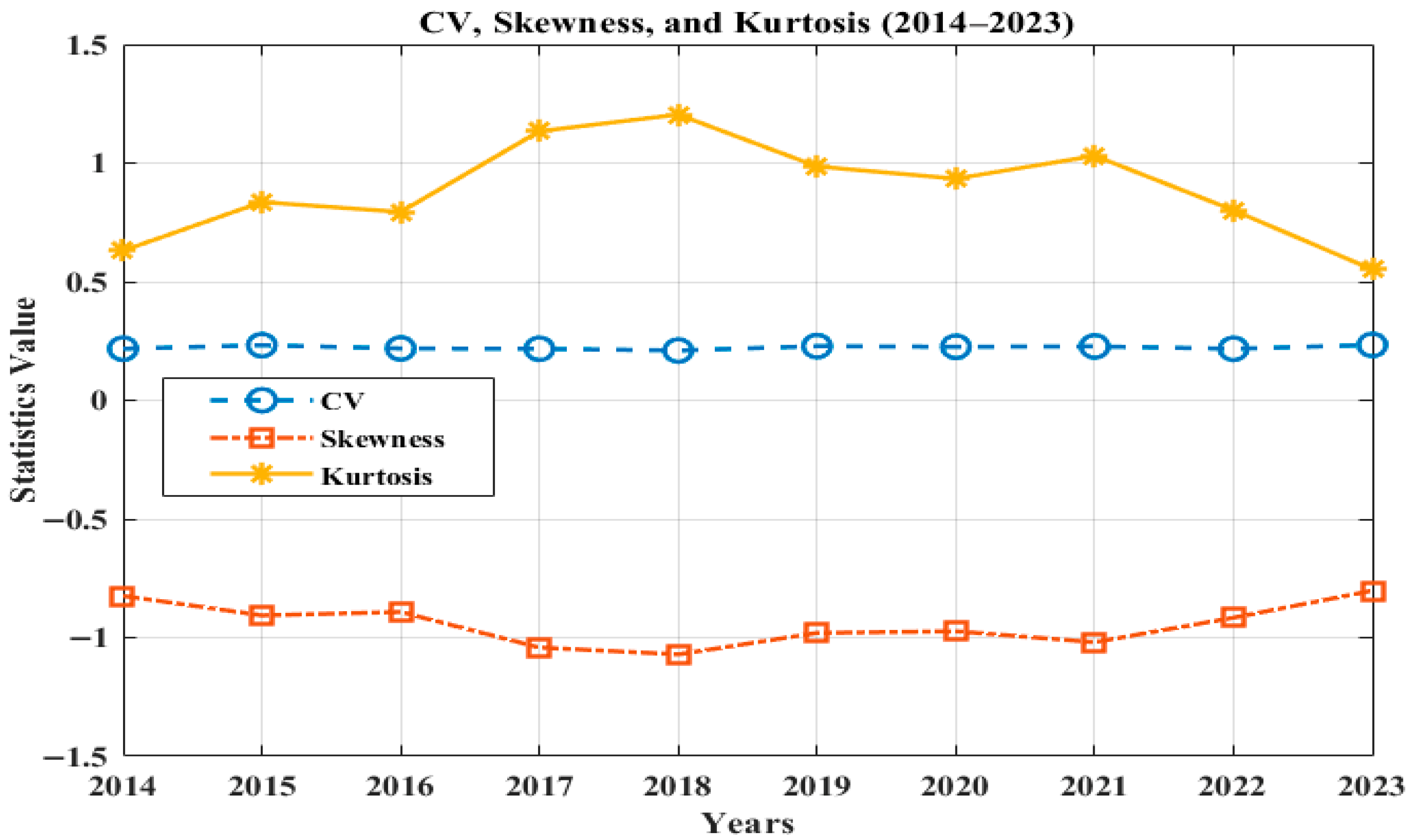
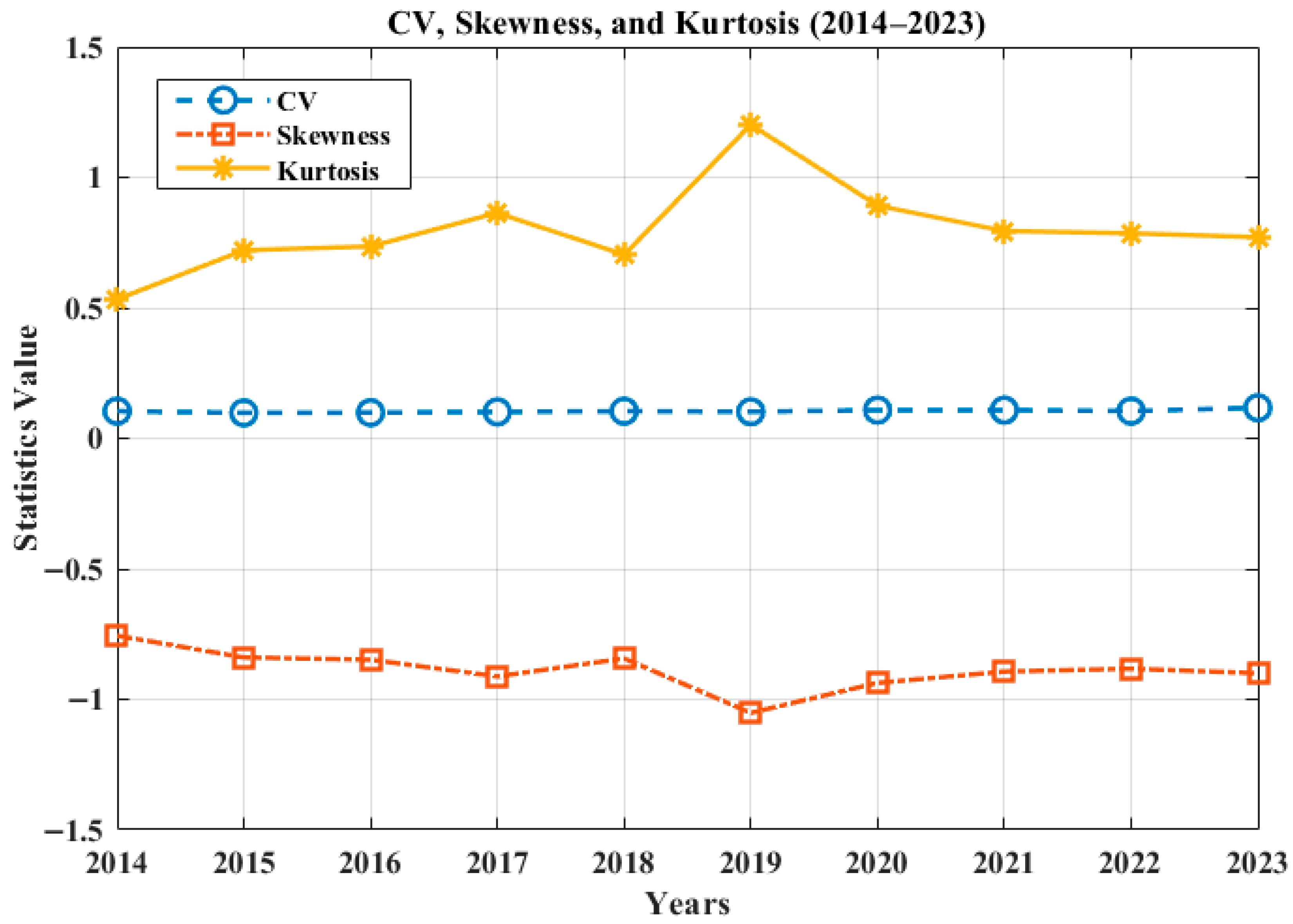
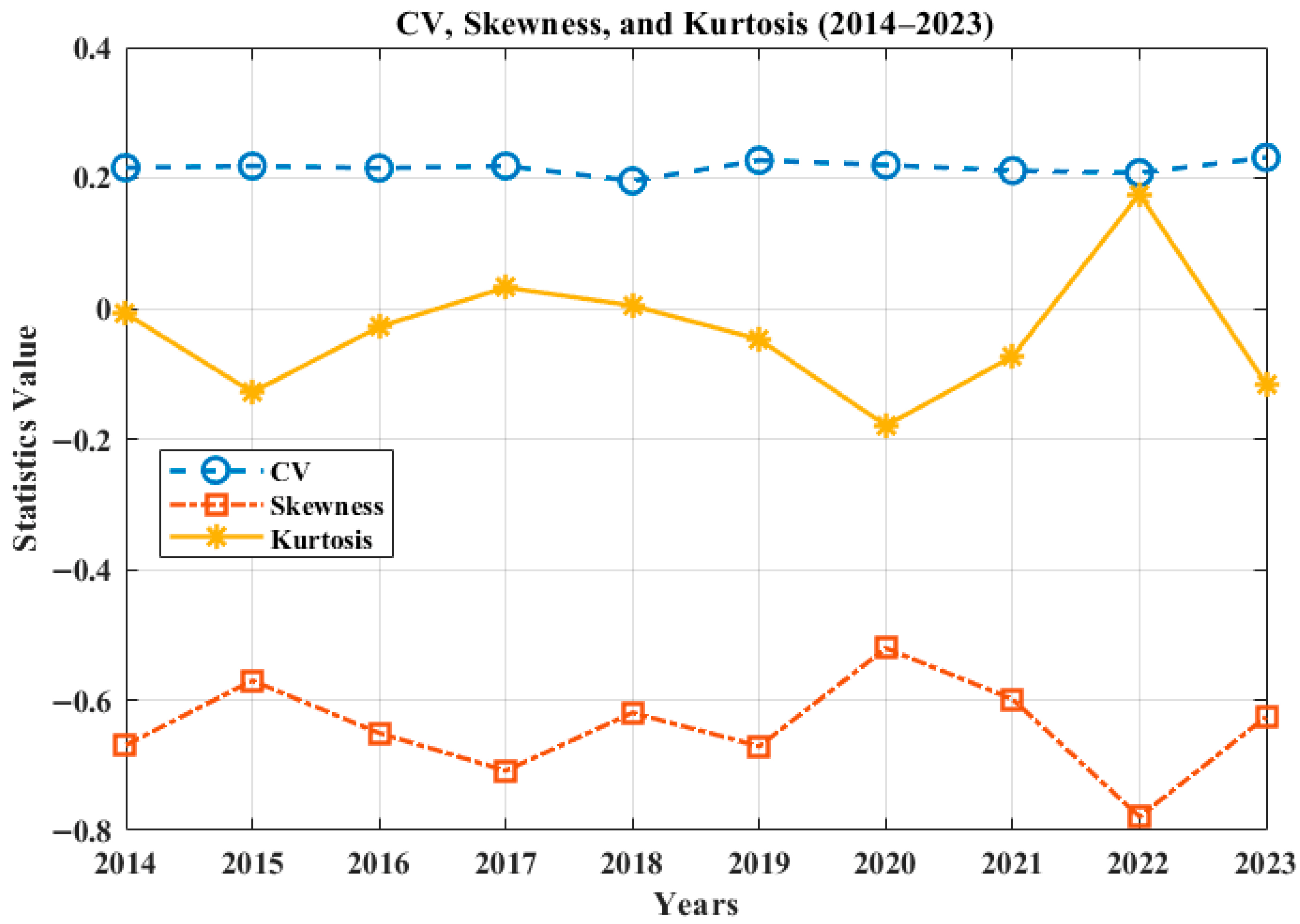
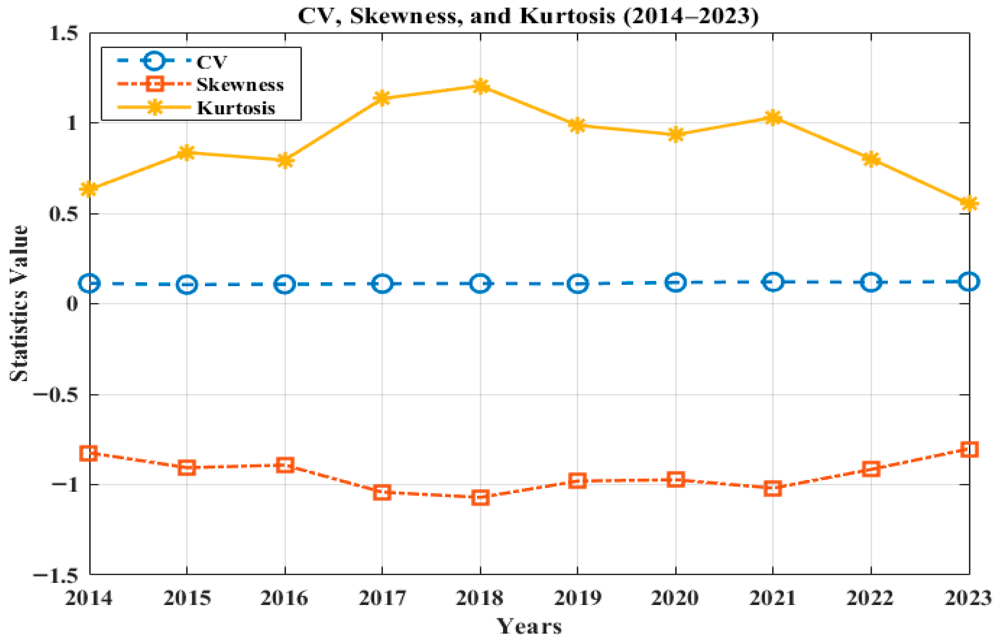
Examining the statistical results from Table 2, Table 3, Table 4, Table 5 and Table 6 shows that the maximum mean value of solar irradiance is found for Site 3: Davanagere with a per-unit value of 0.8666 for the year 2019, whereas the minimum value is 0.6985 for Site 4: Rewa for the year 2020. If the cumulative observation is taken for the complete observational study from 2014 to 2023, the maximum average solar irradiance value of 0.8456 remains the same for Site 3: Davanagere, whereas the minimum average value of 0.7238 is found for Site 2: Jaisalmer. The maximum average variance of 0.0260 is found for Site 2, while the lowest variance value of 0.0078 is found for Site 3. The average values for the whole assessment of mode for the most frequent solar irradiances are 0.8965 and 0.9057 for Site 3 and Site 5, respectively. Graphical representations of other statistics, like the coefficient of variation, skewness, and kurtosis, are shown below in Figure 3, Figure 4, Figure 5, Figure 6 and Figure 7 for each respective site for better understanding.

The variation in coefficient of variation (CV), skewness ($\mathsf{\gamma }$), and kurtosis ($\mathsf{\gamma }$) across sites highlights distinct regional characteristics—higher skewness and CV values indicate greater resource variability, whereas lower kurtosis suggests a more stable energy potential. From Figure 3, Figure 4, Figure 5, Figure 6 and Figure 7, it can be observed that the lowest CV value is 0.0976 for the year 2015 and the lowest average for the whole assessment period is 0.1046 for Site 3. However, Site 2 has a maximum CV of 0.2334 for the year 2023 and a maximum average of 0.2227. From all of the above observations presented tabularly and graphically, it can be observed that Site 3 is a more stable location for solar energy integration than the others due to its higher and more consistent mean solar irradiance with low variation in CV, skewness, and kurtosis.

A solar potential analysis was conducted using the Beta probability distribution function. Although several parameter estimation methods were discussed in Section 1, the Maximum Likelihood method is preferred due to its high accuracy and its ability to handle the large hourly solar irradiance dataset collected over the assessment period. The annually estimated parameters for each site are presented in

Table 7. Parameter estimation using Beta PDF with performance prediction pointers for Kutch.

S. No.	Site 1: Kutch	Parameters of Beta Distribution		Prediction Parameters for Beta Distribution for Solar Potential Analysis
	Year	$\mathit{\alpha }$	$\mathit{\beta }$	RMSE	MAPE	MBE
1.	2014	6.6085	1.9808	0.0391	3.8770	0.0029
2.	2015	7.3045	2.2857	0.0304	4.5188	−0.0048
3.	2016	7.3082	2.1390	0.0387	4.0548	0.0077
4.	2017	5.9698	1.6765	0.0342	4.1680	0.0142
5.	2018	7.2913	2.3101	0.0316	4.2812	−0.0071
6.	2019	6.1809	1.9839	0.0298	4.0019	−0.0095
7.	2020	7.0403	2.3094	0.0369	3.9851	−0.0130
8.	2021	6.7642	1.9905	0.0209	4.4882	0.0061
9.	2022	7.0040	1.9180	0.0298	4.5961	0.0185
10.	2023	6.6999	2.2166	0.0253	4.8584	−0.0151

,

Table 8. Parameter estimation using Beta PDF with performance prediction pointers for Jaisalmer.

S. No.	Site 2: Jaisalmer	Parameters of Beta Distribution		Prediction Parameters for Beta Distribution for Solar Potential Analysis
	Year	$\mathit{\alpha }$	$\mathit{\beta }$	RMSE	MAPE	MBE
1.	2014	4.9496	1.8162	0.0374	5.0165	0.0076
2.	2015	4.5652	1.8187	0.0419	4.8814	−0.0089
3.	2016	5.0018	1.8853	0.0428	4.1954	0.0031
4.	2017	4.2228	1.2991	0.0345	7.1383	0.0407
5.	2018	5.9854	2.5035	0.0382	4.7526	−0.0189
6.	2019	4.7482	1.8881	0.0305	4.4877	−0.0085
7.	2020	4.7114	1.8002	0.0405	4.2352	0.0002
8.	2021	4.6038	1.7486	0.0286	4.9263	0.0007
9.	2022	5.0947	1.9289	0.0386	3.9621	0.0014
10.	2023	4.6779	1.9418	0.0288	5.3593	−0.0173

,

Table 9. Parameter estimation using Beta PDF with performance prediction pointers for Davanagere.

S. No.	Site 3: Davanagere	Parameters of Beta Distribution		Prediction Parameters for Beta Distribution for Solar Potential Analysis
	Year	$\mathit{\alpha }$	$\mathit{\beta }$	RMSE	MAPE	MBE
1.	2014	14.9999	3.1134	0.0326	3.4574	−0.0175
2.	2015	15.2449	2.7580	0.0414	2.5076	0.0012
3.	2016	14.9059	2.6933	0.0355	3.4486	0.0017
4.	2017	13.5302	2.3466	0.0456	2.8643	0.0066
5.	2018	13.8307	2.6202	0.0309	3.6398	−0.0049
6.	2019	11.9178	1.8343	0.0381	3.5074	0.0210
7.	2020	12.0639	2.1491	0.0576	2.9936	0.0036
8.	2021	12.5256	2.3236	0.0463	3.3013	−0.0021
9.	2022	13.3054	2.4292	0.0329	3.9382	0.0000
10.	2023	11.0877	2.1699	0.0382	3.7260	−0.0093

,

Table 10. Parameter estimation using Beta PDF with performance prediction pointers for Rewa.

S. No.	Site 4: Rewa	Parameters of Beta Distribution		Prediction Parameters for Beta Distribution for Solar Potential Analysis
	Year	$\mathit{\alpha }$	$\mathit{\beta }$	RMSE	MAPE	MBE
1.	2014	4.9969	1.8169	0.0376	4.8846	0.0062
2.	2015	5.3504	2.1759	0.0373	4.9868	−0.0162
3.	2016	5.1089	1.8908	0.0380	5.4077	0.0034
4.	2017	4.7137	1.6593	0.0348	5.0131	0.0125
5.	2018	6.2396	2.2682	0.0322	5.4592	0.0063
6.	2019	4.5407	1.6928	0.0295	5.2139	0.0013
7.	2020	5.5364	2.3898	0.0394	5.8513	−0.0277
8.	2021	5.5425	2.1467	0.0277	5.0735	−0.0063
9.	2022	4.8512	1.5514	0.0344	6.7476	0.0305
10.	2023	4.5685	1.8011	0.0289	5.6178	−0.0099

and

Table 11. Parameter estimation using Beta PDF with performance prediction pointers for Anantapur.

S. No.	Site 5: Anantapur	Parameters of Beta Distribution		Prediction Parameters for Beta Distribution for Solar Potential Analysis
	Year	$\mathit{\alpha }$	$\mathit{\beta }$	RMSE	MAPE	MBE
1.	2014	12.5023	2.5651	0.0387	3.5113	−0.0143
2.	2015	12.9166	2.3158	0.0382	3.1011	0.0039
3.	2016	12.6576	2.3408	0.0376	3.6985	0.0003
4.	2017	10.6748	1.7660	0.0448	3.4310	0.0140
5.	2018	10.3140	1.6758	0.0230	4.4505	0.0161
6.	2019	11.3551	1.9697	0.0401	3.0209	0.0081
7.	2020	10.3479	1.9004	0.0483	3.3097	0.0013
8.	2021	9.5942	1.7254	0.0417	3.4805	0.0035
9.	2022	10.7613	2.0908	0.0392	3.9987	−0.0068
10.	2023	11.3128	2.5160	0.0404	4.3774	−0.0260

. Performance prediction indicators were evaluated alongside these parameters to validate the suitability of the selected PDF for potential site assessment. The indicators used include root mean square error (RMSE), mean absolute percentage error (MAPE), and mean bias error (MBE).

Table 6, Table 7, Table 8, Table 9, Table 10 and Table 11 show that the average values of RMSE and MAPE for Sites 1–5 are 0.0317, 0.0362, 0.0399, 0.0340, and 0.0392 and 4.2829%, 4.8955%, 3.3384%, 5.4255%, and 3.6380%, respectively. The average for MBE for all sites is almost negligible, which is a good indicator of data fitting and potential locations. From these indicators, MAPE is still found to be best for Site 3 and the indicators are within the acceptable limits.

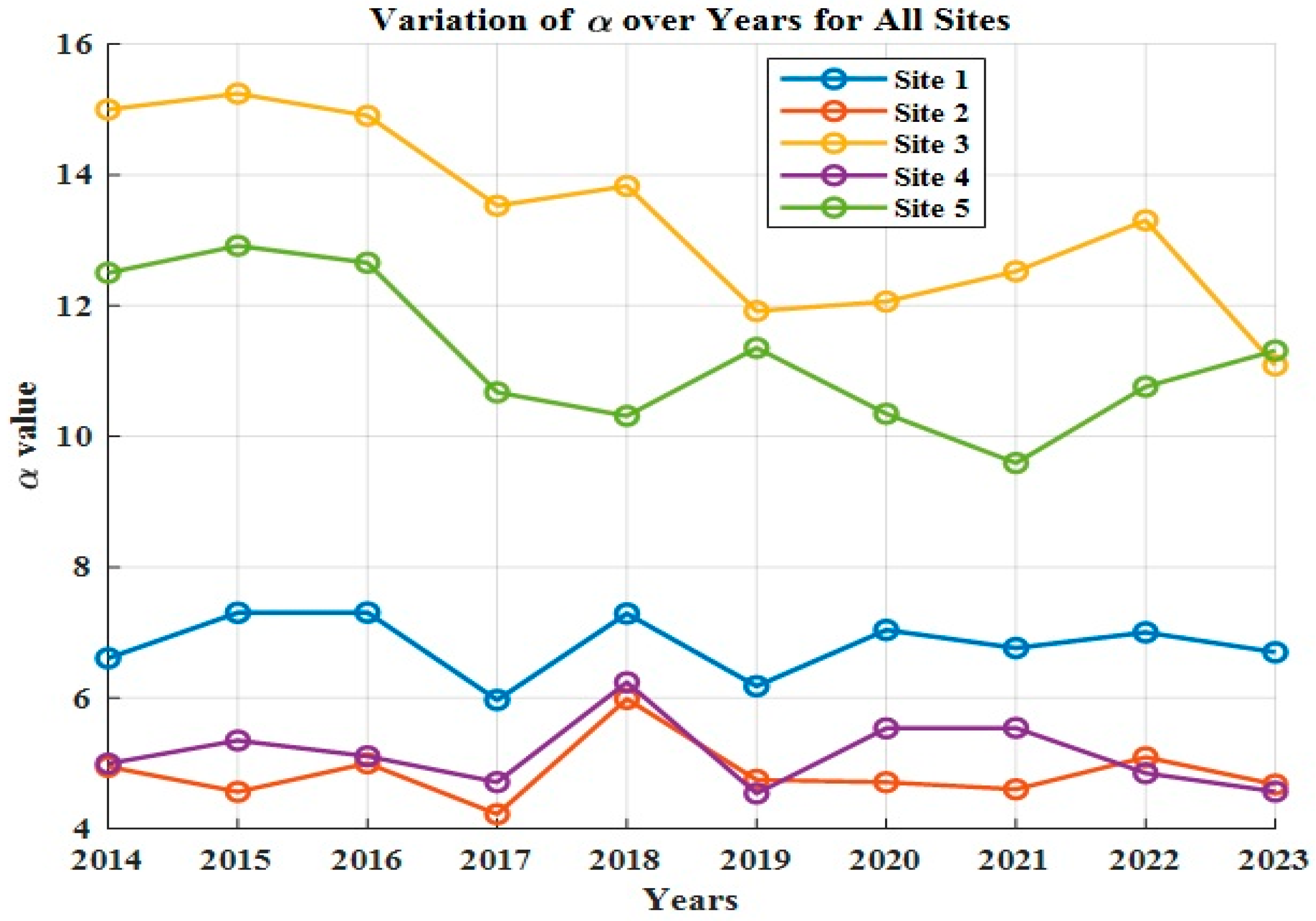
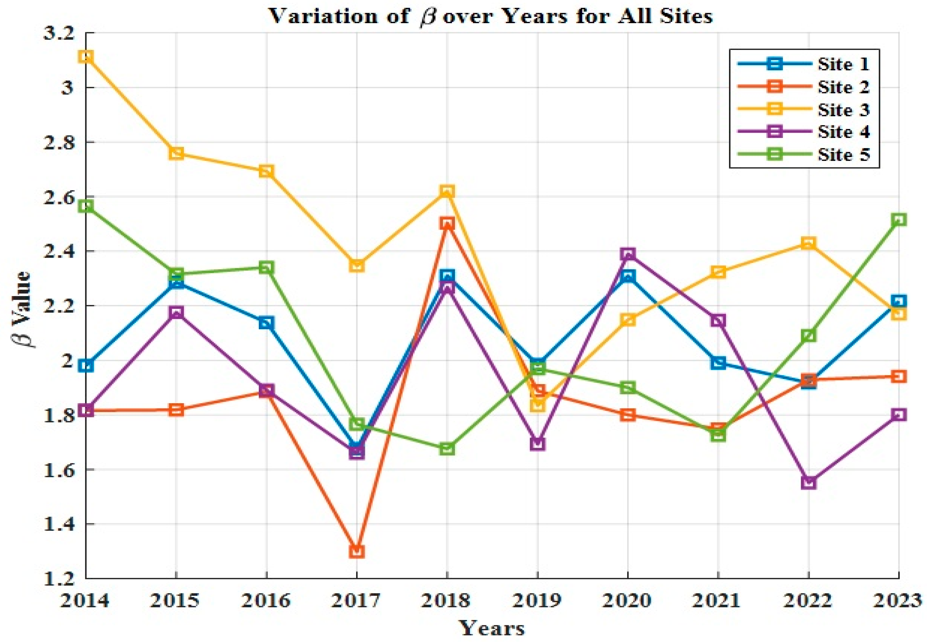
The annual variation in Beta parameters, that is, $\alpha$ and $\beta$, for all locations is shown in Figure 8 and Figure 9, respectively. The Beta distribution curve was drawn for all locations by taking the average value of $\alpha$ and $\beta$ for the whole investigated period from 2014–2023; the findings are collectively represented in Figure 10.

Next, the Kolmogorov–Smirnov fitness test (K-S test) was performed for all potential locations. The K-S statistics along with the p-values are shown in Table 10. For a null hypothesis to be accepted, the K-S value should be less than 0.05 with a p-value greater than 0.01; the sample space for each site is considered as n = 87,600.

In

Table 12. K-S statistics for all potential sites.

Year	Site 1		Site 2		Site 3		Site 4		Site 5
	K-S Statistic	p-Value	K-S Statistic	p-Value	K-S Statistic	p-Value	K-S Statistic	p-Value	K-S Statistic	p-Value
2014	0.042	0.530	0.051	0.292	0.037	0.685	0.028	0.938	0.033	0.808
2015	0.057	0.180	0.030	0.888	0.046	0.402	0.030	0.879	0.050	0.316
2016	0.045	0.442	0.033	0.806	0.031	0.868	0.044	0.467	0.044	0.479
2017	0.051	0.278	0.037	0.675	0.032	0.840	0.045	0.444	0.047	0.390
2018	0.046	0.406	0.050	0.316	0.043	0.509	0.057	0.179	0.066	0.078
2019	0.036	0.725	0.031	0.856	0.042	0.524	0.034	0.787	0.067	0.072
2020	0.036	0.733	0.033	0.812	0.032	0.833	0.046	0.422	0.042	0.519
2021	0.034	0.774	0.041	0.557	0.051	0.285	0.032	0.842	0.044	0.473
2022	0.051	0.284	0.044	0.473	0.048	0.354	0.038	0.642	0.034	0.786
2023	0.051	0.297	0.029	0.919	0.051	0.297	0.032	0.830	0.036	0.720

, the average values of the K-S statistics (also known as D-statistics or D-value) for the complete examination for Sites 1–5 are 0.0499, 0.0379, 0.0413, 0.0385, and 0.0462, respectively, and the p-values are 0.4649, 0.6593, 0.5597, 0.6430, and 0.4642, respectively. The K-S statistics and p-values for all sites are within the permissible range for testing the regularity for fitting, verifying that the assumed null hypothesis can be accepted for this solar potential study.

The outcomes of the Beta distribution parameters and associated performance indicators disclose consistent spatial and chronological patterns across the examined sites. The mean daily irradiance values, ranging from approximately 7.8 to 8.4 kWh·m⁻²·day⁻¹, indicate that all five sites possess strong solar potential suitable for photovoltaic (PV) deployment. Among them, Site 2 exhibits the highest mean irradiance, suggesting greater energy yield potential, while Site 3 demonstrates the lowest coefficient of variation (CV ≈ 0.0078), indicating more stable solar conditions and reduced daily fluctuation.

The negative skewness and low kurtosis observed for Site 3 further confirm a near-symmetric distribution, signifying consistent irradiance availability with minimal extreme events or intermittency. This stability is also reflected in the lowest MAPE (3.34%) and RMSE (0.0399) values, suggesting that the fitted Beta model closely matches the observed irradiance data. In contrast, slightly higher CV and positive skewness values for Sites 1 and 5 point to higher variability caused by transient cloud cover and atmospheric disturbances typical of coastal and semi-arid regions.

Physically, these variations correspond to geographic influences—southern and central inland regions (e.g., Davanagere and Rewa) receive more uniformly distributed solar radiation, whereas western and coastal regions (e.g., Kutch, Jaisalmer) experience seasonal monsoon effects. From a planning perspective, the high mean irradiance of Site 2 makes it ideal for high-yield PV farms, while the exceptional stability of Site 3 is advantageous for hybrid system integration where predictable generation is essential for matching variable wind output.

7.2. Wind Potential Inspection Using Weibull Distribution

The data was collected from a hub height of 50 m in this investigation and can be extrapolated for different hub heights from the ground by means of the power law equation specified below.

$$v_{50}=v_x{\left({\displaystyle \frac{h_{50}}{h_x}}\right)}^{\mathrm{\mu }}$$

where

$\mathrm{\mu }$ = roughness factor and may vary for different geographical locations.

$v \mathrm{a}\mathrm{n}\mathrm{d} h$ are the speed and height at respective locations.

Table 13. Statistics for Weibull distribution for Kutch district, Gujrat.

S. No.	Site 1: Kutch	Mean Statistical Parameters for Weibull Distribution (Annual)
	Year	$${\mathit{\mu }}_{\mathit{w}}$$	$${{\mathit{\sigma }}_{\mathit{w}}}^2$$	$${\mathit{\sigma }}_{\mathit{w}}$$	$${\mathit{C}\mathit{V}}_{\mathit{w}}$$	$${\mathit{M}\mathit{O}}_{\mathit{w}}$$	$${\mathit{\gamma }}_{\mathit{w}}$$	$${\mathit{\kappa }}_{\mathit{w}}$$
1.	2014	6.4210	2.2371	5.0046	0.3484	6.3529	0.0003	0.0010
2.	2015	6.3834	2.1982	4.8319	0.3444	6.3337	0.0003	0.0011
3.	2016	6.3074	2.0760	4.3096	0.3291	6.3207	0.0002	0.0011
4.	2017	6.4150	1.9869	3.9477	0.3097	6.4997	0.0000	0.0011
5.	2018	6.2626	2.1914	4.8024	0.3499	6.1895	0.0004	0.0011
6.	2019	6.1662	2.1353	4.5597	0.3463	6.1099	0.0004	0.0012
7.	2020	5.8849	1.8774	3.5247	0.3190	5.9326	0.0001	0.0015
8.	2021	6.1986	2.2667	5.1380	0.3657	6.0532	0.0005	0.0012
9.	2022	6.2888	2.2735	5.1686	0.3615	6.1616	0.0005	0.0011
10.	2023	6.4433	2.1553	4.6453	0.3345	6.4352	0.0002	0.0010

represents the annual mean statistical parameters for Kutch Gujrat. The parameters include mean values for wind speed $\left({\mu }_w\right)$, variance $\left({{\sigma }_w}^2\right)$, standard deviation $\left({\sigma }_w\right)$, mode $\left({MO}_w\right)$, coefficient of variation $\left({CV}_w\right)$, skewness $\left({\gamma }_{\mathit{w}}\right)$, and kurtosis $\left({\kappa }_w\right)$. Similarly,

Table 14. Statistics for Weibull distribution for Jaisalmer district, Rajasthan.

S. No.	Site 2: Jaisalmer	Mean Statistical Parameters for Weibull Distribution (Annual)
	Year	$${\mathit{\mu }}_{\mathit{w}}$$	$${{\mathit{\sigma }}_{\mathit{w}}}^2$$	$${\mathit{\sigma }}_{\mathit{w}}$$	$${\mathit{C}\mathit{V}}_{\mathit{w}}$$	$${\mathit{M}\mathit{O}}_{\mathit{w}}$$	$${\mathit{\gamma }}_{\mathit{w}}$$	$${\mathit{\kappa }}_{\mathit{w}}$$
1.	2014	5.5030	2.3151	5.3595	0.4207	5.0979	0.0014	0.0019
2.	2015	5.2066	1.7448	3.0444	0.3351	5.1980	0.0004	0.0024
3.	2016	5.1194	2.1044	4.4285	0.4111	4.7926	0.0016	0.0026
4.	2017	5.1459	2.0427	4.1724	0.3970	4.8872	0.0014	0.0025
5.	2018	5.1554	2.3827	5.6774	0.4622	4.5340	0.0023	0.0026
6.	2019	5.1430	2.1591	4.6618	0.4198	4.7690	0.0017	0.0025
7.	2020	5.1849	1.9303	3.7261	0.3723	5.0359	0.0010	0.0024
8.	2021	5.4119	2.1653	4.6886	0.4001	5.1239	0.0012	0.0020
9.	2022	5.4665	2.2946	5.2653	0.4198	5.0693	0.0014	0.0020
10.	2023	5.3921	2.1244	4.5132	0.3940	5.1358	0.0012	0.0021

,

Table 15. Statistics for Weibull distribution for Davanagere district, Karnataka.

S. No.	Site 3: Davanagere	Mean Statistical Parameters for Weibull Distribution (Annual)
	Year	${\mathit{\mu }}_{\mathit{w}}$	${{\mathit{\sigma }}_{\mathit{w}}}^2$	${\mathit{\sigma }}_{\mathit{w}}$	${\mathit{C}\mathit{V}}_{\mathit{w}}$	${\mathit{M}\mathit{O}}_{\mathit{w}}$	${\mathit{\gamma }}_{\mathit{w}}$	${\mathit{\kappa }}_{\mathit{w}}$
1.	2014	5.8844	2.2578	5.0977	0.3837	5.6588	0.0008	0.0014
2.	2015	5.7345	2.4069	5.7932	0.4197	5.3181	0.0012	0.0016
3.	2016	5.7105	2.1793	4.7493	0.3816	5.5017	0.0008	0.0016
4.	2017	5.7520	2.1853	4.7754	0.3799	5.5501	0.0008	0.0016
5.	2018	5.9356	2.4641	6.0719	0.4151	5.5324	0.0011	0.0014
6.	2019	5.9874	2.4232	5.8719	0.4047	5.6424	0.0010	0.0014
7.	2020	5.6672	2.1960	4.8225	0.3875	5.4309	0.0009	0.0017
8.	2021	5.6763	2.1773	4.7407	0.3836	5.4591	0.0009	0.0017
9.	2022	5.5962	2.2493	5.0595	0.4019	5.2886	0.0011	0.0018
10.	2023	5.8732	2.0336	4.1355	0.3462	5.8198	0.0004	0.0015

,

Table 16. Statistics for Weibull distribution for Rewa district, Madhya Pradesh.

S. No.	Site 4: Rewa	Mean Statistical Parameters for Weibull Distribution (Annual)
	Year	${\mathit{\mu }}_{\mathit{w}}$	${{\mathit{\sigma }}_{\mathit{w}}}^2$	${\mathit{\sigma }}_{\mathit{w}}$	${\mathit{C}\mathit{V}}_{\mathit{w}}$	${\mathit{M}\mathit{O}}_{\mathit{w}}$	${\mathit{\gamma }}_{\mathit{w}}$	${\mathit{\kappa }}_{\mathit{w}}$
1.	2014	4.3896	1.6900	2.8560	0.3850	4.2163	0.0019	0.0047
2.	2015	4.2901	1.6138	2.6042	0.3762	4.1531	0.0018	0.0051
3.	2016	4.2968	1.5721	2.4716	0.3659	4.1953	0.0016	0.0051
4.	2017	4.3843	1.5077	2.2732	0.3439	4.3515	0.0009	0.0047
5.	2018	4.4251	1.6864	2.8439	0.3811	4.2653	0.0018	0.0045
6.	2019	4.1534	1.5606	2.4356	0.3757	4.0222	0.0020	0.0058
7.	2020	4.0036	1.4519	2.1080	0.3626	3.9191	0.0018	0.0068
8.	2021	4.2999	1.7462	3.0492	0.4061	4.0463	0.0026	0.0051
9.	2022	4.1074	1.5031	2.2594	0.3660	4.0102	0.0018	0.0061
10.	2023	4.1864	1.5388	2.3680	0.3676	4.0819	0.0017	0.0056

, and

Table 17. Statistics for Weibull distribution for Anantapur district, Andhra Pradesh.

S. No.	Site 5: Anantapur	Mean Statistical Parameters for Weibull Distribution (Annual)
	Year	${\mathit{\mu }}_{\mathit{w}}$	${{\mathit{\sigma }}_{\mathit{w}}}^2$	${\mathit{\sigma }}_{\mathit{w}}$	${\mathit{C}\mathit{V}}_{\mathit{w}}$	${\mathit{M}\mathit{O}}_{\mathit{w}}$	${\mathit{\gamma }}_{\mathit{w}}$	${\mathit{\kappa }}_{\mathit{w}}$
1.	2014	6.3245	2.3217	5.3904	0.3671	6.169	0.0005	0.0011
2.	2015	6.1539	2.2633	5.1224	0.3678	5.9994	0.0006	0.0012
3.	2016	6.0838	2.1202	4.4953	0.3485	6.0189	0.0004	0.0013
4.	2017	5.6979	2.0663	4.2695	0.3626	5.5776	0.0006	0.0016
5.	2018	6.2472	2.4871	6.1859	0.3981	5.9264	0.0008	0.0011
6.	2019	6.2036	2.3408	5.4796	0.3773	5.9994	0.0006	0.0012
7.	2020	5.8507	2.0801	4.3268	0.3555	5.7587	0.0005	0.0015
8.	2021	6.0410	2.0586	4.238	0.3408	6.0086	0.0003	0.0013
9.	2022	5.8613	2.1383	4.5723	0.3648	5.7278	0.0006	0.0015
10.	2023	6.2359	2.0539	4.2187	0.3294	6.2481	0.0002	0.0012

represent the annual mean statistical parameters for Jaisalmer (Rajasthan), Davanagere (Karnataka), Rewa (Madhya Pradesh), and Anantapur (Andhra Pradesh), respectively.

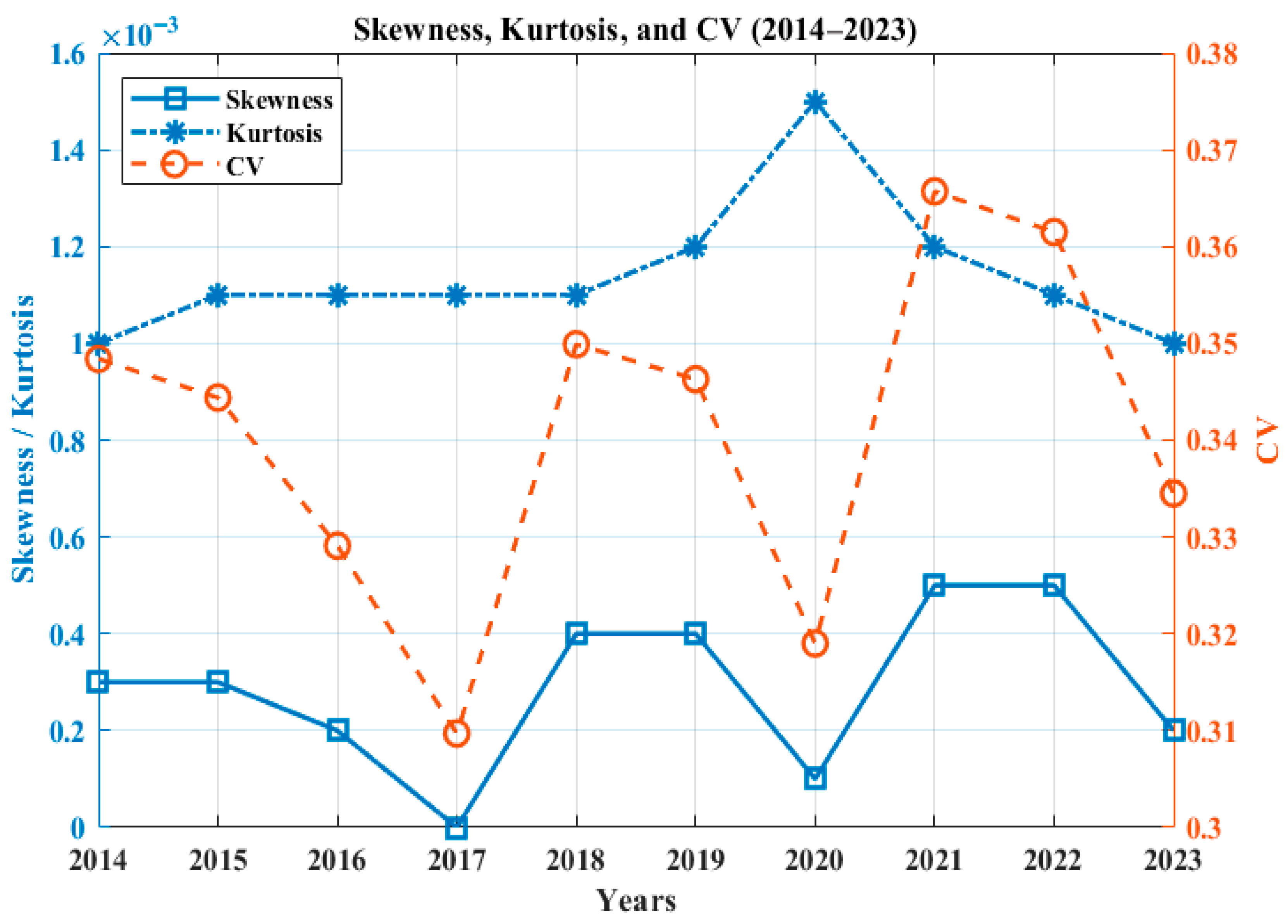
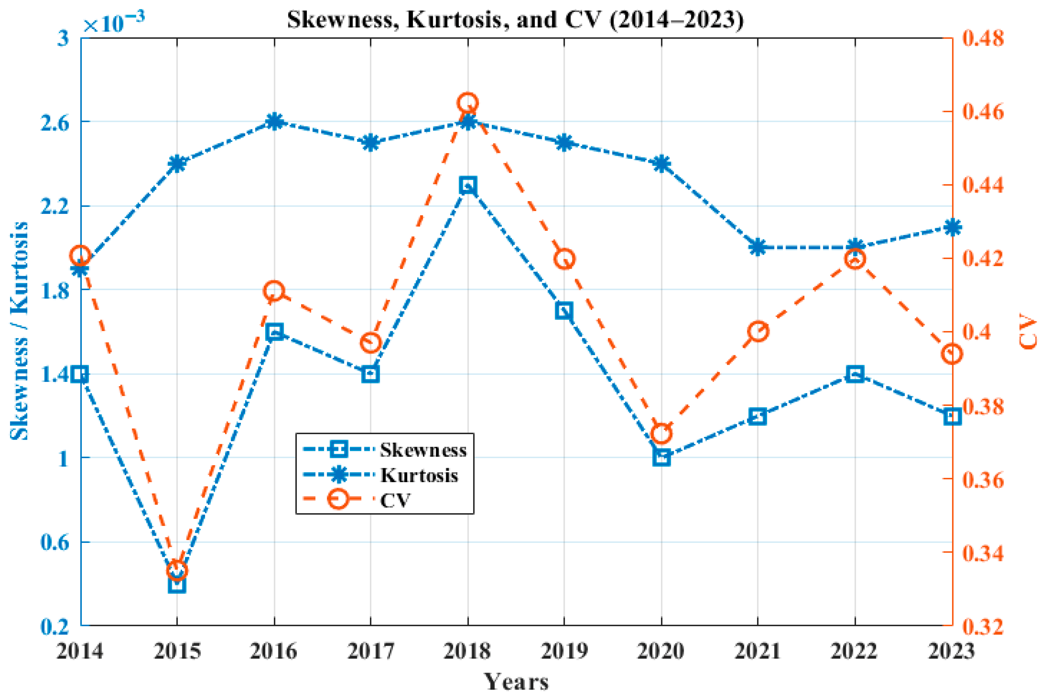
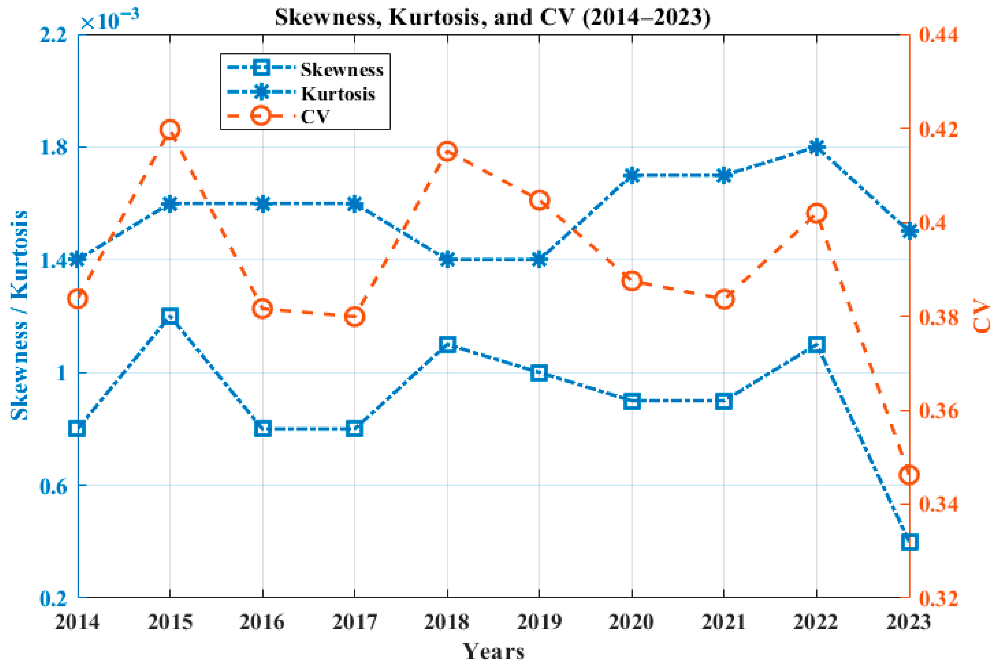
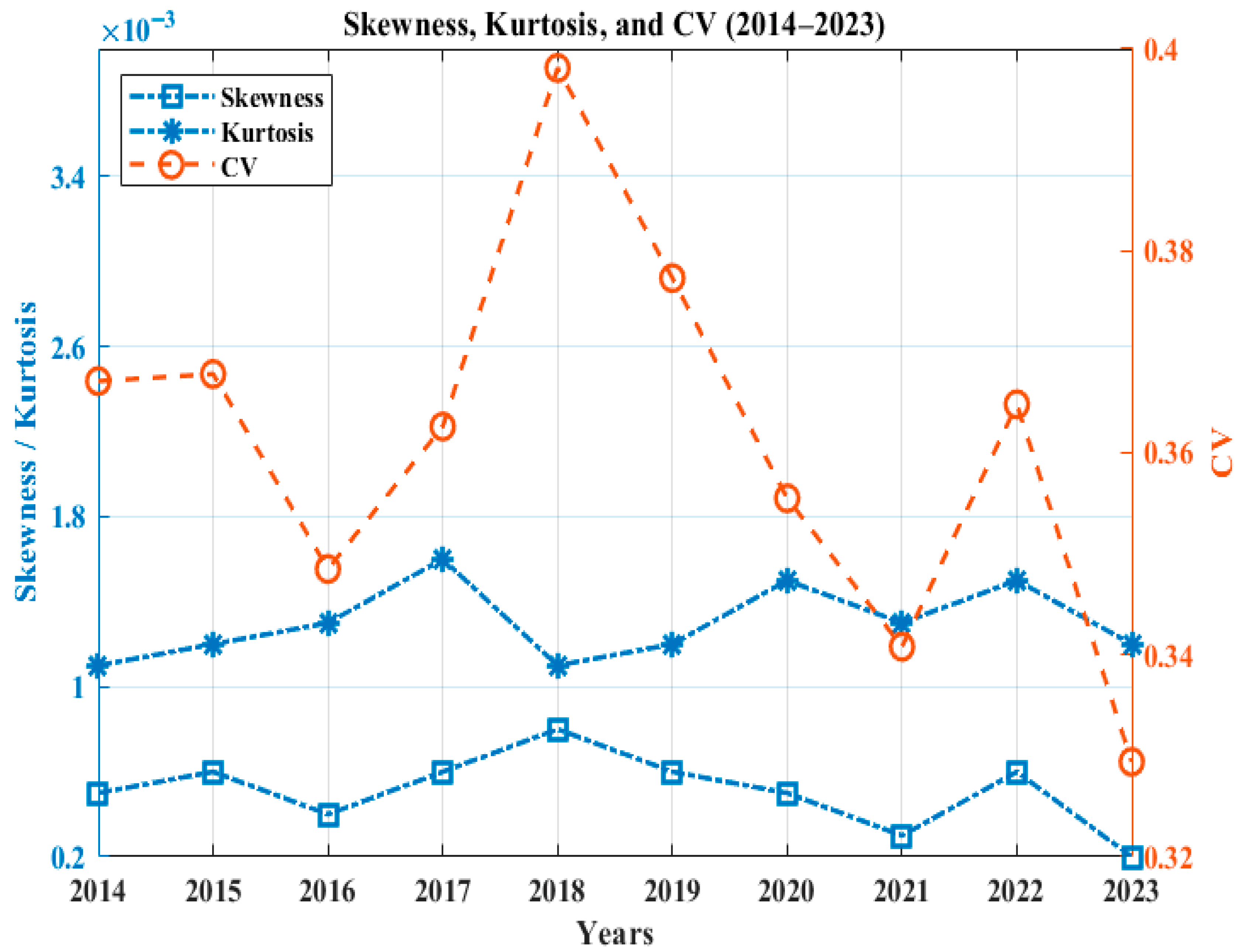
The statistics for the wind potential sites in Table 13, Table 14, Table 15, Table 16 and Table 17 show that the maximum mean wind speed belongs to Site 1 at 6.4433 $\mathrm{m}/\mathrm{s}$ for the year 2023, with highest average value of 6.2271 $\mathrm{m}/\mathrm{s}$ for the whole assessment period. The lowest mean wind speed is found for Site 4 at 4.2537 $\mathrm{m}/\mathrm{s}$. Similarly, the maximum average most frequent wind speed is also found for Site 1 at 6.2389 $\mathrm{m}/\mathrm{s}$, which is represented by mode in this assessment. The maximum and minimum standard deviation and variance are found for Site 3 and Site 4, respectively. The other statistics—coefficient of variation, skewness, and kurtosis—are graphically illustrated in Figure 11, Figure 12, Figure 13, Figure 14 and Figure 15 for each individual site.

The variation in CV, skewness, and kurtosis for all sites are shown in Figure 11, Figure 12, Figure 13, Figure 14 and Figure 15. It can be seen that Site 1 has the average lowest CV of 0.3408 and the lowest skewness and kurtosis values of 0.0003 and 0.0011, respectively. The highest CV is found for Site 2, whereas highest average values for skewness and kurtosis are found for Site 4. The variation in statistics for all locations is within acceptable limits from the perspective of wind potential assessment, indicating that wind turbines can be used here for the generation of electricity. The best statistics are for Site 1, making it the best among the five investigated locations.

The wind potential assessment for the selected locations was conducted using the Weibull probability density function. Parameter estimation was performed using the Maximum Likelihood method due to its precision and ability to capture the intermittent characteristics of wind speed while efficiently handling the large dataset collected over the ten-year study period. The annually computed parameters for all locations are presented in

Table 18. Parameter estimation using Weibull PDF with performance prediction pointers for Kutch.

S. No.	Site 1: Kutch	Parameters of Weibull Distribution		Prediction Parameters for Weibull Distribution for Wind Potential Analysis
	Year	$\mathit{k}$	$\mathit{c}$	RMSE	MAPE	MBE
1.	2014	3.1448	7.1751	0.0190	0.2943	−0.0190
2.	2015	3.1860	7.1286	0.0034	0.0534	0.0034
3.	2016	3.3505	7.0261	0.0074	0.1169	0.0074
4.	2017	3.5846	7.1207	0.0150	0.2347	0.0150
5.	2018	3.1295	6.9997	0.0126	0.2022	0.0126
6.	2019	3.1661	6.8881	0.0038	0.0618	−0.0038
7.	2020	3.4687	6.5437	0.0051	0.0869	−0.0051
8.	2021	2.9796	6.9436	0.0186	0.3017	0.0186
9.	2022	3.0179	7.0406	0.0188	0.2993	0.0188
10.	2023	3.2907	7.1841	0.0133	0.2074	0.0133

,

Table 19. Parameter estimation using Weibull PDF with performance prediction pointers for Jaisalmer.

S. No.	Site 2: Jaisalmer	Parameters of Weibull Distribution		Prediction Parameters for Weibull Distribution for Wind Potential Analysis
	Year	$\mathit{k}$	$\mathit{c}$	RMSE	MAPE	MBE
1.	2014	2.5480	6.1992	0.0130	0.2374	0.0130
2.	2015	3.2840	5.8058	0.0034	0.0648	−0.0034
3.	2016	2.6147	5.7628	0.0194	0.3813	0.0194
4.	2017	2.7188	5.7851	0.0158	0.3085	0.0158
5.	2018	2.2939	5.8195	0.0154	0.3001	0.0154
6.	2019	2.5539	5.7933	0.0070	0.1352	−0.0070
7.	2020	2.9206	5.8130	0.0049	0.0949	0.0049
8.	2021	2.6948	6.0861	0.0219	0.4065	0.0219
9.	2022	2.5543	6.1576	0.0265	0.4866	0.0265
10.	2023	2.7416	6.0602	0.0321	0.5992	0.0321

,

Table 20. Parameter estimation using Weibull PDF with performance prediction pointers for Davanagere.

S. No.	Site 3: Davanagere	Parameters of Weibull Distribution		Prediction Parameters for Weibull Distribution for Wind Potential Analysis
	Year	$\mathit{k}$	$\mathit{c}$	RMSE	MAPE	MBE
1.	2014	2.8239	6.6062	0.0244	0.4166	0.0244
2.	2015	2.5545	6.4595	0.0145	0.2535	0.0145
3.	2016	2.8409	6.4094	0.0105	0.1834	0.0105
4.	2017	2.8553	6.4547	0.0220	0.3834	0.0220
5.	2018	2.5860	6.6837	0.0156	0.2633	0.0156
6.	2019	2.6606	6.7362	0.0275	0.4607	0.0275
7.	2020	2.7929	6.3650	0.0128	0.2258	−0.0128
8.	2021	2.8248	6.3724	0.0062	0.1099	0.0062
9.	2022	2.6811	6.2944	0.0362	0.6506	0.0362
10.	2023	3.1666	6.5608	0.0132	0.2259	0.0132

,

Table 21. Parameter estimation using Weibull PDF with performance prediction pointers for Rewa.

S. No.	Site 4: Rewa	Parameters of Weibull Distribution		Prediction Parameters for Weibull Distribution for Wind Potential Analysis
	Year	$\mathit{k}$	$\mathit{c}$	RMSE	MAPE	MBE
1.	2014	2.8132	4.9288	0.0004	0.0081	−0.0004
2.	2015	2.8871	4.8121	0.0101	0.2363	0.0101
3.	2016	2.9777	4.8133	0.0068	0.1580	0.0068
4.	2017	3.1908	4.8957	0.0058	0.1312	−0.0058
5.	2018	2.8454	4.9664	0.0049	0.1108	−0.0049
6.	2019	2.8906	4.6586	0.0065	0.1569	−0.0065
7.	2020	3.0074	4.4830	0.0037	0.0916	0.0037
8.	2021	2.6504	4.8382	0.0001	0.0026	−0.0001
9.	2022	2.9771	4.6012	0.0026	0.0632	−0.0026
10.	2023	2.9624	4.6907	0.0036	0.0859	−0.0036

and

Table 22. Parameter estimation using Weibull PDF with performance prediction pointers for Anantapur.

S. No.	Site 5: Anantapur	Parameters of Weibull Distribution		Prediction Parameters for Weibull Distribution for Wind Potential Analysis
	Year	$\mathit{k}$	$\mathit{c}$	RMSE	MAPE	MBE
1.	2014	2.9667	7.0859	0.0045	0.0710	0.0045
2.	2015	2.9606	6.8954	0.0039	0.0636	0.0039
3.	2016	3.1438	6.7984	0.0062	0.1011	−0.0062
4.	2017	3.0074	6.3801	0.0079	0.1392	0.0079
5.	2018	2.7098	7.0242	0.0173	0.2774	0.0173
6.	2019	2.8770	6.9594	0.0036	0.0582	0.0036
7.	2020	3.0746	6.5447	0.0093	0.1581	−0.0093
8.	2021	3.2233	6.7424	0.0090	0.1489	−0.0090
9.	2022	2.9875	6.5650	0.0013	0.0228	0.0013
10.	2023	3.3477	6.9467	0.0042	0.0669	−0.0042

. Performance prediction indicators are evaluated alongside these parameters to verify the suitability of the chosen PDF for assessing potential sites. The indicators used include root mean square error (RMSE), mean absolute percentage error (MAPE), and mean bias error (MBE).

Analyzing the performance indicators for all locations shows the lowest average RMSE of 0.0044 for Site 4 at 0.0001 for 2021, with the highest average for Site 3 at 0.0183 with 0.0362 for 2022. The lowest annual average MAPE of 0.1045 was found for Site 4 with a negative MBE, whereas the highest average value of 0.3173 was found for Site 3 at 0.6506 for 2022 and a positive MBE.

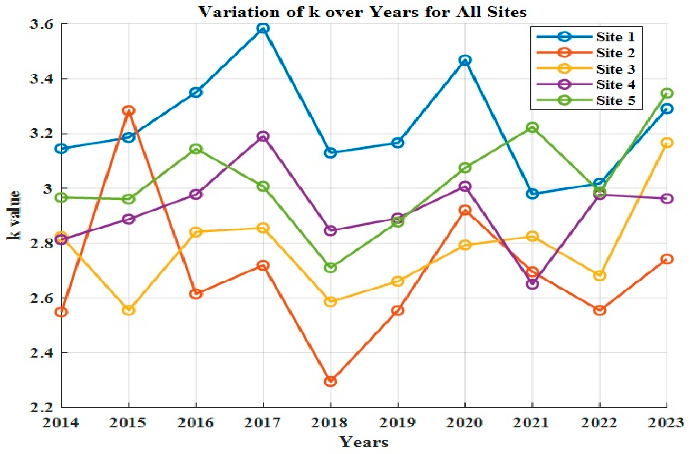
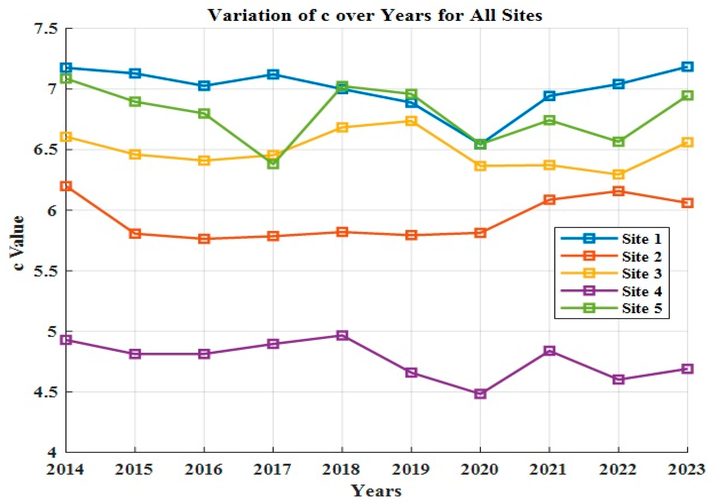
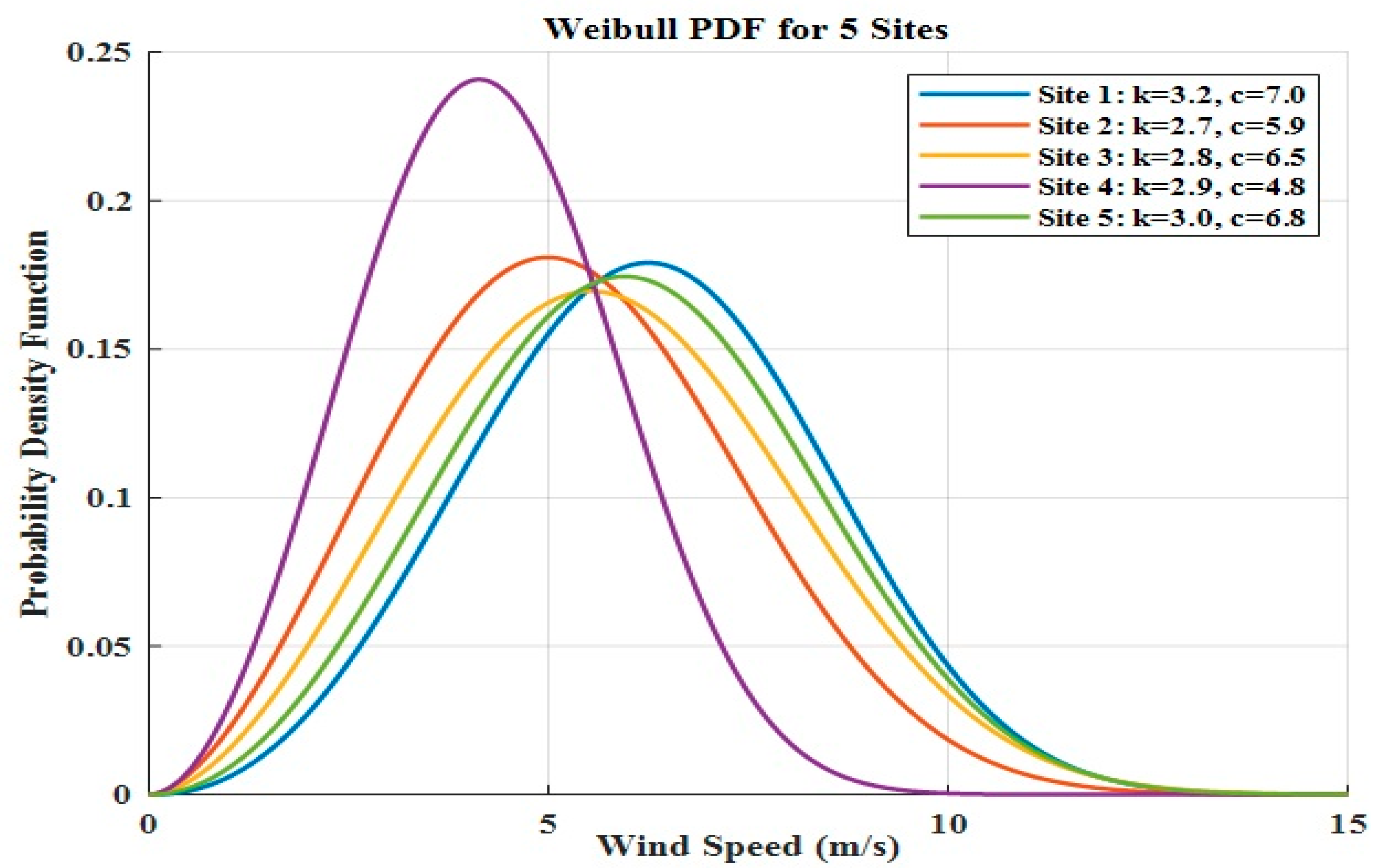
The yearly discrepancies of Weibull parameters, that, is $k$ and $c$, for all sites are shown in Figure 16 and Figure 17, respectively. The Weibull distribution curve was drawn for all locations by taking the mean value of $k$ and $c$ for the entire inspected duration from 2014–2023, and it is jointly represented in Figure 18.

Parameters such as wind power density and maximum energy-carrying wind were analyzed to enhance data accuracy and support the reliable selection of wind turbines for power generation. The average values for both parameters were evaluated for each location annually and are depicted in Table 21. The highest average value of WPD was found for Site 1 at 205.48 $\mathrm{W}/{\mathrm{m}}^2$ with 222.04 $\mathrm{W}/{\mathrm{m}}^2$ for the year 2014, whereas the lowest range of WPD was found for Site 3. Similarly, the highest speeds corresponding to maximum power generation are shown in

Table 23. Supportive parameters for wind potential examination.

Years	$\mathbf{Average} \mathbf{Wind} \mathbf{Power} \mathbf{Density}\left(\mathbf{W}/{\mathbf{m}}^2\right)$$\mathbf{and} \mathbf{Maximum} \mathbf{Energy} \mathbf{Carrying} \mathbf{Wind} \left(\mathbf{m}/\mathbf{s}\right)$ Analysis for Assessment Period (Annual)
	Site 1		Site 2		Site 3		Site 4		Site 5
	$\mathit{W}\mathit{P}\mathit{D}$	${\mathit{V}}_{\mathit{m}\mathit{e}}$	$\mathit{W}\mathit{P}\mathit{D}$	${\mathit{V}}_{\mathit{m}\mathit{e}}$	$\mathit{W}\mathit{P}\mathit{D}$	${\mathit{V}}_{\mathit{m}\mathit{e}}$	$\mathit{W}\mathit{P}\mathit{D}$	${\mathit{V}}_{\mathit{m}\mathit{e}}$	$\mathit{W}\mathit{P}\mathit{D}$	${\mathit{V}}_{\mathit{m}\mathit{e}}$
2014	222.04	7.28	158.83	5.81	181.53	6.47	75.53	4.82	218.96	7.06
2015	216.71	7.26	115.84	5.97	179.41	6.07	69.42	4.75	201.96	6.86
2016	203.99	7.26	125.61	5.47	165.30	6.29	68.52	4.80	188.89	6.90
2017	208.25	7.48	124.31	5.58	168.43	6.34	70.16	4.99	158.90	6.39
2018	206.53	7.09	141.50	5.18	197.26	6.31	76.84	4.87	222.90	6.77
2019	195.96	7.01	129.44	5.44	198.60	6.44	62.95	4.60	210.34	6.86
2020	163.08	6.82	121.73	5.76	163.26	6.20	55.12	4.49	169.98	6.60
2021	205.65	6.93	145.43	5.85	162.91	6.24	73.75	4.62	182.61	6.89
2022	213.23	7.05	155.42	5.78	161.34	6.04	59.86	4.59	173.61	6.56
2023	219.34	7.39	142.26	5.86	169.32	6.67	63.56	4.67	197.21	7.18

.

The Weibull distribution examination illustrates differences in the wind behavior across the five sites. Sites 1 and 5 exhibit the highest average wind power densities (≈206 W/m² and 197 W/m², respectively) and higher maximum energy-carrying wind speeds (≈7 m/s), indicating favorable conditions for wind energy extraction. These results classify both sites under WPD Class 3 (fair resource), suitable for IEC Class II wind turbines. Conversely, Sites 2 and 3 show moderate WPD values (≈135–175 W/m²), which, while lower, still support small- or medium-scale turbine installations. Site 4, with WPD below 70 W/m² and $V_{me}$ ≈ 4.7 m/s, represents a low-wind zone unsuitable for economic wind power generation.

The shape parameter k of the Weibull distribution reflects wind variability, with higher k values indicating more uniform wind speeds—such as those observed at Sites 1 and 5. This stability corresponds to their coastal or near-coastal exposure, where steady monsoon flows and sea-breeze circulation prevail. In contrast, lower k values at inland locations indicate sporadic gusts influenced by local terrain effects. Similarly, the scale parameter c, which is directly associated with the mean wind speed, further reinforces this spatial distinction: higher c values in coastal regions signify stronger and more energetic wind regimes.

From an engineering viewpoint, these findings indicate that Site 1 is best suited for dedicated wind energy generation or hybrid PV–wind configurations, while Site 3, despite lower WPD, offers stable operation that complements solar-rich conditions. The overall pattern illustrates a natural seasonal and spatial complementarity between high solar stability at inland locations and strong wind resources at coastal sites, strengthening the technical feasibility of hybrid system deployment.

When integrating solar and wind analyses, it becomes evident that resource complementarities exist both spatially and temporally. Coastal sites (Sites 1 and 5) show stronger winds during monsoon and nighttime periods, whereas inland sites (Sites 2 and 3) exhibit consistent daytime irradiance. This inverse correlation between solar and wind availability enhances hybrid reliability, reducing storage requirements and improving load-matching capability. Therefore, the combined use of Beta–Weibull probabilistic modeling not only provides accurate resource characterization, but also offers valuable insights for hybrid system configuration and planning across diverse Indian regions.

7.3. Model Validation and Goodness-of-Fit Assessment

To estimate the accuracy of the probabilistic models, the tailored Beta and Weibull distributions were compared with the observed frequency distributions of solar irradiance and wind speed, respectively. Illustrative annual statistical tests for solar (K-S statistics) and wind (WPD and $V_{me}$) verified the strong alignment between the observed and modeled probability density functions. Quantitatively, the low RMSE (<0.05), near-zero MBE, and non-significant K–S test results (p-value > 0.05) confirm that the estimated parameters (α, β) for Beta distribution and (k, c) for Weibull distributions satisfactorily reflect the underlying data. This authentication certifies the trustworthiness of the probabilistic framework for consequent site analysis and energy potential assessment.

7.4. Regional Comparison and Climatic Interpretation

The comparative analysis among the five sites highlights clear regional disparities. Coastal sites such as Kutch and Jaisalmer experience higher wind power density due to their exposure to strong periodic winds and lower terrain roughness. In contrast, inland and elevated sites like Rewa and Davanagere show smoother irradiance patterns and lower variability, attributable to more stable atmospheric conditions. The observed regional differences thus arise from a combination of geographic latitude, proximity to the coast, and monsoonal wind influence. Integrating these characteristics indicates that Site 3 offers superior solar stability, while Sites 1 and 5 exhibit stronger wind regimes—suggesting excellent complementarity for hybrid PV–wind system design.

8. Conclusions

This study was conducted to identify potential hybrid renewable energy sites in India. It was conducted across five different states in India to examine various parameters related to solar and wind power generation. The five potential sites from different regions of India include Kutch (Gujrat), Jaisalmer (Rajasthan), Davanagere (Karnataka), Rewa (Madhya Pradesh), and Anantapur (Andhra Pradesh). For this assessment, hourly point data for solar irradiance and wind speed were collected for a ten-year period from 2014 to 2023. The assessment was accomplished using Beta distribution for solar potential and Weibull distribution for wind potential, respectively. The comprehensive analysis included statistical parameter calculations, the estimation of distribution functions for solar and wind, performance prediction indicators and supportive tests, and investigations of parameters related to solar and wind. Some of the most significant inferences from the above investigations are outlined below.

8.1. Solar Investigation Inferences

• The maximum average values of daily solar irradiance for Site 1 to Site 5 were 8.21, 8.38, 7.85, 8.35, and 7.91 kW-$\mathrm{h}/{\mathrm{m}}^2/\mathrm{d}\mathrm{a}\mathrm{y}$, respectively, for the investigated interval of 2014–2023. Site 2 was found to have the maximum values among all of the studied sites.
• The lowest value of variance was 0.0068 for Site 3 in the year 2015, with the lowest average value of 0.0078 for the same location for solar examinations.
• Site 3 exhibited the lowest value of coefficient of variation along with negative skewness and kurtosis.
• The lowest MAPE of 3.34 was also found for Site 3, with an RMSE of 0.0399 and an almost negligible MBE value.
• The annual variation in Beta parameters was graphically represented for each site along with K-S statistics testing for conformity of data fitting and acceptance of the assumed hypothesis.
• The above examination concludes that Site 3 is the best of the five locations, but all locations can be used for solar integration.

8.2. Wind Investigation Inferences

• The all-time maximum value of wind speed was 18.53 $\mathrm{m}/\mathrm{s}$ for Site 5, with a daily maximum average of 6.28 $\mathrm{m}/\mathrm{s}$ for Site 1.
• The lowest variance and standard deviation were found for Site 4, with all sites exhibiting values in the permissible range.
• The lowest coefficient of variation with positive skewness and kurtosis was found for Site 1.
• Site 4 had the lowest values for MAPE and RMSE with negative MBE.
• The annual variation for Weibull distribution parameters was graphically represented along with supportive parameters for wind site examinations.
• The maximum average value of WPD was 205.48 $\mathrm{W}/{\mathrm{m}}^2$ for Site 1.
• In Table 23, based on the mean WPD and maximum energy-carrying wind speed values, Site 1 falls under Class III as it has strong and stable winds suitable for Class III turbines.
• The wind potential investigation found Site 1 to be the best among the five examined locations with daily maximum average speeds, the lowest CV, the highest energy-carrying wind speeds, and the highest WPD among all sites, although all locations are perfectly suitable for wind power generation.

From the above discussion and interpretation, Site 1 provides stronger wind resources, while Site 3 shows the most stable solar potential. These complementary characteristics suggest that a PV–wind hybrid configuration combining Site 3’s solar stability with Site 1’s wind availability could enhance the overall reliability and energy balance. The uniqueness of this study lies in its use of high temporal resolution and extended period data spanning ten years (2014–2023) with multi-regional and comparative assessments using probabilistic analysis. In contrast to earlier region-specific analyses, this work integrates Beta and Weibull models within a comparative framework and the findings are explicitly interpreted to provide decision-support insights for renewable energy planning at the regional level, aligning with India’s clean energy and sustainability goals under the National Solar and Wind Mission framework. Considering the influence of changing climatic conditions on solar irradiance and wind regimes, the periodic updating and re-evaluation of the dataset are recommended. Continuous measurement and validation will improve the accuracy of the statistical models and ensure the robustness of hybrid system design under future climate scenarios. This solar and wind examination can be further extended for economic and reliability analyses along with storage devices that reduce intermittency of these random nature sources. Further research can include the integration of various other natural resources like biomass or tidal energy generation sources to form a large standalone hybrid power system to meet energy requirements.

References

1. Kumar, A.; Pal, D.; Kar, S.K. An overview of wind energy development and policy initiatives in India. Clean Technol. Environ. Policy 2022, 24, 1337–1358. [Google Scholar] [CrossRef]
2. Luhaniwal, J.; Puppala, H.; Agarwal, S.; Mathur, T. Framework for strategic deployment of hybrid offshore solar and wind power plants: A case study of India. J. Clean. Prod. 2024, 479, 144009. [Google Scholar] [CrossRef]
3. Renewable Energy Statistics, Government of India, Ministry of New and Renewable Energy (MNRE) 2023–2024. Available online: https://mnre.gov.in/en/renewable-energy-statistics (accessed on 15 April 2025).
4. Sumair, M.; Aized, T.; Gardezi, S.A.R.; ur Rehman, S.U.; Rehman, S.M.S. Wind potential estimation and proposed energy production in Southern Punjab using Weibull probability density function and surface measured data. Energy Explor. Exploit. 2021, 39, 2150–2168. [Google Scholar] [CrossRef]
5. Wahbah, M. Unbiased cross-validation kernel density estimation for wind and PV probabilistic modelling. Energy Convers. Manag. 2022, 266, 115811. [Google Scholar] [CrossRef]
6. Liu, L.; Zhai, R.; Hu, Y. Performance evaluation of wind-solar-hydrogen system for renewable energy generation and green hydrogen generation and storage: Energy, exergy, economic, and enviroeconomic. Energy 2023, 276, 127386. [Google Scholar] [CrossRef]
7. Boulahia, M.; Djiar, K.A.; Amado, M.P. Combined Engineering—Statistical Method for Assessing Solar Photovoltaic Potential on Residential Rooftops: Case of Laghouat in Central Southern Algeria. Energies 2021, 14, 1626. [Google Scholar] [CrossRef]
8. Chikh, M.; Haddadi, M.; Mahrane, A.; Malek, A. Assessment of the diffuse component of the global horizontal solar radiation for different solar altitude ranges. Case study: Oran (Algeria). IET Renew. Power Gener. 2019, 13, 640–649. [Google Scholar] [CrossRef]
9. Abdulkarim, A.; Abdelkader, S.M.; Morrow, D.J. Statistical Analyses of Wind and Solar Energy Resources for the Development of Hybrid Microgrid; Springer: Cham, Switzerland, 2015; pp. 9–14. [Google Scholar]
10. Avila, C.; Forero, S.; Bueno-Lopez, M. Methods for the Characterization of the Variability of Solar and Wind Resource; Springer: Cham, Switzerland, 2019; pp. 224–233. [Google Scholar]
11. Manusov, V.; Khaldarov, S.H. Power Distribution Laws Modelling of Wind Power and Solar Stations. Probl. Reg. Energetics 2020, 47, 81–91. [Google Scholar]
12. Didane, D.H.; Manshoor, B. Assessment of Wind Power Potentials in Chittagong, Bangladesh Using Weibull Distribution Function. J. Adv. Res. Fluid Mech. Therm. Sci. 2023, 105, 154–165. [Google Scholar] [CrossRef]
13. Wais, P. A review of Weibull functions in wind sector. Renew. Sustain. Energy Rev. 2017, 70, 1099–1107. [Google Scholar] [CrossRef]
14. Yadav, A.; Malik, H.; Yadav, V.; Alotaibi, M.A.; García Márquez, F.P.; Afthanorhan, A. Comparative Analysis of Weibull Parameters Estimation for Wind Power Potential Assessment. Results Eng. 2024, 23, 102300. [Google Scholar] [CrossRef]
15. Youcef, F.; Ettoumi, A.; Mefti, A.; Adane, M.Y. Bouroubi Statistical analysis of solar measurements in Algeria using beta distributions. Renew. Energy 2002, 26, 47–67, ISSN 0960-1481. [Google Scholar] [CrossRef]
16. Kolhe, M. Techno-Economic Optimum Sizing of a Stand-Alone Solar Photovoltaic System. IEEE Trans. Energy Convers. 2009, 24, 511–519. [Google Scholar] [CrossRef]
17. Ihaddadene, R.; Ihaddadene, N. Modelling of monthly global solar radiation in M’sila region (Algeria). In Proceedings of the 2016 7th International Renewable Energy Congress (IREC), Hammamet, Tunisia, 22–24 March 2016; pp. 1–6. [Google Scholar]
18. Kolhe, M.; Joshi, J.C.; Kothari, D.P. Performance analysis of a directly coupled photovoltaic water-pumping system. IEEE Trans. Energy Convers. 2004, 19, 613–618. [Google Scholar] [CrossRef]
19. Arun Rathore, N.P. Patidar. Reliability assessment using probabilistic modelling of pumped storage hydro plant with PV-Wind based standalone microgrid. Int. J. Electr. Power Energy Syst. 2019, 106, 17–32. [Google Scholar] [CrossRef]
20. Rathore, A.; Patidar, N.P. Optimal sizing and allocation of renewable based distribution generation with gravity energy storage considering stochastic nature using particle swarm optimization in radial distribution network. J. Energy Storage 2021, 35, 102282. [Google Scholar] [CrossRef]
21. Khatib, T.; Mohamed, A.; Sopian, K. Review of solar energy modelling techniques using probability distributions. Renew. Sustain. Energy Rev. 2012, 16, 2864–2969. [Google Scholar] [CrossRef]
22. Carta, J.A.; Ramírez, P.; Velázquez, S. A review of wind speed probability distributions used in wind energy analysis. Renew. Sustain. Energy Rev. 2009, 13, 933–955. [Google Scholar] [CrossRef]
23. Patel, S.; Patidar, N.P. Optimal Forecasting and credibility-based Assessment of a standalone system to comprehend Biomass/Wind/Solar in contextual of rural India. Sci. Technol. Energy Transit. 2025, 80, 31. [Google Scholar] [CrossRef]
24. IRENA. Renewable Energy Statistics 2024; International Renewable Energy Agency: Abu Dhabi, United Arab Emirates, 2024; Available online: https://www.irena.org/ (accessed on 15 April 2025).
25. Rahman, M.; Amin, M.I. Note on Parameter Estimation in Beta Distribution. Far East J. Theor. Stat. 2024, 68, 255–262. [Google Scholar] [CrossRef]
26. Ali, H.; Akanihu, C.N.; Felix, J. Investigating the parameters of the beta distribution. World J. Adv. Res. Rev. 2023, 19, 815–830. [Google Scholar] [CrossRef]
27. Ben, U.C.; Akpan, A.E.; Mbonu, C.C.; Ufuafuonye, C.H. Integrated technical analysis of wind speed data for wind energy potential assessment in parts of southern and central Nigeria. Clean. Eng. Technol. 2021, 2, 100049. [Google Scholar] [CrossRef]
28. Shaban, A.H.; Resen, A.K.; Bassil, N. Weibull parameters evaluation by different methods for windmills farms. Energy Rep. 2020, 6, 188–199. [Google Scholar] [CrossRef]
29. Wahbah, M.; EL-Fouly, T.H.M.; Zahawi, B.; Feng, S. Hybrid Beta-KDE Model for Solar Irradiance Probability Density Estimation. IEEE Trans. Sustain. Energy 2020, 11, 1110–1113. [Google Scholar] [CrossRef]
30. Wahbah, M.; Zahawi, B.; El-Fouly, T.H.M. Solar Probability Density Estimation Using Adaptive Parametric/Nonparametric Hybrid Model. IEEE Access 2024, 12, 195412–195421. [Google Scholar] [CrossRef]
Figure 3. Coefficient of variation ( C V B ) skewness γ B , and kurtosis κ B for Site 1.
Energies 18 06076 g003
Figure 4. Coefficient of variation ( C V B ) skewness γ B , and kurtosis κ B for Site 2.
Energies 18 06076 g004
Figure 5. Coefficient of variation ( C V B ) skewness γ B , and kurtosis κ B for Site 3.
Energies 18 06076 g005
Figure 6. Coefficient of variation ( C V B ) skewness γ B , and kurtosis κ B for Site 4.
Energies 18 06076 g006
Figure 7. Coefficient of variation ( C V B ) skewness γ B , and kurtosis κ B for Site 5.
Energies 18 06076 g007
Figure 8. Annual variation of α for all sites.
Energies 18 06076 g008
Figure 9. Annual variation of β for all sites.
Energies 18 06076 g009
Figure 10. Beta PDF for all sites.
Energies 18 06076 g010
Figure 11. Skewness ( γ w ) , kurtosis ( κ w ) , and coefficient of variation ( C V w ) for Site 1.
Energies 18 06076 g011
Figure 12. Skewness ( γ w ) , kurtosis ( κ w ) , and coefficient of variation ( C V w ) for Site 2.
Energies 18 06076 g012
Figure 13. Skewness ( γ w ) , kurtosis ( κ w ) , and coefficient of variation ( C V w ) for Site 3.
Energies 18 06076 g013
Figure 14. Skewness ( γ w ) , kurtosis ( κ w ) , and coefficient of variation ( C V w ) for Site 4.
Energies 18 06076 g014
Figure 15. Skewness ( γ w ) , kurtosis ( κ w ) , and coefficient of variation ( C V w ) for Site 5.
Energies 18 06076 g015
Figure 16. Annual variation of k for all sites.
Energies 18 06076 g016
Figure 17. Annual variation of c for all sites.
Energies 18 06076 g017
Figure 18. Weibull PDF for all sites.
Energies 18 06076 g018