Abstract
Lightning-induced backflashovers pose significant risks to high-voltage transmission systems, particularly in high lightning activity regions. Conventional backflashover rate (BFR) estimation methods rely on simplified empirical formulas that lack accuracy in complex scenarios. This paper presents a comprehensive simulation framework integrating (i) a Simulation-Based Leader Progression Model (SB-LPM) implemented in COMSOL Multiphysics–MATLAB to evaluate lightning attachment through detailed electrostatic field analysis and streamer-leader dynamics, (ii) ATP-EMTP electromagnetic transient simulations incorporating multi-component Heidler function current waveforms, calibrated to regional lightning measurements, and (iii) a Monte Carlo analysis for statistical assessment of backflashover susceptibility. Applied to a representative 138 kV transmission line in Minas Gerais, Brazil, the framework shows that BFR results are highly sensitive to tower-footing impedance and attachment model selection. The SB-LPM yields systematically different predictions compared to traditional electrogeometric models, yielding approximately 10% lower BFR estimates at 20 Ω grounding impedance relative to the widely used Eriksson model. The framework enables comprehensive lightning performance assessment by incorporating geometry-sensitive attachment modeling, realistic current waveform synthesis, and detailed system transient response, providing valuable insights for transmission line insulation coordination studies.
1. Introduction
Lightning-induced failures are a leading cause of unplanned outages in power transmission systems, accounting for an estimated 20–40% of reliability incidents in regions with moderate to high lightning densities. Factors such as elevated shielded towers, moderate insulation strength, and complex surge propagation dynamics make high-voltage lines particularly susceptible to lightning-induced backflashovers [1,2]. This phenomenon occurs when lightning strikes a tower or its shield wire, leading to transient overvoltages that exceed the insulation withstand threshold and cause phase-to-ground arcs [1]. Consequently, accurate quantification of backflashover risk is essential for insulation coordination, reliability assessment, and the design of effective lightning protection measures in transmission systems.
Predicting transmission line backflashover performance presents a multifaceted challenge: it requires modeling the attachment process under realistic electric field conditions, representing the injected lightning current waveform and its interaction with the line, simulating electromagnetic transients through detailed system models, and evaluating insulation breakdown using appropriate physical or statistical criteria. These components must be integrated within a probabilistic framework to capture the variability in lightning parameters, grounding conditions, and insulation strength that governs backflashover risk in real-world environments.
Conventional methods for estimating the backflashover rate (BFR) rely on simplified lightning exposure calculations based on empirical formulas, which express the attractive radius or striking distance as a function of return stroke peak current and geometrical configuration [2,3]. However, these approaches presuppose deterministic attachment behavior and do not resolve the dynamics of downward leader propagation or upward connecting leaders [4]. Moreover, they decouple the attachment process from the system’s transient response, relying on idealized current waveforms and neglecting the influence of waveform steepness, injection location, and frequency-dependent system impedance [5,6]. Insulation breakdown is typically assessed using fixed thresholds, omitting environmental dependencies and statistical dispersion [7,8]. These simplifications lead to BFR estimates that lack fidelity and the uncertainty quantification required for accurate performance assessment—particularly in high-lightning-density regions, where stochastic variations in strike severity and system configuration strongly influence backflashover risk [9,10,11].
To overcome the limitations of empirical stroke incidence approaches, Leader Progression Models (LPMs) have been developed that explicitly simulate the development of downward stepped leaders and upward connecting leaders. Notable examples include the engineering-oriented model by Rizk [12,13], the physics-based approach by Dellera and Garbagnati [14,15], and the semi-empirical formulation by Eriksson [3]. A significant advancement in this field is the Self-Consistent Leader Inception and Propagation Model (SLIM), introduced by Becerra and Cooray [16], which self-consistently computes key physical parameters—such as charge per unit length, potential gradient, channel radius, injected current, and propagation velocity—throughout the leader propagation process.
SLIM, along with conceptually aligned models developed by Arevalo and Cooray [17], leverages finite element electromagnetic simulations to dynamically determine streamer and upward leader parameters under varying electric field conditions imposed by the descending stepped leader. This approach addresses key limitations associated with fixed-parameter models, which may not adequately capture the dynamic nature of natural lightning. Cooray and collaborators have applied these models to evaluate the efficiency of lightning conductors [16,17], simulate lightning attachment to complex structures [16], and transmission line towers [17], demonstrating that field-based models can effectively predict attachment conditions. Furthermore, their findings show that such simulations can yield substantially different attachment predictions compared to classical electrogeometric models (EGMs), particularly regarding structure height and shielding design [18].
Building upon these advances, the present study introduces a Simulation-Based Leader Progression Model (SB-LPM), which incorporates detailed electrostatic simulations and explicit streamer-leader dynamics into a probabilistic backflashover performance assessment framework. The method integrates COMSOL–MATLAB simulations of lightning attachment, ATP–EMTP transient electromagnetic analysis, region-specific double-peak return stroke current representation, and a Monte Carlo approach for stochastic flashover risk quantification.
Recent field experience indicates that transmission voltage levels in the 69–230 kV range frequently exhibit high rates of lightning-induced outages [1]. This stems from a combination of moderate insulation strength and frequent exposure to direct lightning strikes. In contrast, higher-voltage systems usually employ longer insulation strings and benefit from enhanced shielding, making them less susceptible to direct strikes, while lower-voltage lines are more vulnerable to induced overvoltages—a phenomenon outside the present scope.
The proposed framework is demonstrated through an extensive case study of a 138 kV transmission line in Minas Gerais, Brazil. This selection serves both a practical necessity, given the global prevalence and vulnerability of such systems, and a methodological purpose, providing a challenging test case to validate the predictive distinctiveness of physics-based attachment models relative to established electrogeometric methods.
Moreover, the present framework incorporates a detailed 3D model of the tower geometry, representing an advance over commonly used simplified representations. This enables a more realistic and geometry-sensitive assessment of lightning attachment even at these voltage levels.
By providing physically informed, geometry-sensitive, and statistically consistent BFR predictions, this methodology offers practical insights for insulation coordination, risk assessment, and transmission line design optimization.
The structure of this paper is as follows: Section 2 details the integrated simulation framework, covering lightning attachment modeling, transient analysis, and the Monte Carlo approach for backflashover probability. Section 3 presents the comprehensive simulation results derived from the case study. Section 4 analyzes these results and discusses their broader implications. Section 5 summarizes key findings and suggests directions for future research.
2. Methodology
2.1. Probabilistic Framework for Backflashover Rate Estimation
The backflashover rate (BFR) quantifies the expected number of lightning-induced backflashovers per year. In this work, the BFR is represented through a two-stage probabilistic model:
- Interception Stage: A lightning stroke is intercepted by the shield wire;
- Flashover Stage: Following interception, the resultant overvoltage may cause an insulation flashover.
Within this framework, the BFR (flashovers per year) is expressed as [1]:
Equation (1) expresses the backflashover rate as a two-stage probabilistic formulation, combining the flash collection rate with the conditional probability of flashover for each intercepted stroke, where
- PBFO(I,τ(I),φ) is the conditional probability that a lightning stroke of peak current I and correlated front time τ = g(I), intercepted by the shield wire, leads to flashover given the system phase angle φ at impact.
- Ksf is the span factor, which represents the fraction of lightning strokes that occur near or at tower tops, making them more likely to generate significant overvoltages [11].
- NS is the flash collection rate (FCR, flashes/year) [11,19]:
Here:
- Psw(I, x) is the probability that a descending leader with current I and lateral displacement x is intercepted by the shield wire;
- Ng is the regional ground flash density (GFD, flashes/km2/year);
- w is the transverse width of the analyzed strike zone (m);
- L is the line length (km).
The probability density functions fI(I), fx(x) and fφ(φ) describe the statistical distribution of the lightning currents, lateral offsets, and voltage phase angles, respectively. Lighting current typically follow a log-normal distribution [1,2]:
where μln and σln are the mean and standard deviations of ln(I).
The interception probability Psw (I, x) depends on the lightning attachment model used, detailed in Section 2.2. The flashover probability PBFO(I,τ(I),φ) is evaluated via transient simulations in ATP-EMTP, comparing induced overvoltages with insulation withstand limits (Section 2.3).
2.2. Lightning Stroke Attachment Modeling
The FCR calculation depends on the exposure width of the transmission line structure and the interception probability for lightning strokes [2]. The interception probability is dictated by the attachment model, which determines if a stroke with a given lateral offset and prospective current will strike the shield wire, phase conductor, or ground.
Three modeling approaches are considered in this work:
- Eriksson’s empirical attractive radius formulation (fixed radius) [3];
- Electrogeometric striking distance models (EGMs) [2,20,21,22,23,24,25];
- Simulation-based Leader Progression Model (SB-LPM, original implementation in this work).
2.2.1. Eriksson’s Empirical Attractive Radius
The Leader Progression Model (LPM) explicitly describes the inception and propagation of upward connecting leaders, with the attractive radius R(I, h) defining the lateral distance within which a tower of height h intercepts a stroke of current I. A general formulation is [11,23]:
where ξ, E, and F are model-specific constants. For a double-shield wire configuration, the stroke incidence, Ns, in flashes per100 km-year can be expressed as [11,19]:
where Sg is the horizontal separation between shield wires.
Eriksson [3] proposed a simplified expression for the average attractive radius based on field data from transmission lines:
which can be substituted into Equation (5) to estimate the flash collection rate deterministically. This widely used empirical formulation corresponds to a representative return-stroke current (commonly 30 kA) and is adopted in many lightning performance assessments as a practical reference baseline (see, e.g., [1,2]):
2.2.2. Electrogeometric Models (EGMs)
Electrogeometric models (EGMs) describe lightning attachment in terms of the striking distance between the descending stepped leader and the structure, expressed as a function of the return-stroke peak current. Different parameterizations exist (e.g., Armstrong–Whitehead [20], Brown–Whitehead [21], Love [22], Anderson [23], IEEE formulations [2,24], Darveniza [25]), and they are widely used in shielding and lightning performance studies.
In this work, EGMs are included as benchmark formulations for comparison with the empirical and simulation-based approaches. The detailed equations, parameter sets, and flash collection rate derivations are provided in Appendix A (Table A1).
2.2.3. Simulation-Based Leader Progression Model (SB-LPM)
Lightning attachment to transmission towers significantly impacts the backflashover rate in high-voltage transmission lines. To accurately model this phenomenon, this study introduces a simulation-based Leader Progression Model (SB-LPM), implemented using COMSOL Multiphysics’ finite element solver integrated with MATLAB. The SB-LPM evaluates the conditions under which a descending stepped leader is intercepted by an upward connecting leader incepted from a grounded transmission tower. This coupled approach enables accurate resolution of the electrostatic field equations governing leader propagation, particularly for complex tower geometries such as lattice-type structures.
Previously validated for lightning attachment simulations on buildings in urban settings [26], the SB-LPM is adapted herein specifically for transmission line configurations.
A comprehensive description of the SB-LPM, including parameter selection, is provided in [26]. Key simulation stages are summarized below.
- Stepped Leader Representation
The stepped leader is modeled as a vertically descending, non-branching channel characterized by a nonuniform charge distribution, related to the return-stroke peak current as proposed by Cooray et al. [4]. The charge distribution ⍴ reflects both the total charge neutralized by the leader and the enhanced accumulation near its tip as:
where
Here, ξ is the distance along the leader channel from the tip (m), z0 is the leader tip height above ground (m, valid for z0 ≥ 10 m), I is the return-stroke peak current (kA), and H is the cloud base height (m). Constants used are: a0 = 1.48 × 10⁻⁵, a = 4.86 × 10⁻⁵, b = 3.91 × 10⁻⁶, c = 0.52 and d = 3.73 × 10⁻³.
In COMSOL, this distribution is implemented as a line charge along the leader channel, governing the electrostatic field around the structure. The leader propagates downward at a constant velocity until interception conditions arise.
The stepped leader tip potential Vtip (volts) is related to the peak current through:
Throughout simulations, electric potential gradients between the stepped leader and potential strike points as continuously monitored.
- Streamer Inception Criterion
Streamer inception occurs when the enhanced electric field at the tower tip initiates electron avalanches, assessed via Gallimberti’s criterion [27]. Streamer formation requires that the net ionization rate (α − η) integrated across the active region exceeds a critical threshold ln(NC):
where NC ≈ 108–109 electrons, α and η are the ionization and attachment coefficients, respectively (m−1), and d is the extent of the active region where α > η.
Coefficients α and η are computed via the Morrow and Lowke air transport functions [28], expressed as functions of the reduced field E/N, where E is the high-resolution local electric field evaluated from COMSOL via MATLAB (V/cm) and N is the neutral gas number density (cm−3):
- Streamer-to-Leader Transition
The streamer-to-leader transition is analyzed using the distance–voltage diagram method [16,29,30], modeling the streamer region with a constant stability electric field (~400–600 kV/m, depending on atmospheric conditions and geometry [16]).
The intersection between the background potential and the streamer potential line defines the corona region extent. The accumulated corona space charge (q, in coulombs) is determined from the enclosed area as:
where
- Vbg is the interpolated background electric potential (V)
- Est is streamer electric field (V/m)
- zs is the streamer extent (interception point) (m)
- kq is a geometrical factor (C/Vm) that accounts for all streamers on the total charge, equal to 4 × 10⁻¹² C/Vm for complex structures [16].
The streamer-to-leader transition is assumed to occur when the space charge exceeds the critical threshold [27]:
- Upward Leader Development
The upward leader propagates iteratively, with potential increments calculated via Rizk’s formulation [12]:
where
- ΔVl = voltage drop along the leader channel (V)
- lℓ = axial leader length (m)
- Ei = initial leader gradient (V/m), approximated in lightning applications by the streamer gradient (≈ 450–500 kV) [16].
- E∞ = final leader gradient (V/m)
- x0 = space constant (m)
The leader potential is superimposed onto the background field to yield the total potential ahead of the leader tip. The incremental charge in the streamer zone (Δq) is calculated as:
where ℓs (m) is the length of the corona zone.
This charge determines the leader current (il), which is then used to compute its velocity (vl) based on the fixed charge-per-unit-length required for leader channel formation (ql, C/m):
The upward leader reorients at each step to maintain alignment with the evolving position of the stepped leader tip. The process continues iteratively until attachment occurs—either through a connecting leader or direct breakdown to ground.
- Final Jump and Attachment Determination
The attachment process determines whether the stepped leader connects with an upward leader or strike the ground directly. This stage is treated as a deterministic breakdown event, following the strike criteria from Cooray et al. [4]. The potentials at the leader tips—constant for the stepped leader, iteratively updated for the upward leader—and the gap distances between leader–leader and leader–ground are tracked to calculate average potential gradients. Attachment occurs when either gradient surpasses the threshold:
Maximum lateral distances at which the tower successfully intercepts the descending leader, i.e., the limit beyond which ground attachment dominates, define the simulation-derived attractive radii.
- Simulation-Derived Attractive Radius Estimation
The SB-LPM was systematically employed across various return-stroke currents and lateral stepped leader positions to derive a set of lateral interception boundary values. The data were fitted to a power-law relationship:
where R(I) is the attractive radius (m), I is the peak current (kA), and ξ and F are regression parameters derived from simulation results.
For each evaluated lightning current I, the procedure involves:
- Initial horizontal positioning: The stepped leader was first placed directly above the tower to establish a reference attachment condition;
- Lateral scanning: The leader was displaced horizontally from the tower axis in steps. To improve accuracy and reduce the number of required simulations, the bisection method [31] was used to search for the interception limit.
- Attractive radius identification: The largest lateral offset for which the tower successfully intercepted the descending leader was recorded as the attractive radius R(I).
For each (I, x) configuration:
- Initial vertical positioning: The bisection method is employed to determine the highest viable stepped leader height for streamer inception, ensuring that simulations were only executed for physically meaningful conditions;
- Leader inception and propagation simulation: Full attachment simulation was performed to evaluate streamer-to-leader transition, upward leader propagation, and final jump.
The resulting function characterizes the interception behavior as predicted by the SB-LPM and Section 2.4.2 outlines its application within the stochastic lightning exposure analysis. The results of the attachment simulation, along with the fitted attractive radius curve, are presented in Section 3.2.
- Scope and Assumptions
The attachment simulations were performed using the SB-LPM for a fixed tower geometry, representative of the 138 kV case studied in this work. Shielding failure modes, span incidence effects, and inclined leader paths were not considered.
2.3. Electromagnetic Transient Simulation in Lightning Analysis
Accurate estimation of the BFR in high-voltage transmission lines requires detailed simulation of the system’s electromagnetic response to lightning strikes. This section describes the methodology used to model lightning -induced transients in ATP-EMTP, assess insulation withstand, and quantify flashover probability.
2.3.1. Return Stroke Current Model
- Foundational Approach: De Conti and Visacro Method
The return stroke is the most impactful component of a lightning flash for power systems, responsible for injecting high-intensity currents that can generate hazardous overvoltages [18]. The return stroke current waveform synthesis employed in this study builds upon the analytical framework originally developed by De Conti and Visacro [6], who proposed representing lightning current waveforms as the sum of multiple Heidler functions. This method addresses the key limitations of double-exponential models by accurately reproducing the measured concave wavefront and double-peak structure of first-stroke currents.
The fundamental expression is:
where the amplitude correction factor is:
In these expressions, I0k controls the amplitude for each Heidler component k, τ1k controls the front (rise) portion, nk governs the waveform steepness, τ2k shapes the decay (tail), and ηk ensures amplitude correction for normalization. This structure allows near- independent tuning of peak, rise time, and charge transfer by varying I0k, τ1k, and τ2k, respectively.
De Conti and Visacro showed that using seven Heidler functions (m = 7) effectively represents first-stroke currents, with each providing distinct roles in replicating realistic waveform features observed in field measurements. Their method successfully reproduced median waveform parameters from measurements at Mount San Salvatore and Morro do Cachimbo Station.
- Parametric Generalization: Oliveira et al. Extension
Building on this foundation, Oliveira et al. [32] introduced a generalized parameterization to statistically synthesize waveforms representing the full range of measured lightning current characteristics. This systematic approach incorporates scaling coefficients that enable independent adjustment of key waveform parameters beyond the median case.
The generalized coefficients for each Heidler function component are:
Here α and β are global scaling coefficients, and δ and γ are localized adjustments for the seventh amplitude and sixth steepness term, respectively. The bracketed values are the reference median parameters derived from Morro do Cachimbo Station data.
- Statistical Correlations and Waveform Generation
These coefficients enable independent adjustment of key features:
- First peak (Ip1): controlled by α
- Second peak (Ip2): controlled by α and δ
- 30–90% rise time (T30): controlled β
- Wave tail half-value time (T50): controlled by γ
The method draws on log-normal distributions of waveform parameters derived from median values, standard deviations, and correlation coefficients as reported in the Morro do Cachimbo measurements [33,34]. Two empirical relationships with the first peak current Ip1 are preserved:
Visacro et al. [35] recently proposed a modeling-based decontamination of the Morro do Cachimbo measurements, yielding peak current distributions with a lower median. As these results address amplitude statistics but are not accompanied by the parameter correlations required for waveform synthesis, the original Morro do Cachimbo current distribution and correlation equations are retained in this study.
- Implementation and Normalization
The normalization constant ηₖ (from Equation (23)) ensures peak scaling in each Heidler term, independent of chosen parameterization. This flexibility allows the model to generate sets of waveforms that span the statistical distribution of measured lightning parameters while maintaining the realistic waveform characteristics—concave wavefront, double-peak structure, continuous time derivatives—established by the original De Conti and Visacro formulation.
To demonstrate the practical outcomes, Figure 1 presents a set MATLAB-generated return stroke current waveforms using these parameterizations. Each waveform corresponds to a different value of Ip1 in the range 20–80 kA, with the associated second peak and front time determined via Equations (28) and (29). The corresponding scaling coefficients were computed using the empirical expressions derived by Oliveria et al. [32], ensuring consistency with the desired statistical parameters.
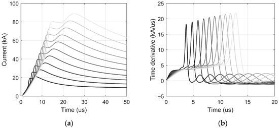
Figure 1.
Double-peaked return-stroke currents synthesized via a multi-component Heidler function method parameterized from Morro do Cachimbo measurements. (a) Simulated waveforms for varying first peak amplitudes; (b) Associated time derivatives illustrating steepness and waveform structure variability relevant to insulation stress.
These relationships, obtained via least squares fitting over a broad range of waveform scenarios, are given by:
2.3.2. Transmission System Modeling
The full transmission system—including phase conductors, shield wires, towers, insulation, and grounding—was modeled in ATP-EMTP. Electromagnetic coupling between conductors was incorporated using the J. Martí line model [5], which captures frequency-dependent behavior through convolution-based line equations.
To ensure accurate propagation of traveling surges and reduce boundary reflections and ensure accurate propagation of traveling surges, the simulation domain was extended beyond the region of interest. Specifically, three additional spans were inserted on either side of the tower subjected to the lightning stroke, and a 5 km line extension was appended to the end of the system. This configuration helps absorb incoming and reflected waves without artificially altering their amplitude or timing.
The transmission towers were modeled as lossless vertical multiconductor structures, segmented into four vertical sections associated with the shield wire and each of the three phase conductors. Each segment was characterized by its vertical length and an equivalent surge impedance calculated using the revised Jordan method proposed by De Conti et al. [36], a formulation widely accepted for lattice towers up to 60 m in height.
For each segment, the effective surge impedance was computed by considering a reference conductor surrounded by three adjacent vertical conductors placed symmetrically in a square configuration. The mutual distances between conductors were set according to the geometry at each tower level, with horizontal spacings derived from the lattice widths and diagonal distances given by the Euclidean norm. The self-impedance of the reference conductor (denoted Z11) is given by:
The mutual impedance between conductor 1 and any adjacent conductor j is expressed as:
The equivalent surge impedance of the segment is then given by the average:
where
- h: height of the segment under consideration,
- r: equivalent radius of the tower leg (vertical conductor),
- d1j: horizontal or diagonal spacing between conductor 1 and conductor j,
- n = 4: number of vertical conductors used in the model.
Diagonal members and crossarms were not explicitly modeled, in accordance with the simplifications proposed in [36]. The wave propagation speed along the tower was set to 0.8c, consistent with measured values for steel lattice towers with bracing and structural complexity [37,38].
2.3.3. Insulation Modeling
The breakdown of insulator strings under lightning-induced transients is governed by both the magnitude of voltage stress and the duration of exposure [8]. Several modeling approaches have been proposed to describe this time-dependent dielectric behavior:
- Volt-time curves (VTCs) [24]
- Disruptive Effect (DE) method (also known as the integration method) [7,39]
- Leader progression models [40,41].
Volt-time curves provide an empirical relationship between the withstand voltage of the insulator and the time to breakdown. These are widely used in engineering practice due to their simplicity and established parameter sets. In contrast, the DE method integrates the effect of the applied voltage over time, and leader progression models seek to explicitly simulate the physical development of streamers and leaders along the insulator surface. While the latter offer higher fidelity, they are data-intensive and require parameters that are not always readily available.
Sarajcev [9] compared these methods and observed that volt-time characteristics—particularly those defined in [24]—may overestimate BFRs in some scenarios. The DE method, in contrast, was found to agree more closely with leader progression models. Nevertheless, due to its practicality and historical usage in insulation coordination studies, the volt-time curve approach was adopted in this work.
The flashover strength Vf as a function of time to breakdown t is described by:
where
- Vf is the critical withstand voltage at time t (in kV),
- k and n are empirical constants derived from laboratory testing.
In this study, a specific withstand function recommended by IEEE Std 1243 [2] was used:
where t is the time to flashover in microseconds and W is the gap or insulator length in meters. This expression follows the general form in Equation (36) but provides parameter values validated for high-voltage systems. It has been widely adopted in transmission line insulation coordination studies due to its practical accuracy and standardization.
2.3.4. Grounding System Representation
The grounding system plays a central role in determining the severity of lightning-induced overvoltages, particularly during backflashover events. Various modeling techniques have been proposed to describe their transient behavior, ranging from lumped-resistance circuit models [42] to full-wave electromagnetic solvers [43].
Each class of models involves a balance between accuracy and computational requirements. Full-wave formulations directly solve Maxwell’s equations, necessitating detailed information about soil geometry and material properties, but they often demand significant computational resources. Simplified circuit-theory models, on the other hand, represent the grounding system as a fixed resistance and do not account for frequency-dependent impedance behavior, allowing for parametric studies with lower complexity.
A central aspect in the accurate modeling of grounding systems is the frequency dependence of soil electrical properties, particularly conductivity and permittivity. These parameters vary significantly across the lightning frequency spectrum and influence how transient currents dissipate into the soil [44]. Among the available models, the Alipio–Visacro Model (AVM) [45] has been extensively validated and provides a robust characterization of soil impedance as a function of frequency.
Despite the accuracy of such models, this study adopts a parametric approach in which the tower-footing impedance Zp is treated as a fixed input rather than derived from first principles. This method, following the precedent established by Silveira and Visacro [46], allows the analysis to remain general and broadly applicable across varying site conditions.
Specifically, simulations were performed for discrete values of Zp ranging from 10 Ω to 40 Ω, covering typical values encountered in field measurements. This approach offers several advantages:
- It eliminates dependence on site-specific soil characterization, which may be unavailable or highly uncertain.
- It allows a direct sensitivity analysis of grounding conditions on backflashover performance.
- It supports generalizability, making the results relevant across a broad range of installations.
In each simulation case, Zp was treated as a constant boundary parameter in the ATP-EMTP model, enabling systematic assessment of its impact on flashover probability without requiring detailed grounding grid modeling.
2.4. Monte Carlo Simulation for Backflashover Probability
The BFR is numerically estimated using a Monte Carlo simulation that operationalizes the probabilistic framework introduced in Section 2.1. Each simulation trial represents a unique lightning event characterized by randomly sampled stroke parameters, enabling stochastic assessment of interception and subsequent flashover on the transmission line. Each iteration involves two primary steps: (i) determination of stroke interception based on the selected attachment model and (ii) flashover evaluation based on the induced transient overvoltage.
2.4.1. Random Sampling of Parameters
Each Monte Carlo iteration independently samples the following parameters:
- Return-stroke peak current (I): Sampled from a log-normal distribution calibrated using measurements from the Morro do Cachimbo lightning station in Brazil [33,34]. This parameter influences both the lateral interception distance and, together with the correlated rise time, the surge magnitude.
- Lateral stroke position (x): Uniformly distributed within a ±500 m corridor centered on the transmission line, representing the horizontal displacement of the downward leader channel relative to the tower.
- System voltage phase angle (φ): Uniformly sampled within [0, 2π], representing the instantaneous phase of the power-frequency voltage at the moment of the stroke. It impacts the superposition of steady-state and surge voltages and hence the likelihood of flashover.
These parameters define the stochastic realization (I(i), x(i), φ (i)) for the i-th trial.
2.4.2. Stroke Attachment Evaluation
Stroke interception depends on the adopted attachment model:
- Eriksson Empirical Model [3]: Interception is assumed for all strokes within the deterministic average attractive radius calculated from Equation (6).
- Electrogeometric Models [2,20,21,22,23,24,25]: Striking distances to ground, shield wire, and phase conductors are computed based on current I. A stroke is intercepted if its lateral stroke position falls within the shield wire exposure distance as calculated with Equations (A5) and (A6).
- Simulation-Based Leader Progression Model (SB-LPM): A stroke is intercepted if ⏐x⏐ ≤ R(I), with R(I) being the attractive radius in Equation (21), derived from detailed attachment simulations as described in Section 2.2.3 and presented in Section 3.2.
An indicator function δ(i)attach∈{0,1} identifies successful interception for each stroke.
2.4.3. Flashover Evaluation and BFR Estimation α
For each intercepted stroke, an ATP-EMTP simulation is executed following the modeling approach detailed in Section 2.3. The sampled return-stroke waveform is injected at the shield wire at the tower top, and the resulting overvoltage across the insulator is computed. Flashover is recorded if this overvoltage exceeds the insulation withstand level, producing a second indicator function δ(i)flashover∈{0,1}.
The Monte Carlo-derived numerical approximation of the BFR, consistent with the probabilistic framework introduced in Section 2.1, is:
Here:
- N is number of iterations;
- δ(i)attach: indicates whether stroke i was intercepted by the shield wire;
- δ(i)flashover indicates whether flashover occurred, given interception;
- Ksf is the span factor (assumed equal to 0.6);
- Ng is the GFD (normalized to 1 flash/km2/year);
- w is the width of the evaluated strike zone (1 km)
- L is the transmission line length, chosen as 100 km.
As N → ∞, this estimate converges to the analytical integral defined in Equation (1).
- Statistical Convergence Criterion
Convergence of the BFR estimate is monitored through the coefficient of variation (βBFR):
where E[BFR] and V[BFR] are the sample mean and variance, respectively. Simulation terminates once:
This criterion ensures a maximum relative uncertainty of 5%. Convergence behavior depends on model characteristics, particularly the presence of stochastic leader attachment and is further discussed in Section 3.5.
3. Results
3.1. Case Study: Backflashover Performance of the 138 kV MC-VP Transmission Line
The methodology described in Section 2 was applied to evaluate the BFR for the Montes Claros–Várzea da Palma (MC-VP) 138 kV transmission line, located in Minas Gerais, Brazil. The MC-VP system is a single-circuit line supported by steel lattice towers, featuring a single overhead shield wire. The transmission line geometry used for simulations is depicted in Figure 2, and conductor characteristics are provided in Table 1.
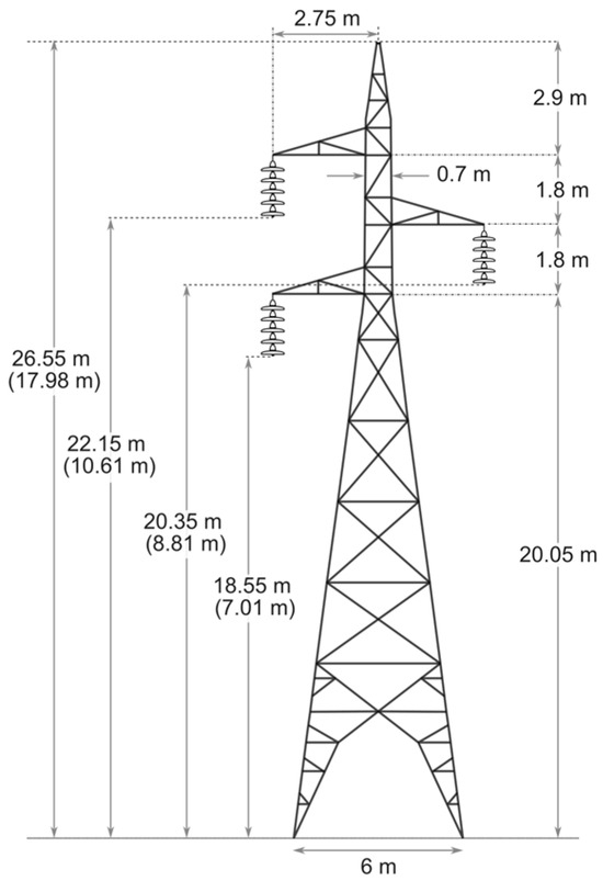
Figure 2.
Transmission line configuration for the 138 kV case study, showing the tower layout and conductor geometry. Values in parentheses indicate midspan heights, which influence lightning exposure and surge propagation.

Table 1.
Electrical and physical properties of the phase conductor and shield wire used in the 138 kV transmission line model.
Key transmission line characteristics include:
- Average span length: 333 m
- Insulator string length: 1.504 m (utility data)
- Lightning impulse withstand voltage: 650 kV (IEC/EN standardized value for 138 kV-class lines; also reported in the literature for similar test lines as critical flashover voltage (CFO), e.g., [46]).
- Phase conductor sag: 11.54 m
- Shield wire sag: 8.57 m
All BFR and flash collection rate (FCR) results presented are normalized to a standard ground flash density of Ng = 1 flash/km2·year, facilitating comparison across diverse transmission line configurations and modeling scenarios.
3.2. Simulation-Derived Attractive Radius
Figure 3 illustrates the COMSOL Multiphysics environment employed to estimate the attractive radius of the 138 kV transmission line tower using the Simulation-Based Leader Progression Model (SB-LPM) developed in this work. The simulation domain includes a detailed 3D representation of the tower and shield wire arrangement, embedded within an ambient volume where the electric field intensification is computed under varying stepped leader conditions.
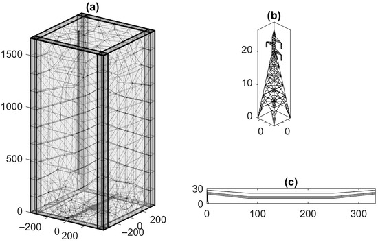
Figure 3.
COMSOL–MATLAB simulation setup for attractive radius estimation using the Simulation-Based Leader Progression Model (SB-LPM): (a) Meshed simulation domain including the stepped leader, transmission line structure, and ambient volume; (b) Transmission tower geometry (conductors omitted for clarity); (c) Full-span configuration displaying conductor sag and shield wire layout.
The attractive radius R(I) for each return-stroke current was determined following Section 2.2.3 by identifying the maximum lateral leader offset allowing successful leader interception. The resulting dataset was fitted to a power-law:
where R(I) is in meters and I in kiloamperes. The data points and fitted curve are shown in Figure 4.
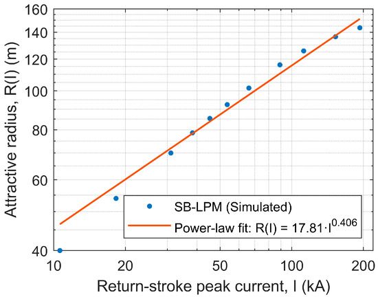
Figure 4.
Attractive radius R(I) versus return-stroke peak current I for the test 138 kV transmission line using the Simulation-Based Leader Progression Model (SB-LPM). Blue circles indicate simulated data points; the red curve shows the fitted power-law expression R(I) = 17.81·I0.406, used in the Monte Carlo simulations.
3.3. Lightning Exposure Estimation
Figure 5 compares attractive radii predicted by the SB-LPM with striking distance-based exposure distances derived from various Electrogeometric Models (EGMs) [2,20,21,22,23,24,25], covering return stroke currents from 2 to 300 kA. Eriksson’s empirical formulation yields a fixed effective radius of approximately 111.6 m (at the nominal median return-stroke current of 30 kA) for the 26.55 m test tower.
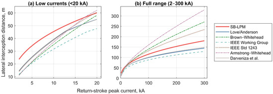
Figure 5.
Comparison of lightning exposure estimates from the Simulation-Based Leader Progression Model (SB-LPM, this work) and six Electrogeometric Models (EGMs) [2,20,21,22,23,24,25], for the test tower geometry. (a): Low-current regime (<20 kA); (b) Full return-stroke current range (2–300 kA); The SB-LPM curve corresponds to a power-law fit of attractive radius values derived from electrostatic simulation and leader inception and propagation modeling. In contrast, EGMs compute exposure distances by applying geometry-based interception logic based on empirically defined striking distances.
3.4. Backflashover Analysis
Tower grounding performance critically influences backflashover probability. Prior studies estimated an impulse grounding impedance of approximately 20.12 Ω for the 138 kV line [47] using frequency-dependent soil parameters derived via the Alípio–Visacro method [45]. This value serves as a representative benchmark; however, to account for the variability of grounding conditions observed in the field, a parametric sweep was performed over impedance values from 10 Ω to 40 Ω. This range is consistent with values observed in field studies and with the approach adopted by Silveira and Visacro [46], who showed that impulse impedances between 10 and 40 Ω yield backflashover estimates comparable with those obtained using more detailed physical models of grounding electrodes. This supports the practical validity of the simplification of using impedance values in lightning performance simulations.
ATP-EMTP Monte Carlo simulations incorporating regionally representative lightning waveforms and the full transient response of the transmission line estimated a BFR of ~6.982 backflashovers/100 km-year at 20 Ω impedance using the SB-LPM.
Figure 6 summarizes BFR, FCR, and critical flashover current (CFC) across tower-footing impedance values for all eight attachment models, including the proposed SB-LPM. In this analysis, the CFC for each impedance value is defined as the lowest lightning return-stroke current in the set of Monte Carlo trials that results in a simulated backflashover event. Throughout the simulation, this value is continuously updated by recording the minimum current associated with a flashover occurrence. This approach ensures that the CFC reflects the most sensitive (i.e., lowest-current) flashover observed for each model under the sampling conditions of the Monte Carlo analysis.
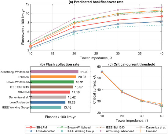
Figure 6.
Backflashover performance metrics for different attachment models across varying tower-footing impedances: (a) Flash Collection Rate (FCR); (b) Backflashover Rate (BFR), and (c) Critical Flashover Current (CFC). The results underscore the influence of attachment model choice and grounding impedance on predicted backflashover risk.
Table 2 summarizes the percentage change in FCR and BFR at 20 Ω for each attachment model relative to the Eriksson formulation. The SB-LPM predicts a 14.2% reduction in flash collection and a 9.9% reduction in BFR, reflecting the influence of its physics-based leader modeling. While some models (e.g., Armstrong–Whitehead) show higher collection and flashover rates, others—including the IEEE Working Group and Love/Anderson formulations—predict significantly lower exposure and flashover estimates. These variations underscore the impact of attachment model choice on the estimated lightning performance of transmission lines.
Table 2.
Percentage change in flash collection rate (FCR) and backflashover rate (BFR) relative to Eriksson’s model.
3.5. Monte Carlo Convergence Analysis
Statistical convergence for BFR estimates was assessed using the coefficient of variation (βBFR), with a threshold of 0.05 for termination (corresponding to a maximum relative uncertainty of 5%).
Figure 7 shows convergence behaviors:
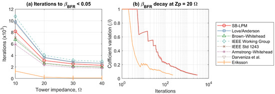
Figure 7.
(a) Number of Monte Carlo iterations required to reach convergence (βBFR < 0.05), versus tower-footing impedance for all considered attachment models: Simulation-Based Leader Progression Model (SB-LPM), six electrogeometric models (EGMs) [2,20,21,22,23,24,25] and Eriksson [3]; (b) Decay of the convergence metric βBFR versus iteration count at 20 Ω, shown for the SB-LPM and Eriksson. The Eriksson model converges rapidly due to deterministic interception, while the LPM requires substantially more iterations due to stochastic rejection of non-intercepting strokes.
- Panel (a): iterations required to reach convergence across tower-footing impedance for all attachment models. This comprehensive comparison highlights the considerable variability in convergence effort associated with different stroke incidence formulations.
- Panel (b): evolution of the convergence metric βBFR at 20 Ω for two representative models: SB-LPM and Eriksson’s empirical model [3].
3.6. Computational Cost
To illustrate the computational requirements of the proposed framework, the main processing steps and their typical execution times are summarized below:
- Hardware: Intel® Core™ i7-4600U, 2.7 GHz, 8 GB RAM
- Attachment simulations (COMSOL): Each current offset case required ~7–8 min of processing. In total, ~100 cases were run across 11 current levels (Figure 4), corresponding to a processing effort of ~20 h.
- ATP-EMTP transient runs: ~2.1–2.5 s each, managed via MATLAB including I/O.
- Monte Carlo BFR estimation (20 Ω footing impedance): ~1149–1288 s for EGMs, ~1090 s for SB-LPM, and ~480 s for Eriksson.
The FEM campaign is performed once to obtain the fitted R(I); the Monte Carlo BFR estimation then employs this function similarly to conventional EGM/Eriksson methods, without additional FEM overhead.
4. Discussion
This section interprets the numerical results presented in Section 3.2, Section 3.3, Section 3.4 and Section 3.5 in the context of lightning attachment theory and backflashover performance of high-voltage transmission lines.
4.1. Exposure Predictions of the Simulation-Based Leader Progression Model
At low return-stroke currents (<20 kA), the SB-LPM predicts attractive radii up to approximately 25% larger than those estimated by most EGMs, highlighting an increased impact of tower-geometry-induced field intensification and leader inception thresholds under lower field conditions. Between 20 and 100 kA, SB-LPM results align closely with IEEE Std 1243 [2] but show higher values compared to IEEE Working Group [24], Love/Anderson [22,23], and Darveniza et al. [25], while deviating below the predictions of Brown–Whitehead [21] and Armstrong–Whitehead [20]. For currents above 100 kA, SB-LPM diverges from IEEE Std 1243 and predicts progressively smaller lateral interception than the Whitehead models, indicating a saturation effect in upward leader development not accounted for by empirical EGMs.
The SB-LPM modeling approach, which relies on electrostatic solutions and inception criteria instead of an assumed power law, remains sensitive to transmission line configuration—indicating it can be especially well-suited for lines with unconventional designs.
4.2. Influence of Tower-Footing Impedance and Attachment Model on Backflashover Risk
The backflashover rate (BFR) increases monotonically with tower-footing impedance for every attachment model. This trend reflects the reduced capacity of higher-impedance footings to dissipate surge currents into the soil, increasing the overvoltage stress on the insulation.
Significant variation in BFR is observed between models across the impedance sweep. At lower impedances (10–20 Ω), BFR estimates range from approximately 2.254 to 9.239 backflashovers/100 km-year, revealing strong model dependence even under favorable grounding conditions; beyond 30 Ω, divergence between models becomes more pronounced, with the spread exceeding 4.06 events at 40 Ω. The Simulation-Based LPM predicts consistently lower BFRs than the Eriksson reference [3], with the relative difference becoming more pronounced above 30 Ω and peaking at 40 Ω, where the SB-LPM yields a BFR relative reduction of approximately 12.8%. This difference stems from two compounding effects: (i) a lower flash collection rate (FCR) (17.18 vs. 20.03 flashes/100 km-year) and (ii) marginally higher critical flashover currents (CFCs) in the 20–40 Ω range. These factors jointly reduce the predicted frequency and severity of potentially disruptive surges imposed on the insulation.
The CFC decreases with increasing impedance for all models, as expected from surge reflection behavior and insulation response. In the 20–40 Ω range, the Eriksson model yields slightly higher values than the other models, including the SB-LPM. This behavior likely results from its faster statistical convergence, which reduces the number of trials sampling high-current strokes near the flashover threshold. As a result, the estimated CFC is based on fewer marginal events and may be slightly biased upward. More generally, variations in CFC across attachment models are influenced both by the physical and geometric principles embodied in each model, which determine the population of intercepted lightning strokes, and by the statistical characteristics of the Monte Carlo sampling. The faster convergence behavior of the Eriksson model is further discussed in Section 4.3.
The SB-LPM occupies a central position in terms of the conservatism of the predicted BFR. Among the models evaluated, the Armstrong–Whitehead and IEEE Working Group formulations define the upper and lower bounds, respectively, predicting the highest and lowest BFRs. The remaining models—Eriksson, IEEE Std 1243, Brown–Whitehead, Darveniza et al., and Love/Anderson—cluster around the SB-LPM with varying biases. Eriksson, IEEE 1243, and Brown–Whitehead generally yield moderately higher BFRs than the SB-LPM, with Eriksson slightly lower at low impedances but crossing above near 25–30 Ω. In contrast, Darveniza et al. and Love/Anderson consistently produce slightly lower BFRs than the SB-LPM across the evaluated impedance range.
These findings underscore the SB-LPM’s value as a balanced benchmark for assessing the relative conservatism of lightning attachment models. They also demonstrate that incorporating physics-based leader modeling can moderate overly conservative predictions while maintaining appropriate safety margins.
Recent developments have introduced simplified procedures based, e.g., on the Rizk attachment model, such as the approach presented in CIGRE TB 839 [1]. These procedures are primarily intended for extra-high voltage (EHV) and ultra-high voltage (UHV) systems, and their validation has focused on shielding failure rate rather than backflashover rate. As such, their direct applicability to the 138 kV case examined here is limited.
4.3. Monte-Carlo Convergence and Computational Cost
Eriksson’s model achieves rapid convergence due to a deterministic interception criterion, considering all strokes within a defined fixed attractive radius as successful attachments (βBFR values typically falling below 0.05 within several hundred trials). In contrast, the SB-LPM and the six evaluated EGMs introduce stochastic rejection mechanisms, with attachment outcomes depending on random sampling of leader position and probabilistic criteria. This inherently increases estimator variance, especially at lower tower impedances where backflashover events are infrequent.
For instance, SB-LPM requires approximately 7800 iterations at 10 Ω and 3800 at 20 Ω to meet the same statistical confidence level. While this represents an order-of-magnitude increase in computational effort relative to the Eriksson model, the overhead remains manageable. More importantly, it is justified by the improved physical realism introduced by the SB-LPM framework.
4.4. Practical Implications and Outlook
The SB-LPM framework offers balanced and geometry-sensitive predictions, establishing it as a promising approach for backflashover rate estimation—particularly when tower designs or grounding conditions exceed the empirical bounds of classical EGMs.
Looking ahead, several avenues will further enhance the methodology’s scope and impact:
- Initial application at 138 kV: this study demonstrates the SB-LPM framework at the 138 kV level, providing insight into its distinct predictive behavior compared to electrogeometric models, even at a “standard” transmission voltage. However, results at this level do not capture all complexities of higher-voltage systems and should not be viewed as fully generalizable.
- Broader system coverage: Future work will extend SB-LPM to a wider range of tower heights, conductor configurations, and terrain profiles through expanded simulation campaigns and benchmarking.
- Span-level attachment modeling: While the present study focused on the attractive radius concept and lateral attachment domain for comparison with EGMs, the explicit representation of the span in both COMSOL and ATP provides a strong foundation for distinguishing longitudinal (span versus tower) interception events in future research. Incorporating this additional dimension represents a promising direction for extending the SB-LPM framework.
- Higher-voltage and HVDC applications: EHV and HVDC systems present additional complexities—including longer insulation strings, advanced shielding practices, and distinct transient phenomena—that merit targeted investigation. Extending SB-LPM to these voltage classes, especially as HDVC grows in importance for renewable energy integration and large-grid interconnection, is a principal ongoing research direction.
- Comparisons with additional attachment models: Future extensions may also be considered in future extensions of the framework, such as the Rizk-based simplified procedure in CIGRE TB 839, which is particularly suited for EHV and UHV lines. Including such methods in comparative studies at higher voltages would further broaden the benchmarking of attachment models within the SB-LPM framework.
- Lightning current statistics: The recent modeling-based correction of the Morro do Cachimbo measurements [35] illustrates how tower and terrain attractivity can bias measured distributions, yielding decontaminated current statistics (frequency and cumulative) with a lower median (~33 kA compared to ~43 kA in the original dataset) and a reduced frequency of extreme values. Once consolidated and accompanied by the parameter correlations required for waveform synthesis, such distributions could be incorporated into the framework to further refine BFR estimates.
- Computational efficiency: Adoption of surrogate modeling, parametrized meshing, and automated geometry generation will support broader applicability and lower the computational burden of flash incidence simulations.
- Advanced probabilistic methods: Integrating adaptive sampling and variance-reduction techniques will further enhance Monte Carlo simulation efficiency for backflashover risk quantification.
Collectively, these efforts will enable SB-LPM to provide robust, routine lightning performance assessments and inform design optimization for a broad array of existing and emerging transmission technologies, including EHV and HVDC lines.
5. Conclusions
This paper introduced a probabilistic framework for estimating backflashover rates (BFRs) in high-voltage transmission lines subjected to lightning strikes. The approach integrates physics-based stroke incidence modeling, lightning-induced transient simulations, and stochastic assessment of flashover risk. Central to this framework is the Simulation-Based Leader Progression Model (SB-LPM), which leverages electrostatic simulations to model streamer inception, upward leader propagation, and lightning attachment dynamics, providing an alternative to traditional empirical models with enhanced predictive accuracy.
- Key Findings
Application of this framework to a representative 138 kV transmission line revealed critical insights into lightning performance modeling:
- The choice of lightning attachment model—particularly whether interception is modeled deterministically or probabilistically—significantly influences both the predicted BFR and the computational resources required for statistically reliable estimates;
- Monte Carlo convergence analysis demonstrated that deterministic attachment models, such as Eriksson’s formulation, achieve faster statistical convergence due to simplified interception criteria. Conversely, the SB-LPM requires increased computational effort to accurately resolve the stochastic nature of leader interception and flashover processes. This highlights an inherent trade-off between model accuracy and computational efficiency;
- SB-LPM consistently predicted lower BFR estimates compared to the Eriksson model, especially at higher tower-footing impedances. This difference arises because SB-LPM’s detailed stochastic representation of leader attachment leads to variability in the lightning current waveform and precise attachment positions. Consequently, this variability influences the resulting transient overvoltages more substantially at higher impedances, affecting flashover probability;
- Accurate representation of lightning waveform characteristics, detailed modeling of transmission system elements, and integration of realistic lightning statistics emerged as critical components for reliable lightning performance assessment;
- Finite element electrostatics-derived attractive radii offer physically consistent modeling of lightning attachment, capturing geometry-specific exposure dynamics effectively;
- Among evaluated attachment models, SB-LPM offers a balanced benchmark in terms of BFR conservatism—positioned between the upper bound defined by Armstrong–Whitehead and the lower bound set by the IEEE Working Group model. This underscores its value in moderating overly conservative predictions through physics-based leader modeling.
The conclusions drawn here apply to high-voltage transmission systems in the 69–230 kV range. While the present study was demonstrated on a single 138 kV configuration, the framework can be expanded to other line geometries and, in future work, to extra-high-voltage (EHV) and HVDC systems. Its application may also be broadened to encompass different grounding conditions and lightning current datasets. Overall, the proposed integrated, physics-based approach provides a solid foundation for advancing lightning performance assessment, offering a flexible and practical toolset for reliability studies in transmission system design.
Author Contributions
Conceptualization, A.T.L., R.A.R.M., L.A., M.A.O.S. and V.C.; methodology, A.T.L. and R.A.R.M.; software, A.T.L. and R.A.R.M.; validation, R.A.R.M., L.A., M.A.O.S. and V.C.; formal analysis, A.T.L.; investigation, A.T.L.; resources, R.A.R.M., M.A.O.S. and V.C.; data curation, A.T.L.; writing—original draft preparation, A.T.L.; writing—review and editing, R.A.R.M., L.A., M.A.O.S. and V.C.; visualization, A.T.L.; supervision, L.A., M.A.O.S. and V.C.; project administration, A.T.L., L.A. and M.A.O.S.; funding acquisition, A.T.L. and V.C. All authors have read and agreed to the published version of the manuscript.
Funding
A.L. was supported by the National Council for Scientific and Technological Development, CNPq—Brazil, grant number 201375/2014-1.
Data Availability Statement
The key data supporting the findings are included within the article. Further inquiries can be directed to the corresponding author.
Acknowledgments
The authors acknowledge the institutional support of Uppsala University and the Federal University of São João del-Rei (UFSJ).
Conflicts of Interest
Author Liliana Arevalo was employed by the Hitachi Energy Sweden AB. The remaining authors declare that the research was conducted in the absence of any commercial or financial relationships that could be construed as a potential conflict of interest. The funders had no role in the design of the study; in the collection, analyses, or interpretation of data; in the writing of the manuscript; or in the decision to publish the results.
Abbreviations
The following abbreviations are used in this manuscript:
| BFR | Backflashover Rate |
| CFC | Critical Flashover Current |
| EGM | Electrogeometric Model |
| EHV | Extra-High Voltage |
| FCR | Flash Collection Rate |
| GFD | Ground Flash Density |
| LPM | Leader Progression Model |
| SB-LPM | Simulation-Based Leader Progression Model |
| UHV | Ultra-High Voltage |
Appendix A. Electrogeometric Models (EGMs)
Electrogeometric models (EGMs) describe the lightning attachment process in terms of the striking distance, defined as the final gap between a descending stepped leader and a structure at the moment of attachment. Attachment occurs when the electric field across this gap exceeds the breakdown threshold of air [4].
The striking distance to an elevated conductor (e.g., shield wires, phase conductors), denoted rc is generally expressed as a power-law function of the return-stroke peak current (I) [1,2]:
To account for reduced field enhancement at ground level, the striking distance to the ground surface, rg, is scaled by a factor β ≤ 1:
Parameters A, b and β are empirically derived from laboratory and field measurements. They vary among different EGM formulations depending on factors such as voltage level, tower configuration, and terrain. Representative values from widely used and well-known EGMs are summarized in Table A1.
Table A1.
Empirically derived parameters A, b, and β for selected electrogeometric models.
Table A1.
Empirically derived parameters A, b, and β for selected electrogeometric models.
| Source | Striking Distance Parameters | ||||
|---|---|---|---|---|---|
| A | b | β | β (230–765 kV) | β (>765 kV) | |
| Armstrong–Whitehead [20] | 6.7 | 0.8 | 0.9 | — | — |
| Brown–Whitehead [21] | 7.1 | 0.75 | 0.9 | — | — |
| Love [22] | 10 | 0.65 | 1 | — | — |
| Darveniza at al [25] | 9.4 | 0.67 | 1 | — | — |
| Anderson [23] | 10 | 0.65 | 1 | 0.8 | 0.67 |
| IEEE Working Group [24] | 8 | 0.65 | 1 | 0.8 | 0.64 |
| IEEE Std 1243 [2] | 10 | 0.65 | f(y) 1 | — | — |
1 IEEE Std 1243 defines the height-dependent function β = 0.36 + 0.17 ln(43 − y) for y < 40 m and β = 0.55 for y ≥ 40 m, where y is the average conductor height (tower height minus two-thirds of the mid-span sag).
Appendix A.1. EGM Application in Shielding and Backflashover Analyses
Love’s striking distance equation [22] is widely considered a fundamental EGM and serves as the basis for several derivative formulations, such as those by Anderson [23] and IEEE Std 1243 [2]. These later adaptions introduce voltage-dependent and height-dependent corrections to the ground scaling factor β.
The CIGRE Working Groups 33.01 [1] and C4.23 [11] recommends the Brown-Whitehead formulation [21] due to its ability to the represent a reasonably severe attachment condition.
The IEEE Working Group [24] introduced a striking distance equation representing a 20% reduction compared to Love’s original formulation. This equation was intended to reflect the minimum rather than average striking distance for a given peak current [48]. However, inconsistences between this formulation and observed stroke incidence led to the return to Love’s original equation and the adoption of a height-dependent β [48] to reconcile EGM striking distances with those predicted by stroke incidence models such as Eriksson’s [3] and Rizk’s [13]. This height-dependent correction was later incorporated into IEEE Std 1243 and has been extensively adopted.
Notably, IEEE Std 998, used for substation shielding assessments [49], employs the shorter striking distance equation from the IEEE Working Group.
EGMs are primarily applied in transmission line shielding analysis. Conversely, Eriksson’s empirical model, employing an average attractive radius (Equation (6)), is typically utilized to estimate the total number of lightning strikes to shield wires, forming the basis of subsequent backflashover analysis [1,2].
Nevertheless, EGMs have also been effectively utilized in Monte Carlo or EMTP-ATP-based backflashover studies [9,10,50]. In such analyses, IEEE Std 1243’s striking distance and height-dependent β are most commonly adopted.
Appendix A.2. Exposure Distances and Flash Collection Rate
The striking distance equations enable the calculation of lateral the exposure distances Dg and Dg′, defining the interception ranges for strokes intercepted by shield wires based on peak current and tower geometry. The maximum shielding failure current, Im, represents the minimum current required for effective shielding by the shield wire, calculated from the corresponding striking distance to ground, rgm, using [51]:
from which:
For currents I ≤ Im, exposure distance Dg(I) is [51]:
For currents above Im, exposure distance Dg′(I) is [52]:
In Equations (A3)–(A6), h is the shield wire height above ground, y the phase conductor height, and a the horizontal spacing between shield wire and phase conductor.
Finally, the FCR is determined by integrating the exposure distances over the return-stroke current distribution:
References
- CIGRE Working Group 33.01. Guide to Procedures for Estimating the Lightning Performance of Transmission Lines; Technical Brochure 63, Reissued 2021; CIGRE: Paris, France, 2021; pp. 1–92. [Google Scholar]
- IEEE Std 1243-1997; IEEE Guide for Improving the Lightning Performance of Transmission Lines. Transmission and Distribution Committee of the IEEE Power Engineering Society: Piscataway, NJ, USA, 1997; pp. 1–44.
- Eriksson, A.J. The Incidence of Lightning Strikes to Power Lines. IEEE Trans. Power Deliv. 1987, 2, 859–870. [Google Scholar] [CrossRef]
- Cooray, V.; Rakov, V.; Theethayi, N. The Lightning Striking Distance—Revisited. J. Electrost. 2007, 65, 296–306. [Google Scholar] [CrossRef]
- Marti, J.R. Accurate Modelling of Frequency-Dependent Transmission Lines in Electromagnetic Transient Simulations. IEEE Trans. Power Appar. Syst. 1982, PAS-101, 147–157. [Google Scholar] [CrossRef]
- De Conti, A.; Visacro, S. Analytical Representation of Single- and Double-Peaked Lightning Current Waveforms. IEEE Trans. Electromagn. Compat. 2007, 49, 448–451. [Google Scholar] [CrossRef]
- Darveniza, M.; Vlastos, A.E. The Generalized Integration Method for Predicting Impulse Volt-Time Characteristics for Non-Standard Wave Shapes—A Theoretical Basis. IEEE Trans. Electr. Insul. 1988, 23, 373–381. [Google Scholar] [CrossRef]
- IEEE Std 1410-2010; IEEE Guide for Improving the Lightning Performance of Electric Power Overhead Distribution Lines. Transmission and Distribution Committee of the IEEE Power Engineering Society: Piscataway, NJ, USA, 2010.
- Sarajcev, P. Monte Carlo Method for Estimating Backflashover Rates on High Voltage Transmission Lines. Electr. Power Syst. Res. 2015, 119, 247–257. [Google Scholar] [CrossRef]
- Datsios, Z.G.; Mikropoulos, P.N.; Tsovilis, T.E.; Angelakidou, S.I. Estimation of the Minimum Backflashover Current of Overhead Lines of the Hellenic Transmission System through ATP-EMTP Simulations Lightning and Power Systems. In Proceedings of the International Colloquium on Lightning and Power Systems (ICLPS), Bologna, Italy, 27–29 June 2016. [Google Scholar]
- CIGRE Working Group C4.23. Procedures for Estimating the Lightning Performance of Transmission Lines—New Aspects; Technical Brochure 839 2021; CIGRE: Paris, France, 2021; pp. 1–111. [Google Scholar]
- Rizk, F.A.M. A Model for Switching Impulse Leader Inception and Breakdown of Long Air-Gaps. IEEE Trans. Power Deliv. 1989, 4, 596–606. [Google Scholar] [CrossRef]
- Rizk, F.A.M. Modeling of Transmission Line Exposure to Direct Lightning Strokes. IEEE Trans. Power Deliv. 1990, 5, 1983–1997. [Google Scholar] [CrossRef]
- Dellera, L.; Garbagnati, E. Lightning Stroke Simulation by Means of the Leader Progression Model—I: Description of the Model and Evaluation of Exposure of Free-Standing Structures. IEEE Trans. Power Deliv. 1990, 5, 2009–2022. [Google Scholar] [CrossRef]
- Dellera, L.; Garbagnati, E. Lightning Stroke Simulation by Means of the Leader Progression Model—II: Exposure and Shielding Failure Evaluation of Overhead Lines with Assessment of Application Graphs. IEEE Trans. Power Deliv. 1990, 5, 2023–2029. [Google Scholar] [CrossRef]
- Becerra, M. On the Attachment of Lightning Flashes to Grounded Structures. Ph.D. Dissertation, Acta Universitatis Upsaliensis, Uppsala, Sweden, 2008. [Google Scholar]
- Arevalo, L. Numerical Simulations of Long Spark and Lightning Attachment. Ph.D. Dissertation, Acta Universitatis Upsaliensis, Uppsala, Sweden, 2011. [Google Scholar]
- Cooray, V. (Ed.) Lightning Electromagnetics; Institution of Engineering and Technology: London, UK, 2012; ISBN 9781849192156. [Google Scholar]
- Mikropoulos, P.N.; Tsovilis, T.E. Estimation of Lightning Incidence to Overhead Transmission Lines. IEEE Trans. Power Deliv. 2010, 25, 1855–1865. [Google Scholar] [CrossRef]
- Armstrong, H.R.; Whitehead, E.R. Field and Analytical Studies of Transmission Line Shielding. IEEE Trans. Power Appar. Syst. 1968, PAS-87, 270–281. [Google Scholar] [CrossRef]
- Brown, G.W.; Whitehead, E.R. Field and Analytical Studies of Transmission Line Shielding: Part II. IEEE Trans. Power Appar. Syst. 1969, PAS-88, 617–626. [Google Scholar] [CrossRef]
- Love, E.R. Improvements on Lightning Stroke Modeling and Applications to Design of EHV and UHV Transmission Lines. Master’s Thesis, University of Colorado Denver, Denver, CO, USA, 1973. [Google Scholar]
- Anderson, J.G. Lightning Performance of Transmission Lines. In Transmission Line Reference Book, 345 kV and Above; LaForest, J.J., Ed.; Electric Power Research Institute (EPRI): Palo Alto, CA, USA, 1982; pp. 545–598. [Google Scholar]
- Working Group on Lightning Performance of Transmission Lines. A Simplified Method for Estimating Lightning Performance of Transmission Lines. IEEE Trans. Power Appar. Syst. 1985, PAS-104, 918–932. [CrossRef]
- Darveniza, M.; Popolansky, F.; Whitehead, E.R. Lightning Protection of UHV Transmission Lines. Electra 1975, 41, 39–69. [Google Scholar]
- Lobato, A.; Cooray, V.; Arevalo, L. Attractive Zone of Lightning Rods Evaluated with a Leader Progression Model in a Common Building in Brazil. In Proceedings of the 2017 International Symposium on Lightning Protection (XIV SIPDA), Natal, Brazil, 2–6 October 2017; pp. 380–388. [Google Scholar]
- Gallimberti, I. The Mechanism of the Long Spark Formation. J. Phys. Colloq. 1979, 40, C7-193–C7-250. [Google Scholar] [CrossRef]
- Morrow, R.; Lowke, J.J. Streamer Propagation in Air. J. Phys. D Appl. Phys. 1997, 30, 614–627. [Google Scholar] [CrossRef]
- Goelian, N.; Lalande, P.; Bondiou-Clergerie, A.; Bacchiega, G.L.; Gazzani, A.; Gallimberti, I. A Simplified Model for the Simulation of Positive-Spark Development in Long Air Gaps. J. Phys. D Appl. Phys. 1997, 30, 2441–2452. [Google Scholar] [CrossRef]
- Lalande, P.; Bondiou-Clergerie, A.; Bacchiega, G.; Gallimberti, I. Observations and Modeling of Lightning Leaders. Comptes Rendus Phys. 2002, 3, 1375–1392. [Google Scholar] [CrossRef]
- Press, W.H.; Teukolsky, S.A.; Vetterling, W.T.; Flannery, B.P. Root Finding and Nonlinear Sets of Equations. In Numerical Recipes in C: The Art of Scientific Computing; Cambridge University Press: Cambridge, UK, 1992; pp. 347–393. [Google Scholar]
- Oliveira, A.J.; Schroeder, M.A.O.; Moura, R.A.R.; Correia de Barros, M.T.; Lima, A.C.S. Adjustment of Current Waveform Parameters for First Lightning Strokes: Representation by Heidler Functions. In Proceedings of the 2017 International Symposium on Lightning Protection (XIV SIPDA), Natal, Brazil, 2–6 October 2017; pp. 121–126. [Google Scholar]
- Visacro, S.; Soares, A.; Schroeder, M.A.O.; Cherchiglia, L.C.L.; de Sousa, V.J. Statistical Analysis of Lightning Current Parameters: Measurements at Morro Do Cachimbo Station. J. Geophys. Res. Atmos. 2004, 109, 1–11. [Google Scholar] [CrossRef]
- Visacro, S.; Mesquita, C.R.; De Conti, A.; Silveira, F.H. Updated Statistics of Lightning Currents Measured at Morro Do Cachimbo Station. Atmos. Res. 2012, 117, 55–63. [Google Scholar] [CrossRef]
- Visacro, S.; Santos, D.C.S.; Almeida, G.S.; Reis, A.C.A. Decontaminating Peak Current Distributions Using an Electrostatic-by-Step Representation of the Lightning Leaders That Considers the Effect of the Height of the Instrumented Tower and the Ground Relief. In Proceedings of the GROUND’2023 & 10th LPE International Conference on Grounding & Lightning Physics and Effects, Belo Horizonte, Brazil, 9–12 May 2023; Volume 1, pp. 38–42. [Google Scholar]
- De Conti, A.; Visacro, S.; Soares, A.; Schroeder, M.A.O. Revision, Extension, and Validation of Jordan’s Formula to Calculate the Surge Impedance of Vertical Conductors. IEEE Trans. Electromagn. Compat. 2006, 48, 530–536. [Google Scholar] [CrossRef]
- Kawai, M. Studies of the Surge Response on a Transmission Line Tower. IEEE Trans. Power Appar. Syst. 1964, 83, 30–34. [Google Scholar] [CrossRef]
- Motoyama, H.; Matsubara, H. Analytical and Experimental Study on Surge Response of Transmission Tower. In Proceedings of the 2000 Power Engineering Society Summer Meeting (Cat. No.00CH37134), Seattle, WA, USA, 16–20 July 2000; Volume 2, p. 855. [Google Scholar]
- Witzke, R.L.; Bliss, T.J. Surge Protection of Cable-Connected Equipment. Trans. AIEE 1950, 69, 527–542. [Google Scholar] [CrossRef]
- Shindo, T.; Suzuki, T. A New Calculation Method of Breakdown Voltage-Time Characteristics of Long Air Gaps. IEEE Trans. Power Appar. Syst. 1985, PAS-104, 1556–1563. [Google Scholar] [CrossRef]
- Mozumi, T.; Baba, Y.; Ishii, M.; Nagaoka, N.; Ametani, A. Numerical Electromagnetic Field Analysis of Archorn Voltages during a Back-Flashover on a 500-KV Twin-Circuit Line. IEEE Trans. Power Deliv. 2003, 18, 207–213. [Google Scholar] [CrossRef]
- Kherif, O.; Chiheb, S.; Teguar, M.; Mekhaldi, A.; Harid, N. Time-Domain Modeling of Grounding Systems’ Impulse Response Incorporating Nonlinear and Frequency-Dependent Aspects. IEEE Trans. Electromagn. Compat. 2018, 60, 907–916. [Google Scholar] [CrossRef]
- Grcev, L.; Kuhar, A.; Markovski, B.; Arnautovski-Toseva, V. Generalized Network Model for Energization of Grounding Electrodes. IEEE Trans. Electromagn. Compat. 2019, 61, 1082–1090. [Google Scholar] [CrossRef]
- Portela, C. Measurement and Modeling of Soil Electromagnetic Behavior. In Proceedings of the 1999 IEEE International Symposium on Electromagnetic Compatability. Symposium Record (Cat. No.99CH36261), Seattle, WA, USA, 2–6 August 1999; Volume 2, pp. 1004–1009. [Google Scholar]
- Alipio, R.; Visacro, S. Modeling the Frequency Dependence of Electrical Parameters of Soil. IEEE Trans. Electromagn. Compat. 2014, 56, 1163–1171. [Google Scholar] [CrossRef]
- Silveira, F.H.; Visacro, S. Lightning Performance of Transmission Lines: Impact of Current Waveform and Front-Time on Backflashover Occurrence. IEEE Trans. Power Deliv. 2019, 34, 2145–2151. [Google Scholar] [CrossRef]
- de Oliveira, A.J. Transmission Line Performance Under Lightning from a Probabilistic Perspective. Master’s Thesis, Universidade Federal de São João del-Rei, São João del-Rei, Brazil, 2018. (In Portuguese). [Google Scholar]
- Working Group on Estimating the Lightning Performance of Transmission Lines. Estimating Lightning Performance of Transmission Lines. II. Updates to Analytical Models. IEEE Trans. Power Deliv. 1993, 8, 1254–1267. [Google Scholar] [CrossRef]
- IEEE Std 998-2012; IEEE Guide for Direct Lightning Stroke Shielding of Substations. Transmission and Distribution Committee of the IEEE Power Engineering Society: Piscataway, NJ, USA, 2013; pp. 1–227.
- Martínez-Velasco, J.A.; Castrp-Aranda, F. EMTP Implementation of a Monte Carlo Method for Lightning Performance Analysis of Transmission Lines. Ingeniare 2008, 16, 169–180. [Google Scholar] [CrossRef][Green Version]
- Hileman, A.R. Shielding of Transmission Lines. In Insulation Coordination for Power Systems; CRC Press: Boca Raton, FL, USA, 1999; pp. 241–274. ISBN 978-0-8247-9957-1. [Google Scholar][Green Version]
- Hileman, A.R. The Lightning Flash. In Insulation Coordination for Power Systems; CRC Press: Boca Raton, FL, USA, 1999; pp. 195–240. ISBN 978-0-8247-9957-1. [Google Scholar][Green Version]
Disclaimer/Publisher’s Note: The statements, opinions and data contained in all publications are solely those of the individual author(s) and contributor(s) and not of MDPI and/or the editor(s). MDPI and/or the editor(s) disclaim responsibility for any injury to people or property resulting from any ideas, methods, instructions or products referred to in the content. |
© 2025 by the authors. Licensee MDPI, Basel, Switzerland. This article is an open access article distributed under the terms and conditions of the Creative Commons Attribution (CC BY) license (https://creativecommons.org/licenses/by/4.0/).