Rapid Temperature Prediction Model for Large-Scale Seasonal Borehole Thermal Energy Storage Unit

Abstract

The temperature of the thermal energy storage unit is a critical parameter for the stable operation of seasonal borehole thermal energy storage (BTES) systems. However, existing temperature prediction models predominantly focus on estimating single-point temperatures or borehole wall temperatures, while lacking effective methods for calculating the average temperature of the storage unit. This limitation hinders accurate assessment of the thermal charging and discharging states. Furthermore, some models involve complex computations and exhibit low operational efficiency, failing to meet the practical engineering demands for rapid prediction and response. To address these challenges, this study first develops a thermal response model for the average temperature of the storage unit based on the finite line source theory and further proposes a simplified engineering algorithm for predicting the storage unit temperature. Subsequently, two-dimensional discrete convolution and Fast Fourier Transform (FFT) techniques are introduced to accelerate the solution of the storage unit temperature distribution. Finally, the model’s accuracy is validated against practical engineering cases. The results indicate that the single-point temperature engineering algorithm yields a maximum relative error of only 0.3%, while the average temperature exhibits a maximum relative error of 1.2%. After employing FFT, the computation time of both single-point and average temperature engineering algorithms over a 10-year simulation period is reduced by more than 90%. When using two-dimensional discrete convolution to calculate the temperature distribution of the storage unit, expanding the input layer from 200 × 200 to 400 × 400 and the convolution kernel from 25 × 25 to 51 × 51 reduces the time required for temperature superposition calculations to approximately 0.14–0.82% of the original time. This substantial improvement in computational efficiency is achieved without compromising accuracy.

1. Introduction

Building heating systems worldwide have long exhibited a high dependence on fossil fuels, posing significant challenges to both energy security and environmental sustainability. According to the International Energy Agency, space heating in buildings accounts for over 30% of global energy consumption, with approximately 75% of this demand still met by fossil fuel sources [1]. In alignment with the Paris Agreement’s target of limiting global temperature rise to 1.5 °C, many countries are actively accelerating the decarbonization of their heating systems. Electrified heating—particularly technologies based on heat pumps—has emerged as a promising low-carbon solution owing to its high electrothermal conversion efficiency. Nevertheless, during cold seasons, the absence of a stable low-temperature heat source remains a critical bottleneck constraining the large-scale deployment of heat pump systems [2,3,4]. To address the challenge of insufficient heat supply during cold seasons, seasonal thermal energy storage (STES) technologies have gained increasing attention. By integrating multiple heat sources at the regional or urban scale, these systems establish sustainable thermal reserves capable of supplying stable heat during the heating season. STES enables the temporal redistribution of thermal energy across seasons by efficiently storing surplus heat during non-heating periods and releasing it during heating periods. This approach helps balance the thermal energy supply–demand mismatch and mitigate fluctuations in the broader energy system. Among various STES technologies, Borehole Thermal Energy Storage systems (BTES)—which integrate multiple clean heat sources such as solar energy and groundwater to establish a “store in summer, use in winter” recycling model—are increasingly recognized as a promising pathway for achieving clean and sustainable building heating, and have garnered growing attention in recent years [5].

To characterize the heat transfer processes within thermal energy storage units, various modeling approaches have been proposed by researchers. Among numerical models, Carli et al. [6] introduced the Capacity Resistance Model, inspired by electrical resistive network analogies, to predict both the fluid outlet temperature and the temperature of the thermal storage unit. While this model accounts for thermal interference effects between boreholes, it neglects the heat capacity within the boreholes and simplifies the process as steady-state heat conduction. Building upon this work, Bauer et al. [7] introduced the concept of borehole thermal capacity and presented computational results under various operating conditions, including fully transient, borehole transient, and borehole steady-state scenarios, thereby developing the Thermal Resistance and Capacity Model. Although numerical models can accurately predict temperature variations within thermal energy storage units, their computational complexity, slow execution speed, and high demand for computational resources and modeling expertise limit their widespread practical application in engineering contexts.

In contrast, analytical models have garnered increasing attention due to their high computational efficiency [8]. Ingersoll et al. [9] proposed the classical infinite line source model, which assumes a uniform initial ground temperature and treats the borehole as an infinitely long line heat source. Subsequently, Carslaw et al. [10] extended this concept by modeling the borehole as an infinite cylindrical heat source, leading to the development of the infinite cylindrical source model. However, both models neglect the effects of surface boundary conditions, leading to non-convergent temperature fields over extended time scales. As a result, they are unsuitable for long-term thermal performance analysis. To overcome the limitations of previous models, Eskilson [11] developed a finite line source model, while maintaining the assumptions of a uniform initial ground temperature and neglecting the thermal capacity of borehole materials. He further introduced the concept of a dimensionless temperature response factor, known as the g-function. Each g-function corresponds to a specific borehole field configuration, and its thermal response can be precomputed and tabulated for efficient use. These g-function datasets have been widely implemented in geothermal heat pump design tools such as Earth Energy Designer and Ground Loop Heat Exchanger Design Software [12]. However, Eskilson’s g-function is derived through numerical pre-calculation, necessitating the prior generation of a function library tailored to specific geological conditions and borehole configurations. This requirement limits the model’s flexibility and general applicability in diverse engineering scenarios [13].To enhance the practicality of the finite line source models, Zeng [14] employed virtual heat sources and Green’s function methods to derive an analytical solution for finite line heat sources, and proposed a double integral formulation to calculate the average borehole wall temperature. Building on this work, Lamarche [15] improved computational efficiency by reducing the formulation to a single integral through mathematical simplification. Subsequently, Du [16] further optimized the integration sequence and developed a more concise and computationally efficient expression.

In summary, the finite line source model demonstrates clear advantages in computational efficiency over fully three-dimensional numerical models, while adequately accounting for the vertical scale of boreholes and surface boundary effects. Although numerical models yield higher accuracy, their prohibitive computational cost limits their applicability to rapid predictions in large-scale BTES systems. Conversely, the infinite cylindrical source model, despite its concise formulation, neglects surface boundary conditions, resulting in non-convergent temperature fields over extended timescales, which undermines its suitability for seasonal or multi-year storage analysis. By contrast, the finite line source model achieves a rigorous balance between accuracy and efficiency: it incorporates surface effects, retains an analytical solution form, and allows further simplification into engineering-oriented algorithms. Accordingly, this study adopts the finite line source model as the theoretical foundation for establishing a rapid temperature prediction framework.

However, as BTESs evolve toward large-scale, multi-borehole configurations, the volume and complexity of the thermal storage unit increase substantially. Even with simplified analytical formulations, existing models face performance bottlenecks when applied to large-scale scenarios. Furthermore, driven by advancements in clean heating technologies, BTES systems are increasingly being utilized not only for heat extraction but also for thermal energy storage. Under such conditions, relying solely on single-point temperatures or fluid outlet temperatures is no longer sufficient to comprehensively assess the thermal state of the storage unit. This necessitates the development of effective methods for estimating both the average temperature and the spatial temperature field distribution within the thermal storage unit.

To address the aforementioned issues, this study integrates both theoretical modeling and engineering validation. First, a theoretical formulation for calculating the average temperature of the thermal energy storage unit was derived based on the finite line source theory. Second, a simplified engineering algorithm, free from complex functions and integral operations, was developed to enable both single-point temperature calculation and average temperature estimation of the heat storage unit, with the latter derived from an equivalent single-borehole thermal response model. The accuracy of this algorithm was validated through controlled sandbox experiments and real-world engineering data. Finally, a temperature field superposition method based on two-dimensional discrete convolution, enhanced by the fast Fourier transform (FFT), was developed to enable efficient simulation of the temperature distribution in large-scale heat storage bodies.

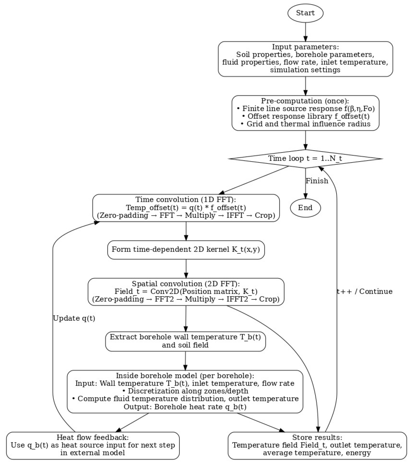
Compared with existing simplified analytical and numerical models such as the g-function approach, TRNSYS, or DST-based tools, the proposed framework offers several novel contributions. First, the model directly integrates the finite line source theory with a two-dimensional convolution formulation, enabling full-field temperature prediction of large-scale BTES units rather than relying solely on point or borehole wall temperatures. Second, by introducing engineering-oriented algorithms, the method eliminates complex integral functions, which makes it more transparent and computationally tractable for design applications. Third, FFT-based acceleration is applied not only in the temporal domain but also in the spatial superposition of borehole clusters, achieving orders-of-magnitude speed-up while maintaining accuracy. This dual acceleration strategy is absent in existing models. Finally, the model bridges the gap between purely theoretical formulations and system-level simulation tools (e.g., TRNSYS), thereby providing both high computational efficiency and sufficient physical fidelity. These features make the framework a significant advancement, offering a practical yet rigorous tool for rapid design and optimization of seasonal BTES systems. The overall computational procedure of the rapid temperature prediction model is illustrated in Figure A1.

2. Methods

Existing studies on the temperature of thermal storage media have primarily focused on calculating the fluid temperature within U-tubes and the single-point temperature at borehole walls. However, with the widespread application of BTES systems in seasonal storage technologies, the storage unit has increasingly assumed the dual role of storing and releasing heat. To accurately evaluate its storage state and total heat capacity, relying solely on single-point or in-pipe temperatures is no longer sufficient. Therefore, it is necessary to further determine both the average temperature and the temperature distribution of the storage unit. Based on this requirement, this section first derives an analytical expression for the average temperature of the storage unit using the finite line source model. It then proposes an efficient method for computing the internal temperature distribution via two-dimensional discrete convolution, thereby providing theoretical support for the thermal state assessment of seasonal thermal energy storage systems.

2.1. Heat Transfer Model

As illustrated in Figure 1, the system schematic represents a seasonal BTES unit. The boreholes have a depth of H, and the heat exchangers are arranged in parallel. The fluid enters the system at a uniform inlet temperature, T_f,in, and exits at an outlet temperature, T_f,out. For the entire system, the inlet temperature across all boreholes is maintained consistently, while the overall outlet temperature is defined as the average of the outlet temperatures from all individual boreholes.

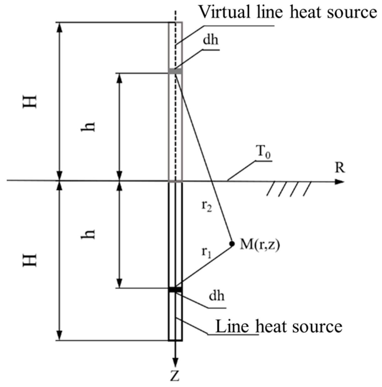
Research on the heat transfer processes within BTES units is typically divided into two domains: inside the borehole and outside the borehole, with the borehole wall serving as the thermal boundary between them. Within the borehole, the thermal capacity of U-shaped pipes, backfill materials, and other internal components is relatively small compared to that of the surrounding soil. As a result, the borehole interior is often assumed to be in a steady-state thermal condition when calculating the fluid temperature. In contrast to the interior of the borehole, heat transfer in the surrounding soil is more complex due to the presence of thermal interactions between adjacent boreholes. Given that the borehole diameter is negligible compared to its depth, the borehole is typically simplified as a finite-length line heat source. This model represents an analytical solution for the temperature of the thermal storage unit, derived by introducing a virtual heat source based on the classical infinite line source theory. As illustrated in Figure 2, the concept of the virtual heat source method involves placing a virtual line heat sink at the mirror-symmetric position of the borehole with respect to the ground surface. This virtual sink has the same length and heat flux magnitude as the real borehole but with an opposite heat flow direction. The superposition of the real and virtual sources ensures that the ground surface temperature remains constant. The model is based on the following assumptions: 1. The initial temperature of the subsurface soil is spatially uniform. 2. The ground surface temperature remains constant and is equal to the initial soil temperature. 3. The subsurface soil is treated as a semi-infinite heat transfer unit. 4.The thermal properties of the soil are homogeneous and temperature-independent. 5.The borehole geometry is neglected, and the borehole is approximated as a finite-length line heat source along its vertical axis.

2.1.1. Single-Point Temperature Prediction

Based on the finite line source model, the temperature response at an arbitrary point induced by a step heat input from a single borehole can be expressed as follows:

$$T(r,z,\tau )-T_0={\displaystyle \frac{q}{4\pi k_s}}{\displaystyle {\int }_0^1[\frac{erfc(\stackrel{~+}{r}/2\sqrt{Fo})}{\stackrel{~+}{r}}-\frac{erfc(\stackrel{~-}{r}/2\sqrt{Fo})}{\stackrel{~-}{r}}]}d\xi$$

(1)

where $\stackrel{~+}{r}=\sqrt{{\beta }^2+{(\eta -\xi )}^2}$; $\stackrel{~-}{r}=\sqrt{{\beta }^2+{(\eta +\xi )}^2}$; η = z/H (relative depth); β = r/H (relative distance); ξ = h/H (relative vertical distance); Fo = ατ/H² (Fourier number); q is the heat injection rate per unit length of the borehole; H is the borehole depth; k_s is the thermal conductivity of the soil; α is the thermal diffusivity of the soil; τ is the time; T₀ is the initial ground temperature.

According to the definition of the g-function proposed by Eskilson [11], the single-borehole g-function for the finite-length line heat source model is expressed as follows:

$$g(\beta ,\eta ,Fo)={\displaystyle \frac{1}{2}}{\displaystyle {\int }_0^1[\frac{erfc(\stackrel{~+}{r}/2\sqrt{Fo})}{\stackrel{~+}{r}}-\frac{erfc(\stackrel{~-}{r}/2\sqrt{Fo})}{\stackrel{~-}{r}}]}d\xi$$

(2)

The temperature at a given point within a borehole field can be determined using the superposition principle, which involves calculating the temperature response of each individual borehole at that point and then summing these responses. Accordingly, the g-function at a given point within a borehole group is expressed as follows:

$$g(\beta ,\eta ,Fo)={\displaystyle \sum _{i=1}^{N}g({\beta }_i,\eta ,Fo)}$$

(3)

Under variable heat flow conditions, the heat flow q can be approximated as a series of rectangular pulse heat flows q(τ_i) (where i = 1, 2, 3, …, n). Each pulse heat flow can be considered as the sum of two step heat flows. Therefore, the temperature response at a specific point at time τ_j, resulting from a pulse heat flow applied during the interval [τ_i−1, τ_i], is given by:

$$T_0={\displaystyle \frac{1}{2\pi k_s}}q({\tau }_i)[g(\beta ,\eta ,F{o}_j-F{o}_{i-1})-g(\beta ,\eta ,F{o}_j-F{o}_i)],(j\ge i)$$

(4)

The dimensionless temperature response function at a specific point, induced by a rectangular pulse heat flow over a time interval Δτ, is defined as follows:

$$f(\beta ,\eta ,Fo)=g(\beta ,\eta ,Fo)-g(\beta ,\eta ,Fo-\mathrm{\Delta }Fo)={\displaystyle \underset{0}{\overset{\mathrm{\Delta }Fo}{\int }}{g}^{\prime }(\beta ,\eta ,Fo-\tau )}d\tau$$

(5)

where ΔFo = α·Δτ/H² denotes the Fourier number interval.

Therefore, the temperature response at time τ_j can be determined using the superposition principle, by calculating the temperature response of each pulse heat flow segment and subsequently summing these contributions:

$$T_{\mathrm{j}}-T_0={\displaystyle \frac{1}{2\pi k_s}}{\displaystyle \sum _{i=1}^{j}q({\tau }_i)f(\beta ,\eta ,F{o}_j-F{o}_{i-1})}$$

(6)

2.1.2. Average Temperature Prediction

According to the finite line heat source model, determining the average temperature of the thermal storage unit is equivalent to evaluating the dimensionless temperature response of the heat input over the entire volume. Once the dimensionless temperature response at a single point is established, the overall response can be obtained by performing a volume-averaged integral. According to Equations (5) and (6), the key to determining the average temperature of the thermal storage unit lies in calculating the partial derivative G′ of the storage unit’s G-function with respect to the Fourier number, as well as the corresponding value of F.

As illustrated in Figure 1, a rectangular coordinate system is established with the center of the buried pipe as the origin. The relative distances x₁, x₂, y₁, and y₂ from the pipe center to the boundaries of the thermal storage unit are determined to define the integration domain. Neglecting the influence of the borehole, the derivative of the G-function for the thermal storage unit, G, is calculated as follows:

$$\begin{array}{cc}\hfill G^{\prime }& ={\displaystyle \frac{1}{lw}}{\displaystyle \underset{0}{\overset{1}{\int }}{\displaystyle \underset{y_1}{\overset{y_2}{\int }}{\displaystyle \underset{x_1}{\overset{x_2}{\int }}{g}^{\prime }dxdyd\eta }}}\hfill \\ \hfill & ={\displaystyle \frac{1}{lw}}{\displaystyle \underset{y_1}{\overset{y_2}{\int }}{\displaystyle \underset{x_1}{\overset{x_2}{\int }}\frac{\exp ((-x^2-y^2)/4Fo)}{4Fo}(2-4erfc(\frac{1}{2\sqrt{Fo}})+2erfc(\frac{1}{\sqrt{Fo}})-A(Fo))dxdy}}\hfill \end{array}$$

(7)

where l = L/H; w = W/H; A$= 2\sqrt{Fo}\left(\right(exp\left(-1/Fo\right)-4exp\left(-1/4Fo\right)+ 3\left)\right)/\sqrt{\mathsf{\pi }}$; W and L represent the width and length of the thermal storage unit, respectively.

Let B$\left(Fo\right) = 2-4erfc\left(1/2\sqrt{Fo}\right) + 2erfc\left(1/\sqrt{Fo}\right)-\mathrm{A}\left(Fo\right)$. Further derivation then yields:

$$G^{\prime }={\displaystyle \frac{\pi B(Fo)}{4lw}}(erf({\displaystyle \frac{x_2}{2\sqrt{Fo}}})-erf({\displaystyle \frac{x_1}{2\sqrt{Fo}}}))(erf({\displaystyle \frac{y_2}{2\sqrt{Fo}}})-erf({\displaystyle \frac{y_1}{2\sqrt{Fo}}}))$$

(8)

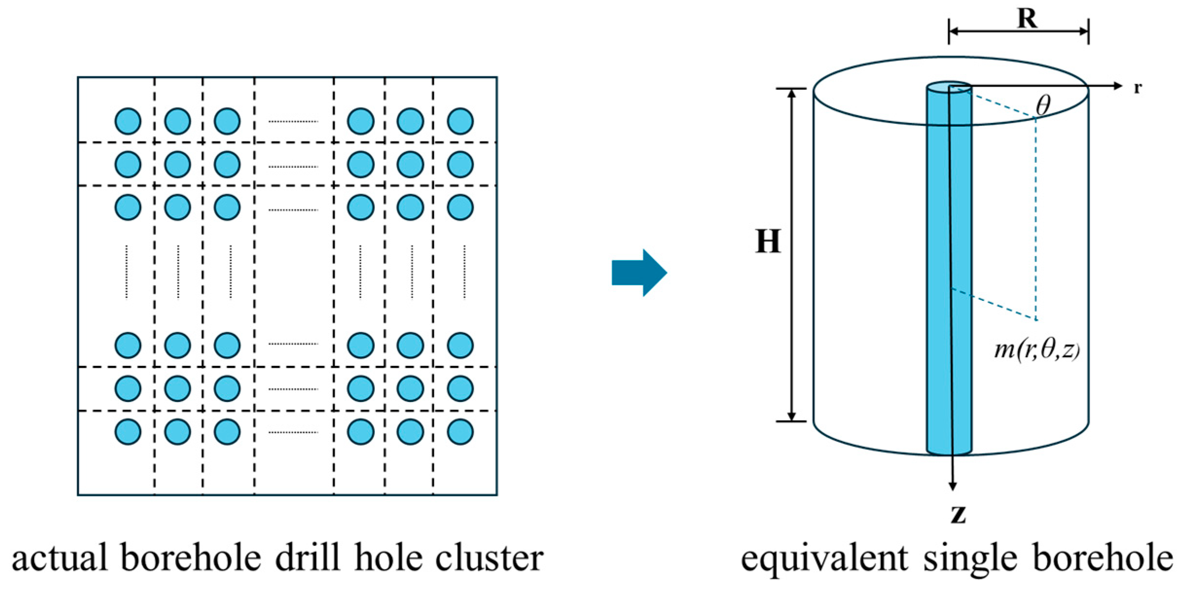
By combining Equations (6) and (8), a thermal response model for the heat flow from a single pipe to the heat storage unit can be established. Owing to the symmetrical arrangement of the buried pipes, it is sufficient to calculate only one-eighth of the domain to obtain the overall temperature response. To address the computational complexity introduced by the large number of buried pipes in practical engineering applications, this study further proposes an equivalent single-pipe model. In this model, the distributed heat sources are represented by a single, centralized line heat source located at the center of a cylindrical heat storage unit, while preserving the total heat input and geometric volume.

Figure 3 illustrates the geometric configuration of the equivalent single-borehole heat storage unit. Similarly to the procedure used for rectangular heat storage bodies, the volume-averaged integral of the G function with respect to the Fourier number (Fo) must be evaluated to obtain its partial derivative, G′.

Following the derivation process of Equation (7), the expression for G′ in the equivalent single-borehole model is given as follows:

$$\begin{array}{cc}\hfill G^{\prime }& ={\displaystyle \frac{1}{\pi r^2}}{\displaystyle \underset{0}{\overset{1}{\int }}{\displaystyle \underset{0}{\overset{2\pi }{\int }}{\displaystyle \underset{0}{\overset{r}{\int }}{g}^{\prime }rdrd\theta d\eta }}}\hfill \\ \hfill & ={\displaystyle \frac{B(Fo)}{\pi r^2}}{\displaystyle \underset{0}{\overset{2\pi }{\int }}{\displaystyle \underset{0}{\overset{r}{\int }}\frac{\exp (-r^2/4Fo)}{4Fo}}}rdrd\theta ={\displaystyle \frac{B(Fo)}{r^2}}(1-\exp (-r^2/4Fo))\hfill \end{array}$$

(9)

where r = R/H represents the dimensionless radius of the equivalent single-borehole heat storage unit.

2.1.3. Heat Transfer Within Boreholes

In the context of heat transfer within boreholes, the temperature of the fluid is the most critical parameter from an engineering perspective. Due to the relatively small structural dimensions and low thermal capacity of borehole components, as well as the slow temporal variation in temperature, the heat transfer process is typically simplified as steady-state. This assumption has been validated as reasonable in long-term thermal simulations of buried pipe systems [14].

Zeng et al. [17,18,19] accounted for the variation in fluid temperature with depth while neglecting axial heat conduction within the borehole, and thereby established a quasi-three-dimensional steady-state heat transfer model. Based on this model, the fluid temperature within the borehole can be calculated using the following equation:

$$\begin{array}{c}{\mathrm{\Theta }}_d(Z)=\mathrm{ch}(\beta Z)-{\displaystyle \frac{1}{\beta S_{12}}}\left[({\displaystyle \frac{S_{12}}{S_1}}+1)-{\displaystyle \frac{\beta S_1\cdot \mathrm{ch}\beta -\mathrm{sh}\beta }{\beta S_1·\mathrm{ch}\beta +\mathrm{sh}\beta }}\right]\mathrm{sh}(\beta Z)\\ {\mathrm{\Theta }}_u(Z)={\displaystyle \frac{\beta S_1·\mathrm{ch}\beta -\mathrm{sh}\beta }{\beta S_1·\mathrm{ch}\beta +\mathrm{sh}\beta }}\mathrm{ch}(\beta Z)-{\displaystyle \frac{1}{\beta S_{12}}}\left[1-({\displaystyle \frac{S_{12}}{S_1}}+1)-{\displaystyle \frac{\beta S_1\cdot \mathrm{ch}\beta -\mathrm{sh}\beta }{\beta S_1\cdot \mathrm{ch}\beta +\mathrm{sh}\beta }}\right]\mathrm{sh}(\beta Z)\end{array}$$

(10)

where Z is the dimensionless depth parameter of the U-tube, defined as Z = z/H, where z is the vertical coordinate ranging from 0 to H; ${\mathrm{\Theta }}_d$ and ${\mathrm{\Theta }}_u$ represent the temperatures of the downward- and upward-flowing fluid in the vertical U-tube, respectively, ${\mathrm{\Theta }}_d=(T_d-T_b)/(T_{in}-T_b)$, ${\mathrm{\Theta }}_u=(T_u-T_b)/(T_{in}-T_b)$; T_b denotes the borehole wall temperature; T_d and T_u represent the temperatures of the downward- and upward-flowing fluid in the vertical U-tube, respectively; $\beta =\sqrt{1/S_1^2+2/(S_1{S}_{12})}$; S₁ and S₁₂ refer to the dimensionless thermal resistances between the fluid and the borehole wall, and between fluids in adjacent U-tube legs, respectively. The detailed calculation methods for these parameters can be found in [14].

Then, the dimensionless outlet temperature of the fluid can be expressed as follows:

$${\mathrm{\Theta }}_{out}={\mathrm{\Theta }}_u(0)={\displaystyle \frac{\beta S_1·\mathrm{ch}\beta -sh\beta }{\beta S_1·\mathrm{ch}\beta +sh\beta }}$$

(11)

2.2. Temperature Distribution Calculation Method Based on Two-Dimensional Discrete Convolution

In simulation analyses, the temperature distribution within the thermal storage unit represents a key area of investigation. Due to the temperature superposition effect among boreholes, large-scale temperature field calculations become computationally intensive. As a result, most existing studies are limited to systems with fewer than 300 boreholes. To address this challenge, the concept of thermal influence distance has been introduced [20], allowing calculations to be restricted to boreholes within a defined influence range, as the thermal impact of distant boreholes is relatively negligible. By first calculating the temperature distribution within the thermal influence zone of a single borehole and then nesting and superimposing this distribution across all boreholes, the complex process of point-by-point computation can be effectively replaced.

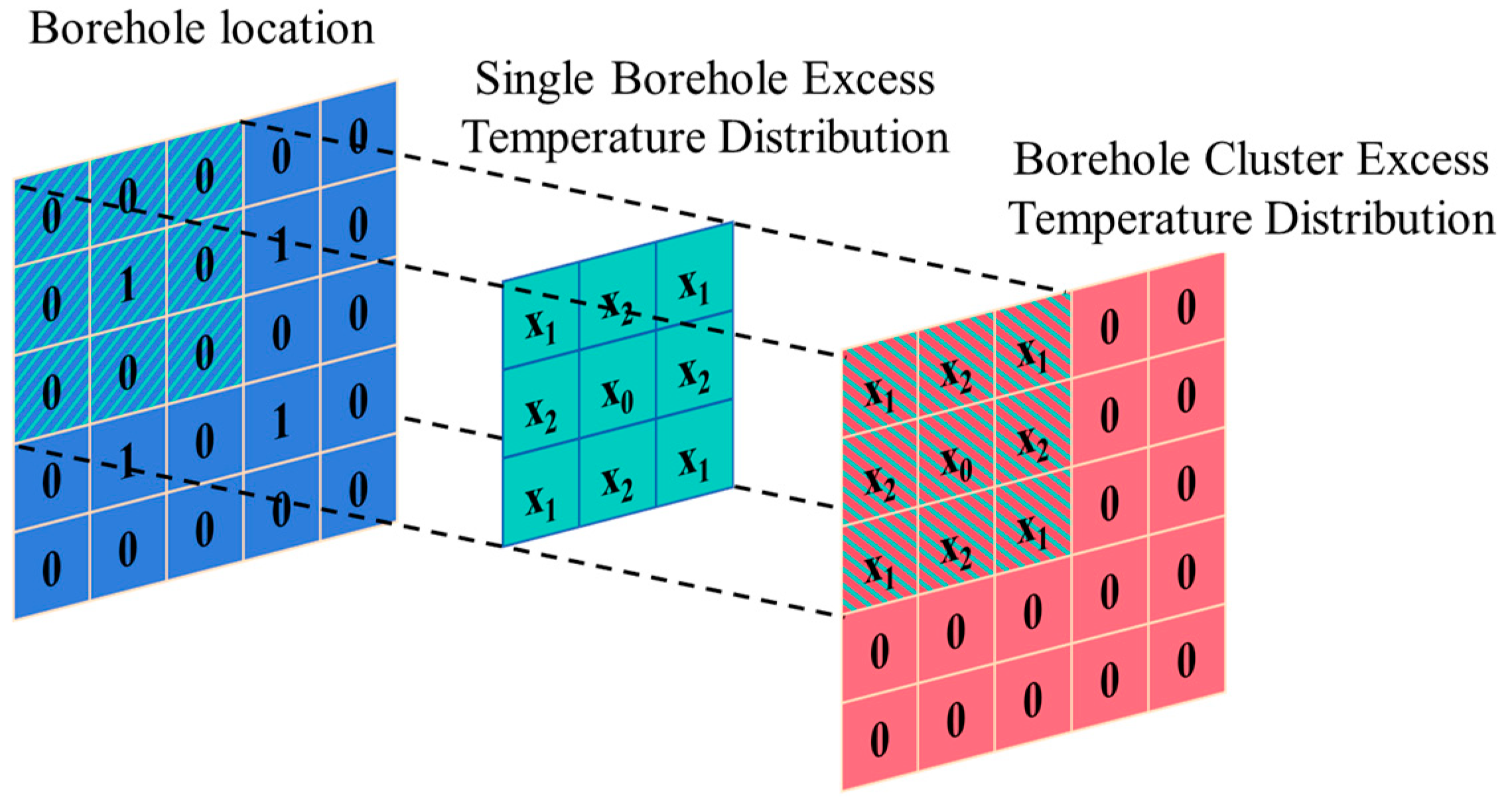
In Figure 4, the borehole location matrix is defined using binary values, where 1 denotes a borehole location and 0 represents soil. The excess temperature distribution for a single borehole is denoted as x_i, with x₀ corresponding to the temperature at the borehole wall. By shifting the single-borehole temperature distribution matrix and aligning its center with each borehole location, the excess temperatures in overlapping regions are progressively nested and summed, thereby constructing the overall temperature distribution. Based on this principle, this study proposes a temperature superposition method using two-dimensional discrete convolution:

$$C(i,j)={\displaystyle \sum _m{\displaystyle \sum _{n}A(m,n)B(i-m,j-n)}}$$

(12)

where A, B, and C represent the input layer, kernel, and output layer, respectively.

Two-dimensional discrete convolution produces the output layer C by sliding the convolution kernel B across the input layer A, performing element-wise multiplication, and summing the results. There are three common convolution modes—FULL, VALID, and SAME—which correspond to different traversal strategies and output dimensions. In this study, the SAME mode is employed to ensure that the output layer maintains the same size as the input layer, thereby satisfying the dimensional requirements of the calculation. When solving temperature fields of non-uniformly spaced borehole groups using two-dimensional discrete convolution, the borehole spacing must satisfy the commensurability condition: there must exist a common measure length Δ such that all physical spacings are integer multiples of Δ. This Δ then serves as the spatial step size for discrete grids, enabling the construction of position matrices. Consider four non-uniformly arranged boreholes with successive spacings of 1 m, 3 m, and 3.5 m as an example. Here, Δ = 0.5 m may be selected as the unified discretization step. Borehole nodes are subsequently assigned values of 1 in the position matrix, while 2, 6, and 7 zero-value nodes representing soil are sequentially inserted between adjacent boreholes. This procedure achieves the regular grid mapping required for convolutional operations. For completely random borehole arrangements violating the commensurability condition, one must revert to a stepwise superposition method. Temperature responses are then calculated by progressively superimposing pairwise temperature fields.

In SAME mode, the center of the convolution kernel traverses every position within the input layer. As illustrated in Figure 5, the input layer corresponds to the borehole location matrix, the convolution kernel (with odd dimensions) represents the temperature distribution of a single borehole, and the output layer yields the residual temperature distribution of the entire borehole group. Due to the symmetrical nature of the single borehole temperature distribution, the convolution operation becomes equivalent to a cross-correlation, meaning that flipping the kernel has no effect on the outcome. Throughout the traversal process, a stride of 1 is used. When the kernel extends beyond the input boundaries, zero-padding is applied to the input layer (indicated by the gray regions in Figure 5) to ensure that a complete output of consistent size is generated.

As shown in Figure 5, when the input layer region corresponding to the convolution kernel contains 1, it indicates that the position is affected by borehole heat. After calculation, only the positions with a value of 1 in the input layer generate excess temperature, while positions with a value of 0 have no heat contribution. The calculation results are assigned to the corresponding output layer positions. When the convolution kernel covers multiple drill holes, the thermal effects of multiple drill holes are automatically superimposed, making the two-dimensional discrete convolution results completely consistent with the direct nesting method. Let the drill hole position matrix be n × n, the number of drill holes be m × m, and the convolution kernel be k × k. Then, the computational complexity of the direct nesting method is O(m²k²), and that of the two-dimensional discrete convolution is O(n²k²). Although the two-dimensional discrete convolution has slightly increased computational complexity, it can significantly improve computational efficiency through parallel processing, fast Fourier transforms, and other techniques. Therefore, this method is more advantageous for handling large-scale data and provides a reliable solution for calculating the temperature distribution of large-scale borehole clusters.

2.3. Convolution Algorithm Based on Fast Fourier Transform

When dealing with long time scales and small time steps, the volume of data associated with heat flux and thermal response factors becomes substantial, resulting in a significant slowdown in computational efficiency. To address this issue, Denis [21] introduced the use of the discrete Fourier transform (DFT) and its fast implementation, the fast Fourier transform (FFT), to accelerate convolution calculations. According to the convolution theorem, the DFT of the convolution of two sequences is equal to the element-wise product of their respective DFTs. For two sequences x(n) and h(n) each of length N, their convolution y(n) = x(n) * h(n) can be computed through the following steps:

• Discrete Fourier Transform: Calculate the DFT of x(n) and h(n) to obtain their frequency-domain representations X(k) and H(k), respectively.

  $$X(k)={\displaystyle \sum _{n=0}^{N-1}x(n)}\cdot e^{-j2\pi kn/N}$$

  (13)

  $$H(k)={\displaystyle \sum _{n=0}^{N-1}h(n)\cdot e^{-j2\pi kn/N}}$$

  (14)
• Product: Compute the element-wise product of X(k) and H(k) to obtain Y(k), the frequency-domain representation of the convolution result.

  $$y(n)={\displaystyle \frac{1}{N}}{\displaystyle \sum _{k=0}^{N-1}Y(k)}\cdot e^{j2\pi kn/N}$$

  (15)
• Inverse DFT: Perform the inverse DFT on Y(k) to obtain y(n), the final convolution result in the time domain.

  $$y(n)={\displaystyle \frac{1}{N}}{\displaystyle \sum _{k=0}^{N-1}Y(k)}\cdot e^{j2\pi kn/N}$$

  (16)

The FFT algorithm enables both the DFT and its inverse to be computed in O(NlogN) time. As a result, the overall computational complexity of convolution operations is reduced to O(NlogN), which is significantly more efficient than the O(N²) complexity associated with direct convolution methods.

Since Equation (6) represents a linear convolution, modifications are necessary to adapt the FFT—which inherently performs cyclic convolution—for linear convolution computations. To meet the requirements of linear convolution, both the sequence q(τ_i) and the index of Fo_i must begin at zero, which involves applying zero-padding and shifting the data one position to the left. Consequently, the index of the temperature sequence T_j should also be adjusted to start from zero.

$$\begin{array}{cc}\hfill T-T_0& ={\displaystyle \frac{1}{2\pi k_s}}{\displaystyle \sum _{i=1}^{j}q({\tau }_i)f(\beta ,F{o}_j-F{o}_{i-1})}\hfill \\ \hfill & ={\displaystyle \frac{1}{2\pi k_s}}{\displaystyle \sum _{i=0}^{j}q({\tau }_i)f(\beta ,F{o}_{j-i})}\hfill \end{array}$$

(17)

Since the effective length of the sequence is j, the heat flow sequence q(τ_i) and the thermal response factor sequence f(β,Fo_i) are defined as zero when i < 0 or i ≥ j. Under this condition, Equation (17) can be further expressed as:

$$T-T_0={\displaystyle \frac{1}{2\pi k_s}}{\displaystyle \sum _{i=-\infty }^{+\infty }q({\tau }_i)f(\beta ,F{o}_{j-i})}$$

(18)

Therefore, to satisfy the conditions for linear convolution, both q(τ_i) and f(β,Fo_i) must undergo a (2j − 1)-point FFT. After computing the product of the transformed sequences, an inverse FFT is performed, and the first j points of the result are taken as the effective temperature values.

3. Results and Discussion

3.1. Engineering Algorithm for Single-Point Temperature Calculation

In the theory of finite-length line heat sources, the calculation of the g-function and the f-function involves error functions and complex integral operations, which considerably increase the computational burden when determining the temperature of the thermal storage unit. To address this issue, this study conducted an in-depth analysis of the variation pattern of f(β,η,Fo_j − Fo_i−1) (hereinafter referred to as the f-value) and developed a simplified, engineering-oriented algorithm using the MATLAB Curve Fitting Toolbox.

To obtain an engineering algorithm with broad applicability, this study systematically investigated the variation characteristics of the f-value under different parameter conditions. The reference values for each variable were set as follows: pipe length H = 150 m, thermal diffusivity α = 4.79 × 10⁻⁷ m²/s, relative distance β = 0.01, and relative depth η = 0.5. Based on these parameters, each variable was adjusted individually to obtain the time-dependent variation in the f value (with a calculation time interval of 1 h), as shown in Figure 6. Figure 6a,b illustrate the influence of different heat storage unit design parameters and material properties on the variation in the f value, while Figure 6c,d show the variation characteristics of the f value under different relative distance and relative depth conditions.

Over time, the f-values exhibit a characteristic trend of initially increasing and then decreasing, resembling an asymmetric Gaussian function. This pattern reflects the time-dependent nature of heat transfer in the borehole, where the influence of a heat pulse at a given point is delayed due to the finite speed of thermal diffusion. As heat requires time to propagate, the f values consistently follow this rise-and-fall behavior. Furthermore, increases in borehole depth, reductions in thermal diffusivity, or greater spatial separation result in a significant delay before a monitoring point responds to a given heat input. Further analysis reveals that the maximum value of f, denoted f_max, and its corresponding time t_cen, exhibit clear functional relationships with the borehole length H, thermal diffusivity α, and dimensionless relative distance β. In Figure 6a, as the borehole length H increases from 100 m to 150 m, f_max decreases from 0.001270 to 0.000564—approximately a 2.25-fold reduction—while t_cen increases from 145 h to 325 h, a 2.25-fold increase. These trends indicate that f_max is proportional to 1/H² and t_cen is proportional to H². In Figure 6b, as the thermal diffusivity α increases from 2.395 × 10⁻⁷ m²/s to 4.79 × 10⁻⁷ m²/s, f_max roughly doubles and t_cen is halved, indicating that f_max ∝ α, and t_cen ∝ 1/α. In Figure 6c, as the relative distance β increases from 0.01 to 0.03, f_max decreases to approximately one-ninth of its original value, while t_cen increases by a factor of 9, suggesting that f_max ∝ 1/β² and t_cen ∝ β². However, Figure 6d shows that f_max and t_cen do not follow consistent patterns with changes in relative depth. This deviation is primarily attributed to boundary effects at the top and bottom of the borehole. Within the finite-length line heat source model, the upper boundary is typically modeled as a constant-temperature surface, while the lower boundary facilitates more efficient heat dissipation compared to the borehole’s central section, thereby disrupting the symmetry observed in other parameter variations.

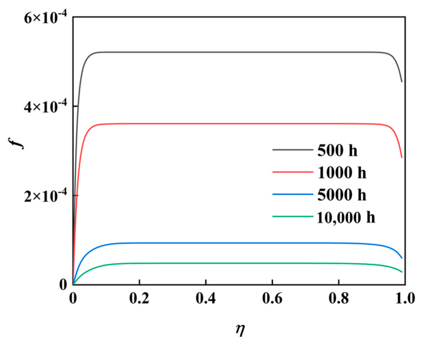
Figure 7 illustrates the temporal variation in the f-value at different normalized depth positions. The analysis indicates that when the dimensionless depth η ranges from 0.1 to 0.9, the variation profiles of f-values remain consistent and stable across different positions. However, in the regions near the top and bottom boundaries (i.e., η approaching 0 or 1), significant deviations occur, primarily due to boundary effects. These deviations arise from the constant-temperature condition imposed at the borehole top and the enhanced heat dissipation at the bottom boundary, which alter the thermal response compared to the borehole’s central region. Recognizing this behavior, the present study selects the f-value at the mid-depth position (η = 0.5) as the baseline for function fitting. The variation in f-values at other depth positions is then characterized by their ratio relative to this reference curve, enabling a simplified yet accurate representation of depth-dependent thermal response patterns.

Combining the observations from Figure 6 and Figure 7, it can be concluded that for η = 0.5, the maximum value f_max and the corresponding time t_cen can be estimated using the following equations:

$$f_{\max }={\displaystyle \frac{\alpha }{3.744\times {10}^{-4}{H}^2{\beta }^2}}$$

(19)

$$t_{cen}={\displaystyle \frac{6.946\times {10}^{-5}{H}^2{\beta }^2}{\alpha }}$$

(20)

Since the f-value exhibits an asymmetric Gaussian-like shape resembling an “S” curve, it was decided to fit the segments before and after the time point t_cen separately. The initial ascending portion of the curve was fitted using a Sigmoid function, while the descending segment was fitted with an inverse proportional function. This fitting approach yields the following expression for the f value:

$$f_{fit}=\left\{\begin{array}{cc}{\displaystyle \frac{n}{4.7354t_{cen}(1+\exp (-10t/t_{cen}+4))}},& t<t_{cen}\\ {\displaystyle \frac{n}{2t+2.736t_{cen}}},& t\ge t_{cen}\end{array}\right.$$

(21)

$$n={\displaystyle \frac{2}{1+\exp (\frac{-\eta {\alpha }^{-0.5}H}{14.946t^{0.6}+1169.487})}}-{\displaystyle \frac{2}{1+\exp (\frac{-\eta +20.72t^{0.6}+1.005{\alpha }^{-0.5}H}{19.148t^{0.6}+992.2})}}-1$$

(22)

where t denotes the cumulative time in hours, and n represents the ratio of the f_η-value at a given depth to the reference value at η = 0.5 at the same time.

3.2. Engineering Algorithm for Average Temperature Calculation

To evaluate the applicability of the equivalent single-borehole model, this study employs a characteristic borehole cluster model for comparative analysis. Its principle is shown in Figure 8.This model is founded on the principle that, within a certain time frame, due to the limited range of thermal influence [20], the soil temperature surrounding a single borehole is primarily affected by the heat flow of the borehole itself and its adjacent boreholes. Based on this premise, a representative characteristic borehole cluster can be identified [22]. By calculating the average soil temperature around each borehole under the thermal influence of the characteristic cluster, and then mapping this average soil temperature to the actual borehole field, the temperature distribution can be effectively predicted. The computational procedure of this method is based on Equation (8).

Based on the single-borehole load model presented in Reference [21], the annual heat flux per meter of a single borehole can be determined, enabling an estimation of the temperature influence range of the buried pipe. The specific calculation formula is as follows:

$$q(\tau )=A-B\cos ({\displaystyle \frac{\tau }{8760}}2\pi )-C\cos ({\displaystyle \frac{\tau }{24}}2\pi )-D\cos ({\displaystyle \frac{\tau }{24}}2\pi )\cos ({\displaystyle \frac{2\tau }{8760}}2\pi )$$

(23)

where τ denotes time; A represents the annual average load; B is the amplitude of the annual load variation; and C and D represent the amplitude of the daily load variation.

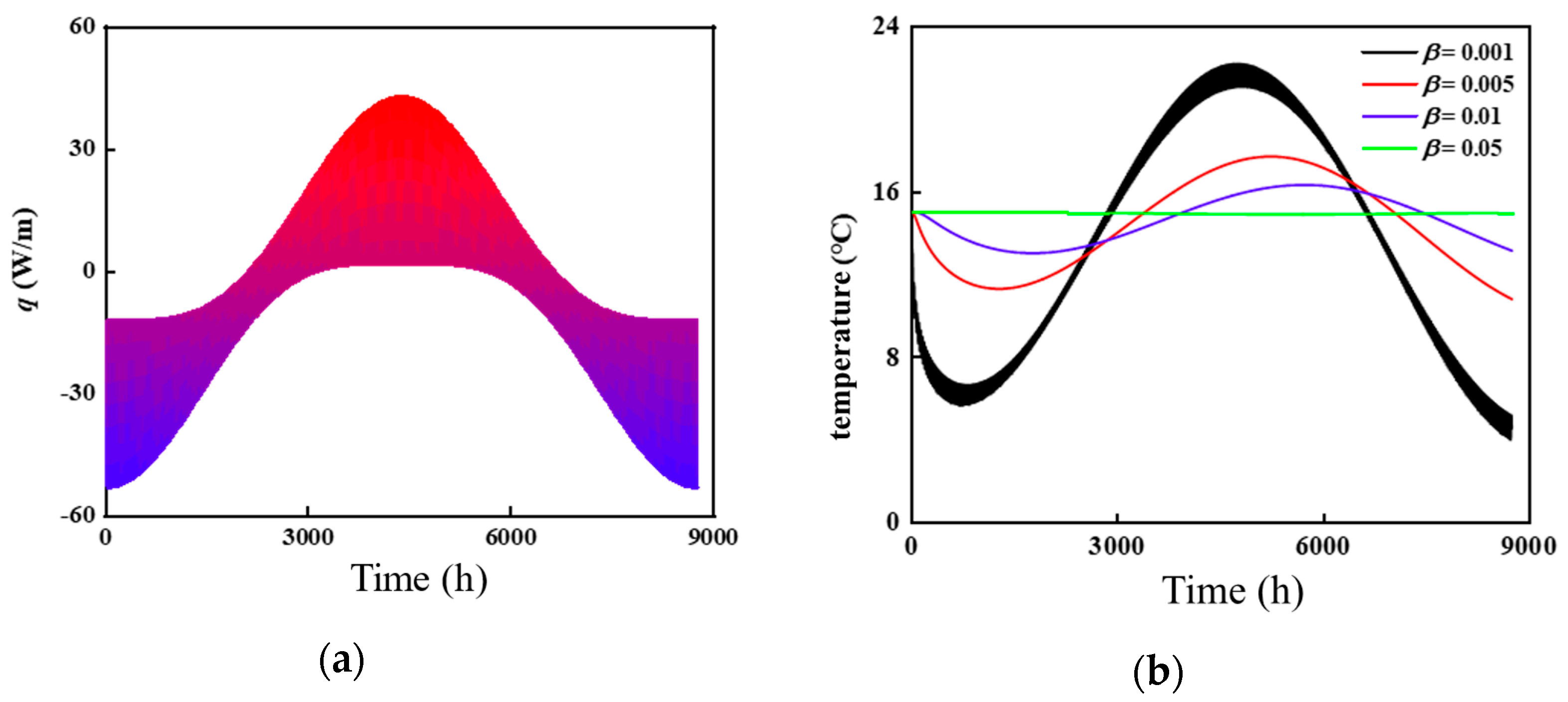
Taking the geological conditions of a specific region as an example [23], the thermal conductivity is k = 1.31 W/(m·K), the thermal diffusivity is α = 4.79 × 10⁻⁷ m²/s, the borehole depth is 150 m, and the spacing between boreholes is 3.3 m. Monitoring points located at a depth of 75 m were selected to study four locations with relative distances β of 0.001, 0.005, 0.01, and 0.05. The annual variation in heat flux per meter along the borehole is shown in Figure 9a, where the maximum summer heat flux reaches 42.3 W/m, and the maximum winter heat flux reaches −53.2 W/m. The corresponding temperature responses at each monitoring point are illustrated in Figure 9b. The results indicate that when β = 0.05, the temperature remains essentially stable, showing no significant variation. Therefore, the effective influence range of the heat flow is determined to be β ≤ 0.05. Based on this influence range, the representative borehole cluster is defined as a 5 × 5 borehole array.

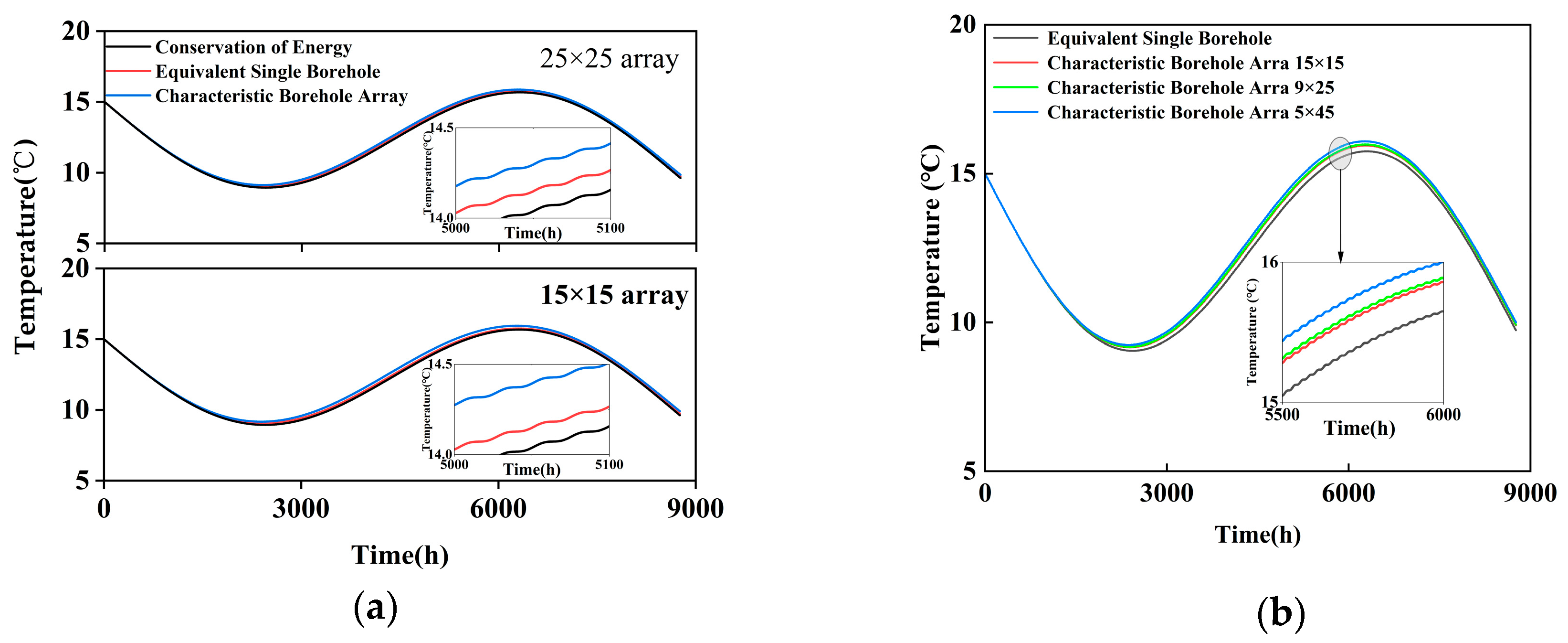
Figure 10a presents a comparison of the two calculation methods under different thermal storage unit scales. For configurations of 15 × 15 and 25 × 25 borehole arrays, the maximum temperature differences between the two methods were 0.25 °C and 0.15 °C, respectively, with corresponding maximum relative errors of 2.0% and 1.2%. The equivalent single-borehole method simplifies rectangular storage bodies into cylindrical ones, which reduces the surface area and thus affects the calculation of the average storage temperature. The volume-to-surface area ratios for the 15 × 15 and 25 × 25 configurations were 0.095 m²/m³ and 0.062 m²/m³, respectively, which changed to 0.084 m²/m³ and 0.056 m²/m³ after applying the equivalent single-borehole simplification, resulting in decreases of 0.011 m²/m³ and 0.006 m²/m³. As the scale of the thermal storage unit increases, the change in volume-to-surface area ratio becomes smaller, and consequently, the discrepancy between the two methods narrows. This phenomenon can be physically attributed to the diminishing influence of boundary heat dissipation on the overall heat transfer process as the storage scale increases. As a result, the outcomes of both methods converge toward the theoretical values derived from the energy conservation equation, demonstrating improved agreement.

Different borehole arrangements also lead to variations in the volume-to-surface area ratio of the thermal storage unit. This study compared three representative configurations: 15 × 15 (square arrangement), 9 × 25 (rectangular arrangement), and 5 × 45 (strip-shaped arrangement). The calculation results are presented in Figure 10b. The corresponding changes in the volume-to-surface area ratio for these configurations were −0.011 m²/m³, −0.021 m²/m³, and −0.064 m²/m³, respectively. The maximum temperature differences in average storage temperature between the two methods were 0.25 °C, 0.28 °C, and 0.42 °C, with associated maximum relative errors of 2.1%, 2.3%, and 3.5%, respectively. The analysis indicates that the closer the borehole arrangement is to a square geometry, the higher the accuracy of the equivalent single-borehole model and the smaller the resulting computational error. This is because the equivalent single-borehole model achieves higher accuracy in square borehole arrays (e.g., 15 × 15) compared to rectangular or strip-shaped configurations (e.g., 5 × 45). This discrepancy primarily stems from the coupled effects of geometric asymmetry and enhanced boundary dissipation. Geometrically, strip-shaped layouts exhibit a lower surface-area-to-volume ratio, resulting in greater heat dissipation per unit volume. Regarding boundary conditions, such configurations possess a higher proportion of boreholes near domain edges, where accelerated lateral heat flux amplifies deviations in mean temperature predictions. In contrast, square arrays align more closely geometrically with the symmetric cylindrical equivalence model, thereby mitigating boundary dissipation effects and improving predictive accuracy. Consequently, the suboptimal performance of elongated regular configurations arises fundamentally from the synergistic interaction of geometric asymmetry and boundary-enhanced heat dissipation.

The following section derives the engineering algorithm for the equivalent single-borehole method by combining it with Equation (7), focusing on the relationship between the F-value of the heat storage unit and various influencing parameters. The initial parameter values used in the analysis are: borehole depth H = 150 m, thermal diffusivity α = 4.79 × 10⁻⁷ m²/s, and equivalent radius r = 0.02 m. The corresponding calculation results are presented in Figure 11.

The function trend shown in Figure 11 resembles that of an inverse proportional function. However, as the pipe length H and the relative radius r increase, and the thermal diffusivity α decreases, the variation in the F-value gradually deviates from the typical inverse proportional trend during the initial stage. This phenomenon reflects the underlying mechanism of heat loss affecting the energy balance of the thermal storage unit: with increasing scale and slower heat diffusion, the relative proportion of heat loss in the total energy becomes smaller. Based on this observation, this study adopts a piecewise function to accurately characterize the variation pattern of the F-value. The function’s boundary points are indicated in Figure 11, and the corresponding time values can be estimated using the following equation:

$$t_{mid}={\displaystyle \frac{1.277\times {10}^{-5}{r}^2{H}^2}{\alpha }}$$

(24)

Using the curve fitting toolbox provided by MATLAB 2024a, the engineering algorithm for obtaining the F value is as follows:

$$F_{fit}=\left\{\begin{array}{cc}{\displaystyle \frac{-9.337{\alpha }^{0.5}{t}^{0.5}}{H{t}_{mid}}}+{\displaystyle \frac{0.0919}{t_{mid}}},& t<t_{mid}\\ {\displaystyle \frac{-0.1531r^{0.5}+0.5435}{t+4.334t_{mid}}},& t\ge t_{mid}\end{array}\right.$$

(25)

3.3. Comparison Between Engineering Algorithms and Theoretical Models

To assess the advantages of engineering algorithms over theoretical models in terms of computational efficiency, this section systematically compares and analyzes the computational results obtained from both approaches under various conditions.

Table 1. Comparison of single-point f-value calculations between the theoretical model and engineering algorithm.

H/m	α/(m2/s)	β	η	R2
50	4.79 × 10−7	0.01	0.5	0.994
450	4.79 × 10−7	0.01	0.5	0.991
150	2.395 × 10−7	0.01	0.5	0.994
150	9.58 × 10−7	0.01	0.5	0.995
150	4.79 × 10−7	0.0005	0.5	0.936
150	4.79 × 10−7	0.2	0.5	0.922
150	4.79 × 10−7	0.01	0.05	0.994
150	4.79 × 10−7	0.01	0.95	0.991

and

Table 2. Comparison of F-value calculations for the average temperature between the theoretical model and the engineering algorithm.

H/m	α/(m2/s)	r	R2
50	4.79 × 10−7	0.1	0.983
300	4.79 × 10−7	0.1	0.964
150	2.395 × 10−7	0.1	0.989
150	9.584 × 10−7	0.1	0.989
150	4.79 × 10−7	0.01	0.998
150	4.79 × 10−7	1	0.999

compare the thermal influence factors calculated using the engineering algorithm and the theoretical model under various parameter conditions (assuming a 20-year calculation period with 1 h time intervals). The results show a high degree of consistency between the two approaches. Across the range of investigated variables, the coefficient of determination (R²) consistently exceeds 0.9, clearly demonstrating the high reliability of the engineering algorithm for predicting average temperature. Compared with Equations (5) and (8), the improved formulations—Equations (20) and (23)—effectively eliminate the need for complex functions and integral operations. This simplification significantly reduces computational demands and greatly enhances efficiency, making the engineering algorithm more suitable for practical engineering applications.

To evaluate computational efficiency, the following table compares the execution times of the engineering algorithm and the theoretical model under different simulation durations. All calculations were performed using MATLAB 2024a on a computer with a 2.20 GHz processor. The simulation time spans were set to 1 year, 5 years, and 10 years, with a fixed calculation interval of 1 h. The results are presented in

Table 3. Comparison of computational time for temperature calculations using the engineering algorithm and the theoretical model under different simulation durations.

Time/s		Single-Point Temperature			Average Temperature
		1 year	5 year	10 year	1 year	5 year	10 year
theoretical model	Without FFT	4.612	26.917	77.693	4.761	27.936	80.576
	With FFT	4.380	21.940	44.767	4.740	22.824	46.155
engineering algorithm	Without FFT	0.219	4.988	33.948	0.220	4.993	34.236
	With FFT	0.021	0.092	0.145	0.020	0.081	0.159

. As shown, the engineering algorithm consistently outperforms the theoretical model in terms of computational speed, regardless of whether the FFT technique is applied. Specifically, when the FFT algorithm is used, the computational time for single-point temperature calculations is reduced by approximately 90.4% to 99.9%, while for average temperature calculations, the reduction ranges from 90.9% to 99.9%.

To solve the temperature distribution of the heat storage unit, large-scale datasets such as the borehole position matrix and the convolution kernel are involved. Since a two-dimensional discrete convolution is applied, the FFT can also be used to accelerate the computation. However, the FFT method inherently performs a full convolution (i.e., linear convolution), meaning that convolution operations are computed wherever the input matrix and the kernel intersect. Consequently, the result from the FULL mode does not directly match the output of the SAME mode, which maintains the input matrix dimensions. To address this, the convolution output in FULL mode must be cropped to retrieve the central portion, which corresponds to the output in SAME mode. The acceleration procedure for two-dimensional convolution using FFT follows the same principle as in one-dimensional convolution: both input and kernel matrices are first padded with zeros to accommodate linear convolution, followed by FFT and inverse FFT (IFFT) operations. After the full convolution is computed, the result is cropped to obtain the desired region.

Table 4. Comparison of time required for temperature distribution calculations the temperature distribution calculation using direct two-dimensional convolution and FFT-accelerated convolution.

Input Layer Size	Convolution Kernel Size	Algorithm	Time/s
200 × 200	25 × 25	Without FFT	6.075
		With FFT	0.005
	51 × 51	Without FFT	30.872
		With FFT	0.007
400 × 400	25 × 25	Without FFT	22.141
		With FFT	0.014
	51 × 51	Without FFT	103.507
		With FFT	0.015

presents the computation time comparison for the two-dimensional convolution process, with and without the FFT acceleration algorithm.

As shown in Table 4, the FFT algorithm substantially accelerates the two-dimensional convolution computation, and its efficiency improvement becomes more pronounced as the size of both the input layer and the convolution kernel increases. Specifically, when the input layer is expanded from 200 × 200 to 400 × 400 and the convolution kernel from 25 × 25 to 51 × 51, the computation time with FFT decreases progressively from 8.2‰ to 1.4‰ of that without FFT.

Despite the substantial computational acceleration afforded by FFT, inherent limitations persist. Primarily, FFT exhibits diminishing acceleration returns with excessively large borehole arrays due to prohibitive memory allocation requirements and increased data transfer overhead. Secondly, FFT inherently performs circular convolution, necessitating zero-padding and subsequent truncation to approximate linear convolution operations. While this methodology proves effective for moderate-sized convolution kernels, kernels beyond a critical scale may introduce non-negligible boundary artifacts. Consequently, while FFT-based methods remain computationally viable for most engineering-scale scenarios, applications involving hyper-scale arrays or oversized kernels warrant deliberate evaluation of both memory footprints and perimeter solution fidelity.

3.4. Model Validation

3.4.1. Validation of the Engineering Algorithm for Single-Point Temperature

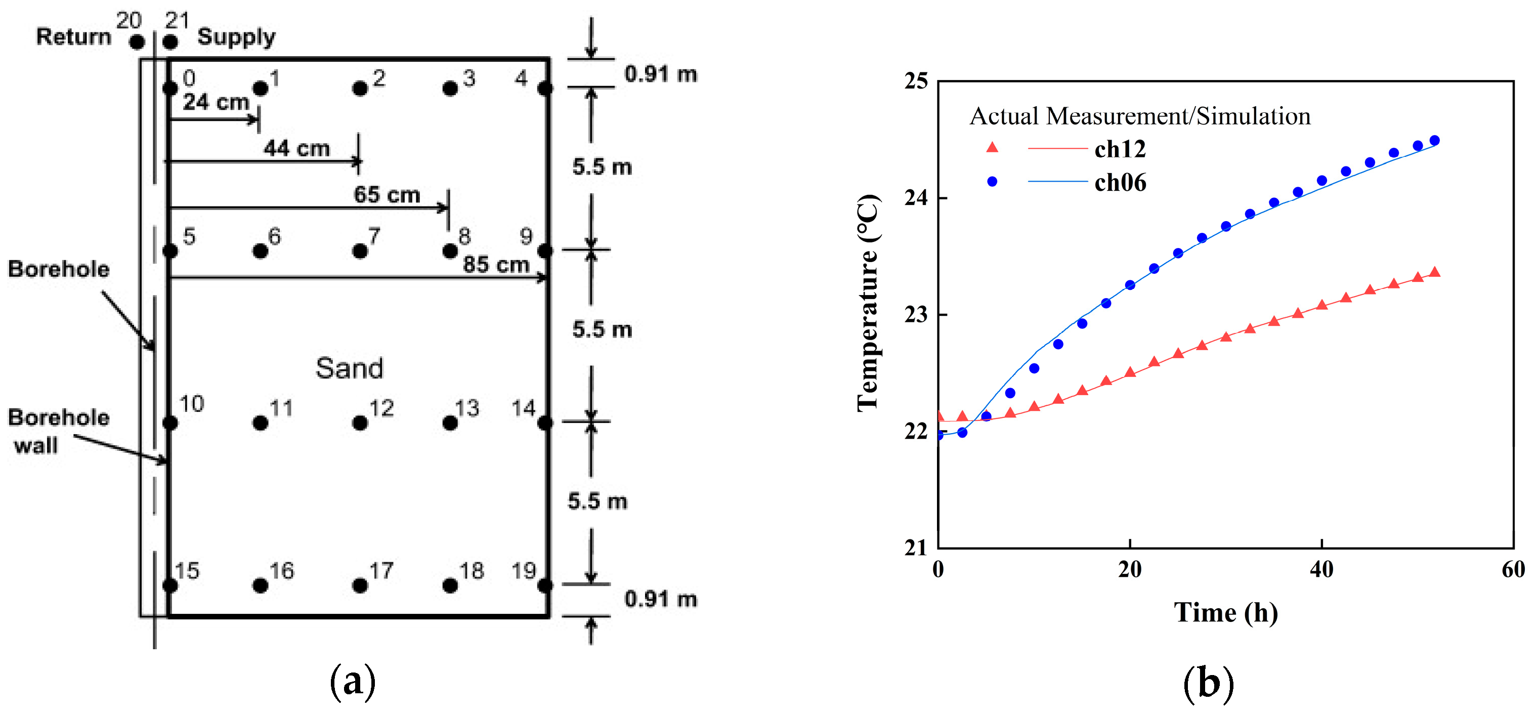
This study validates the single-point temperature engineering algorithm using the sandbox experiment conducted by Beier [24]. In this experiment, a sandbox measuring 1.8 m × 1.8 m × 18.5 m is used to simulate a heat storage unit. An aluminum tube is horizontally embedded at the center of the sandbox to represent a borehole, with a U-shaped water pipe installed inside the aluminum tube. An electric heating device heats the circulating water to mimic the heat transfer process occurring in actual boreholes. The specific parameters of the experimental setup are summarized in

Table 5. Parameters of the Sandbox Experiment [24].

Parameter	Value
Dimensions	1.8 m × 1.8 m × 18.5 m
Aluminum tube diameter	126 mm
Aluminum tube wall thickness	2 mm
U-tube outer (inner) diameter	33.4 (27.3) mm
U-tube length	18.3 m
U-tube thermal conductivity	0.39 W/(m$\cdot$K)
Soil thermal conductivity	2.82 W/(m$\cdot$K)
Backfill material thermal conductivity	0.73 W/(m$\cdot$K)
Sandbox boundary temperature	22 °C
Fluid flow rate	0.197 L/s
Electric heating power	1056 W

.

Figure 12 illustrates the temperature variations at points 06 and 12, as calculated by the single-point temperature engineering algorithm. The results demonstrate a close agreement between the measured and simulated data, with a maximum temperature difference of 0.07 °C and a maximum relative error of 0.3%. This strong correlation between experimental and calculated values confirms the reliability of the single-point temperature engineering algorithm.

3.4.2. Average Temperature Engineering Algorithm Verification

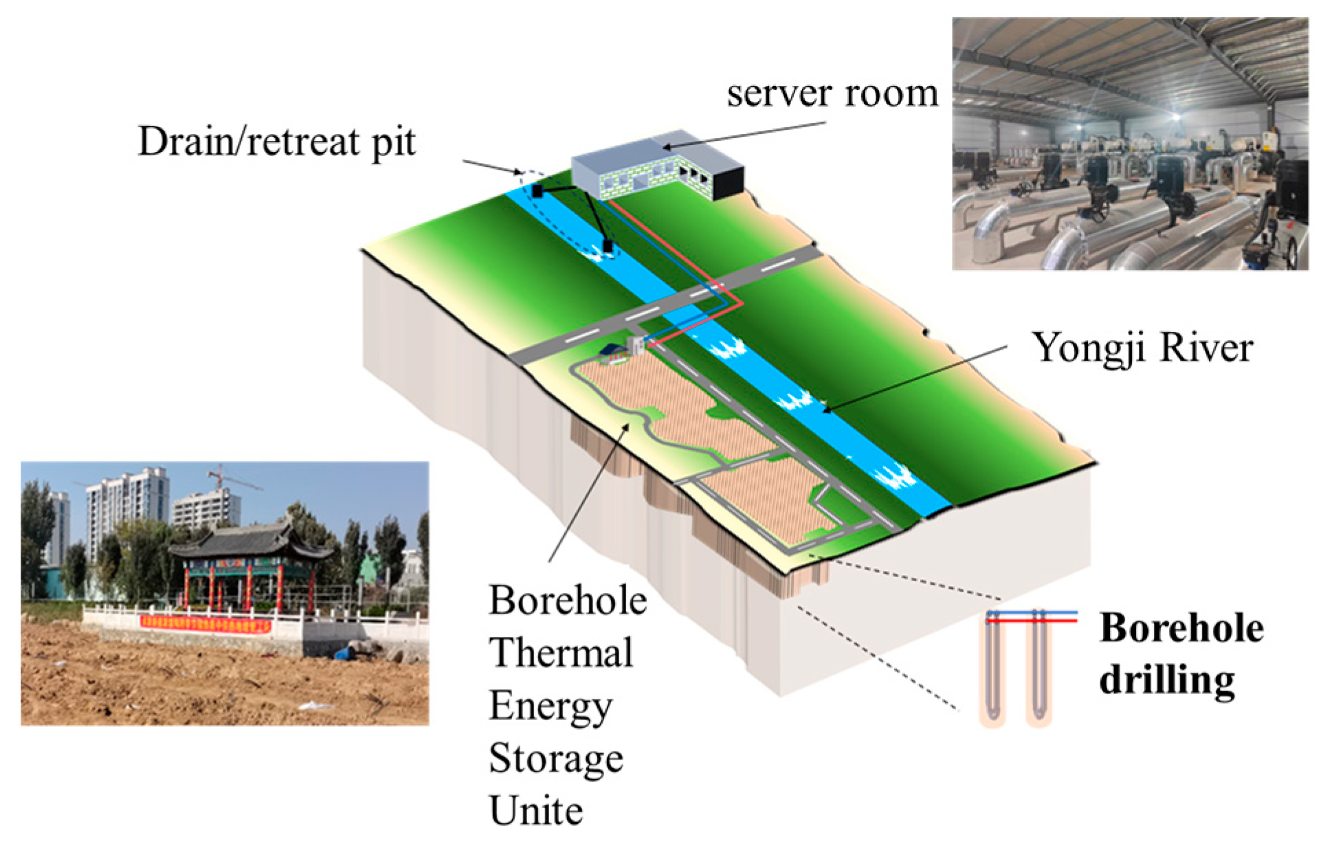
This research validates the outlet temperature of U-tube and the average temperature of the heat storage unit using actual measurement data from the Seasonal BTES project in Guantiao, Hebei Province, China. The project layout is shown in Figure 13. The project comprises 2000 boreholes with a drilling depth of 150 m, resulting in a heat storage unit volume exceeding 3 million m³. The local geological conditions are predominantly clay-based [25], with the following physical properties: thermal conductivity k = 1.31 W/(m·K) and thermal diffusivity α = 6.19 × 10⁻⁷ m²/s. The project was officially commissioned on 15 November 2023, and began experimenting with river water for heat recovery in 2024. For data collection, inlet and outlet temperatures of the units have been automatically recorded hourly since 20 January 2024, when the sensors were installed. Due to the lack of continuous data between 15 November 2023, and 20 January 2024, this study estimates the missing values using measured data from the early part of the 2024 heating season.

Figure 14a shows the variation in inlet and outlet water temperatures of the heat storage unit. Overall, the measured outlet temperature aligns well with the model predictions. However, a larger discrepancy is observed during the later stage of the heat storage period, which may be attributed to missing inlet temperature data during the middle of the storage season. Following the exclusion of anomalous data points, the predictive model exhibited a maximum absolute temperature deviation of 3.6 °C relative to measured values, with a mean error of 0.72 °C (95% CI: 0.674–0.766 °C) and mean relative error of 6%. This discrepancy could be due to manual system adjustments or measurement errors. Since the average temperature of the heat storage unit cannot be directly measured, this study uses the energy system simulation software TRNSYS for validation and comparative analysis. A simulation model was constructed in TRNSYS to match the actual project, ensuring consistency in the number of boreholes, the volume of the heat storage unit, and the inlet conditions of the U-tubes. Figure 14b presents a comparison of the heat storage unit temperature results calculated by the DST model and the proposed engineering algorithm. Given that heat flux data was derived from U-tube inlet/outlet temperature measurements at 1 h intervals, comparative analysis demonstrated strong inter-method agreement with a maximum temperature deviation of 0.19 °C, mean difference of 0.08 °C (95% CI: 0.078–0.082 °C), and maximum relative error of 1.2%, confirming the reliability and accuracy of the engineering algorithm for average thermal storage temperature computation.

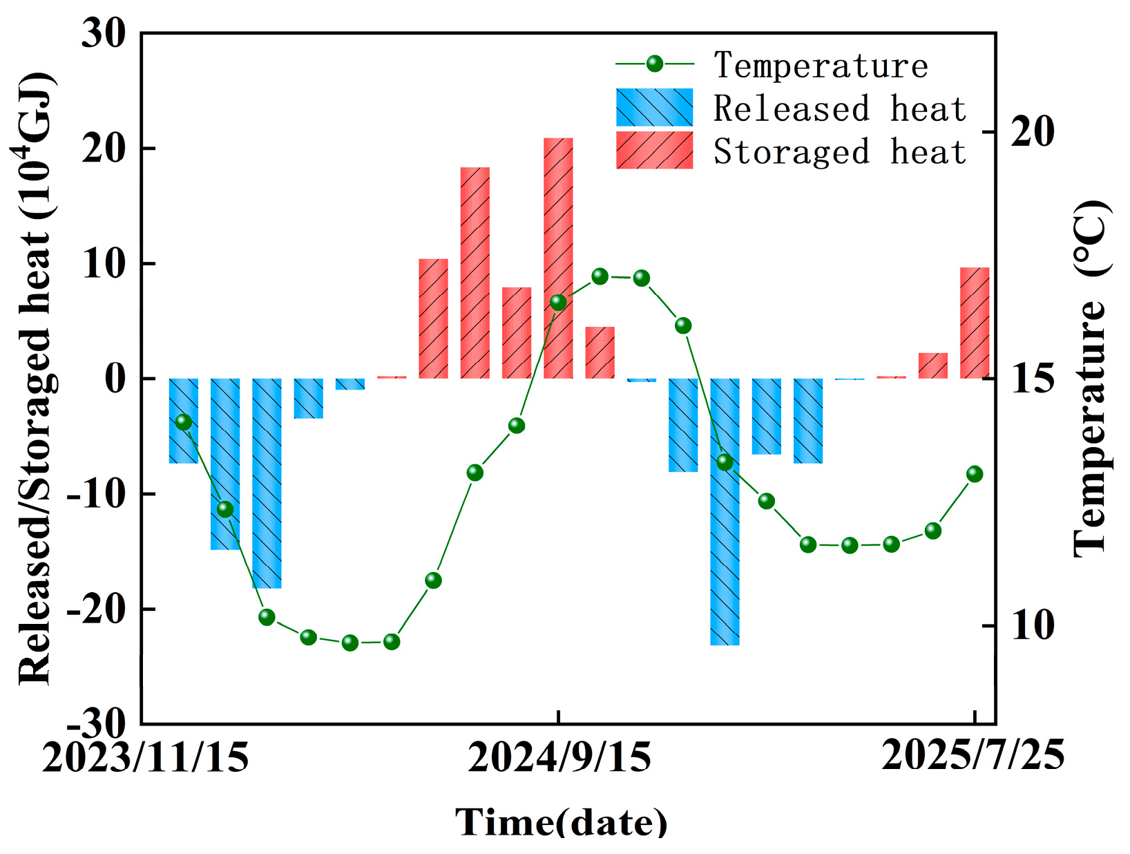
After obtaining the average temperature of the thermal storage unit, the amount of energy stored can be approximately estimated. Figure 15 illustrates the variations in temperature and stored heat of the thermal storage unit since the system commenced operation. As a large-scale BTES system, it is capable of storing and releasing hundreds of thousands of gigajoules (GJ) of heat across seasons. The energy evolution trend indicates that soil heat loss is greatest during the first heating season; however, after a complete heat storage cycle, the temperature of the thermal storage unit in the second heating season is markedly higher than in the first year, leading to a relative decrease in heat loss. Overall, large-scale cross-seasonal ground-coupled thermal storage systems exhibit substantial heat storage capacity and peak-shaving potential, making them an effective technological solution for achieving clean seasonal heating.

4. Conclusions

This study addresses the need for efficient prediction and evaluation of heat storage unit temperatures in STES systems. A rapid calculation framework—free from complex functions and integral operations—is developed at three levels: single-point temperature, average temperature, and temperature distribution. The model is validated using both laboratory experiments and real-world engineering data. The main findings are summarized as follows:

(1)

Single-point temperature prediction: The study explores the variation patterns of thermal influence factors under different parameter conditions. Based on curve-fitting techniques, an engineering-oriented prediction algorithm is proposed that avoids the use of complex functions or integral calculations. Validation against sandbox experimental data shows a maximum temperature deviation of 0.07 °C and a maximum relative error of 0.3%, confirming the algorithm’s high accuracy and practical applicability.

(2)

Average temperature estimation: A theoretical model for the average temperature of the heat storage unit is derived from the finite line source theory. By simplifying the multi-borehole configuration into an equivalent single-borehole cylindrical model, a fast and robust engineering algorithm is developed. Using data from a large-scale cross-seasonal thermal energy storage project in Handan City, Hebei Province, the proposed method demonstrates strong agreement with the established DST (Duct Storage with Pipes) model, with a maximum temperature difference of 0.19 °C and a maximum relative error of 1.2%. These results confirm the model’s reliability and applicability.

(3)

Temperature distribution simulation: To enable efficient modeling of temperature fields in large-scale STES systems, a superposition algorithm based on two-dimensional discrete convolution is introduced. The method limits the thermal influence range, applies convolution between the position matrix and single-borehole response matrix, and further integrates Fast Fourier Transform (FFT) techniques to enhance computational speed. The results indicate that the computation time for single-point and average temperature predictions is reduced by more than 90%, while the simulation time for temperature distribution is reduced to just 0.14% of the original method—significantly improving efficiency without compromising accuracy.

Beyond rapid temperature prediction capabilities, the proposed engineering model serves as a practical tool for optimizing ground-coupled thermal storage system designs. Owing to its avoidance of complex functions and integral operations, the algorithm is well-suited for embedding within optimization frameworks requiring large-scale iterative computations. For instance, it enables techno-economic evaluations to analyze the impacts of borehole depth, spacing, and layout configurations under diverse operational scenarios—including inlet temperature variations, seasonal load characteristics, and charge/discharge imbalance cycles. With its dual capacity for simultaneous point-specific and average temperature predictions, the model quantitatively assesses design schemes in terms of system stability, operational efficiency, and long-term thermal equilibrium performance. Consequently, this framework functions not merely as a theoretical research instrument but more significantly as an engineering-oriented decision-support methodology, facilitating optimization of system scale, borehole configurations, and operational strategies in practical projects.

References

1. International Energy Agency. World Energy Outlook 2023. Available online: https://www.iea.org/reports/world-energy-outlook-2023 (accessed on 9 August 2025).
2. Guo, J.J.; Wu, J.Y.; Wang, R.Z.; Li, S. Experimental research and operation optimization of an air-source heat pump water heater. Appl. Energy 2011, 88, 4128–4138. [Google Scholar] [CrossRef]
3. Jiang, K.; Zhang, W. The operation strategy of river water source heat pump cold source system in a chemical industrial park in a region with hot summers and cold winters. Desalination Water Treat. 2024, 319, 100483. [Google Scholar] [CrossRef]
4. Jung, Y.; Kim, J.; Kim, H.; Yun, R.; Park, C.; Nam, Y.; Cho, H.; Lee, H. Comprehensive feasibility investigation of river source heat pump systems in terms of life cycle. Appl. Therm. Eng. 2021, 188, 116655. [Google Scholar] [CrossRef]
5. Lyden, A.; Brown, C.S.; Kolo, I.; Falcone, G.; Friedrich, D. Seasonal thermal energy storage in smart energy systems: District-level applications and modelling approaches. Renew. Sustain. Energy Rev. 2022, 167, 112760. [Google Scholar] [CrossRef]
6. De Carli, M.; Tonon, M.; Zarrella, A.; Zecchin, R. A computational capacity resistance model (CaRM) for vertical ground-coupled heat exchangers. Renew. Energy 2010, 35, 1537–1550. [Google Scholar] [CrossRef]
7. Bauer, D.; Heidemann, W.; Diersch, H.-J. Transient 3D analysis of borehole heat exchanger modeling. Geothermics 2011, 40, 250–260. [Google Scholar] [CrossRef]
8. Guo, Y.; Hu, X.; Banks, J.; Liu, W.V. Considering buried depth in the moving finite line source model for vertical borehole heat exchangers—A new solution. Energy Build. 2020, 214, 109859. [Google Scholar] [CrossRef]
9. Ingersoll, L.; Plass, H. Theory of the ground pipe source for the heat pump. ASHRAE Trans. 1948, 54, 339–348. [Google Scholar]
10. Carslaw, H.S.; Jaeger, J.C.; Feshbach, H. Conduction of heat in solids. Phys. Today 1962, 15, 74–76. [Google Scholar] [CrossRef]
11. Eskilson, P. Thermal Analysis of Heat Extraction Boreholes. Ph.D. Thesis, University of Lund, Lund, Sweden, 1987. [Google Scholar]
12. Wei, P. Rapid Method of Calculation for Vertical Heat Exchangers Andsoftware Development. Master’s Thesis, Hunan University, Changsha, China, 2013. [Google Scholar]
13. Yang, H.; Cui, P.; Fang, Z. Vertical-borehole ground-coupled heat pumps: A review of models and systems. Appl. Energy 2010, 87, 16–27. [Google Scholar] [CrossRef]
14. Zeng, H. The Studies of The Model for Vertical U-Type Geothermal Heat Exchangers. Master’s Thesis, Shandong Jianzhu University, Jinan, China, 2003. [Google Scholar]
15. Lamarche, L.; Beauchamp, B. A new contribution to the finite line-source model for geothermal boreholes. Energy Build. 2007, 39, 188–198. [Google Scholar] [CrossRef]
16. Du, C. Research on Heat Transfer Calculation of Vertical Ground Heat Exchangers. Master’s Thesis, Hunan University, Changsha, China, 2010. [Google Scholar]
17. Zeng, H.; Diao, N.; Fang, Z. Analysis of the Heat Transfer Inside A Boreholeof Vertical Ground Heat Exchangers. Acta Energiae Solaris Sin. 2004, 25, 399–405. [Google Scholar]
18. Zeng, H.; Fang, Z. Heat transfer model of double U-tube buried pipe ground heat exchangers. J. Shandong Inst. Archit. Eng. 2003, 18, 11–17. [Google Scholar]
19. Diao, N.; Zeng, H.; Fang, Z. Quasi-three-dimensional heat transfer model of vertical U-tube ground heat exchangers. J. Eng. Therm. Energy Power 2003, 18, 387–390+434. [Google Scholar]
20. Yu, M.; Ma, T.; Zhang, K.; Hu, A.; Cui, P.; Fang, Z. Simplified analysis of heat transfer for vertical multi-boreholesground heat exchangers. CIESC J. 2016, 67, 1844–1851. [Google Scholar]
21. Marcotte, D.; Pasquier, P. Fast fluid and ground temperature computation for geothermal ground-loop heat exchanger systems. Geothermics 2008, 37, 651–665. [Google Scholar] [CrossRef]
22. Yang, W.; Chen, Z.; Shi, M. Underground energy storage and release characteristics of groundsource heat pump with seasonal energy storage. J. Southeast Univ. (Nat. Sci. Ed.) 2010, 40, 973–978. [Google Scholar]
23. Zhang, S. Thermal Performance Researchand Application of Seasonal Borehole Thermal Energy Storage System. Master’s Thesis, Southeast University, Nanjing, China, 2023. [Google Scholar]
24. Beier, R.A.; Smith, M.D.; Spitler, J.D. Reference data sets for vertical borehole ground heat exchanger models and thermal response test analysis. Geothermics 2010, 40, 79–85. [Google Scholar] [CrossRef]
25. Shen, G. Soil Thermal Response Test and Study on the Distribution of the Thermal Conductivity in Handan-Xingtai Area. Master’s thesis, Hebei University of Engineering, Handan, China, 2013. [Google Scholar]
Figure 1. Schematic representation of a seasonal BTES unit.
Energies 18 05326 g001
Figure 2. Schematic diagram of the virtual heat source method [14].
Energies 18 05326 g002
Figure 3. Conceptual illustration of the equivalent single borehole.
Energies 18 05326 g003
Figure 4. Temperature superposition method based on nested borehole configuration.
Energies 18 05326 g004
Figure 5. Temperature superposition method based on two-dimensional discrete convolution.
Energies 18 05326 g005
Figure 6. Variation in f-values under different parameter combinations: (a) Borehole Length, (b) Thermal Diffusion Coefficient, (c) Relative Distance, (d) Relative Depth.
Energies 18 05326 g006
Figure 7. Temporal variation in f-values at different relative depths (η).
Energies 18 05326 g007
Figure 8. Schematic diagram of the characteristic borehole cluster model.
Energies 18 05326 g008
Figure 9. Single borehole load and thermal response diagrams: (a) Heat flux per meter along a single borehole, (b) Temperature response at various monitoring points located at different relative distances from a single borehole.
Energies 18 05326 g009
Figure 10. Comparison between the Equivalent Single Borehole model and the Characteristic Borehole Arra model: (a) temperature under different borehole cluster size, (b) temperature under different borehole cluster arrangement.
Energies 18 05326 g010
Figure 11. Variation in the F-value under different influencing parameters: (a) Borehole Length, (b) Thermal Diffusion Coefficient, (c) Equivalent Borehole Radius.
Energies 18 05326 g011
Figure 12. Verification of the Single-Point Temperature Engineering Algorithm: (a) Sandbox Experiment. (b) Temperature Comparison at Monitoring Points.
Energies 18 05326 g012
Figure 13. The Seasonal Borehole Thermal Energy Storage Project in Guantao.
Energies 18 05326 g013
Figure 14. Verification of the average temperature engineering algorithm: (a) Comparison of inlet and outlet water temperatures. (b) Comparison of average thermal storage unit temperatures.
Energies 18 05326 g014
Figure 15. Monthly variations in heat gain/loss and average temperature of the heat storage unit.
Energies 18 05326 g015