An Optimal Control Strategy Considering Fatigue Load Suppression for Wind Turbines with Soft Switch Multiple Model Predictive Control Based on Membership Functions

Abstract

Model predictive control (MPC) has been proven effective in terms of cooperative control for wind turbines (WTs). Previous work was limited to segmented linearization at a specific operating point, which significantly affected the robustness of the MPC performance. Moreover, due to nonlinearity, frequent control switching would result in the instability and fluctuation of the closed-loop control system. To address these issues, this paper proposes a novel cooperative control strategy considering fatigue load suppression for wind turbines, which is named soft switch multiple model predictive control (SSMMPC). Firstly, based on the gap metric, a model bank is constructed to divide the nonlinear WT model into several linear segments. Then, the multiple MPC is designed in a wide range of operating points. To settle the control signal oscillation problem, a soft-switching rule based on the triangular–trapezoidal hybrid membership function is proposed during controller selection. Several simulations are performed to verify the effectiveness and flexibility of SSMMPC in the partial-load region and full-load region. The results confirm that the proposed SSMMPC exhibits excellent performance in both reference operating point tracking and fatigue load mitigation, especially for the main shaft torque and tower bending load.

1. Introduction

Wind energy has achieved significant growth due to its renewable and clean characteristics [1]. Traditional control strategies focus on the maximum power tracking [2,3]. However, the uncertain disturbances pose new challenges for operation and maintenance. For instance, the wind shear and tower shadow effects increase extra load fluctuation on the rotor, leading to fatigue through the drivetrain [4]. Tower load suppression is also crucial for individual wind turbines. Hence, control systems should take reliability into account seriously to reduce structural loads on wind turbines [5]. Numerous studies have been conducted to optimize fatigue loads.

In the pursuit of enhanced operational stability, rotor speed control (RSC) has emerged as a key strategy for virtual inertia reduction [6]. However, studies have revealed that RSC can induce unintended drivetrain torsional oscillations and secondary frequency deviations, compromising the system’s dynamic response [7]. To address the limitation of traditional Proportional Integral (PI) controllers in achieving simultaneous power tracking and load reduction, pitch angle control (PAC) strategies, including collective and individual pitch control, have been developed [8,9]. In practice, RSC utilizes turbine inertia as an energy buffer, reducing pitch activity and capturing more wind energy [10]. Nevertheless, a significant challenge arises when the rotor speed reaches its upper limit at high wind speeds or under a low power reference, necessitating a switch from RSC to PAC for power reference tracking [11]. This leads to frequent pitch actuation, which is detrimental to the pitch system. This challenge underscores the need for predictive control strategies that can seamlessly integrate RSC and PAC operations.

MPC has been proposed to address these cooperative control challenges. Researchers have implemented MPC for regulating both PAC and RSC [12,13], with validation even extending to physical tests on scaled wind turbine benches [14]. To resolve conflicting control objectives, generalized MPC frameworks with distributed communication protocols have been developed to mitigate instability induced by grid-connected devices [15]. The superiority of MPC in multi-objective optimization for Multiple Input Multiple Output (MIMO) systems, including simultaneous power tracking and fatigue load suppression, has been emphasized [16]. However, a critical limitation persists: conventional MPC relies on linearized models from fixed operational points, which inadequately represent the nonlinear dynamics of wind turbines across their wide operating range [17].

Significant progress has been made to reduce the dependency on a single linear model. Adaptive MPC frameworks integrate real-time parameter estimation to mitigate linearization errors [3], while data-driven approaches using deep reinforcement learning adapt aerodynamic sensitivities online, bypassing fixed linearization points [18]. These methods contrast with traditional multiple model predictive control (MMPC), which employs gap metric theory to construct a bank of models covering different operating points [19]. A fundamental drawback of conventional MMPC is its tendency to generate destabilizing control ripples during abrupt switches between models [20]. When the model gap is sufficiently small, MMPC can achieve approximate soft switching [21]. However, this leads to a substantial expansion of the model library size and an increased switching frequency. Collectively, while the field is shifting towards dynamic model adaptation, computational complexity and ensuring transient stability during controller transitions remain critical barriers, especially in turbulent wind conditions requiring multi-strategy coordination.

From the reviewed literature, three primary challenges for advanced wind turbine control can be identified. First, the model linearization required for nonlinear MPC often results in a reduction in global control accuracy. While nonlinear or adaptive MPC offers a solution, the associated non-convex optimization problems increase computational cost and reduce the feasibility of solutions. Most existing research relies on segmented or local linearization, a simplification that causes accuracy loss and undermines robustness across the entire operating range. Second, frequent controller switching in MMPC can lead to system instability. Existing MMPC and SSMMPC approaches often use a small gap metric threshold to approximate nonlinear behavior, which necessitates a large model bank and, consequently, more frequent switching. This frequent switching introduces instability and fluctuations into the closed-loop system, highlighting an urgent need for a genuine soft-switching rule. Third, control signal oscillation and linearization error collectively weaken the controller’s multi-objective optimization capability. Output signal oscillations directly impact the actuator, detrimentally affecting both load reduction and reference tracking. The errors from operating point linearization further challenge RSC and PAC. Therefore, it is necessary to propose a multi-objective cooperative load reduction control algorithm that incorporates suppression of control signal oscillation.

Inspired by these challenges, this paper proposes an SSMMPC strategy for wind turbines that considers fatigue load suppression. The main contributions of this work are threefold. First, a hybrid membership function is designed to smooth signal oscillations during MMPC transitions. The proposed SSMMPC, based on a triangular–trapezoidal hybrid membership function, simultaneously adjusts rotor speed and pitch angle for two-degree-of-freedom control. This soft-switching mechanism suppresses control signal oscillations during model transitions, achieving lower mechanical fluctuation and smoother power output. The stability of the proposed SSMMPC is rigorously proven using Lyapunov’s second method. Second, the proposed soft-switching method enables the construction of small-size model libraries based on large-gap thresholds. Different from previous work, this approach eliminates excessive switching actions by allowing a larger gap metric threshold. The introduced hybrid membership function mitigates signal oscillation and achieves genuine soft switching. It not only ensures switching smoothness but also reduces reliance on prior knowledge, thereby improving the flexibility and fault tolerance of threshold selection. Third, the multi-objective optimization capability of the SSMMPC is comprehensively validated for both power tracking and fatigue load reduction. The proposed controller demonstrates excellent performance in mitigating fatigue loads, particularly the main shaft torque and tower bending moment, while maintaining precise power reference tracking. Several experiments in the partial-load region and full-load region are conducted to verify the effectiveness of SSMMPC across a wide range of operating points.

The rest of the paper is organized as follows. Section 2 gives a presentation of the nonlinear wind turbine model with small-signal linearization. Section 3 introduces the controller design of the SSMMPC. The case studies are discussed in Section 4. Limitations are analyzed in Section 5. Finally, the conclusion is given in Section 6.

2. Modeling of Wind Turbine

2.1. Nonlinear Model of Wind Turbine

(1) Aerodynamics. The aerodynamic model is described as

$$\left\{\begin{array}{c}{P}_a=0.5\pi \rho R^2{C}_p\left(\lambda ,\beta \right)v_r^3\hfill \\ F_a=0.5\pi \rho R^2{C}_t\left(\lambda ,\beta \right)v_r^2\hfill \end{array}\right.$$

(1)

$$T_a={\displaystyle \frac{0.5\pi \rho R^2{v}_r^3{C}_p(\lambda ,\beta )}{{\omega }_r}}$$

(2)

where $\rho$ represents the air density. R is the rotor radius. $C_p$ represents the power coefficient. $C_t$ represents the thrust coefficient. $v_r$ denotes as the wind speed of the rotor. $\beta$ is the pitch angle. ${\omega }_r$ is the angular velocity of the rotor. $P_a$ represents the mechanical power from the aerodynamic. $F_a$ denotes the thrust force. $T_a$ is the aerodynamic torque. $\lambda$ is the tip speed ratio.

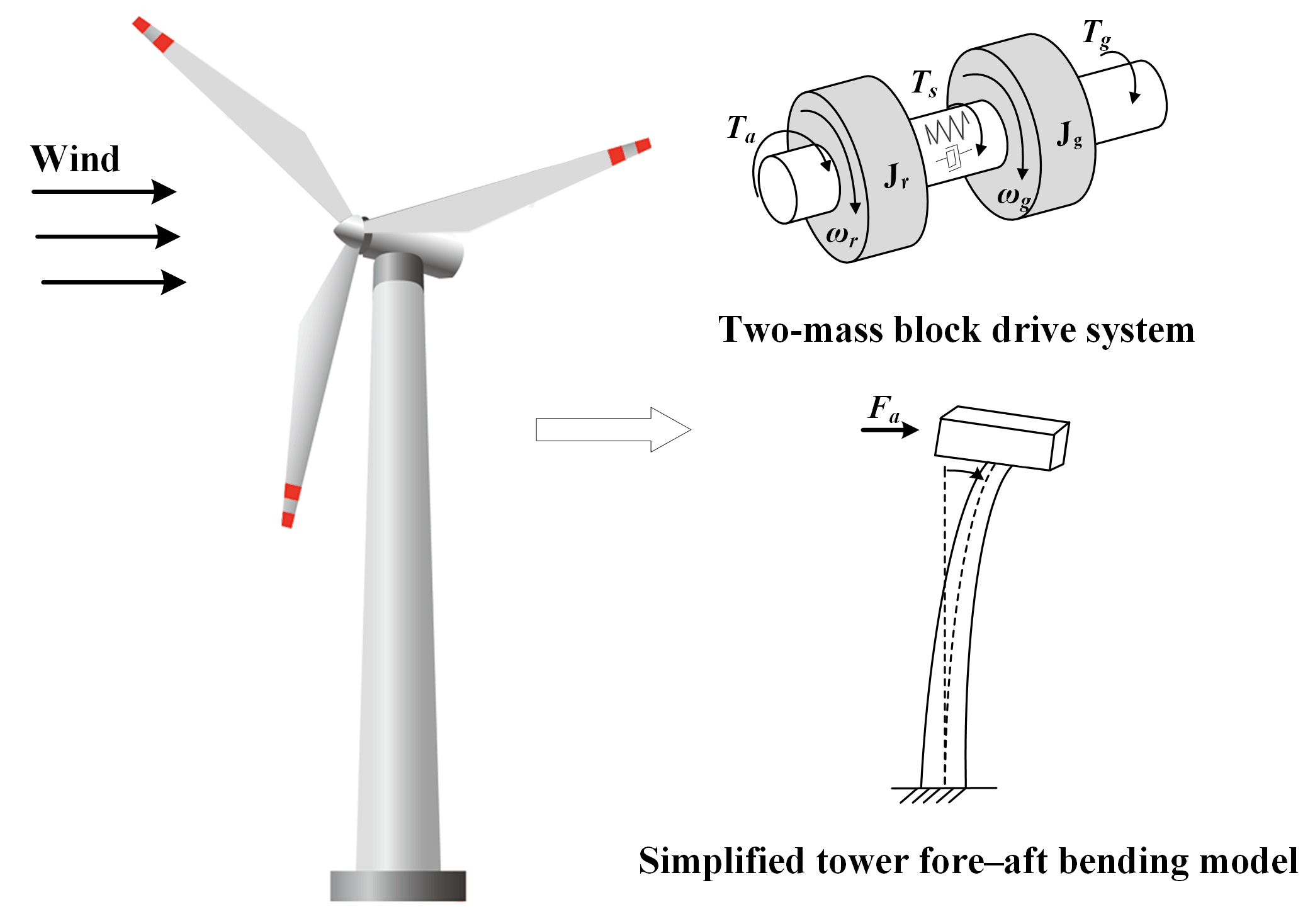
(2) Drivetrain. Depicted in Figure 1, the drivetrain is identified as a two-mass model.

$$\left\{\begin{array}{c}{J}_r{\dot{\omega }}_r=T_a-T_s\hfill \\ J_g{\dot{\omega }}_g=N_{ratio}{T}_s-T_g\hfill \end{array}\right.$$

(3)

The main shaft torque $T_s$ and the torsion angle $\phi$ are calculated as

$$\left\{\begin{array}{c}{T}_s=K_d\phi +B_d\dot{\phi }\hfill \\ \dot{\phi }={\omega }_r-{\omega }_g{N}_{ratio}\hfill \\ {\omega }_g={\displaystyle \frac{{\omega }_r}{N_{ratio}}}\hfill \end{array}\right.$$

(4)

(3) Tower dynamics. Pneumatic thrust $F_a$ causes flexible deformation in the front and rear of the tower, resulting in displacement of the tower top $x_t$. Therefore, the tower is represented as a spring–damping–mass system.

$$F_a=m_{te}{\ddot{x}}_t+B_t{\dot{x}}_t+K_t{x}_t$$

(5)

$m_{te}$, $B_t$, and $K_t$ represent the equivalent modal mass, damping coefficient, and spring coefficient, respectively. The detailed parameters are listed in

Table 1. Parameter specification of the wind turbine model.

Symbol	Parameter	Value
$P_r$	Rated power	5 MW
$v_{in}$	Cut-in wind speed	3 m/s
$V_{rated}$	Rated wind speed	11.4 m/s
$V_{out}$	Cut-out wind speed	25 m/s
$\rho$	Air density	1.2231 kg/m3
R	Rotor radius	63 m
${\omega }_{rated}$	Rated rotor speed	12.1 rpm
$N_{ratio}$	Gear box ratio	0.0103
$J_r$	Rotor inertia	38,677,060 kgm2
$J_g$	Generator inertia	534.116 kgm2
$K_d$	Drivetrain torsional stiffness coefficient	867,637,000 Nm/rad
$B_d$	Drivetrain torsional damping coefficient	6,215,000 Nm/(rad/s)
$m_b$	Single blade mass	17,740 kg
$m_h$	Hub mass	56,780 kg
$m_n$	Nacelle mass	240,000 kg
$m_t$	Tower mass	347,460 kg
$f_n$	Natural frequency of first tower fore–aft bending model	0.32 Hz
$d_s$	Tower structural damping ratio	0.01
${\tau }_{\beta }$	Inertia time constant of pitch actuator	0.2
${\tau }_g$	Inertia time constant of generator	0.02
$\eta$	Generator efficiency	0.944

.

$$\left\{\begin{array}{c}{m}_{te}=3m_b+m_h+m_n+0.25m_t\hfill \\ B_t=4\pi m_{te}{f}_n{d}_s\hfill \\ K_t=m_{te}{\left(2\pi f_n\right)}^2\hfill \end{array}\right.$$

(6)

Consider the first-order fore–aft bending modes, causing relative changes in wind speed acting on the WT.

$$v_r=v-{\dot{x}}_t$$

(7)

For a hub height $H_t$, the equivalent fore–aft bending moment $M_t$ at the tower base satisfies

$$M_t=H_t\left(K_t{x}_t+B_t{\dot{x}}_t\right)$$

(8)

(4) Generator. The generator is treated as a one-order inertia model:

$$\left\{\begin{array}{c}{\dot{T}}_g{\tau }_g-T_g^{ref}+T_g=0\hfill \\ P_g\approx \eta {\omega }_g{T}_g\hfill \end{array}\right.$$

(9)

${\tau }_g$ is the inertia time constant and $T_g^{ref}$ is the generator torque reference value.

(5) Pitch actuator. The pitch control system is described by a one-order inertia model, which is as follows:

$$\dot{\beta }{\tau }_{\beta }-{\beta }^{ref}+\beta =0$$

(10)

${\tau }_{\beta }$ is the inertia time constant of the pitch control system and ${\beta }^{ref}$ is the reference value of the pitch angle.

2.2. Model Linearization

To analyze a nonlinear dynamic system, the small-signal method is utilized. Specifically, a small disturbance is imported at a specific equilibrium point for the state equation. Then the first-order approximation of Taylor expansion is applied for linearization. Then, the incremental model is obtained.

(1)  Aerodynamics.

$$\mathrm{\Delta }{T}_a={\displaystyle \frac{\partial T_a}{\partial {\omega }_r}}\mathrm{\Delta }{\omega }_r+{\displaystyle \frac{\partial T_a}{\partial v_r}}\mathrm{\Delta }{v}_r+{\displaystyle \frac{\partial T_a}{\partial \beta }}\mathrm{\Delta }\beta$$

(11)

(2)  Drivetrain.

$$\left\{\begin{array}{c}\mathrm{\Delta }\dot{{\omega }_r}={\displaystyle \frac{1}{J_b}}(\mathrm{\Delta }{T}_a-K_d\mathrm{\Delta }\phi -B_d\mathrm{\Delta }\dot{\phi })\hfill \\ \mathrm{\Delta }\dot{{\omega }_g}={\displaystyle \frac{N_{ratio}}{J_g}}(K_d\mathrm{\Delta }\phi +B_d\mathrm{\Delta }\dot{\phi }-{\displaystyle \frac{\mathrm{\Delta }{T}_g}{N_{ratio}}})\hfill \\ \mathrm{\Delta }\dot{\phi }=\mathrm{\Delta }{\omega }_r-N_{ratio}\mathrm{\Delta }{\omega }_g\hfill \end{array}\right.$$

(12)

(3)  Tower.

$$\left\{\begin{array}{c}\mathrm{\Delta }{\ddot{x}}_t={\displaystyle \frac{1}{m_{te}}}(\mathrm{\Delta }{F}_a-K_t\mathrm{\Delta }{x}_t-B_t\mathrm{\Delta }{\dot{x}}_t)\hfill \\ \mathrm{\Delta }{F}_a={\displaystyle \frac{\partial F_a}{\partial {\omega }_r}}\mathrm{\Delta }{\omega }_r+{\displaystyle \frac{\partial F_a}{\partial \beta }}\mathrm{\Delta }\beta +{\displaystyle \frac{\partial F_a}{\partial v_r}}\mathrm{\Delta }{v}_r\hfill \\ \mathrm{\Delta }{M}_t=H_t(K_t\mathrm{\Delta }{x}_t+B_t\mathrm{\Delta }{\dot{x}}_t)\hfill \end{array}\right.$$

(13)

(4)  Generator.

$$\left\{\begin{array}{c}\mathrm{\Delta }\dot{T_g}={\displaystyle \frac{1}{{\tau }_g}}(\mathrm{\Delta }{T}_g^{ref}-\mathrm{\Delta }{T}_g)\hfill \\ \mathrm{\Delta }\dot{P_g}={\displaystyle \frac{\partial P_g}{\partial {\omega }_g}}\mathrm{\Delta }{\omega }_g+{\displaystyle \frac{\partial P_g}{\partial T_g}}\mathrm{\Delta }{T}_g\hfill \end{array}\right.$$

(14)

(5)  Pitch controller.

$$\mathrm{\Delta }\dot{\beta }={\displaystyle \frac{1}{{\tau }_{\beta }}}(\mathrm{\Delta }{\beta }^{ref}-\mathrm{\Delta }\beta )$$

(15)

The incremental state-space representation is expressed as

$$\left\{\begin{array}{c}\mathrm{\Delta }\dot{x}=f(\mathrm{\Delta }x,\mathrm{\Delta }u,\mathrm{\Delta }d)\hfill \\ \mathrm{\Delta }y=g(\mathrm{\Delta }x,\mathrm{\Delta }u,\mathrm{\Delta }d)\hfill \end{array}\right.$$

(16)

where x, y, u, and d are the system state vector, system output, system input, and disturbance, respectively. The corresponding incremental representation is expressed as follows.

$$\left\{\begin{array}{c}\begin{array}{c}\mathrm{\Delta }x={\left[\mathrm{\Delta }\phi \mathrm{\Delta }{\omega }_r\mathrm{\Delta }{\omega }_g\mathrm{\Delta }\beta \mathrm{\Delta }{T}_g\mathrm{\Delta }{x}_t\mathrm{\Delta }{\dot{x}}_t\right]}^T\hfill \\ \mathrm{\Delta }y={\left[\mathrm{\Delta }{\omega }_r\mathrm{\Delta }{\omega }_g\mathrm{\Delta }{M}_t\mathrm{\Delta }{T}_s\mathrm{\Delta }{P}_g\right]}^T\hfill \\ \mathrm{\Delta }u={\left[\mathrm{\Delta }\beta \mathrm{\Delta }{T}_g\right]}^T\hfill \\ \mathrm{\Delta }d=\mathrm{\Delta }{v}_r\hfill \end{array}\hfill \end{array}\right.$$

(17)

Given that the main objective of the partial-load region is to achieve maximum wind energy capture, which is equivalent to the maintenance of the maximum power coefficient point, there is no requirement to activate the pitch mechanism for wind energy curtailment. Therefore, the inputs to the partial-load region do not contain $\beta$, and their incremental expression is $\mathrm{\Delta }u=\mathrm{\Delta }{T}_g$.

3. Controller Design

3.1. Model Bank Construction Based on GAP Metric

(1) GAP Metric Theory. As a powerful tool, the gap metric theory is introduced to describe the dynamical difference between the linear system with uncertainty. For a linear system, the corresponding rational transfer matrix is calculated by taking normalized coprime factorization as follows.

$$\left\{\begin{array}{c}H\left(s\right)=E\left(s\right)F^{-1}\left(s\right)\hfill \\ \tilde{F}\left(s\right)F\left(s\right)+\tilde{E}\left(s\right)E\left(s\right)=I\hfill \\ \tilde{F}\left(s\right)=F{(-s)}^T\hfill \\ \tilde{E}\left(s\right)=E{(-s)}^T\hfill \end{array}\right.$$

(18)

where $F\left(s\right)$ and $E\left(s\right)$ represent the numerator and denominator polynomials, respectively. Then the transfer functions of the gap between two linear systems are denoted as $H_1\left(s\right)$ and $H_2\left(s\right)$.

$$\delta (H_1,H_2)=max\{\overline{\delta }(H_1,H_2),\overline{\delta }(H_2,H_1)\}$$

(19)

where $\overline{\delta }\left(H_1,H_2\right)$ is defined as the direct gap:

$$\overline{\delta }\left(H_1,H_2\right)=\underset{\forall \varphi \in H_{\infty }}{min}{∥\left[\begin{array}{c}{F}_1\\ E_1\end{array}\right]-\left[\begin{array}{c}{F}_2\\ E_2\end{array}\right]\varphi ∥}_{\infty }$$

(20)

It is noted that the two models with similar dynamic responses have a close gap, which is near zero. In contrast, the gap between two different systems is close to 1. The two linear systems with a close gap are suitable for one common controller with stabilization.

(2) Model Bank Construction. The model bank is constructed by calculating the gap metrics of the linearized WT model. First, the operational region is divided into N parts equally. Each sub-region corresponds to a specific wind speed point $v_i$. Second, the i-th WT model is linearized at the wind speed point $v_i$. Then, the gap metric between each linearized model is calculated, denoted as $\delta (i,j)$. Finally, a gap metric matrix is obtained as shown in Figure 2. Specifically, the division interval is set to 1 m/s, and the wind speed point in the partial-load region ranges from 3.5 m/s to 10.5 m/s, so N is 8 (Figure 2a). The wind speed point in the full-load region ranges from 11.5 m/s to 24.5 m/s, which gives N as 14 (Figure 2b). Obviously, the closer the two wind speed regions, the smaller the gap metrics of the corresponding model. Further, the selection of the gap metric threshold is vital for model bank construction. Usually, it depends on the system nonlinearity and trial preferences. A smaller threshold increases the number of selected models, improving the approximation accuracy of the linear system. However, this results in an expanded model library and more frequent controller switching. Conversely, a larger threshold reduces the model library size, simplifying preliminary preparation and lowering switching frequency, but at the cost of increased switching magnitude. To overcome it, an optimal soft-switching strategy is proposed to enhance the selection tolerance. Algorithm 1 illustrates the implementation step of the model bank construction. In this paper, $\lfloor C_k\delta (i,j)\rfloor =1$ is chosen as the threshold, and then $M=5$ and $M=12$ are chosen to build the model bank in the partial-load and full-load areas, respectively.

Algorithm 1: Model Bank Construction

Step 1: Initialize i=1, j=1, where i and j represent the rows and columns of the gap metric matrix, respectively. i, j = 1, 2,..., N. Step 2: Filter models based on gap values and determine the number of models in the model bank, M.    if $\lfloor C_k\delta (i,j)\rfloor <1$       j = j + 1   else       i = j       j = i + 1       M = M + 1   end $C_k=10$ is the amplification factor. Step 3: Record M models that exceed the threshold during the algorithm calculation process, and form a model bank.

3.2. Optimization Problem

Based on the model bank, the multiple linear controller is designed. The switch unit selects the proper MPC based on the measured operational point. Owing to the excellent tracking performance with constraints, the linear MPC is employed as the local linear controller. Then, a constrained convex optimization problem is solved by utilizing the Quadratic Programming (QP) algorithm.

$$\begin{array}{cc}\hfill J_m=\sum _{i=0}^{N_c-1}& [{(y_m(k+i)-y_{ref})}^T{Q}_m(y_m(k+i)-y_{ref})+u_m{(k+i)}^T{R}_m{u}_m(k+i)\hfill \\ & + \mathrm{\Delta }{u}_m{(k+i)}^T{S}_m\mathrm{\Delta }{u}_m(k+i)]\hfill \end{array}$$

(21)

$$\begin{array}{c}\hfill y_m(k+i+1)=C_m{x}_m(k+i)\forall i\in 1,\dots ,N_c-1\end{array}$$

(22)

subject to:

$$\left\{\begin{array}{c}{y}_{min}\le y\le y_{max}\hfill \\ u_{min}\le u\le u_{max}\hfill \\ \mathrm{\Delta }{u}_{min}\le \mathrm{\Delta }u\le \mathrm{\Delta }{u}_{max}\hfill \end{array}\right.$$

(23)

$J_m$ represents the cost function of the m-th MPC. $x_m$ and $u_m$ represent the state variables and input variables in the m-th linear model. $Q_m$, $S_m$ and $R_m$ represent the tuning weight matrices, respectively. These weight matrices are used to adjust the objective by penalizing the corresponding quadratic terms. Moreover, the constraints also consider the changing rate limitation of the control input. This prevents the transient failure risks of the actuator such as the pitch and generator controller.

3.3. Soft-Switching Multiple MPC

To achieve the dynamic performance, multiple MPC is designed based on the model bank. Each local MPC controller is designed according to the instantaneous wind speed. However, the controller switching would result in instability. To overcome this, a hybrid membership function is proposed to suppress the sudden control change and smooth the controller output. In Figure 3a, it is seen that a set of triangular functions is constructed based on the steady-state points from MPC2 to MPC4. Meanwhile, a set of trapezoidal functions is established based on the steady-state points for MPC1 and MPC5, and together, they form a hybrid membership function for the partial-load region. Similarly, the membership function of the full-load region is also constructed, as shown in Figure 3b. To ensure local MPC control accuracy at its designated wind speed, positioning the support points and peak point of the triangular membership function at adjacent model wind speeds and the current model wind speed, respectively, is optimal. This applies equally to the trapezoidal membership function. Trapezoidal functions are placed at operating region boundaries (partial- and full-load regions) because while entering or exiting these regions, model switching is unnecessary, and the function output must remain at unity. Then, a smooth transition of weights from 1 to 0 and back to 1 is achieved between adjacent functions. These seven membership functions facilitate a soft-switching strategy for the MMPC, which is defined as soft switch multiple MPC. Figure 4 presents the structure of SSMMPC. The detailed implementation is shown in Algorithm 2.

Algorithm 2: Soft Switching Strategy

Step 1: Design MPC controllers for each linear model. Step 2: Design membership functions for trapezoidal $W_i^{tra}\left(v_r\right)$ and triangular $W_i^{tri}\left(v_r\right)$ based on the output response of a single MPC controller in different step wind speed ranges. Step 3: Using the input wind speed $v_r$ as the membership function variable, establish a global weight allocation function to assign weights to the control signals of each controller.                            $W_i\left(v_r\right)=\left\{\begin{array}{c}{W}_i^{tra}\left(v_r\right)i=1,M\hfill \\ W_i^{tri}\left(v_r\right)1<i<M\hfill \end{array}\right.$ Step 4: Take the weighted sum of the output signals $u_i$ from a single controller as the global control action $u_{all}$, and smooth the control signal oscillation.                                        $u_{all}={\displaystyle \sum _{i=1}^M}{W}_i{u}_i$

3.4. Stability Proof of SSMMPC

Lyapunov’s second method is utilized to analyze the stability of MPC and SSMMPC sequentially. The system is asymptotically stable if the condition $V(k+1)-V\left(k\right)<0$ is satisfied.

(1) MPC. The Lyapunov function is defined as $V\left(k\right)=J\left(k\right)$. For simplicity, assume that each MPC have the same prediction and control horizons, then

$$\begin{array}{cc}\hfill V_m\left(k\right)=\sum _{i=0}^{N_c-1}& \left({∥y_m(k+i)-y^{ref}∥}_{Q_m}^2+{∥u_m(k+i)∥}_{R_m}^2+{∥\mathrm{\Delta }{u}_m(k+i)∥}_{S_m}^2\right)\hfill \end{array}$$

(24)

$$\begin{array}{cc}\hfill V_m(k+1)=\sum _{i=0}^{N_c-1}& \left({∥y_m(k+i+1)-y^{ref}∥}_{Q_m}^2+{∥u_m(k+i+1)∥}_{R_m}^2+{∥\mathrm{\Delta }{u}_m(k+i+1)∥}_{S_m}^2\right)\hfill \end{array}$$

(25)

Thus, MPC is stable when the following condition is satisfied:

$$\begin{array}{cc}\hfill & {∥y_m(k+N_c)∥}_{Q_m}^2+{∥u_m(k+N_c)∥}_{R_m}^2+{∥\mathrm{\Delta }{u}_m(k+N_c)∥}_{S_m}^2\hfill \\ & <{∥y_m\left(k\right)∥}_{Q_m}^2+{∥u_m\left(k\right)∥}_{R_m}^2+{∥\mathrm{\Delta }{u}_m\left(k\right)∥}_{S_m}^2\hfill \end{array}$$

(26)

$S_m$ is chosen in the Riccati solution of the LQR problem to guarantee the validity of the aforementioned equation.

(2) SSMMPC. Mathematically, the soft switching between MPC controllers is equal to the switching between different membership functions. Several assumptions are made as follows:

i

   The wind is generated randomly.

ii

$p_i=p_j$.

iii

$p_i={\alpha }_i$.

iv

$\bigcup _{i=1}^M{\alpha }_i=1$.

Here, $p_i$ is the probability that the i-th membership function is activated and ${\alpha }_i$ is the probability of switching to the i-th cost function, $\forall i,j\in (1,2,\dots ,M)$. Therefore, SSMMPC is stable if

$$\begin{array}{cc}\hfill \sum _{m=1}^M& {\alpha }_m\left({∥y_m(k+N_c)∥}_{Q_m}^2+{∥u_m(k+N_c)∥}_{R_m}^2+{∥\mathrm{\Delta }{u}_m(k+N_c)∥}_{S_m}^2\right)\hfill \\ & <\sum _{m=1}^M{\alpha }_m\left({∥y_m\left(k\right)∥}_{Q_m}^2+{∥u_m\left(k\right)∥}_{R_m}^2+{∥\mathrm{\Delta }{u}_m\left(k\right)∥}_{S_m}^2\right)\hfill \end{array}$$

(27)

Since ${\alpha }_i\ge 0$, which can be re-expressed as

$$\begin{array}{cc}\hfill \sum _{m=1}^M& \left({∥y_m(k+N_c)∥}_{Q_m}^2+{∥u_m(k+N_c)∥}_{R_m}^2+{∥\mathrm{\Delta }{u}_m(k+N_c)∥}_{S_m}^2\right)\hfill \\ & <\sum _{m=1}^M\left({∥y_m\left(k\right)∥}_{Q_m}^2+{∥u_m\left(k\right)∥}_{R_m}^2+{∥\mathrm{\Delta }{u}_m\left(k\right)∥}_{S_m}^2\right)\hfill \end{array}$$

(28)

Clearly, the stability of SSMMPC can also be guaranteed when inequality (26) is established.

4. Case Studies

4.1. Experimental Design

We design several experiments to answer the following questions:

Q1: Can our designed soft switch rule keep the controller stable without causing large ripples?

Q2: Can our proposed SSMMPC adapt multiple linear models in a wide range of operational points?

Q3: Can our proposed SSMMPC controller exhibit excellent performance in terms of maximum power point tracking, torque oscillation suppression, and tower bending moment reduction?

To answer these, simulation-based validation was conducted across both the partial-load and full-load operational regions. Firstly, the effectiveness of the soft switching strategy is evaluated under turbulent wind conditions in the partial-load region. The MPC [17] and MMPC [22] are imported for comparison. After that, the performance in the full-load region of these MPC-based controllers is discussed in two typical scenarios: turbulent wind and extreme gust conditions. Three aspects are involved, including power reference tracking, control signal oscillation suppression, and fatigue load reduction. All simulations are tested based on the National Renewable Energy Laboratory (NREL) 5MW nonlinear model built on the Matlab/Simulink platform [23] (as shown in Table 1) and the same controller parameters (weight matrices $Q_m$, $R_m$ and $S_m$) are employed for validation. The controller sampling time is set to 0.0125 s, with a prediction horizon of 10 and a control horizon of 2. Turbulent wind is generated using TurbSim. A turbulence intensity of 0.15 is used for the partial-load region, and 0.10 is used for the full-load region. The Kaimal turbulence model is employed. Notably, the variables $T_s$ and $M_t$ in the system output vector are unmeasurable. $W_g$, $P_g$, $\phi$, and $x_t$ are assumed to be measurable in this study, and the remaining variables are estimated using Kalman observers. However, since this aspect is not the focus of the research, no further discussion is provided.

4.2. Case 1: Turbulent Wind in Partial-Load Region

(1) Maximum Power Point Tracking. Figure 5 shows the simulation results of the wind profiles generated by TurbSim with a turbulence intensity of 0.15 for both winds, and the maximum power point tracking of the wind turbine at a mean wind speed of 8 m/s. The MPC in this case is designed based on the 5.5 m/s steady-state point; hence, the $C_p$ value of the MPC in Figure 5b is much less effective than the MMPC and SSMMPC in tracking the maximum power coefficient point under 8 m/s turbulent wind.

Table 2. RMSEs of $C_p$ under turbulent wind conditions.

Wind Speed	MPC	MMPC		SSMMPC
(m/s)	RMSE	RMSE	Percentage	RMSE	Percentage
5	0.0188	0.0143	23.82%	0.0140	25.57%
8	0.0654	0.0142	78.32%	0.0142	78.32%

and

Table 3. MAEs of $C_p$ under turbulent wind conditions.

Wind Speed	MPC	MMPC		SSMMPC
(m/s)	MAE	MAE	Percentage	MAE	Percentage
5	0.0112	0.0079	29.35%	0.0075	33.06%
8	0.0547	0.0084	84.72%	0.0083	84.85%

show the root mean square errors (RMSE) and mean absolute errors (MAE) of the $C_p$ tracking for different wind speeds, respectively. The percentage shown means the degree of reduction compared to MPC. From 5 m/s to 8 m/s, the larger the average wind speed, the larger the standard deviation of the wind profile, which leads to a larger wind speed span and a larger range of turbine operating points, reinforcing the advantage that the MMPC can be freely switched at various operating points. Obviously, the RMSE of MMPC and SSMMPC relative to MPC is significantly reduced by 78.32% simultaneously when the input wind speed becomes 8 m/s, while the MAE is reduced by about 84% at the same time. This sufficiently indicates that the proposed SSMMPC inherits the advantages of MMPC and provides stable tracking of the maximum power point.

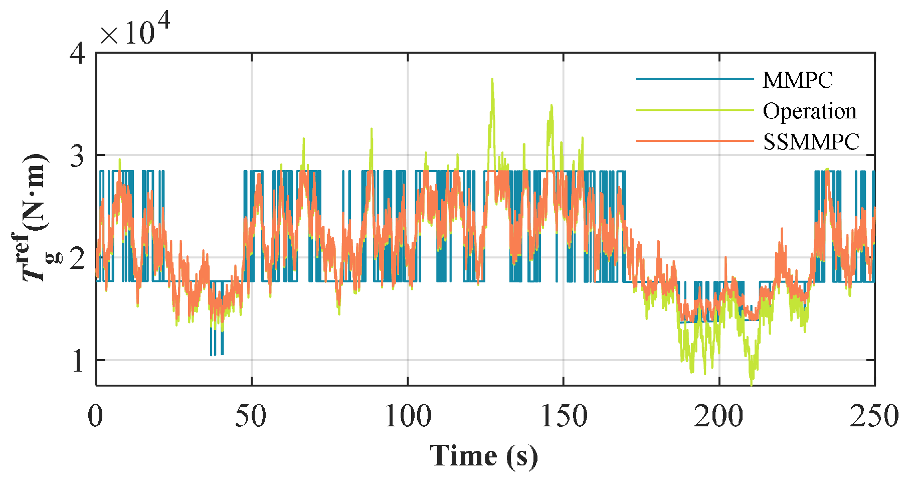
(2) Control Signal Oscillation Suppression. Figure 6 illustrates the variation of control signals for SSMMPC and MMPC under 8 m/s turbulent wind. Since the steady-state point of ${T_g}^{ref}$ is not fixed in the partial-load region, the slave MPC can only guarantee the tracking state at its own designed operating point, which results in the control signals oscillating frequently among the three MPC signals when the MMPC is switched. SSMMPC relies on the membership function to achieve stable tracking of the operating point and smooth switching of the controller signals, which is particularly evident between 50 s and 170 s in Figure 6. Overall, the control signal ${T_g}^{ref}$ of the SSMMPC is more stable than that of the MMPC, allowing better tracking of the operating point.

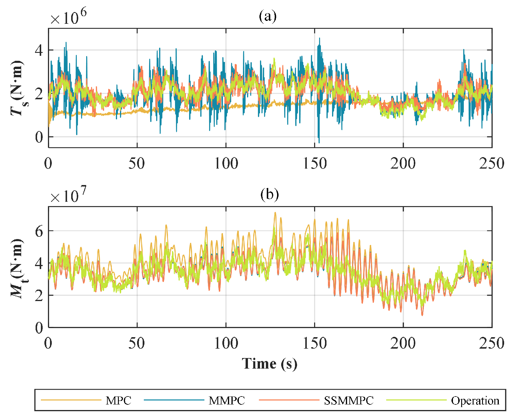
(3) Fatigue Load Reduction. Figure 7 exhibits the fluctuations of $T_s$ and $M_t$ under turbulent winds with a mean speed of 8 m/s. MPC has a small fluctuation amplitude but does not track the operating point at all. Both $T_s$ and $M_t$ of SSMMPC and MMPC track the stable operating point, but the $T_s$ of MMPC oscillates much more than that of SSMMPC due to the ${T_g}^{ref}$ jitter. From the damage equivalent load (DEL) values in

Table 4. DELs of the three strategies under turbulent wind conditions.

Wind Speed	MPC		MMPC		SSMMPC
(m/s)	${\mathbf{T}}_{\mathbf{s}}$ (MNm)	${\mathbf{M}}_{\mathbf{t}}$ (MNm)	${\mathbf{T}}_{\mathbf{s}}$ (MNm)	${\mathbf{M}}_{\mathbf{t}}$ (MNm)	${\mathbf{T}}_{\mathbf{s}}$ (MNm)	${\mathbf{M}}_{\mathbf{t}}$ (MNm)
5	0.316	22.279	2.254	22.650	1.396	22.494
8	1.229	76.996	6.428	63.296	3.043	62.845

, it can be seen that the DEL of $T_s$ for the proposed method is significantly improved with respect to MMPC by 52.67%. The absence of pitch control in partial-load regions resulted in weak $M_t$ changes in MMPC and SSMMPC. Instead, the MPC makes the DEL of $M_t$ larger due to the loss of operating point tracking capability, which is roughly an 18% increase compared to the two advanced controllers.

In summary, the well-performed SSMMPC is verified in the partial-load region in terms of control signal oscillation suppression, operating point tracking, fatigue load reduction and maximum power tracking, especially in $T_s$ fatigue load reduction and ${T_g}^{ref}$ oscillation suppression.

4.3. Case 2: Turbulent Wind in Full-Load Region

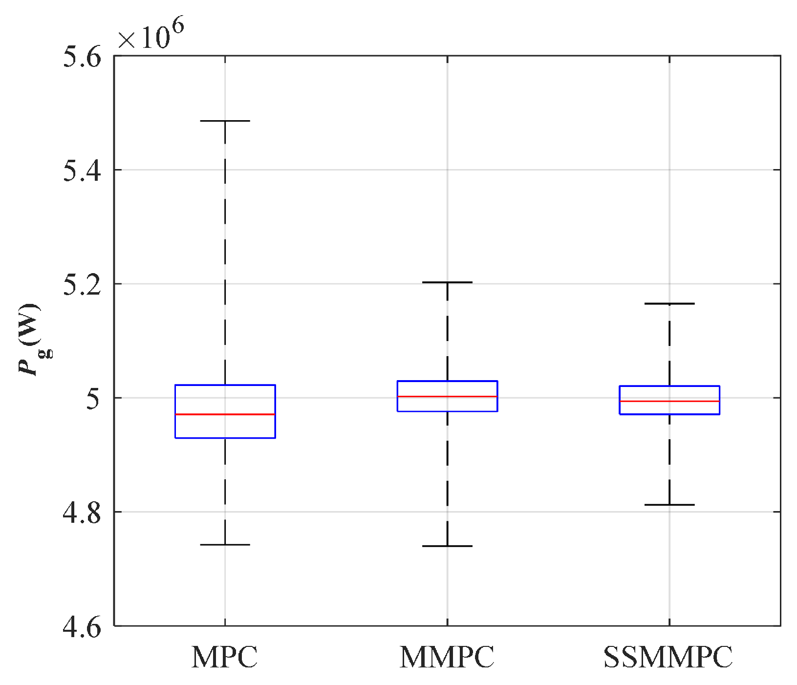
(1) Power Reference Tracking. In this case, simulations were performed under turbulent winds with mean values of 14 m/s, 18 m/s, and 22 m/s (Figure 8a), and the results for 18 m/s are plotted. To visualize the data distribution, Figure 9 presents the box and whisker plot of the output power. It is found that the median of MPC is furthest away from the 5 MW reference value due to the limited ability to track at non-designed operating points. The box height of the SSMMPC is close to that of the MMPC; however, the end lines are shorter. This indicates that the $P_g$ data is more centralized and the reference power tracking is more effective. The advantages of the proposed method in power tracking are confirmed again.

Table 5. RMSEs of active power under turbulent wind conditions.

Wind Speed	MPC	MMPC		SSMMPC
(m/s)	RMSE (MW)	RMSE (MW)	Percentage	RMSE (MW)	Percentage
14	0.070	0.043	38.90%	0.041	41.88%
18	0.112	0.054	51.66%	0.045	60.20%
22	0.177	0.110	37.97%	0.081	54.16%

presents the RMSEs at different wind speeds. Interestingly, as the average wind speed increases, the RMSE of SSMMPC increases from 4.87% to 26.11% compared to MMPC, which is a more significant optimization result. The increase in MAE (

Table 6. MAEs of active power under turbulent wind conditions.

Wind Speed	MPC	MMPC		SSMMPC
(m/s)	MAE (MW)	MAE (MW)	Percentage	MAE (MW)	Percentage
14	0.0519	0.0314	39.40%	0.0305	41.24%
18	0.0709	0.0404	42.98%	0.0343	51.72%
22	0.0972	0.0840	13.61%	0.0640	34.18%

) is not as significant as RMSE, and the optimized value increases from 3.04% to 23.81% with wind speed, showing a gradual increase trend with wind speed.

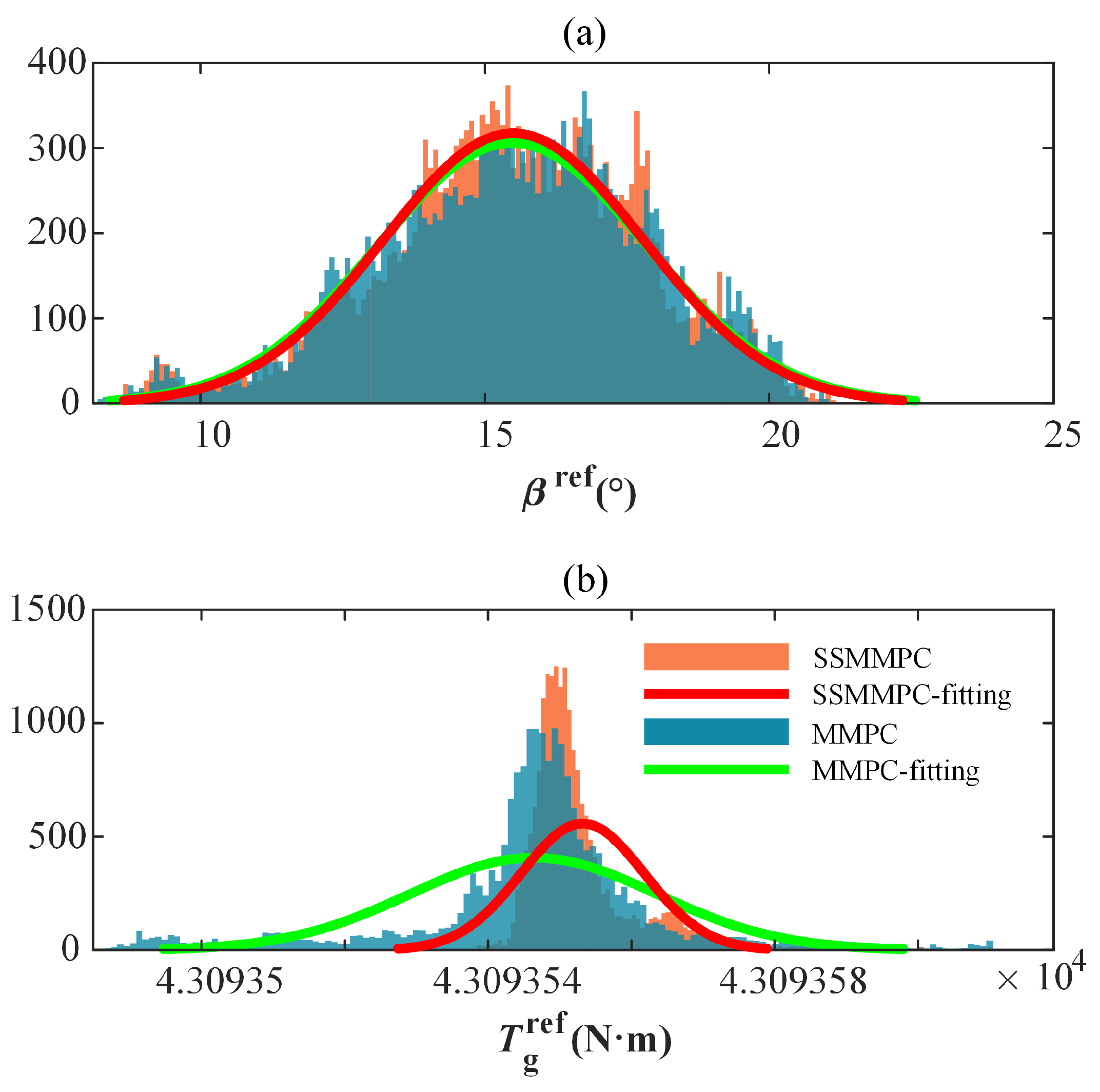
(2) Control Signal Oscillation Suppression. Figure 10 and Figure 11 illustrate the variations of the control signals ${\beta }^{ref}$ and ${T_g}^{ref}$ for MMPC and SSMMPC, as well as the histograms with normal fitting. Overall, the generator torque and pitch angle of SSMMPC are more stable and fluctuate less than those of MMPC. Further, owing to the stochastic nature of wind speed excitation, ${\beta }^{ref}$ and ${T_g}^{ref}$ approximately reveal a normal distribution, which validates the reliability of the results.

Table 7. Statistical data of control signals under turbulent wind conditions.

Control Signal	Type	MMPC	SSMMPC	Percentage
${\beta }^{ref}$	$\mu$	15.4849	15.5014	\
	$\sigma$	2.3613	2.2821	3.36%
$T_g^{ref}$	$\mu$	43,093.5463	43,093.5532	\
	$\sigma$	0.0172	0.0086	50.15%

presents the statistical results of the fitting normal distribution. It is found that the distribution means of MMPC and SSMMPC are similar. However, the standard deviations of ${\beta }^{ref}$ and ${T_g}^{ref}$ for SSMMPC are decreased by 3.36% and 50.15% compared to MMPC, respectively. The comparison results prove that the generator torque fluctuations are effectively suppressed. The reason is that the proposed SSMMPC utilizes the hybrid membership function to eliminate excessive switching. Thus, it is beneficial to reduce the mechanical stress and possible risk of damage.

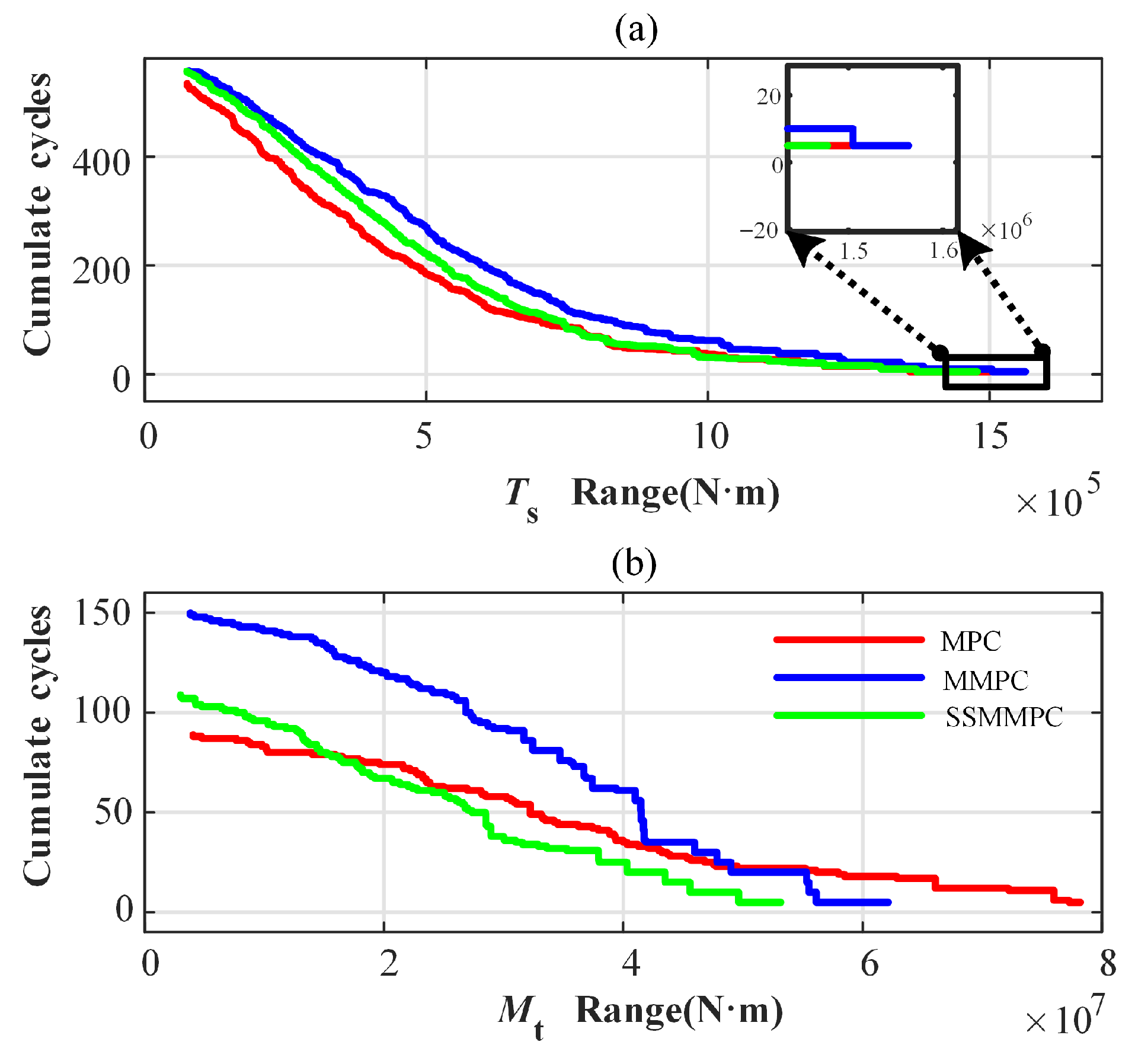
(3) Fatigue Load Reduction. Figure 12 presents a comparison of the main shaft torque and tower bending moment with three different strategies. It is found that the hard-switching MMPC leads to a more pronounced fluctuation compared to SSMMPC due to control signal ripple.

Table 8. DELs of the three strategies under turbulent wind conditions.

Wind Speed	MPC		MMPC		SSMMPC
(m/s)	${\mathbf{T}}_{\mathbf{s}}$ (MNm)	${\mathbf{M}}_{\mathbf{t}}$ (MNm)	${\mathbf{T}}_{\mathbf{s}}$ (MNm)	${\mathbf{M}}_{\mathbf{t}}$ (MNm)	${\mathbf{T}}_{\mathbf{s}}$ (MNm)	${\mathbf{M}}_{\mathbf{t}}$ (MNm)
14	0.922	78.966	1.067	79.848	0.907	63.124
18	1.928	101.943	2.075	81.213	1.915	68.346
22	2.502	142.633	2.522	107.791	2.445	96.585

shows the DELs of $T_s$ and $M_t$. SSMMPC exhibits the strongest robustness in fatigue load reduction under different turbulent wind speeds. Specifically, when the turbulent wind speed is 18 m/s, the DELs of $M_t$ for MMPC and SSMMPC are decreased by 20.33% and 32.96% compared with MPC. Comparably, MMPC’s $T_s$ has a higher DEL than MPC, negatively attributed to MMPC switching oscillations. Excitingly, SSMMPC successfully limits the effect of MMPC’s oscillation on $T_s$, which is optimized by 15.84% at 14 m/s, but the DEL is almost equal to that of MPC. Besides that, the cumulative rainflow cycle in Figure 13 confirms that SSMMPC is beneficial for reducing cycles for both $T_s$ and $M_t$, suggesting that the fatigue loads on the wind turbines are suppressed.

The advantage is that SSMMPC approximates the nonlinear dynamic model of WTs by defining multiple linear models around various operating points, and uses gap metrics as a mathematical tool to construct a set of multiple linear models. By utilizing the hybrid membership function, it ensures soft switching with robust performance. In other words, it is verified that SSMMPC achieves improvements in capturing more energy, better power tracking, lower main shaft torque oscillation, less tower bending and smoother power output.

4.4. Case 3: Extreme Gust in Full-Load Region

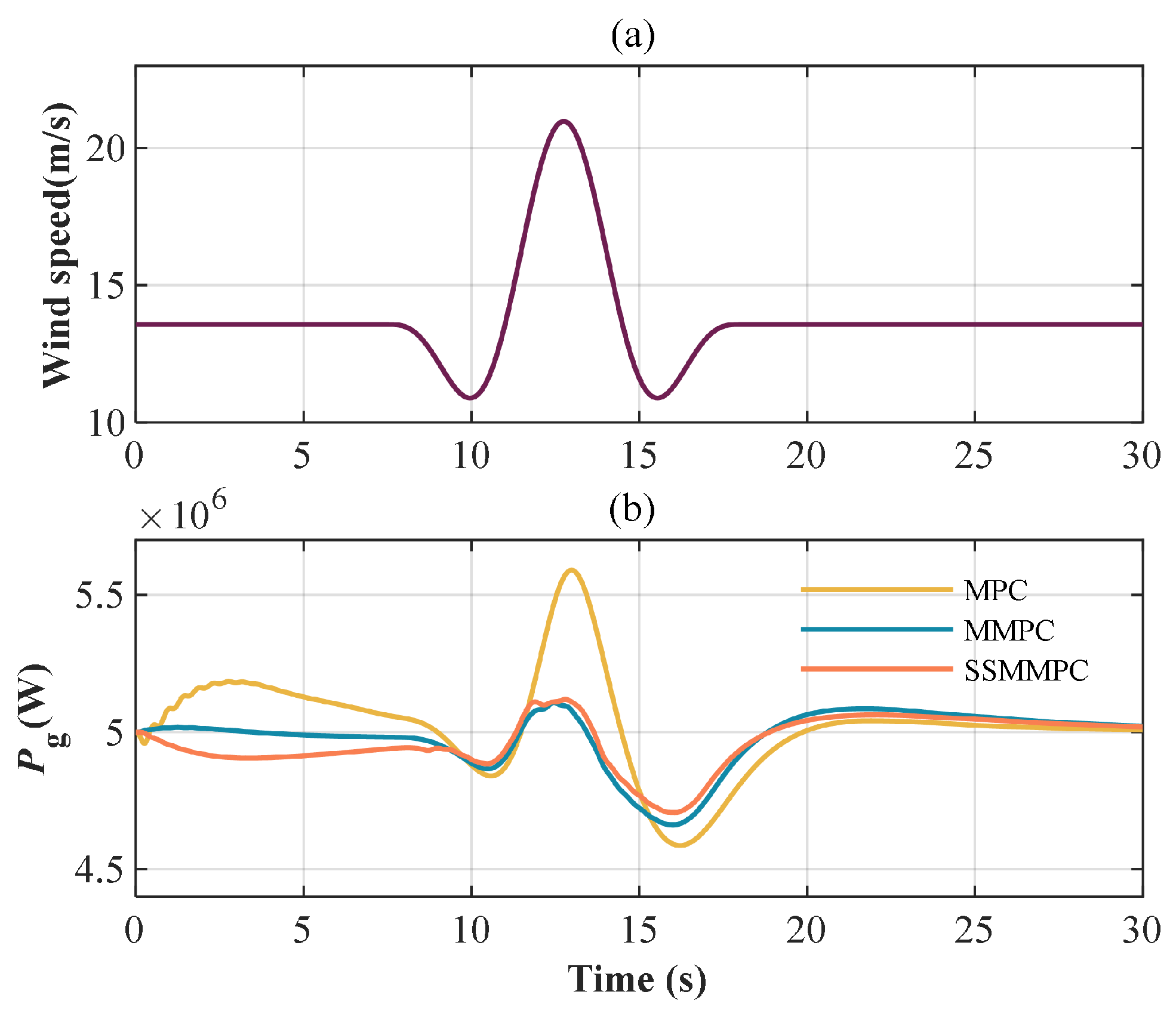
Distinct from turbulent winds, extreme operating gusts vary dramatically over short periods of time. To verify the adaptability of SSMMPC, the time-domain responses of different control strategies are compared under extreme gust conditions. According to the IEC61400 standard [24], an extreme operating gust time series $V\left(t\right)$ is created with an incoming wind speed $V_h$ of 13.5 m/s and a gust amplitude $V_a$ of 10 m/s at the hub height, as shown in Figure 14a, where $T_p$ = 10.5 s is the gust period.

$$\begin{array}{c}V\left(t\right)=\left\{\begin{array}{c}{V}_h-0.37V_a\sin \left({\displaystyle \frac{3\pi (t-10)}{T_p}}\right)(1-\cos \left({\displaystyle \frac{2\pi (t-10)}{T_p}}\right))0\le t\le T_p\hfill \\ V_{h}others\hfill \end{array}\right.\hfill \end{array}$$

(29)

(1) Power Reference Tracking. Different from the turbulent wind, the extreme gusts would lead to rapid fluctuations in wind velocity and power output, as presented in Figure 14b. The power output of MPC reveals the largest fluctuation while the output of MMPC and SSMMPC is smoother. The RMSEs for MPC, MMPC and the SSMMPC are 0.182, 0.108 and 0.100 (MW), respectively. Wide variations in wind speeds over short periods of time can accentuate the advantages of the MMPC. Furthermore, SSMMPC membership function execution time is shortened consequently, leading to a weakening of the oscillation smoothing effect, which is consistent with the phenomenon in other cases.

(2) Control Signal Oscillation Suppression. Figure 15 presents the control signals ${\beta }^{ref}$ and ${T_g}^{ref}$ for MMPC and SSMMPC. Compared to MMPC, the proposed method avoids excessive spikes between 10s and 15s by weighting the outputs of different MPCs and keeps tracking even after the gust stabilizes. Obviously, it is revealed that the generator torque and pitch angle of SSMMPC are smoother and fluctuate less than those of MMPC.

(3) Fatigue Load Reduction. Figure 16 presents the main shaft torque $T_s$ and tower bending moment $M_t$ with MPC, MMPC and SSMMPC under the extreme gust conditions. Owing to the multiple model bank construction, both SSMMPC and MMPC decrease the amplitude of fluctuation compared to MPC in terms of the global trend. For dynamic instantaneous fluctuation, the soft-switching algorithm diminishes the generator’s torque oscillations, consequently mitigating the torque variations impacting the transmission system.

Table 9. DELs of three strategies under extreme gust conditions.

Load	MPC	MMPC		SSMMPC
	DEL (MNm)	DEL (MNm)	Percentage	DEL (MNm)	Percentage
$T_s$	2.034	1.211	40.46%	1.050	48.35%
$M_t$	224.081	146.414	34.66%	133.415	40.46%

calculates the DELs for $T_s$ and $M_t$. The $T_s$ and $M_t$ of SSMMPC are reduced by 48.35% and 40.46%, respectively, compared to MPC. Meanwhile, $T_s$ and $M_t$ are reduced by 13.26% and 8.8%, compared with MMPC. The results confirm that the soft-switching method proposed in this paper is effective in fatigue load suppression.

5. Limitations

The proposed method has three primary limitations:

• The observer significantly impacts overall control performance. This study employs a dynamic Kalman observer that updates its gain at each control interval. This observer is tightly integrated with the proposed MPC strategy. While we cannot guarantee the measurability of outputs $T_s$ and $M_t$, all state variables must be measurable. Otherwise, observer gain computation will fail, causing system shutdown. Additionally, incorporating wind speed disturbances at the input into the measurable sequence is recommended to enhance controller performance.
• The real-time computational load increases due to the potential simultaneous operation of two MPC controllers solving QP problems during membership function transitions, whereas conventional MPC or MMPC frameworks activate only one controller at a time. Nevertheless, emerging cloud–edge collaborative computing architectures and enhanced storage technologies are anticipated to address this computational limitation in future implementations.
• Due to laboratory constraints, physical experiments could not be conducted. The next step involves establishing a hardware-in-the-loop platform to validate the method on physical systems, with this work serving as the foundation for future research.

6. Conclusions

This paper proposed a novel optimal SSMMPC strategy for WTs by considering power tracking and fatigue load reduction simultaneously. Several experiments are conducted for validation. The main conclusions are summarized as follows.

• The traditional linear MPC controllers cannot satisfy optimality for WTs due to the nonlinear steady-state operating point. Meanwhile, the MMPC causes control signal oscillation with excessive switching, especially under varying operating conditions. Current SSMMPC approaches primarily achieve soft switching by ensuring sufficiently small gaps between models, where only one local MPC controller is active at any given time. However, such methods cannot fully eliminate signal discontinuities caused by switching between controllers. Each reduction in the gap size exponentially increases the model library scale. When improperly large gaps are selected, the SSMMPC essentially reduces to conventional MMPC. These would fade the dynamic performance of WTs in the aspects of power reference tracking and fatigue load reduction.
• The import of the gap metric is essential for the model bank size optimization. An improper gap threshold selection would result in severe control signal oscillation or an excessively large model bank size. By utilizing the hybrid membership functions, 1–2 MPC controllers may operate concurrently at any instant, enabling genuine soft transitions that mitigate excessive fluctuations in control signals under turbulent winds and extreme gusts. Besides that, the stability of SSMMPC is proven by utilizing Lyapunov’s second method.
• The proposed SSMMPC exhibits excellent performance in fatigue load suppression, power reference tracking, and control signal smoothing under turbulent wind conditions in both the partial-load region and full-load region. Compared with MPC, the DEL of the tower bending moment $M_t$ is reduced by 32.96% and the RMSE of power $P_g$ is reduced by 60.20% under the 18m/s turbulent wind condition. In addition, the standard deviation of the control signal ${T_g}^{ref}$ is reduced by 50.15% against MMPC.

References

1. Hu, Z.; Su, R.; Ling, K.V.; Guo, Y.; Ma, R. Resilient Event-Triggered MPC for Load Frequency Regulation With Wind Turbines Under False Data Injection Attacks. IEEE Trans. Autom. Sci. Eng. 2023, 21, 7073–7083. [Google Scholar] [CrossRef]
2. Liu, X.; Feng, L.; Kong, X.; Guo, S.; Lee, K.Y. Tube-Based Stochastic Model Predictive Control With Application to Wind Energy Conversion System. IEEE Trans. Control Syst. Technol. 2023, 31, 2173–2187. [Google Scholar] [CrossRef]
3. Hu, Y.; Chau, T.K.; Zhang, X.; Iu, H.H.C.; Fernando, T.; Fan, D. A Novel Adaptive Model Predictive Control Strategy for DFIG Wind Turbine With Parameter Variations in Complex Power Systems. IEEE Trans. Power Syst. 2023, 38, 4582–4592. [Google Scholar] [CrossRef]
4. Yao, Q.; Ma, B.; Zhao, T.; Hu, Y.; Fang, F. Optimized Active Power Dispatching of Wind Farms Considering Data-Driven Fatigue Load Suppression. IEEE Trans. Sustain. Energy 2023, 14, 371–380. [Google Scholar] [CrossRef]
5. Yang, J.; Zheng, S.; Song, D.; Su, M.; Yang, X.; Joo, Y.H. Comprehensive Optimization for Fatigue Loads of Wind Turbines in Complex-Terrain Wind Farms. IEEE Trans. Sustain. Energy 2021, 12, 909–919. [Google Scholar] [CrossRef]
6. Wang, T.; Jin, M.; Li, Y.; Wang, J.; Wang, Z.; Huang, S. Adaptive Damping Control Scheme for Wind Grid-Connected Power Systems With Virtual Inertia Control. IEEE Trans. Power Syst. 2022, 37, 3902–3912. [Google Scholar] [CrossRef]
7. Liu, B.; Zhao, J.; Huang, Q.; Milano, F.; Zhang, Y.; Hu, W. Nonlinear Virtual Inertia Control of WTGs for Enhancing Primary Frequency Response and Suppressing Drivetrain Torsional Oscillations. IEEE Trans. Power Syst. 2021, 36, 4102–4113. [Google Scholar] [CrossRef]
8. Hawari, Q.; Kim, T.; Ward, C.; Fleming, J. A robust gain scheduling method for a PI collective pitch controller of multi-MW onshore wind turbines. Renew. Energy 2022, 192, 443–455. [Google Scholar] [CrossRef]
9. Tang, S.; Tian, D.; Wu, X.; Huang, M.; Deng, Y. Wind turbine load reduction based on 2DoF robust individual pitch control. Renew. Energy 2022, 183, 28–40. [Google Scholar] [CrossRef]
10. Luo, H.; Hu, Z.; Zhang, H.; Chen, H. Coordinated Active Power Control Strategy for Deloaded Wind Turbines to Improve Regulation Performance in AGC. IEEE Trans. Power Syst. 2019, 34, 98–108. [Google Scholar] [CrossRef]
11. Tang, X.; Yin, M.; Shen, C.; Xu, Y.; Dong, Z.Y.; Zou, Y. Active Power Control of Wind Turbine Generators via Coordinated Rotor Speed and Pitch Angle Regulation. IEEE Trans. Sustain. Energy 2019, 10, 822–832. [Google Scholar] [CrossRef]
12. Xu, Y.; Jia, L.; Peng, D.; Yang, W. Iterative Neuro-Fuzzy Hammerstein Model Based Model Predictive Control for Wind Turbines. IEEE Trans. Ind. Appl. 2023, 59, 6501–6512. [Google Scholar] [CrossRef]
13. Kazda, J.; Cutululis, N.A. Model-Optimized Dispatch for Closed-Loop Power Control of Waked Wind Farms. IEEE Trans. Control Syst. Technol. 2020, 28, 2029–2036. [Google Scholar] [CrossRef]
14. Sinner, M.M.; Petrovic, V.; Langidis, A.; Neuhaus, L.; Hoelling, M.; Kuehn, M.; Pao, L.Y. Experimental Testing of a Preview-Enabled Model Predictive Controller for Blade Pitch Control of Wind Turbines. IEEE Trans. Control Syst. Technol. 2022, 30, 583–597. [Google Scholar] [CrossRef]
15. Wald, D.; Johnson, K.; Bay, C.J.; King, J.; Chintala, R. Grid-Interactive Electric Vehicle and Building Coordination Using Coupled Distributed Control. In Proceedings of the 2022 American Control Conference (ACC), Atlanta, GA, USA, 8–10 June 2022; pp. 2539–2545. [Google Scholar]
16. Bai, G.; Huang, S.; Feng, Y.; Wu, Q.; Tan, L.; Guo, T. MPC-Based Droop Control Scheme for Fatigue Load Suppression in Wind Farms Based on Asynchronous Distributed Manner. IEEE Trans. Ind. Inform. 2024, 20, 12305–12316. [Google Scholar] [CrossRef]
17. Yao, Q.; Hu, Y.; Deng, H.; Luo, Z.; Liu, J. Two-degree-of-freedom active power control of megawatt wind turbine considering fatigue load optimization. Renew. Energy 2020, 162, 2096–2112. [Google Scholar] [CrossRef]
18. Li, T.; Yang, J.; Ioannou, A. Data-driven control of wind turbine under online power strategy via deep learning and reinforcement learning. Renew. Energy 2024, 234, 121265. [Google Scholar] [CrossRef]
19. Wang, H.; Yang, Z.; Chen, Z.; Liang, J.; Li, G.; Yang, J.; Hu, S. Multiple Adaptive Model Predictive Controllers for Frequency Regulation in Wind Farms. IEEE Trans. Energy Convers. 2023, 38, 15–26. [Google Scholar] [CrossRef]
20. Gavgani, B.M.; Farnam, A.; De Kooning, J.D.M.; Crevecoeur, G. Efficiency Enhancements of Wind Energy Conversion Systems Using Soft Switching Multiple Model Predictive Control. IEEE Trans. Energy Convers. 2022, 37, 1187–1199. [Google Scholar] [CrossRef]
21. Ebadollahi, S.; Saki, S. Wind Turbine Torque Oscillation Reduction Using Soft Switching Multiple Model Predictive Control Based on the Gap Metric and Kalman Filter Estimator. IEEE Trans. Ind. Electron. 2018, 65, 3890–3898. [Google Scholar] [CrossRef]
22. Abbasi, M.; Sadati, N. Multiple model predictive control for offshore wind turbines operating in the full-load range. Asian J. Control 2024, 27, 2023–2036. [Google Scholar] [CrossRef]
23. Fu, L.; Liu, J.; Gao, Y.; Zhou, Y.; Fang, X.; Xi, D. Coordinative Optimization for Wind Farms Considering Improved Fatigue Load Index. Int. J. Electr. Power Energy Syst. 2024, 162, 110282. [Google Scholar] [CrossRef]
24. IEC 61400-1; Wind Energy Generation Systems—Part 1: Design Requirements. International Electrotechnical Commission: Geneva, Switzerland, 2019.
Figure 1. Diagram of the drivetrain and tower dynamic model.
Energies 18 04695 g001
Figure 2. Gap matrix of linear models: (a) Matrix in partial load region; (b) Matrix in full load region.
Energies 18 04695 g002
Figure 3. Hybrid membership function: (a) Functions in partial load region; (b) Functions in full load region.
Energies 18 04695 g003
Figure 4. Structure of SSMMPC and WT model: Green represents the controller bank; Blue represents soft switching algorithm; Yellow represents the construction process of model bank; Pink represents WT model.
Energies 18 04695 g004
Figure 5. Turbulent wind (a) and power coefficient tracking (b).
Energies 18 04695 g005
Figure 6. Comparison of control signals between MMPC and SSMMPC.
Energies 18 04695 g006
Figure 7. Fluctuations of T s (a) and M t (b) under turbulent wind conditions.
Energies 18 04695 g007
Figure 8. Turbulent wind (a) and power tracking (b) among three strategies.
Energies 18 04695 g008
Figure 9. Box–whisker plot of power tracking (The red line represents the median of P g data).
Energies 18 04695 g009
Figure 10. Comparison of control signals between MMPC and SSMMPC: (a) β r e f ; (b) T g r e f .
Energies 18 04695 g010
Figure 11. Distribution fitting histogram of control signals: (a) β r e f ; (b) T g r e f .
Energies 18 04695 g011
Figure 12. Fluctuations of T s (a) and M t (b) under turbulent wind conditions.
Energies 18 04695 g012
Figure 13. Cumulative rainflow cycles of T s (a) and M t (b) under turbulent wind.
Energies 18 04695 g013
Figure 14. Extreme gust (a) and power tracking (b).
Energies 18 04695 g014
Figure 15. Control signal oscillation: (a) β r e f ; (b) T g r e f .
Energies 18 04695 g015
Figure 16. Fluctuations of T s (a) and M t (b) under extreme gust.
Energies 18 04695 g016