Abstract
To address thermal management challenges in CR400BF high-speed EMU electrical cabinets—stemming from heterogeneous component integration, multi-condition dynamic thermal loads, and topological configuration variations—a dual-metric-driven finite element model calibration method is proposed using ANSYS Workbench. A multi-objective optimization function, constructed via the coefficient of determination () and root mean square error (), integrates gradient descent to inversely solve key parameters, achieving precise global–local model matching. This establishes an equivalent model library of 52 components, enabling rapid development of multi-physical-field coupling models for electrical cabinets via parameterization and modularization. The framework supports temperature field analysis, thermal fault prediction, and optimization design for multi-topology cabinets under diverse operating conditions. Validation via simulations and real-vehicle tests demonstrates an average temperature prediction error , verifying reliability. A thermal management optimization scheme is further developed, constructing a full-process technical framework spanning model calibration to control for electrical cabinet thermal design. This advances precision thermal management in rail transit systems, enhancing equipment safety and energy efficiency while providing a scalable engineering solution for high-speed train thermal design.
1. Introduction
By the end of 2024, China’s high-speed railway (HSR) operational mileage had reached 48,000 km, ranking first in the world and accounting for over two-thirds of the global HSR mileage. As the backbone of China’s transportation infrastructure, HSR plays a strategic role in ensuring passenger safety and boosting economic growth. The electrical cabinet of high-speed EMUs (Electric Multiple Units), as a critical electrical equipment, controls core systems such as traction, network, and braking. Its reliability is directly linked to the safety, punctuality, and lifecycle cost control of high-speed train operations [1,2].
Driven by limited space, modular design requirements, and high reliability standards, high-speed EMU electrical cabinets are evolving toward high integration [3,4]. While this design improves space utilization, it significantly worsens thermal challenges. Excessive temperature rise in electrical components can degrade insulation performance, reduce the service life of non-metallic parts, weaken metal structural strength, and disrupt the electromagnetic-force-to-spring-reaction balance in relays and contactors—ultimately jeopardizing component reliability and train operation safety [5,6,7].
Studies by Lakshminarayanan and Almubarak [8,9] demonstrate that a temperature increase within electrical cabinets significantly accelerates the aging rate of electronic components, potentially reducing their service life by up to 50% [10]. Thus, optimizing the heat dissipation design and establishing precise thermal management models to control electrical cabinet temperature rise within a safe range, and detect temperature anomalies caused by faults, is of great engineering significance for preventing electrical failures and ensuring safe EMU operation [11].
In the field of multiphysics coupling simulation methods for medium-low voltage switchgear, scholars have conducted extensive research. Szulborski and Haag [12,13] established a mathematical model and used ANSYS Workbench’s Maxwell 3D, Transient Thermal, and Fluent CFD for coupled analysis. Combined with experimental validation, it comprehensively simulates electromagnetic, thermal, and fluid flow phenomena, obtaining temperature distributions under rated and short-circuit currents to reduce experimental costs. Tang, N. et al. [14,15,16,17,18,19] developed 3D coupled models for low/medium-voltage switchgear, integrating eddy current, skin effect, and heat transfer mechanisms (conduction, convection, radiation). Through simulation–experiment validation, they optimized heat dissipation structures (e.g., heat pipe-fan integration), reducing temperature rise and enhancing current-carrying capacity. Li et al. [20] studied electric field and temperature distributions in normally operating medium-voltage switchgear (taking 10 kV switchgear as an example), building a 3D physical model based on solid structure and using a finite element method to simulate electromagnetic and thermal fields. Considering multiple influencing factors, it obtains internal electric field distributions and temperature maps of current-carrying circuits. In medium-voltage GIS design, Krajewski et al. [21] performed electric field analysis based on Laplace equation and electromagnetic field analysis using a model, identifying contact resistance as a key heat source to guide insulation structure and thermal management optimization. Addressing thermal–fluid coupling simulation efficiency, Ruan et al. [22] proposed mesh adaptation, boundary condition refinement, and multiphysics-coupled heat source solving, controlling maximum relative error within . By reducing redundancy through mesh adaptation (mesh size of traditional methods) and solving heat sources via eddy current fields, it improves computational efficiency and accuracy. Alsumaidaee et al. [23] reviewed medium-voltage switchgear fault detection, proposing a deep learning end-to-end model to address the low efficiency of traditional monitoring. Combined with a novel multidimensional thermal model (correcting lumped parameter deficiencies), it enhances thermal management accuracy for multi-electromagnetic devices. Based on IEC 61439 standards, You et al. [24] replaced traditional experiments with coupled simulations to achieve thermal safety evaluation of low/medium-voltage switchgear, supporting compliance design and optimization. While the aforementioned studies have achieved satisfactory accuracy in finite element model calculations, their reliance on detailed modeling makes them inefficient for engineering applications.
In terms of international research progress, several studies have examined the operational safety and reliability of high-speed rail systems under various environmental and infrastructure constraints. For example, European and Japanese high-speed rail operators have implemented advanced monitoring and control systems to ensure the thermal stability of critical onboard electrical equipment, even when infrastructure disruptions or adverse operating conditions occur. In Germany, coupled thermal–fluid simulation frameworks have been applied to assess the heat dissipation capacity of electrical enclosures under reduced ventilation scenarios, while in Japan, Shinkansen engineers have integrated real-time temperature sensing with model calibration techniques to predict and mitigate overheating risks. Similar approaches have been reported in France, where multi-physics modeling is combined with modular component libraries to rapidly adapt cabinet designs for different train configurations. These international practices highlight the global emphasis on precise thermal management as a means to maintain the continuous, safe operation of high-speed trains.
Based on the above background and complex issues such as high-density integration of heterogeneous devices, dynamic thermal loads under multiple operating conditions, and topology changes of multiple vehicle models for the temperature field of the CR400BF high-speed train electrical cabinet, and in order to achieve both accuracy and computational efficiency, this paper proposes a dual-index-driven finite element model calibration method for electrical components based on the ANSYS Workbench platform. The coefficient of determination is used to quantify the similarity of temperature distribution, and the root mean square error () is used to measure the deviation of temperature values. A multi-objective optimization function is constructed, and the key parameters are iteratively inverted through the gradient descent algorithm to achieve precise matching between the global trend and local details of the model. Using this method, an equivalent model library containing 52 types of components is established. Combined with different layouts and operating conditions of the electrical cabinet, power consumption is differentially loaded. Using the multi-physics coupling function of the platform, a collaborative model of thermal–fluid coupling is established. Through mesh optimization and refined setting of boundary conditions, the thermal–fluid coupling characteristics under complex operating conditions are effectively simulated. The research results provide a new modeling method that balances accuracy and computational efficiency for the thermal management of electrical cabinets. By comparing the simulation results with the actual carriage test results, the maximum error of temperature prediction by the model is within , and the average error is within , which verifies the reliability and engineering practicability of the method. Moreover, based on the proposed simulation method for the temperature field of the electrical cabinet, an analysis of the temperature rise of the electrical cabinet is carried out, providing an optimization scheme for the temperature rise control of the electrical cabinet.
2. Theoretical Foundation and Control Equations
The electrical components are the primary heat sources within the electrical cabinet, transmitting heat to the cabinet and other components via convection and radiation. The cabinet transfers heat to its cooler areas through conduction and to the external environment through convection. Fans generate airflow to expel hot air from the cabinet. Thus, numerical analysis of the electrical cabinet requires simultaneous solution of temperature and flow field control equations.
2.1. Temperature Field Control Equation
For analyzing the temperature field of electrical cabinets, a mathematical model can be formulated using Fourier’s Law and Newton’s Cooling Law. In Cartesian coordinates, the control equation is expressed as:
where represents the density of the electrical cabinet material; c is the specific heat capacity; T is the temperature; t is time; k is the thermal conductivity; is the heat generation rate per unit volume of electrical components; h is the convective heat transfer coefficient; A is the heat transfer area; is the surface temperature of the object; and is the ambient fluid temperature. This equation indicates that the heat required for the electrical cabinet temperature rise equals the sum of heat transferred from the environment, heat generated by electrical components, and heat dissipated via convection, revealing the thermal balance law of the electrical cabinet.
2.2. Flow Field Control Equation
The fluid dynamics model comprises three main sets of equations: the continuity equation for mass conservation, the Navier–Stokes equations for momentum conservation, and the energy equation for energy conservation.
The continuity equation states that, within a fixed control volume, the mass flow rate in equals the mass flow rate out. In Cartesian coordinates, it is expressed as:
where u, v, and w denote the fluid’s velocity components in the x, y, and z directions, respectively.
The momentum conservation equation, which describes the balance between the momentum gradient in a fluid and the sum of forces acting on it, can be expressed in vector form as:
where represents the fluid density; is the fluid velocity vector; p denotes the pressure; is the dynamic viscosity; and represents the body force per unit volume. The term represents the material derivative, indicating the rate of change of velocity following a fluid parcel.
The energy conservation equation, which reveals the energy changes during fluid flow, can be expressed as:
where denotes the specific heat at constant pressure of the fluid; T represents temperature; k stands for thermal conductivity; is the viscous dissipation function; and signifies the internal heat source within the fluid.
3. An Overview of Electrical Cabinet Simulation Analysis Methods
3.1. Electrical Cabinet Modeling Methods
An electrical cabinet mainly consists of key parts such as the cabinet body, electrical components, wires, and fans. In simulation methods, accurately simulating heat generation and transfer is crucial for reliable analysis results. We used the ANSYS Workbench Icepak (version 2019 R2) module to build a finite element model of the electrical cabinet. While detailed modeling of electrical components ensures simulation accuracy, it leads to an excessively large mesh size for EMU electrical cabinets, hindering engineering applications. Thus, creating an equivalent model to simulate component heat generation is necessary. The cabinet body and partitions can be geometrically modeled and meshed based on actual shapes and sizes, with corresponding material properties assigned. Use the Fans and Grille functions in the software to create 2D fans and in/outlets for the cabinet, setting fan flow and pressure parameters according to the fan’s curve. As the cabinet has fan-driven forced convection cooling, set advanced forced convection parameters. Finally, set the fluid type to air, assign ambient temperature parameters, and start solving.
3.2. Modeling Method of Equivalent Model for Electrical Components
3.2.1. An Overview of Modeling Methods for Equivalent Models
In electrical cabinets with numerous components and complex internal structures, establishing equivalent models of electrical components through simplification is essential to ensure simulation accuracy and improve computational efficiency. Since electrical components are composed of materials such as metal and plastic, and the positions of internal heating coils are non-fixed, their surface temperature distributions exhibit significant gradients and inhomogeneity. To make the temperature distribution and values on the outer surface of the equivalent model closely approximate real conditions, this paper proposes an equivalent modeling method for electrical components. The method first involves physical modeling of the component and dividing it into several sub-blocks, with different division methods shown in Figure 1. Appropriate sub-blocks are then selected to apply heat generation power, ensuring that the heat generation center and general trend of temperature distribution match the component’s actual heat generation behavior. Meanwhile, suitable thermal conductivity is assigned to the equivalent model to simulate temperature gradient transmission, ensuring that the surface temperature values match real conditions. Therefore, the division scheme of the equivalent model, the power application positions, and the assigned thermal conductivity collectively determine the temperature field distribution and values on the component’s outer surface. This approach significantly improves computational efficiency while maintaining simulation accuracy.
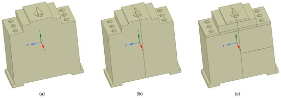
Figure 1.
Example of electrical component partitioning method. (a) Single-block division. (b) Two-block division. (c) Multi-block division.
3.2.2. An Optimization Strategy for Simulation Parameters of an Equivalent Model
The rational setting of simulation parameters for equivalent models of electrical components is crucial to ensuring the accuracy of simulation results. The main simulation parameters of equivalent models include the following: the division method of the equivalent model, the power loading location applied to the equivalent model, and the thermal conductivity assigned to the equivalent model. The technical route for determining the simulation parameters of equivalent models is generally as follows: First, obtain the temperature distribution data on the surface of a specific type of electrical component through temperature rise tests, including the distribution of the temperature field and specific temperature values; then, calculate the heat generation power of the electrical component based on the test parameters and use it as input to compute the thermal simulation results of the electrical component equivalent model; next, compare the test results with the simulation results: if there are significant discrepancies between the temperature values of temperature field in the simulation results and the test results, modify the equivalent model division method, power application location, and equivalent thermal conductivity until the simulation results match the measured results, finally, obtain the optimal simulation parameters for the equivalent model through iterative optimization.
From the above technical route, it can be seen that the process of determining the simulation parameters for the equivalent model of electrical components is essentially an optimization problem. Here, the optimization objective is to make the temperature distribution and values of the equivalent model as close as possible to the test results. The similarity of temperature distribution can be evaluated by the coefficient of determination in Equation (5), and the deviation of temperature values can be evaluated by the root mean square error (RMSE) in Equation (6). The decision variables are the simulation parameters to be determined for the equivalent model, namely the equivalent model division method, power loading location, and equivalent thermal conductivity. The constraint conditions mainly involve the optimizable range of variables, such as the number of division blocks n should not be excessively large, the number of feasible power loading locations m should not exceed n, and the equivalent thermal conductivity should be greater than 0. The specific process for optimizing the simulation parameters of the equivalent model is shown in Figure 2.
where denotes the number of sample points for verifying the equivalent model’s accuracy. When selecting comparative samples, it is crucial to ensure a uniform distribution across the electrical component’s outer surface. represents the simulation result at the i-th sample point; while is the measured value at the same point, determined through temperature rise experiments. The mean of all measured values across the sample points is indicated by .
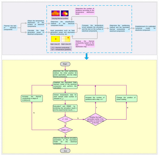
Figure 2.
Optimization strategy for equivalent model simulation parameters. * used for emphasis.
To improve iteration efficiency, this paper proposes a method for calculating the initial equivalent thermal conductivity, which can be used to determine the equivalent thermal conductivity of electrical components in the first iteration. The following assumptions are first made:
- (1)
- The electrical component is simplified as a cubic solid, with different lengths, widths, and heights for cubes of different component models.
- (2)
- The applied power is calculated based on the rated current and resistance, with the power loading location set at the center of the cube.
- (3)
- The maximum temperature on the front panel of the electrical component is estimated: for low-power components, the maximum temperature is assumed to be the same as the ambient temperature; for high-power components, the maximum temperature is the sum of the ambient temperature and the temperature rise limit (e.g., 60 K), and linear interpolation is used for components with intermediate power levels.
- (4)
- The temperature gradients in the three orthogonal directions are identical.
Based on assumptions (1)–(3), Equation (7) can be derived using the heat conduction formula:
where denotes the estimated maximum temperature of the electrical component’s front panel, which can be predicted according to Assumption (3); is the temperature at the center of the cubic solid; P represents the heat generation power of the electrical component; k is the equivalent thermal conductivity; and L is the length of the electrical component.
Based on Assumption (4), Equation (8) can be obtained:
where and denote the temperatures of the surfaces corresponding to the width and height, respectively; W and H represent the width and height of the electrical component, respectively.
According to the law of energy conservation, the heat dissipation of the electrical component is equal to its heat generation power:
where and represent the surface heat dissipation and heat dissipation area, respectively; h is the convective heat transfer coefficient, taking an empirical value of ; and is the room temperature.
3.2.3. Calculation Method of Electrical Component Heat Generation Power
During the temperature rise test of electrical components, heat transfer between wires and components can occur in either direction, as analyzed in Figure 3. To ensure the heat generation power applied to the component’s equivalent FEM matches reality and to guarantee component calibration accuracy, the impact of wires on the component’s temperature rise must be considered.
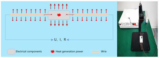
Figure 3.
System energy analysis.
According to the law of energy conservation, the actual heat-generation power of an electrical component can be calculated using Equation (11):
where , , and denote the actual heat-generation power of the electrical component, the total power, and the heat-dissipation power of the wire, respectively. When the electrical component is a circuit breaker, the total power can be calculated using Equation (12); when it is a relay/contact, the total power can be determined using Equation (13).
where and are the total circuit current and resistance, while and are the component’s coil voltage and resistance.
Since connecting wires have resistive losses and generate heat, and heat transfer occurs at the connection points, the wires play a crucial role in the thermal analysis of electrical components. The heat-dissipation power of the wires can be calculated using the following equation.
where S is the total surface area of the wire. and represent the average surface temperature of the wire and the ambient temperature, respectively. is the overall heat transfer coefficient of the wire surface, is the overall heat transfer coefficient for bare wire, is the thermal conductivity of the insulating material, is the radius of the wire with insulation, and is the radius of the bare wire.
The connecting wire, exposed to air, dissipates heat through convection and radiation. Therefore, the overall heat transfer coefficient for the bare wire consists of two components.
where is the overall heat transfer coefficient of the bare wire surface, and are the convective and radiative heat transfer coefficients, respectively. The convective and radiative heat transfer coefficients for the bare wire are calculated using Equations (17) and (18).
where d is the wire diameter, is the Stefan–Boltzmann constant, taken as . The emissivity is taken as 0.86. F is the shape factor, which is taken as 1 when calculating the radiation heat dissipation from the outer shell and the outer surface of the wire.
3.2.4. Validation of the Accuracy of the Equivalent Model Modeling Method
Taking the electrical component 3RV1021-1DA15 (Siemens AG of Germany, Beijing, China) as an example, a temperature rise experiment of the electrical component is carried out, and its wiring schematic diagram is shown in Figure 4. The letters ‘T’ and ‘L’ represent the main contact identification, ‘L’ represents the incoming end, and ‘T’ represents the outgoing end. Table 1 and Figure 5 present the test results of its surface temperature rise and the temperature rise contours. The ambient temperature in the test was 19 °C, the average temperature on the wire surface was , the circuit current was 3, A, and the total circuit steady-state resistance was .
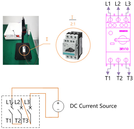
Figure 4.
Schematic diagram of the wiring for the temperature rise test of electrical components.

Table 1.
Temperature rise test results of 3RV1021-1DA15.
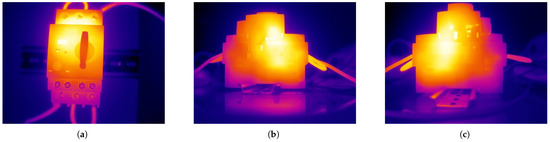
Figure 5.
Experimental results of temperature field distribution for electrical components. (a) Top enclosure. (b) Left enclosure. (c) Right enclosure.
Based on the modeling method for electrical component equivalent models in Section 3.2 and the optimization strategy in Figure 2, the partitioning, power loading positions, and equivalent thermal conductivity of the equivalent model were determined. Figure 6 and Table 2 compare the initial simulation results with experimental data. In the initial design, a single-block partitioning was used (see Figure 1a), and the equivalent thermal conductivity was calculated as in Section 3.2.2, yielding a value of . The comparison reveals significant discrepancies between the simulation and experimental results in both temperature distribution trends and key-point temperatures on the component’s outer surface.
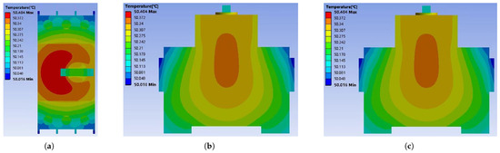
Figure 6.
Simulation results of temperature field distribution for electrical components (initial design). (a) Top enclosure. (b) Left enclosure. (c) Right enclosure.
Table 2.
Comparison of simulated and measured temperatures at key points (initial design).
Figure 7 and Table 3 present a comparison of the simulation results from the optimized equivalent model with experimental data. The equivalent model of component 3RV1021-1DA15 was partitioned into two sections (see Figure 1b for reference), and an equivalent thermal conductivity of was determined through iterative calculations. Figure 7 shows the temperature distribution contours from the simulation. The temperature field distribution on the outer surface of the component in the simulation aligns closely with the experimental results, exhibiting a consistent overall pattern. Table 3 compares the temperatures at selected key points, revealing that the simulation results deviate from the experimental data by no more than , with an average error of , indicating a satisfactory simulation outcome. This process validated the reliability of the modeling method for the equivalent model of the electrical component and the precision of the simulation.
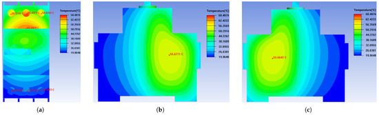
Figure 7.
Simulation results of temperature field distribution for electrical components (after optimization). (a) Top enclosure. (b) Left enclosure. (c) Right enclosure.
Table 3.
Comparison of simulated and measured temperatures at key points (after optimization)).
Based on the above approach, a comprehensive analysis was conducted on 52 common electrical components in the electrical cabinet of the CR400BF EMU (CRRC Tangshan Co., Ltd., Tangshan City, China). Their equivalent model parameters were determined, and corresponding models were built and integrated into a component library. Through parametric and modular mechanisms, this library offers basic units for rapidly constructing a multiphysics coupled finite element model of the cabinet. It strongly supports thermal analysis, fault prediction, and optimization of electrical cabinets across train models under various conditions.
3.3. Verification of the Accuracy of the Finite Element Model for Electrical Cabinet Temperature Rise
3.3.1. Actual Carriage Test
To verify the simulation method’s accuracy for electrical cabinets, on EMU temperature rise tests were conducted on the electrical cabinet of Carriage 02 in a CR400BF Fuxing-series EMU operating on the main line on 28 December 2024. This experimental testing equipment adopts a SmartMeter temperature detection recorder, which can collect temperature through external temperature sensors and transmit it in real time through a 4G network. The external sensor is a patch type temperature probe, which is attached to the surface of the measured point with high-temperature tape. The location of the measuring point and the testing site are shown in Figure 8.
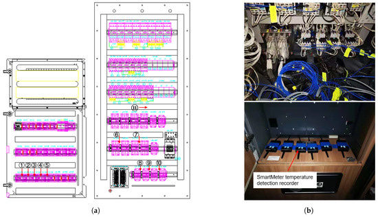
Figure 8.
Measurement location and testing site. (a) Measurement point location. (b) Testing site.
When conducting on-site testing, the first step is to stick the surface-mounted temperature probe. Then, place the SmartMeter temperature detection recorder on the outside of the cabinet, turn on automatic data transmission and set the data acquisition frequency (sampling frequency is 1 time/min), and finally close the cabinet door. The train runs normally and maintains the daily working status of the electrical cabinet, with a total collection time of 12 h. Extract the maximum temperature value of each temperature measurement point during the testing period and calculate the temperature rise. The experimental results are shown in Table 4.
Table 4.
On-site carriage test results of electrical cabinet.
3.3.2. Finite Element Calculation Model
Based on the calibrated equivalent model of electrical components, the ANSYS Workbench software (version 2019 R2) was used to partition the grid, set material parameters, load, and boundary conditions according to the three-dimensional geometric model of the electrical cabinet of the test object 02 car (as shown in Figure 9a) and the electrical component model and power consumption table (as shown in Table 5). The simulation model of the electrical cabinet is shown in Figure 9b. The specific settings of the finite element model are as follows:
- (1)
- Calculation domain and boundary setting: The calculation domain not only includes the electrical cabinet itself, but also extends to its surrounding air environment, used to simulate the effects of natural and forced convection. According to the actual installation conditions, the bottom of the electrical cabinet is in direct contact with the floor, and in the simulation, the bottom surface is set as an adiabatic boundary; there is a gap of about 80 mm between the electrical cabinet and the wall, and a space of 450 mm between the cabinet and the ceiling. The side and top air zones are set as solid wall boundaries to simulate heat reflection and spatial confinement effects; the entire computational domain ultimately forms a rectangular enclosed space containing the cabinet and surrounding air.
- (2)
- The fan component simulates the forced air cooling process inside the electrical cabinet, and the performance parameters of the fan are input based on the characteristic curve provided by the manufacturer. Set the fan type to Intake. The air inlet and outlet are defined by Grille and set as inlet grille and opening grille, respectively. The ambient temperature is uniformly set at C.
- (3)
- Grid generation strategy: Icepak adopts an automatic grid partitioning strategy, combined with the complex geometric structure of electrical cabinets, to locally refine key areas (such as main thermoelectric devices, near air ducts, etc.), while maintaining coarser background grids in other areas to balance computational accuracy and efficiency. Grid independence is compared and analyzed through three different numbers of grid models.
- (4)
- Turbulence model selection: This article uses the standard turbulence model for solving, which has good computational stability and adaptability in the Icepak environment and is suitable for simulating hot air flow fields under fan drive.
- (5)
- Convection parameter settings: Enable the advanced forced convection solver option in Icepak to enhance the ability to solve airflow in ducts.

Figure 9.
Electrical cabinet model in carriage 02. (a) 3D model of electrical cabinet in carriage 02. (b) Finite element model of electrical cabinet in carriage 02. (c) Simulation results of electrical cabinet in carriage 02.
Table 5.
Electrical component models and power dissipation (All components are sourced from the same manufacturer, Siemens AG of Germany, Beijing, China).
Table 5.
Electrical component models and power dissipation (All components are sourced from the same manufacturer, Siemens AG of Germany, Beijing, China).
| Item | Model of Electrical Component | Power | Operational Status |
| 1 | Breaker 3RV1031-4EA10 | Rated power consumption: 17.7 W | On |
| 2 | Breaker 3RV1021-1HA15 | Rated power consumption: 4.2 W | On |
| 3 | Relay 3TX70051LN00 | Rated power consumption: 1.2 W | On |
| 4 | Relay 3RP15-05-2BW30 | Rated power consumption: 0.3 W | On |
| 5 | Relay 3UG4511-2AP20 | Rated power consumption: 4 W | On |
| 6 | Relay 3RH1122-2KF40-0LA0 | Rated power consumption: 1.8 W | On |
| 7 | Contactor 3RT1025-3KF44-0LA0 | Rated power consumption: 4.6 W | On |
| 8 | Contactor 3RT1017-2KF42-0LA0 | Rated power consumption: 3.0 W | On |
| 9 | Contactor 3RT1034-3KF44-0LA0 | Rated power consumption: 7.3 W | On |
| 10 | Fan 7210 N-70181 | Air flow: 6 m3/min; Head pressure: 150 Pa | On |
| 11 | Air outlet size | Diameter: 68.6 mm | On |
3.3.3. Analysis of Temperature Field Simulation Results
Thermal simulation analysis based on a finite element model shows the temperature distribution in the electrical cabinet during traction operation, as depicted in Figure 9c. The cabinet exhibits higher temperatures at the top and center, and lower temperatures at the bottom and sides, aligning with real-world conditions. Data extracted from simulation test points and compared with actual measurements (Table 6 and Figure 10) reveal consistent trends in cabinet temperature and temperature rise. The maximum error for electrical component temperatures is within , and the average error is below . This confirms the effectiveness of the simulation method proposed in this paper.
Table 6.
Comparison of simulation and actual carriage test data.
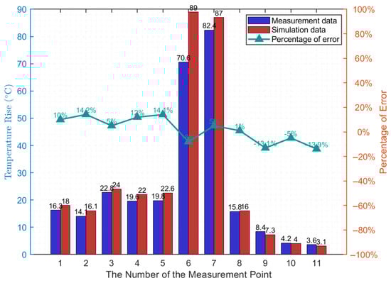
Figure 10.
Comparison of simulated and actual temperature rise values.
3.3.4. Analysis of Fluid Flow Field Simulation Results
As depicted in Figure 11, vector plots illustrate velocity distributions across three sections of the electrical cabinet’s 3D flow field. Figure 11a shows the xy-plane at the z-axis center, Figure 11b the yz-plane at the x-axis center, and Figure 11c the xz-plane at the y-axis center. These visualizations reveal fluid flow direction and velocity magnitude.
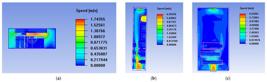
Figure 11.
Electrical cabinet sectional flow velocity vector diagram. (a) Top view. (b) Side view. (c) Front view.
Hot air inside the cabinet is expelled via the ceiling-mounted ventilation fan, while cool external air enters through lower inlets, facilitating efficient cooling. Maximum air velocity within the cabinet reaches m/s. According to Figure 11, it can be seen that the air flow velocity inside the cabinet is the highest at the air inlet, which is also due to the dense arrangement of electrical components here. Next is the air outlet located at the top, and the flow rate in the middle of the cabinet is relatively low due to the large space. It can be seen from this that there is a significant unevenness in the distribution of flow velocity field inside the electrical cabinet.
Based on the comprehensive flow field and temperature field, it can be concluded that the high flow velocity and low airflow temperature near the air inlet are beneficial for enhancing the cooling effect on electrical components; the flow velocity in the upper region is relatively low, and the airflow continuously absorbs heat from electrical components during its ascent, resulting in a gradual increase in temperature. Therefore, placing electrical components with higher temperature rise in the lower part of the electrical cabinet is more conducive to heat dissipation, higher airflow velocity, and lower intake temperature, which can significantly improve heat dissipation efficiency, while the upper area is more suitable for placing devices with lower heat generation.
4. Thermal Optimization Design of Electrical Cabinet
From the simulation results in Section 3.3, under traction operation conditions, the temperature rise of multiple electrical components in the EMU cabinet exceeds the C limit. The first-row circuit breaker 3RV1031-4EA10 on the rear panel reaches C, a C rise. This high temperature rise can disrupt normal operations. Therefore, analyzing the factors affecting component temperature rise and developing cost-effective optimization measures is essential to meet the temperature rise limits. This chapter uses the extreme condition of all components operating at full power.
4.1. Analysis of the Impact of Installation Gap on Temperature Rise
By adjusting the 3D model to increase the installation gap between the first-row circuit breakers 3RV1031-4EA10 on the rear panel, five comparative conditions with gaps of 0 mm, 2 mm, 4 mm, 6 mm, and 10 mm were set. The aim was to study the temperature rise in the electrical cabinet when all components operate at full power under extreme conditions. The simulation results are shown in Figure 12.
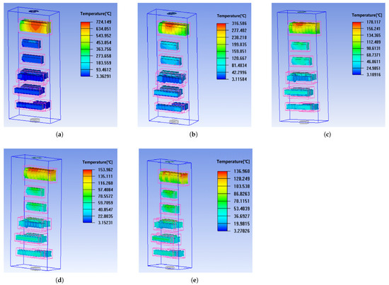
Figure 12.
Temperature field contour map of the electrical cabinet under different installation gaps. (a) 0 mm. (b) 2 mm. (c) 4 mm. (d) 6 mm. (e) 10 mm.
From the optimized simulation results of the electrical cabinet in Figure 12 and Figure 13, it can be seen that, by increasing the installation gap to 10 mm, the maximum temperature of the electrical components decreases from C to C, showing a significant temperature reduction effect. When the installation gap increases from 0 mm to 2 mm, the maximum temperature of the electrical components drops from C to C, a reduction of , indicating a marked cooling effect. Further increasing the installation gap to 4 mm reduces the maximum temperature of the electrical components to C, a reduction of , which is also a good cooling effect, but the trend of weakening has already appeared. Increasing the installation gap further to 6 mm and 10 mm reduces the maximum temperature of the electrical components to C and C, respectively, with reduction rates of and . It can be seen that further increasing the installation gap cannot effectively reduce the temperature. To maximize the use of cabinet space, an installation gap of 4–6 mm is recommended.
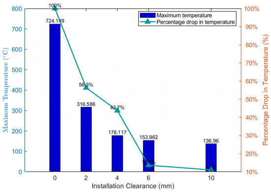
Figure 13.
Installation gap maximum temperature map.
4.2. Analysis of the Impact of Installation Position on Temperature Rise
Based on the finite element model of an electrical cabinet with an installation gap of 4mm, the first-row circuit breakers with high heat generation were swapped with the third and sixth-row components, respectively, by adjusting the 3D model. Figure 14 shows the comparison of different installation positions and their impact on temperature rise.
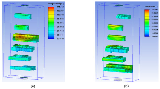
Figure 14.
Temperature field distribution contours for different installation positions of electrical components. (a) Swap the first-row and third-row electrical component. (b) Swap the first-row and sixth-row electrical component.
As seen in Figure 12c and Figure 14a, swapping the first-row components with the third-row ones lowers the highest component temperature from C to C (a drop). Swapping with the sixth-row components reduces it to C (a drop). Installation position significantly impacts component temperature rise. Per the temperature and flow field analyses in Section 3.3.3 and 3.3.4, the third row has low flow velocity, while the sixth row has the highest. Cold air enters from the bottom inlet, heats up via thermal exchange with components, and has a higher temperature near the top outlet. Better heat dissipation occurs at larger temperature differences, so areas closer to the inlet and with higher flow velocity have better cooling.
4.3. Analysis of the Impact of Ventilation Airflow on Temperature Rise
As per the analysis in Section 4.2, fluid velocity may influence the temperature rise of electrical components. With a constant heat-dissipation gap of 4 mm, the impact of ventilation airflow rate on temperature rise was studied by comparing rates from 6 to 18 m3/min. Figure 15 shows the simulation results. When the airflow rate rose from 6 m3/min to 10, 14, and 18 m3/min, the temperature dropped by , , and respectively. Thus, temperature rise decreases with increasing ventilation airflow. However, higher airflow rates also lead to greater power consumption and noise levels.
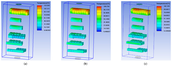
Figure 15.
Temperature field distribution contours at different ventilation airflow rates. (a) 10 m3/min. (b) 14 m3/min. (c) 18 m3/min.
4.4. Analysis of the Impact of Inlet Shape and Dimensions on Temperature Rise
Increasing the ventilation airflow can reduce the temperature rise to some extent, but it also leads to higher power consumption and noise levels. Optimizing the inlet shape can avoid these issues. Therefore, this section focuses on analyzing the impact of the inlet shape and dimensions on the temperature rise in Figure 16. As shown in Figure 16a, the analysis keeps the inlet area constant. When the inlet shape changes from a circle to a square (aspect ratio of 1:1), there is no significant change in the temperature rise of the electrical components. However, as the aspect ratio increases to 2:1, 3:1, and 4:1, the temperature first decreases and then increases. The minimum temperature occurs at an aspect ratio of 2:1, where the temperature rise decreases by approximately . This indicates that, when the inlet area remains constant, the shape and dimensions of the inlet can still affect the temperature rise.
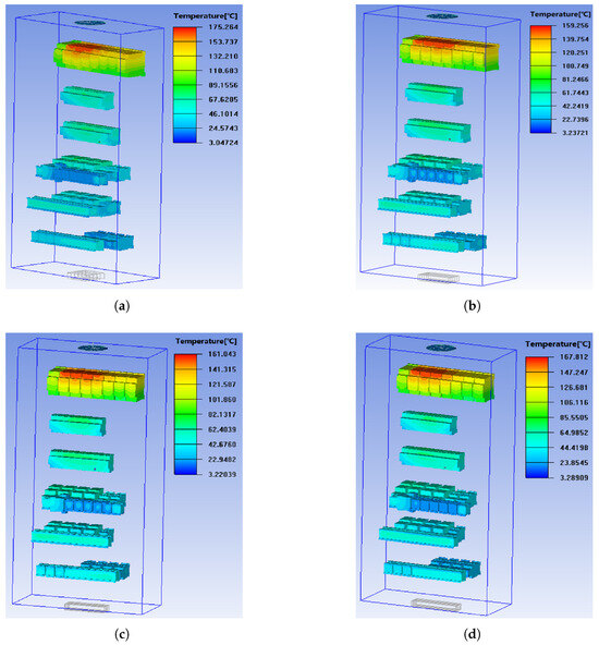
Figure 16.
Temperature field distribution contours for rectangular inlets with different aspect ratios. (a) Aspect ratio of 1:1. (b) Aspect ratio of 2:1. (c) Aspect ratio of 3:1. (d) Aspect ratio of 4:1.
4.5. Electrical Cabinet Optimization Design
As per the thermal analysis in Section 4.1, Section 4.2, Section 4.3 and Section 4.4, factors like installation gap, position, ventilation airflow, and inlet shape affect the electrical cabinet’s temperature rise. Parametric studies have revealed their specific impact patterns. To ensure electrical components’ temperature rise does not exceed C under extreme conditions, the following optimizations are performed:
- (1)
- Set a 4 mm gap for the first-row breakers with high heat generation and swap their installation positions with the sixth-row components.
- (2)
- Change the inlet opening to a rectangle with a 2:1 aspect ratio.
- (3)
- Increase ventilation airflow to cap the components’ temperature rise at C.
Figure 17 shows that, when ventilation airflow reaches 10 m3/min, the temperature rise meets the limit under extreme conditions. Thus, for EMU trains, ventilation airflow can be raised to 10 m3/min when entering extreme full-power mode, and dynamically reduced in other conditions to cut power consumption.
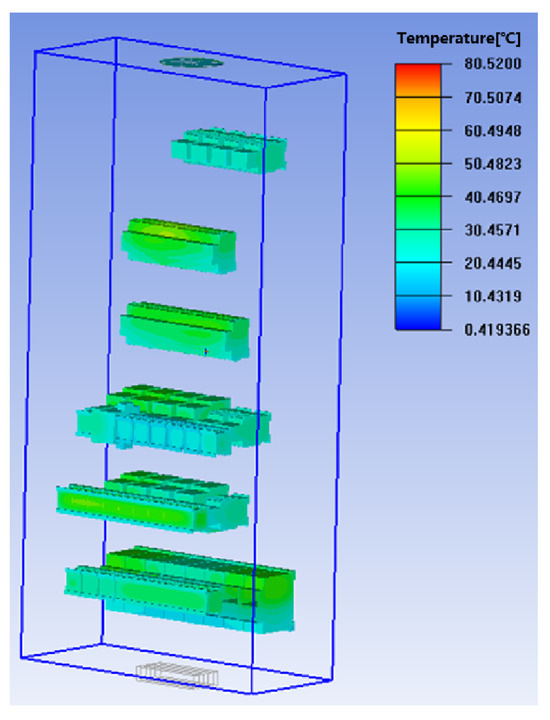
Figure 17.
Temperature field distribution contour after electrical cabinet optimization.
5. Conclusions
This paper presents a temperature field simulation method for EMU electrical cabinets, whose accuracy is verified by comparing with real-carriage test results. Based on this modeling method, the impacts of different influencing factors on the temperature rise of electrical components are analyzed, and an optimized design scheme is finally proposed. The main conclusions of this paper are as follows:
- (1)
- A modeling method for equivalent models of electrical components is proposed. Aiming at the complex thermal management issues caused by high-density integration of heterogeneous components, dynamic thermal loads under multi-operating conditions, and topological configuration changes across multiple carriage types in EMU electrical cabinets, a dual-metric-driven finite element model calibration method is developed based on the ANSYS Workbench platform. By constructing a multi-objective optimization function with the coefficient of determination and root mean square error () as core indices, the parameter calibration of equivalent models for 52 common types of electrical components in EMU electrical cabinets is systematically completed. Comparison with test results shows that this method can not only simulate the external temperature field distribution of electrical components but also accurately predict their temperature values, with an average error within .
- (2)
- A modeling method for multiphysics coupled finite element models of electrical cabinets is presented. Based on the equivalent library of electrical components, combined with different layouts and operating conditions of the electrical cabinet, differentiated power losses are loaded to establish a thermal–fluid field collaborative model. Comparison with real-carriage test results shows that the simulation results can accurately predict the temperature rise of different electrical components, with a maximum error within and an average error within , meeting the requirements for engineering applications.
- (3)
- Through studying the influence of different factors on the temperature rise of electrical components, it was found that, the smaller the installation gap, the higher the temperature rise of electrical components. However, a large installation gap can affect the compactness of the cabinet. It is recommended that the installation gap of electrical components with high temperature rise be between 4 and 6 mm. The larger the fan exhaust volume, the higher the heat dissipation effect of the cabinet, but it will also bring greater power consumption and noise. It is recommended to dynamically adjust the fan exhaust volume according to the operating conditions of the high-speed train. The installation position of electrical components also has a significant impact on their heat dissipation effect. Electrical components with higher temperature rise can be installed near the air inlet; the recommended shape for the air inlet is a rectangle with a length-to-width ratio of 2:1.
- (4)
- An optimized design scheme is proposed. It is ensured that, under extreme operating conditions, the temperature rise of electrical components within the electrical cabinet does not exceed the limit of C.
The research results provide a standardized modeling framework and data support for the optimized design of thermal management systems and thermal fault prediction in EMU electrical cabinets, contributing to improving the thermal reliability of electrical cabinets and the operational stability of the system.
Author Contributions
Conceptualization, Y.W. and C.X.; Methodology, Y.W. and C.X.; Software, Y.W. and S.C.; Validation, Y.W. and S.C.; Writing—Original Draft Preparation, Y.W. and C.X.; Writing—Review Editing, Z.T.; Supervision, Z.D.; Resources, C.X.; Project Administration, C.X.; Data Curation, Z.D. and Z.T. All authors have read and agreed to the published version of the manuscript.
Funding
This work was supported by Guangxi Key Laboratory of Automatic Detecting Technology and Instruments (YQ23106), the Special Funds of the National Natural Science Foundation of China (No.62341304), the National Natural Science Foundation of China (No.42263003), the Guangxi Science and Technology Base and Specialized Talents (No.2021AC19451), and Undergraduate Innovation Training Program of Guilin University of Electronic Technology (No.202410595001).
Data Availability Statement
The original contributions presented in the study are included in the article, further inquiries can be directed to the corresponding author.
Conflicts of Interest
The authors declare no conflicts of interest.
References
- Qi, Y.; Zhou, L. The fuxing: The China standard EMU. Engineering 2020, 6, 227–233. [Google Scholar] [CrossRef]
- Zhao, H.; Huang, Z.; Mei, Y. High-speed EMU TCMS design and LCC technology research. Engineering 2017, 3, 122–129. [Google Scholar] [CrossRef]
- Lu, C.; Zhang, B.; Zhao, H. CR-Fuxing high-speed EMU series. Front. Eng. Manag. 2023, 10, 742–748. [Google Scholar] [CrossRef]
- Zhao, H.; Liang, J.; Liu, C. High-speed EMUs: Characteristics of technological development and trends. Engineering 2020, 6, 234–244. [Google Scholar] [CrossRef]
- Li, R.; Yang, W.; Liang, H. Multi-physics finite element model of relay contact resistance and temperature rise considering multi-scale and 3D fractal surface. IEEE Access 2020, 8, 122241–122250. [Google Scholar] [CrossRef]
- Rodríguez, A.; Pérez-Artieda, G.; Beisti, I.; Astrain, D.; Martínez, A. Influence of temperature and aging on the thermal contact resistance in thermoelectric devices. J. Electron. Mater. 2020, 49, 2943–2953. [Google Scholar] [CrossRef]
- Ye, J.; Lyu, K.; Liu, G.; Qiu, J. Study on the intermittent fault mechanism of electromagnetic relay under complex environmental stress. In Proceedings of the PHM Society Asia-Pacific Conference, Tokyo, Japan, 11–14 September 2023; Volume 4. [Google Scholar]
- Lakshminarayanan, V.; Sriraam, N. The effect of temperature on the reliability of electronic components. In Proceedings of the 2014 IEEE international conference on electronics, computing and communication technologies (CONECCT), Bangalore, India, 6–7 January 2014; IEEE: New York, NY, USA, 2014; pp. 1–6. [Google Scholar]
- Almubarak, A.A. The effects of heat on electronic components. Int. J. Eng. Res. Appl. 2017, 7, 52–57. [Google Scholar] [CrossRef]
- Wang, W.; Sun, Y.; Sun, P.; Song, Y.; Lin, X.; Zhao, H.; Zhang, J. Development of A Temperature Rise Test System Based on The New Technology of Switching Power Supply Control. In Proceedings of the 2021 13th International Conference on Measuring Technology and Mechatronics Automation (ICMTMA), Beihai, China, 16–17 January 2021; IEEE: New York, NY, USA, 2021; pp. 409–413. [Google Scholar]
- Zhang, X.; Gockenbach, E.; Wasserberg, V.; Borsi, H. Estimation of the lifetime of the electrical components in distribution networks. IEEE Trans. Power Deliv. 2006, 22, 515–522. [Google Scholar] [CrossRef]
- Szulborski, M.; Łapczyński, S.; Kolimas, Ł. Thermal analysis of heat distribution in busbars during rated current flow in low-voltage industrial switchgear. Energies 2021, 14, 2427. [Google Scholar] [CrossRef]
- Haag, D.; Stergiaropoulos, K. Fast thermodynamic simulation of electrical control cabinets via thermal resistor networks. J. Phys. Conf. Ser. 2024, 2766, 012209. [Google Scholar] [CrossRef]
- Tang, N.; Xu, H.; Bai, X.; Li, X. Analysis of thermal characteristics of switch cabinet with multi-physics field coupling method. In Proceedings of the 2020 IEEE 66th Holm Conference on Electrical Contacts and Intensive Course (HLM), San Antonio, TX, USA, 30 September–7 October 2020; IEEE: New York, NY, USA, 2020; pp. 28–34. [Google Scholar]
- Wang, Z.; Wang, R.; Yan, C.; Wang, L.; Wu, J. Heat Dissipation improvement of medium-voltage switch-gear: Simulation study and experimental validation. In Proceedings of the 2019 5th International Conference on Electric Power Equipment-Switching Technology (ICEPE-ST), Kitakyushu, Japan, 13–16 October 2019; IEEE: New York, NY, USA, 2019; pp. 522–526. [Google Scholar]
- Zheng, W.; Jia, X.; Zhou, Z.; Yang, J.; Wang, Q. Multi-physical field coupling simulation and thermal design of 10 kV-KYN28A high-current switchgear. Therm. Sci. Eng. Prog. 2023, 43, 101954. [Google Scholar] [CrossRef]
- Zheng, W.; Si, W.; Fu, C.; Ju, D.; Chen, C.; Qian, S.; Yang, J.; Wang, Q. Multi-physics coupling simulation of heat transfer and thermal design for high voltage switchgear busbar room. Chem. Eng. Trans. 2022, 94, 193–198. [Google Scholar]
- Son, M.; Kang, H.; Lee, S.; Ahn, G.; Kim, Y. The study of temperature rise in low voltage switchgear about cooling system. In Proceedings of the 2017 4th International Conference on Electric Power Equipment-Switching Technology (ICEPE-ST), Xi’an, China, 22–25 October 2017; IEEE: New York, NY, USA, 2017; pp. 218–220. [Google Scholar]
- Yao, Y.; Ouyang, X.; Zeng, G.; Tang, Q.; Ma, W. Research on modularizing design of 10 kV switchgear with line outlet for live maintenance. Energy Rep. 2021, 7, 10–16. [Google Scholar] [CrossRef]
- Li, P.; Jia, T.; Zhang, Z.; Li, W.; Gao, Y.; Zheng, N. Simulation analysis of electromagnetic-temperature field coupling of medium voltage switchgear based on finite element method. J. Phys. Conf. Ser. 2020, 1639, 012032. [Google Scholar] [CrossRef]
- Krajewski, W.; Krasuski, K.; Błażejczyk, T. Some aspects of medium voltage switchgear designing with aid of numerical analysis. IET Sci. Meas. Technol. 2020, 14, 651–664. [Google Scholar] [CrossRef]
- Ruan, J.; Wu, Y.; Li, P.; Long, M.; Gong, Y. Optimum methods of thermal-fluid numerical simulation for switchgear. IEEE Access 2019, 7, 32735–32744. [Google Scholar] [CrossRef]
- Alsumaidaee, Y.A.M.; Yaw, C.T.; Koh, S.P.; Tiong, S.K.; Chen, C.P.; Ali, K. Review of medium-voltage switchgear fault detection in a condition-based monitoring system by using deep learning. Energies 2022, 15, 6762. [Google Scholar] [CrossRef]
- You, Y.; Lin, J.; Dai, D.; Sang, Z. 10 KV Switchgear Temperature Field Analysis and Product Structure Optimization Research. In Proceedings of the 2024 7th International Conference on Electric Power Equipment-Switching Technology (ICEPE-ST), Xiamen, China, 10–13 November 2024; IEEE: New York, NY, USA, 2024; pp. 368–374. [Google Scholar]
Disclaimer/Publisher’s Note: The statements, opinions and data contained in all publications are solely those of the individual author(s) and contributor(s) and not of MDPI and/or the editor(s). MDPI and/or the editor(s) disclaim responsibility for any injury to people or property resulting from any ideas, methods, instructions or products referred to in the content. |
© 2025 by the authors. Licensee MDPI, Basel, Switzerland. This article is an open access article distributed under the terms and conditions of the Creative Commons Attribution (CC BY) license (https://creativecommons.org/licenses/by/4.0/).