Forecasting Power Quality Parameters Using Decision Tree and KNN Algorithms in a Small-Scale Off-Grid Platform

Abstract

This article presents the results of a performance comparison of four forecasting methods for prediction of electric power quality parameters (PQPs) in small-scale off-grid environments. Forecasting PQPs is crucial in supporting smart grid control and planning strategies by enabling better management, enhancing system reliability, and optimizing the integration of distributed energy resources. The following methods were compared: Bagging Decision Tree (BGDT), Boosting Decision Tree (BODT), and the K-Nearest Neighbor (KNN) algorithm with $k-5$ and $k-10$ nearest neighbors considered by the algorithm when making a prediction. The main goal of this study is to find a relation between the input variables (weather conditions, first and second back steps of PQPs, and consumed power of home appliances) and the power quality parameters as target outputs. The studied PQPs are the amplitude of power voltage (U), Voltage Total Harmonic Distortion ($TH{D}_u$), Current Total Harmonic Distortion ($TH{D}_i$), Power Factor ($PF$), and Power Load ($PL$). The Root Mean Square Error (RMSE) was used to evaluate the forecasting results. BGDT accomplished better forecasting results for $TH{D}_u$, $TH{D}_i$, and $PF$. Only BODT obtained a good forecasting result for $PL$. The KNN (k = 5) algorithm obtained a good result for $PF$ prediction. The KNN (k = 10) algorithm predicted acceptable results for U and $PF$. The computation time was considered, and the KNN algorithm took a shorter time than ensemble decision trees.

1. Introduction

The production of electricity using traditional methods of processing fossil and synthetic fuels contributes to high levels of pollution of the Earth’s atmosphere and causes a noticeable increase in the incidence of civilizational diseases such as cancer [1]. Currently, to reduce air pollution and CO₂ emissions, renewable energy sources are used to generate electricity. However, to deal with the instability of these power sources, due to the reliance on weather, smart control systems are needed to manage power generation and ensure satisfactory quality, especially in off-grid systems. The ongoing challenge is to design and apply a smart grid that can operate an off-grid power system under weather fluctuations in real time. Many different types of forecasting models have been developed, e.g., in [2], a fuzzy model was proposed using particle swarm optimization (PSO) to forecast solar and wind power generation. Another study applied a novel Bayesian ensembling model for wind power prediction [3]. In [4], an ANN was used to forecast wind speed. In [5], an optimized deep learning-based long short-term memory (LSTM) model was applied for power generation and consumption forecasting. The advantages of the model proposed in this study are outlined as follows: (1) The model uses the steps of each target output, and (2) the dataset was published for free. Moreover, the authors of [6] used an unconventional strategy for estimating sustainable energy output using a Neural Network (NN) and Convolutional Neural Network (CNN) to build a framework that can precisely predict offshore wind and PV energy production in the short term. In this respect, a power quality parameter forecasting process plays a vital role in smart grids, as it helps to generate power within satisfactory limits from renewable energy sources. Among numerous PQPs that define the quality of the power, the most important are the power frequency, total harmonic distortion of voltage ($TH{D}_u$) [7], total harmonic distortion of current ($TH{D}_i$), short-term flicker severity ($P_{st}$), and amplitude of the power voltage (U).

In a small-scale off-grid system, the power quality parameters (PQPs) should be forecasted to determine their future values according to weather conditions and home appliance operations. Once PQPs are predicted successfully, the next task is to reschedule the run time of the home appliances to an appropriate time, which should ensure a balance between generating power from renewable sources and power demand. The forecasted PQPs need to be constantly compared to standard values, not only to reschedule the load to meet the availability of the generated power but also to avoid damage to users’ devices. For example, Zjavka applied and compared three methods for PQPs in [8] and combined machine learning and regression models in [9]. Vantuch et al. used a random decision forest optimized by multi-objective optimization [10]. Stuchly et al. tested an ANN with a backpropagation learning algorithm [11]. Jahan et al. investigated a standard regression tree [12,13], linear regression, interaction linear regression, an ANN, quadratic linear regression, pure quadratic linear regression, bagging DT, and boosting DT [14]. In Indonesia [15], researchers applied Random Forest (RF) and a Poly-Exponential (PE) model to forecast power load and power quality. The results proved that the model requires fewer samples and yields a precise prediction. Quantile Regression (QR) models were applied with Principal Component Analysis (PCA) for forecasting of the power quality index level [16]. PCA was used for dimension reduction, and the numerical results confirmed that the model is suitable for PQ forecasting for both comprehensive indices and individual components. A forecasting system to predict voltage deviation was investigated in [17]. The proposed approach combines the following techniques: PCA for dimension reduction to reduce the input data dimension, affinity propagation to cluster the input data, and a BP neural network to estimate the voltage deviation. The model achieved good forecasting results compared with others.

As a practical application, the authors of [18] used data from a small number of smart meters to predict the voltage total harmonic distortion ($TH{D}_u$) for low-voltage busbars of residential distribution feeders. The technique gives the system operators access to pertinent power quality indicators by using the current monitoring infrastructure. In the work, several voltage total harmonic distortion forecasting techniques, including artificial neural networks, were evaluated. In [19], advanced Fuzzy Time Series (FTS) were applied for prediction of power quality events.

The experiment focused on interruptions and voltage sag forecasting. The study proved that the FTS algorithm fits power events, especially in the case of the non-ferrous metal industry. Research reported in [20] used a decision tree to predict the following power parameters: the disturbances considered as Earth faults, rapid voltage changes, and voltage dips. Another study [21] presented a real-time classification system for detection of power quality events, such as transient, sag, swell, interruption, or flicker events. The proposed identification and classification of power quality disruptions were based on machine learning and a hybrid deep learning approach. The authors compared the results of the XGBR, CatBoostR, LGBMR, and LSTM models with the those of the proposed Boosting CNN SOS. Yet another article [22] presented a more in-depth analysis of classification compared to the previously discussed publication. Here, the authors proposed a method for classifying power quality disturbance signals based on Segmented and Modified S-Transform (SMST), Multiclass Support Vector Machine (MSVM), and Deep Convolutional Neural Network (DCNN) models. This method uses frequency segmentation with various adjustable parameters as a function of a Gaussian window. The developed method made it possible to achieve accurate and effective extraction of features of various disturbances. The results show that the proposed method outperforms several state-of-the-art algorithms in classifying power quality disturbances at different noise levels. The authors of [23] proposed two different approaches for supervising selected electrical disturbances in low-voltage networks, such as voltage notch, voltage sag, voltage swell, harmonic disturbances, and interruption. The two approaches correspond to the classification of the frequency-domain voltage signals using machine learning techniques. The first technique uses Fourier transform (FT) to classify the corresponding disturbance classes through a Multilayer Neural Network with Multivalued Neurons (MLMVN).

The second method allows for the use of a Convolutional Neural Network (CNN) and Short-Time Fourier Transform (STFT) with each layer of 2D convolutions for dimensionality reduction and feature extraction. It should be mentioned that both of the aforementioned methods are characterized by high effectiveness. In [24], a model designed to forecast and classify the power quality disturbances was presented.

The latest encoder–decoder model was used as a forecasting system, with a hybrid convolutional neural network–long short-term memory (LSTM) model as the classifier model. Quantile Regression Averaging (QRA) was applied for short-term nodal voltage forecasting in [25]. The model was compared with three others, and the results confirmed that QRA achieves better performance than the other models. A forecasting method based on a Long short-term memory network for the forecast of power voltage and current was proposed in [26]. The system is not needed for the data processing stage, including feature extraction or selection, and the system was found to be robust and achieved good results for voltage and current forecasting. In [27], a deep learning method long short-term memory was investigated for voltage harmonics prediction in a wind turbine. The model was constructed in two steps: feature extraction using window segmentation and LSTM for forecasting. The authors concluded that the designed model is effective for forecasting voltage harmonics in power systems. In [28], a multilayer perceptron neural network (MLPNN) was applied for the forecasting of the harmonic distortion of current ($TH{D}_i$) in a system where photovoltaic cells were used. In such a solution, six different models of MLPNN with varying numbers of hidden layers and input parameters were tested. In general, all designed models achieved good forecasting accuracy. In [29], a long short-term memory model was presented for very short-term power frequency forecasting. The model was trainedusing four input variables: the previous frequency and power load, the day of the week, and the hour of the day. The study demonstrated the effectiveness of the designed methodology. A hidden Markov model with weather conditions was used to forecast disturbance events in power quality (PQ) in [30]. The system achieved better forecast accuracy compared to other traditional forecasting techniques. A similar solution was used by the authors of [31], where a hidden Markov model used the numerical weather prediction (NWP) in order to forecast the PV power production. In another solution for a microgrid purpose, an approach based on an artificial neural network was proposed to estimate the power voltage and total harmonic distortion (THD) [32].

The system was tested for four different cases, and the results proved that the model estimated the voltage and the THD worked successfully. In [33], machine learning methods were used to predict the following parameters: voltage dips, ground faults, rapid voltage changes, and interruptions. The best forecasting accuracy was achieved when using the random forest model, which achieved better performance than the other models. In [34], a short-term forecasting system based on machine learning techniques was proposed. The model was designed to predict voltage, frequency, and harmonic distortions. Four models were compared: XGBoost Regressor, two dense neural network models, and LSTM.

In [35], a VMD-XGBTCN method for power voltage prediction was proposed. This method was constructed using variable modal decomposition (VMD) for voltage signal decomposition. Then, feature selection was applied using Extreme Gradient Boosting (XGBoost) and a Temporal Convolutional Network (TCN) for voltage prediction. The designed system exhibited a slight error in voltage forecasting compared to the others, but it also offered better forecasting performance. Voltage instability prediction in a power system based on a Recurrent Neural Network (RNN) trained by Particle Swarm Optimization (PSO) was proposed in [36]. The test results proved the validity of the model. Researchers applied the Grey Wolf Optimizer with the Least Square Support Vector (GWO-LSSVM) to predict the Total Harmonic Distortion (THD) [37]. The performance of the studied model was compared with that of two other forecasting systems: the Standard Least Square Support Vector Machine (LSSVM) and Particle Swarm Optimization. A nonlinear autoregressive network was applied, combined with the Least Square Support Vector Machine (PSO-LSSVM). The forecasting accuracy of the designed model exceeds that of other compared models. The authors of [38] presented neuro-fuzzy modeling, which was applied for current total harmonic distortion ($TH{D}_i$) prediction appearing in the medium voltage range. The results of the designed system can be used for the filtering of the $TH{D}_i$ in the power supply.

The authors of [39] applied a nonlinear autoregressive network for the forecasting of the total harmonic distortion of voltage and current. The system was tested for three cases of nonlinear loads in three-phase networks. The results were evaluated and compared with the results of two other neural networks.

In [40], two algorithms, namely correlation kernel regression and the autoregressive moving average models, were used to forecast the frequency of signals, and the system was tested on three power grids. The experimental outcome proved the efficiency of the suggested models in voltage signal forecasting. Combining an Improved System Frequency Response (ISFR) model with a Long Short-Term Memory (LSTM) network for power frequency prediction was suggested in [41]. ISFR was used to generate the features; then, these features were fed to an LSTM to fit a relationship between the input features and the frequency response. The system was tested for the IEEE 39-bus system; the experimental results demonstrated that the designed model achieves better forecasting results than traditional systems. A neural network with a maximum information coefficient was applied in [42] for power frequency forecasting. The maximum information coefficient was used to extract features from the factors relevant to the power frequency; then, the neural network was used to predict the frequency. The model was validated using a historical power-grid dataset, and the results confirmed the prediction accuracy of the designed example.

Another study repored in [43] used an LSTM recurrent neural network for prediction of nonlinear power voltage. The research concluded that the system can fit the power voltage perfectly and achieves improved effectiveness and forecasting accuracy. A Generalized Regression Neural Network (GRNN), optimized by the Mind Evolution Algorithm (MEA) was tested in [44] to predict $TH{D}_i$ caused by LED lamps. The AdaBoost algorithm was used to combine several MEA-GRNN singles to improve the model’s prediction accuracy. The effectiveness of the model was compared with that of a BP neural network and a GRNN, and the prediction accuracy of the designed model reached 95.48%. In China, a study tested a hybrid model for short-term power load forecasting [45]. The system was built using adaptive mode decomposition and an improved least squares support vector machine. The simulation results confirmed the system’s effectiveness when compared with other existing models.

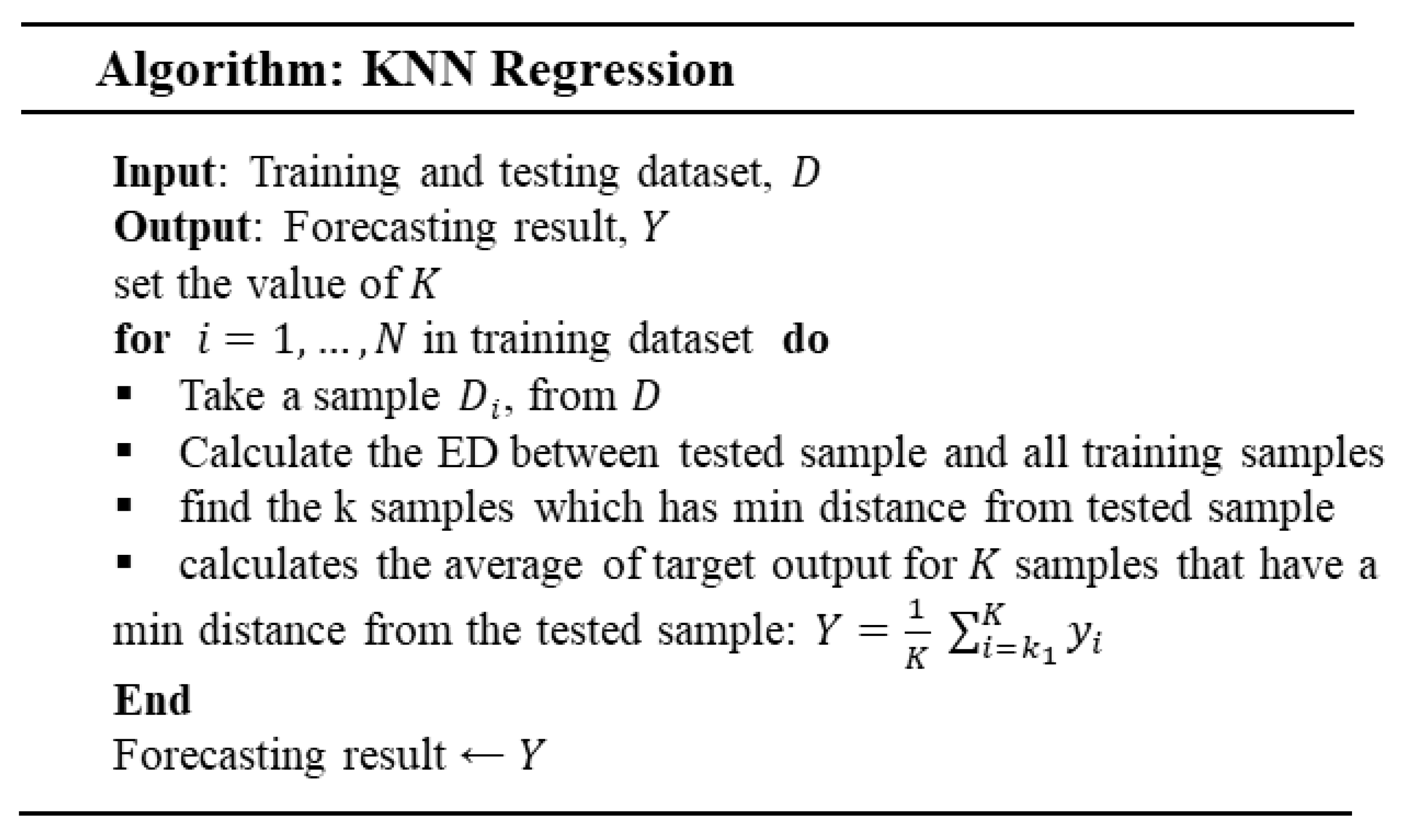
It is worth mentioning that KNN regression is a non-parametric technique in machine learning. This algorithm functions by calculating the distance between data points and selecting the k data points with the shortest distance, and the final output is the average of their outputs. The BGDT regression tree, which divides the original dataset into subsets and is used for the training of multiple parallel trees, consists of multiple trees that are learned sequentially, whereas KNN, BGDT, and BOST can be applied for classification and regression applications and, in this study, were applied for the forecasting of PQPs.

The main novelty of this article is to design a forecasting model in a small-scale off-grid environment and to compare its performance with another existing study using different types of input parameters to find a better approach for forecasting power parameters. The proposed model uses the first and second back steps of each output with input variables. This idea reflects the improvement in forecasting results compared with other existing studies for the same dataset. The following input variables are used in this experiment: air temperature, wind speed, air pressure, solar irradiance, home appliances (AC heating, lights, fridge, and TV), and two back steps of each output parameter.

The forecasted parameters are U, ($TH{D}_u$), ($TH{D}_i$), ($PF$), and ($PL$). By analyzing this data, we can optimize the quality of the generated power by changing the schedule of the home appliances in the input variables of the forecasting model, resulting in changes in PQP forecasts, which determine the quality of the generated power.

Forecasting power quality parameters, especially in an off-grid system, is an important issue that can help to optimize power quality. Furthermore, power quality forecasting systems are a main part of an intelligent control system, which is needed to operate a power microgrid—nowadays considered a key point of energy communities.

The main novelties of this article are presented in the following points:

• The PQP forecasting accuracies of four tested models are compared.
• The computation times for PQP forecasting execution using the proposed methods are compared.
• Using two back steps of each PQP with input variables improved the forecasting results.
• Using home appliances with input variables permitted power quality optimization, as not previously reported in [8] or other existing studies. Moreover, the forecasting results were compared with those obtained in [8], with the same dataset used in both studies.

The main goal of this study is to test and compare four PQP forecasting methods: Bagging Decision Tree (BGDT), Boosting Decision Tree (BODT), and the K-Nearest Neighbors algorithm (with $k=5$ and $k=10$).

This article is structured as follows: Section 1 introduces the issue and lists previous related studies. This section further describes the innovation, the authors’ motivation, and the main objective of the article. Section 2 describes the hardware of the off-grid system used to measure the dataset. Section 3 presents the theoretical framework underlying the prediction method applied in this study. Section 4 introduces the proposed methodology. Section 5 reports the experimental results, while Section 6 provides a discussion. Finally, Section 7 summarizes the conclusions of the work.

2. Research Infrastructure

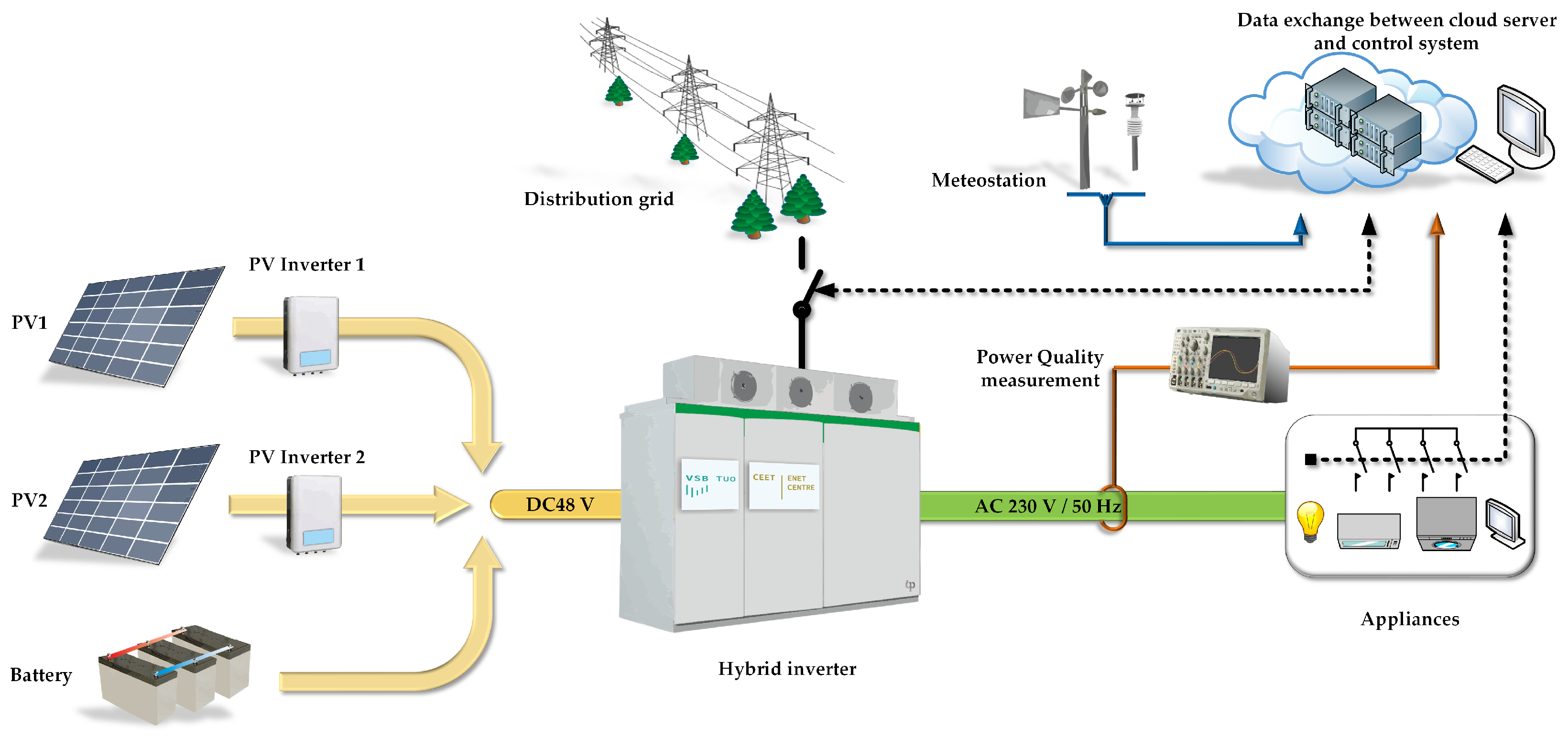
The microgrid household platform (MHP) serves as a testbed for simulating the electricity consumption of a house in Central Europe. At its core, the system can be characterized as a small-scale microgrid system, as illustrated in Figure 1. During non-winter periods, the MHP operates in off-grid mode as the default configuration, while distribution grid interconnection is employed only as a backup measure in the event of an energy shortage. The MHP is an off-grid system with a hybrid AC-DC architecture. The fundamental part of the MHP is a hybrid XW+ 8548 inverterwith a rated power of 6.8 kW. The MHP is structured in two principal sections. The first is organized around a primary 48 V DC bus, whereas the second section is based on a 230 V AC bus [14,46].

The DC section of the MHP comprises two Conext 80 600 PV inverters, which convert the electricity generated by two photovoltaic (PV) strings. The first PV string is based on monocrystalline PV arrays, while the second PV string consists of polycrystalline arrays, each with a rated power of 2 kW. The first photovoltaic string is on a movable structure that tracks the Sun’s position in the sky. This is known as a photovoltaic tracker. The second photovoltaic string is located on the roof of the MHP building, where the technical facilities of the microgrid and the research laboratory are located. The storage system consists of Hawker 12XFC115 batteries with a nominal voltage of 12 V and a nominal capacity of 115 Ah. The batteries are assembled in a battery box, forming four groups of four cells. Consequently, the DC bus voltage ranges between 44 and 56 V, depending on the state of the battery charge and the charging process [14,46].

The AC section of the MHP is based on a 230 V bus operating at a frequency of 50 Hz. This bus is directly connected to the hybrid inverter, which supplies individual household appliances. Power Quality (PQ) measurements were carried out in accordance with the European standards summarized in

Table 1. European standards: limit values for PQPs [7,47].

European Power Quality Standards
Standard	Limit Values
EN 50160 [7]	Voltage frequency: Mean value over 10 s: ±1% (49.5–50.5 Hz) for 99.5% of a week. Allowed range: −6%/+4% (47–52 Hz) for 100% of a week. Voltage magnitude variations: 10 min RMS values: ±10% for 95% of a week. Harmonic voltage (% of fundamental supply voltage): 3rd: 5%; 5th: 6%; 7th: 5%; 9th: 1.5%; 11th: 3.5%; 13th: 3%; 15th: 0.5%; 17th: 2%; 19th: 1.5%; 23rd and 25th: –
EN 61000-2-2 [47]	Voltage frequency: ±2% Voltage magnitude variations: ±10% (applied for 15 min). Harmonic voltage: 5th: 6%; 7th: 5%; 11th: 3.5%; 13th: 3 Total Harmonic Distortion (THD): 8%

. For this purpose, a KMB SMC 144 PQ analyzer was used. This device monitors PQ across the AC bus and is specifically designed to monitor energy consumption and power quality remotely. The recorded data is stored on a cloud server, which also allows it to be used for subsequent optimization processes. Furthermore,

Table 2. The parameters of the home appliances used in the research [14,46].

Appliance	$\mathit{PL}$ (kW)			$\mathit{PF}$ (-)		$\mathit{THD}$ (%)
	Avg	Min	Max	Avg	Character	${\mathit{THD}}_{\mathit{u}}$	${\mathit{THD}}_{\mathit{i}}$
No appliance	-	-	-	-	-	2.1	42.1
Kettle	619.10	617.02	628.32	1.0	R	4.2	6.2
Fridge	207.56	195.45	219.51	0.7	L	2.7	11.6
AC—Air Conditioning	880.00	852.45	910.03	0.9	L	2.1	10.2
Microwave	203.01	76.81	1348.01	0.8	L	5.1	56.8
TV—Television	44.01	42.82	50.51	0.6	C	3.0	20.9
Lights (LED Lights)	156.00	152.51	165.12	0.8	C	2.8	77.6

presents a selection of the electrical characteristics of the appliances used in the experimental setup [14,46].

In this study, we used meteorological data comprising measurements conducted by a certified meteorological station operated of the Czech Hydrometeorological Institute (CHMI). The meteorological station is situated at the precise location of the MHP facility, within the VSB Technical University of Ostrava campus. Similarly to PQP data, meteorological records are stored in a cloud-based database to facilitate subsequent research and analysis [14].

3. Mathematical Description

3.1. K-Nearest Neighbors (KNN) Algorithm

The K-Nearest Neighbors (KNN) algorithm is a machine learning technique that can be used for classification and regression purposes [48,49]. The basic idea of KNN regression is to compute the mathematical average of the numerical target of the k nearest neighbors’ output. For example, if $k=2$, two samples with the minimum distance value were selected from the tested sample. The regression output for this tested sample will be the average of the target output for these two samples, with similar results when the assigned value of k is larger than 2. In these experiments, the Euclidean distance was used to measure the distance between the samples, as in (1) [50], and the KNN algorithm was applied for different numbers of k (e.g., $k=5, k=10, k=15$). The best results were obtained when using $k=5$ and $k=10$.

$$d(a,b)=\sqrt{\sum _{i=1}^n{(a_i-b_i)}^2}.$$

(1)

where $a_i$ and $b_i$ are data points, i is the number of the subsequent sample, and n is the size of the data sample.

3.2. Decision Tree (DT)

Decision Trees (DTs) are machine learning methods used for classification (CT) or regression (RT) [51,52]. The goal is to create a model to predict a class target output or a numerical value as a classification or regression tree (RT), respectively. The basic idea for a regression tree is to divide a dataset into smaller subgroups based on features of the dataset, then fit a simple regression model for each group. Ensemble decision trees were used in this study to forecast PQPs to improve forecast accuracy. An ensemble decision tree merges many sub-decision trees to improve the forecasting performance of each regression tree alone. There are two main types of ensemble models: bagging and boosting decision trees [53].

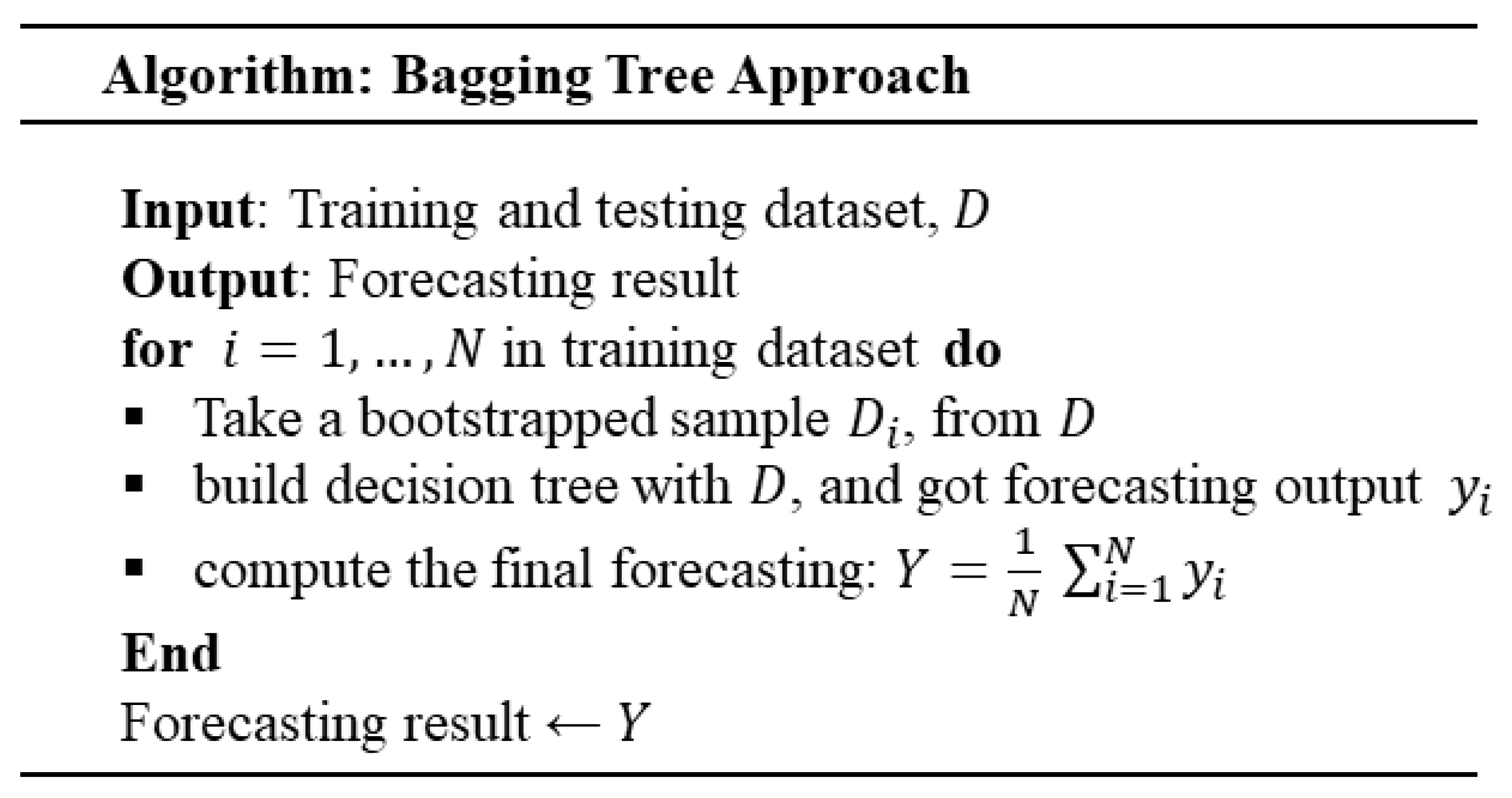
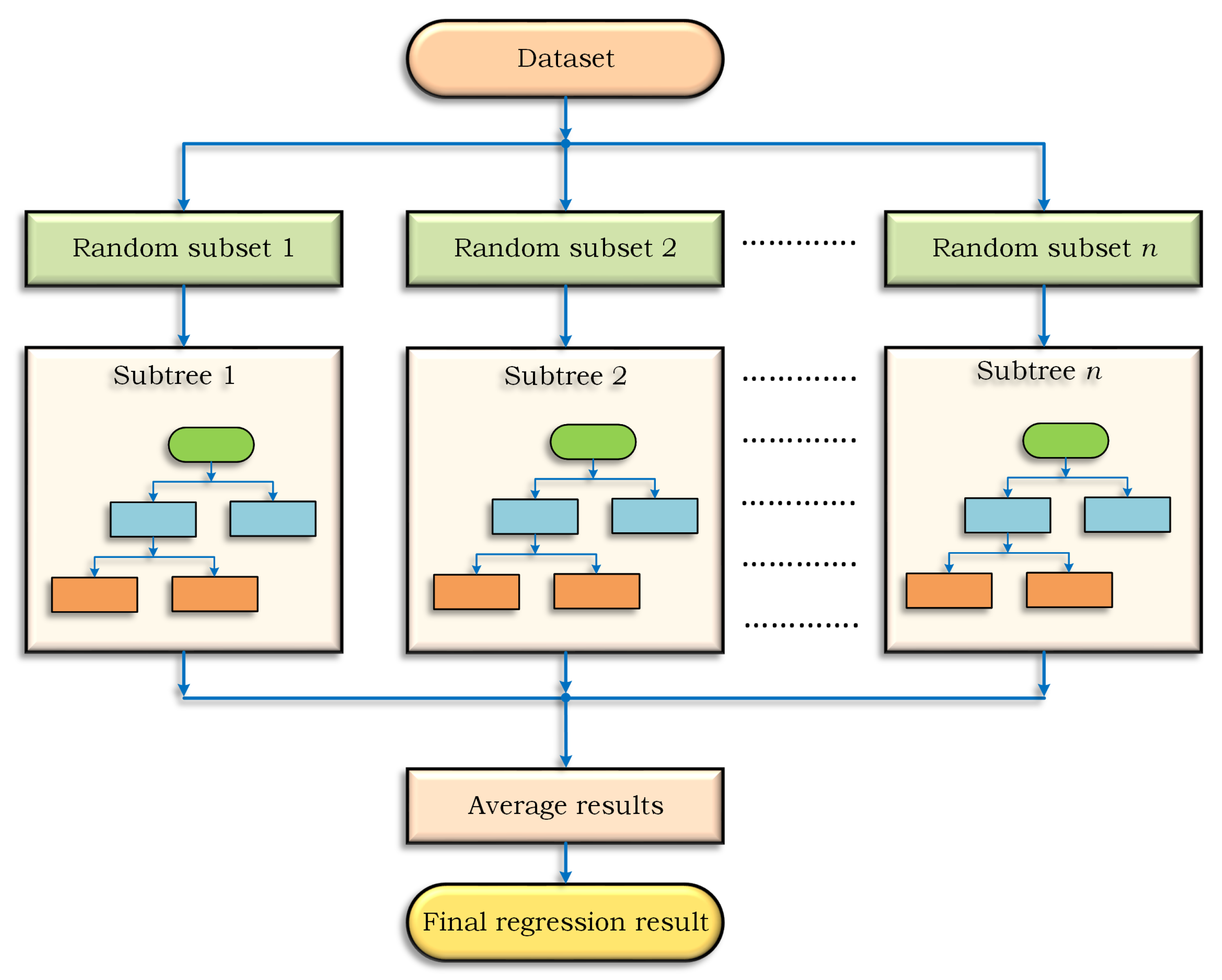
A bagging decision tree is used for the training of a number of individual trees in parallel. Each tree is trained by selecting a random subset of the main dataset. After dividing the main dataset randomly into sub-datasets, each sub-dataset is used to train sub-regression trees in parallel. Since all datasets are passed to all subtrees, the final regression result of the bagging tree will be the average of the outputs of these subtrees, as can be seen in Figure 2 [54].

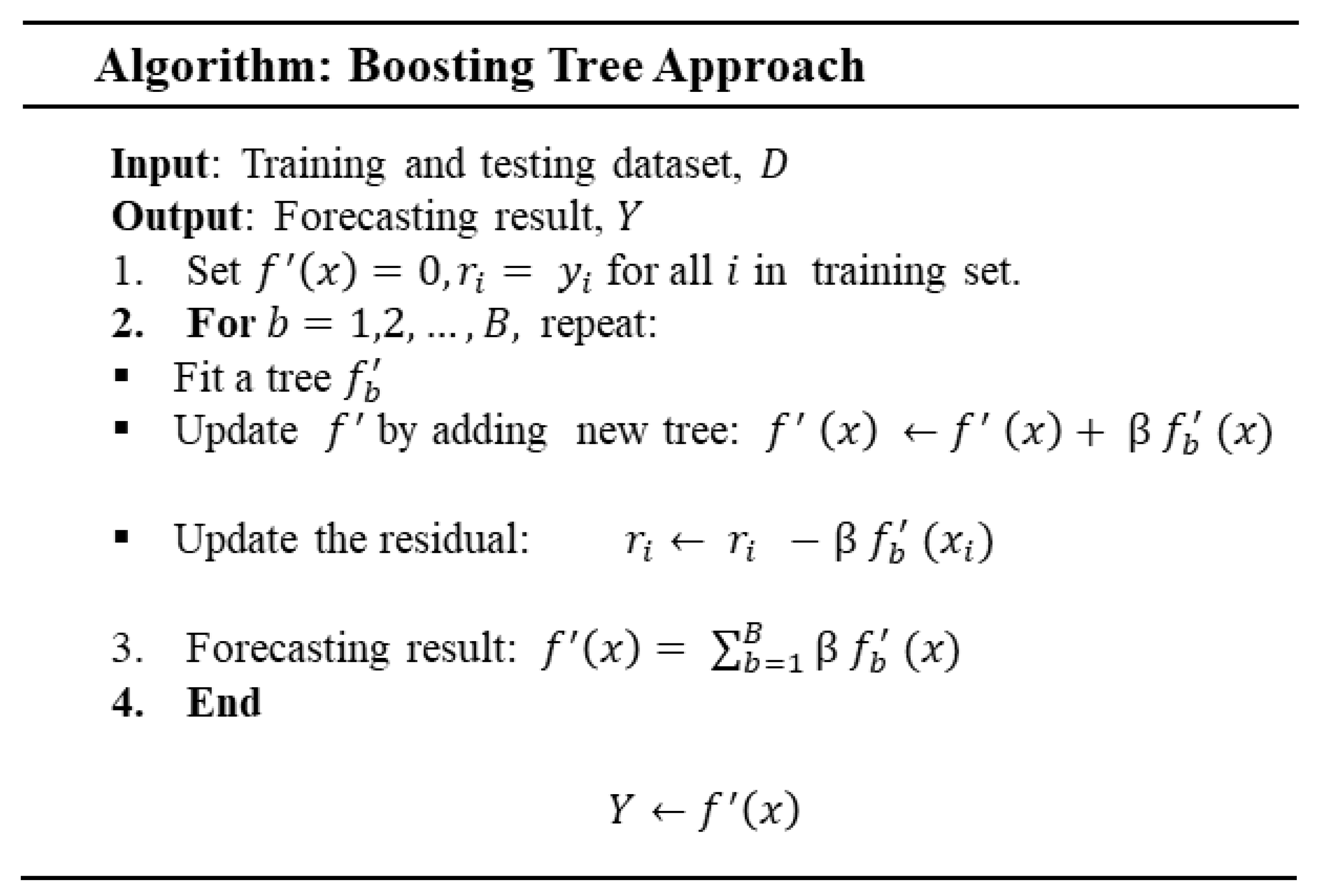
A boosting decision tree sequentially trains several individual trees. Each individual tree learns from the mistakes of the previous tree, as in (2) and Figure 3 [54].

$$Y=y_1+(e_1\times \beta )+(e_2\times \beta )+\cdots +(e_n\times \beta ).$$

(2)

where Y is the final output of the model, $y_1$ is the output of the first tree, $e_1$ is the residual error of the first tree, and $\beta$ is the learning rate.

Figure 4, Figure 5 and Figure 6 show the algorithmic steps and pseudocode for KNN, BGDT, and BODT, respectively.

4. Proposed Model

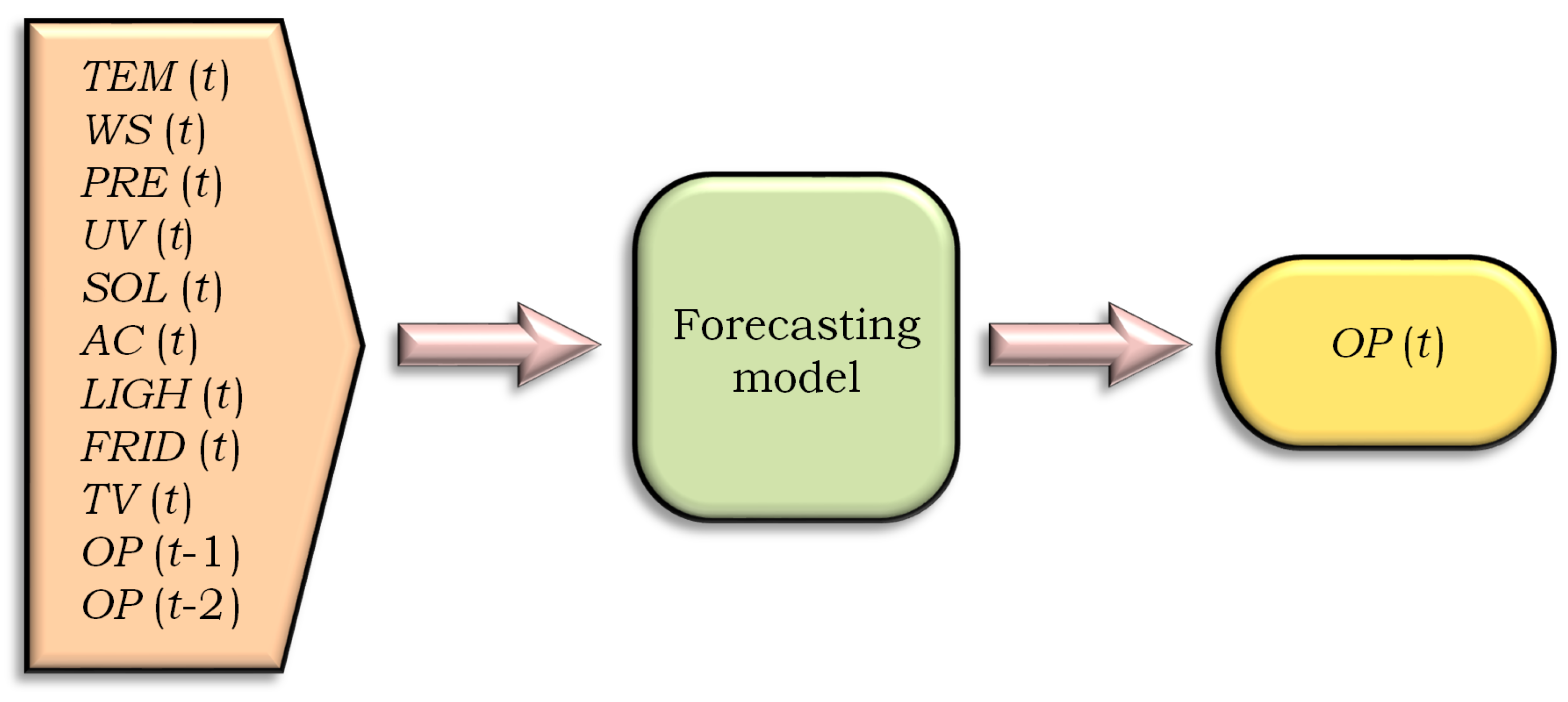
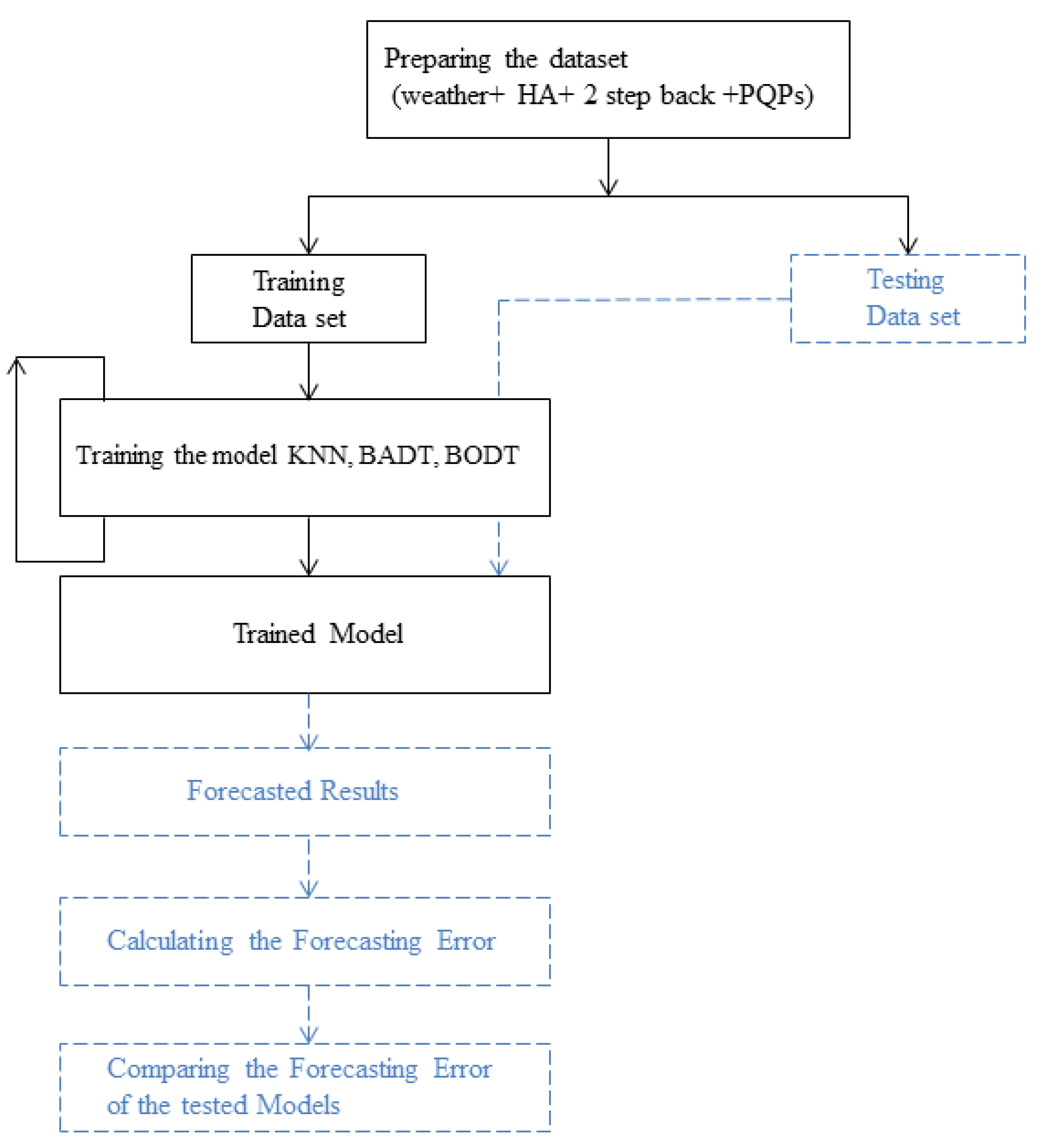
Based on the results achieved in our last study [14] that tested seven models for PQP forecasting, we concluded that the ensemble decision tree achieved better results than other compared models. Therefore, in this work, the ensemble tree was chosen as a comparison forecasting model to predict the $TH{D}_u$, $TH{D}_i$, $PL$, $PF$, and U parameters. The selected input variables are global solar irradiance, air temperature, wind speed, air pressure, UV, home appliances, and one and two back steps of each target output. The output PQPs are U, $TH{D}_u$, $TH{D}_i$, ($PF$), and ($PL$), as can be seen in the experimental scheme in Figure 7 and the training and testing procedure in Figure 8.

The Root Mean Square Error (RMSE) [55] was used to analyze and compare the forecast results, as in (3).

$$RMSE=\sqrt{{\displaystyle \frac{1}{n}}\sum _{j=1}^n{\left(M_j-P_j\right)}^2}.$$

(3)

where $M_j$ is the measured value, $P_j$ is the output of the model, and n is the number of data samples.

Forecasting models were designed and results were compared using MATLAB in the following steps:

• Reading, uploading the dataset, and selecting input variables;
• Adding the first and second back steps for each target output into the input variables;
• Dividing the dataset into training and testing datasets;
• Training and testing forecasting models (BADT, BODT, KNN (k= 5), and KNN (k = 10)) with each model setup for prediction of five PQPs;
• Calculating the forecasting errors, correlation coefficient, and execution time;
• Plotting the results of the designed models.

The experiments were conducted on a laptop with the following hardware specifications: Intel(R) Pentium(R) 5405U CPU @ 2.30 GHz and 4.00 GB of installed RAM (3.88 GB usable). The software environment consisted of the Windows 11 Home operating system, version 21H2, and MATLAB R2018a as the programming language platform. Although the hardware can be considered relatively outdated by current standards, the experimental procedures did not require substantial computational resources. Hence, the available configuration was sufficient to reliably perform all simulations and data analyses.

4.1. Dataset

The dataset used in this experiment is provided by the off-grid system installed at the ENET Centre, as can be seen in Figure 1, and the dataset is available for free download online [56]. The dataset consists of weather conditions (such as air temperature, wind speed, air pressure, ultraviolet radiation, etc.); the U, $TH{D}_u$, $TH{D}_i$, $PF$, and $PL$ parameters; and consumed loads for four types of home appliances (AC/heating, lights, fridge, and TV).

4.2. Experimental Description

The experiments tested the following models to forecast the mentioned PQPs: BGDT, BODT, and KNN (with $k=5$ and $k=10$). The power parameters are U, $TH{D}_u$, $TH{D}_i$, $PL$, and $PF$. The designed models were created using the following input variables: air temperature ($TE$), wind speed ($WS$), air pressure ($PRE$), ultraviolet radiation ($UV$), solar irradiance ($SOL$), power consumed by home appliances (AC/heating, lights, fridge, and TV), and two steps of each power quality parameter.

For example, in the voltage forecasting model at time t, we utilized the following variables: $T{E}_t$, $W{S}_t$, $PR{E}_t$, $U{V}_t$, $SO{L}_t$, $AC\_heatin{g}_t$, $Light{s}_t$, $Fridg{e}_t$, $T{V}_t$, $U_{t-1}$, and $U_{t-2}$. The measured voltage ($U_t$) at the same time step was used as the target output, applying the same procedure for the rest of the forecasting models. The $KNN$ algorithm was applied for different numbers of k. The best results were obtained when setting k to 5 and 10; therefore, $KNN$ models with $k=5$ and $k=10$ were selected for comparison in this study.

5. Results

5.1. Forecasting Results

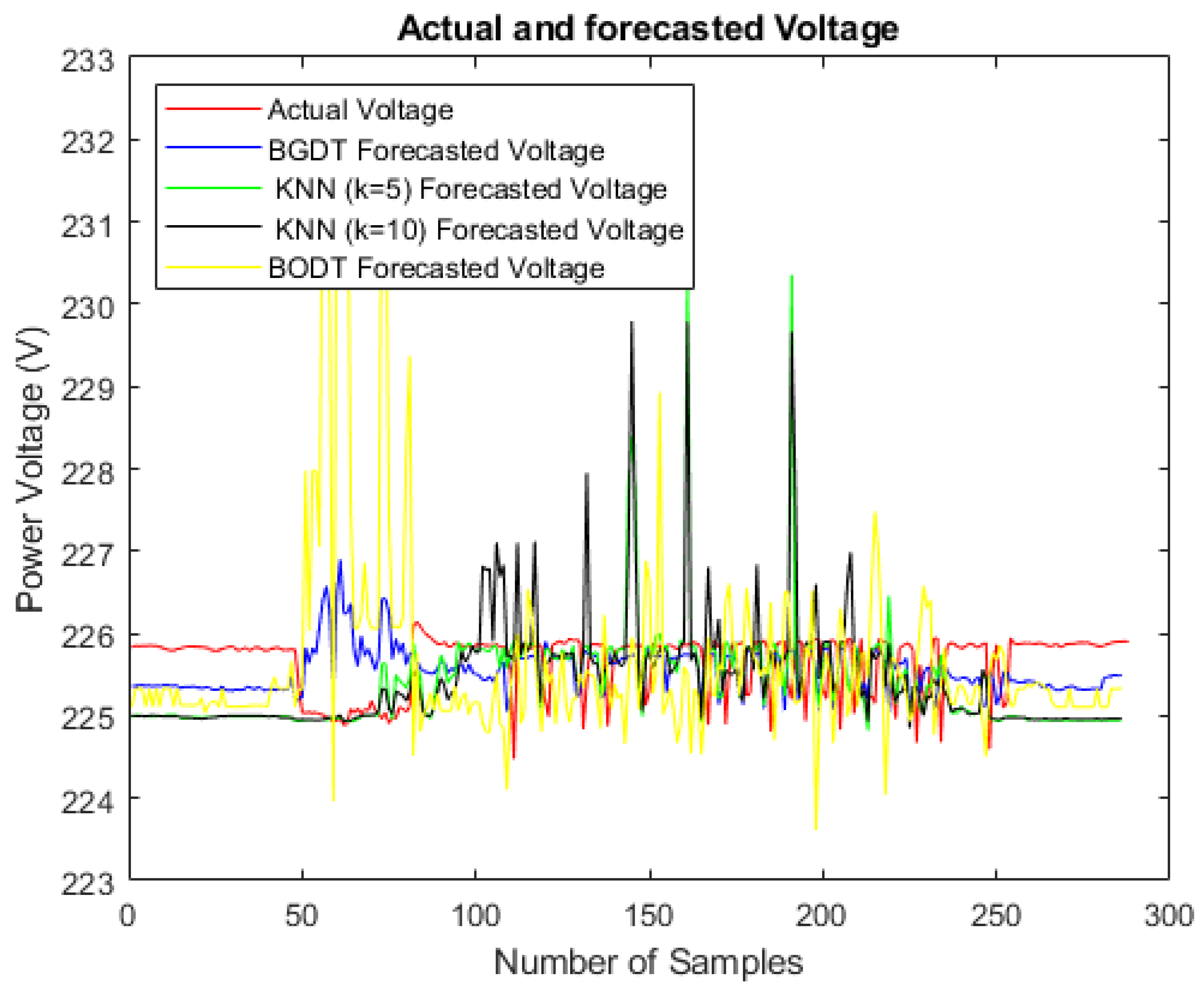
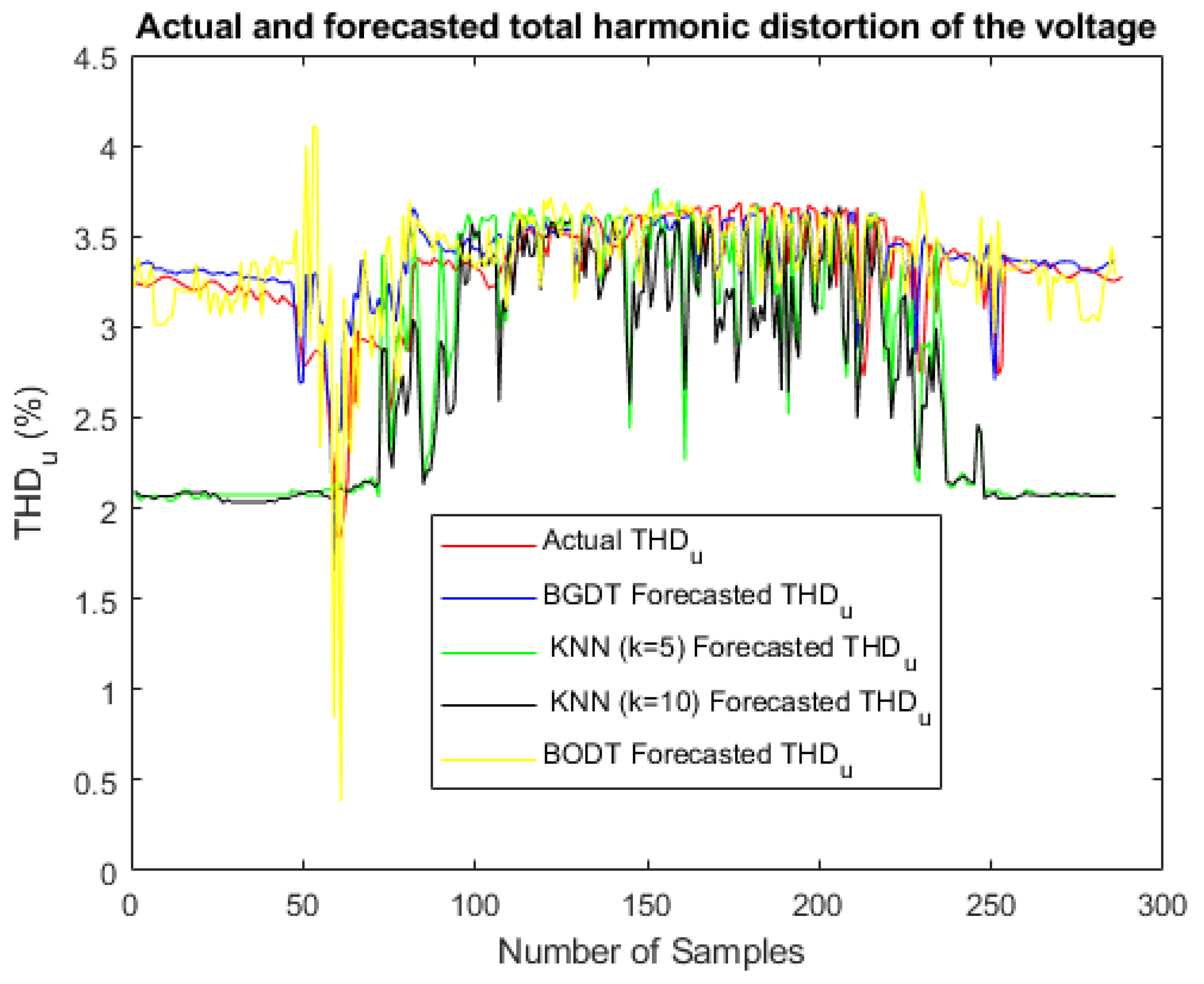
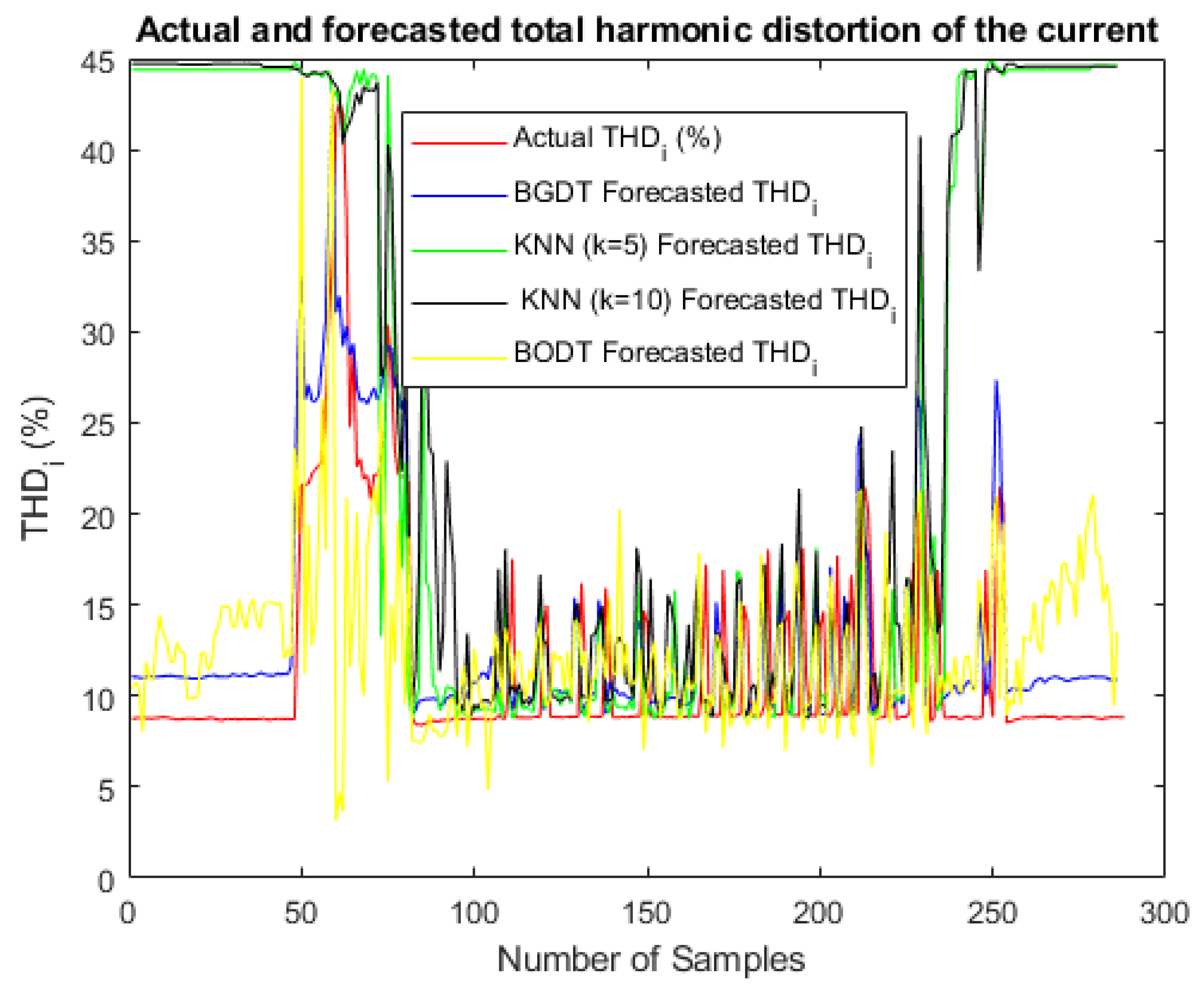
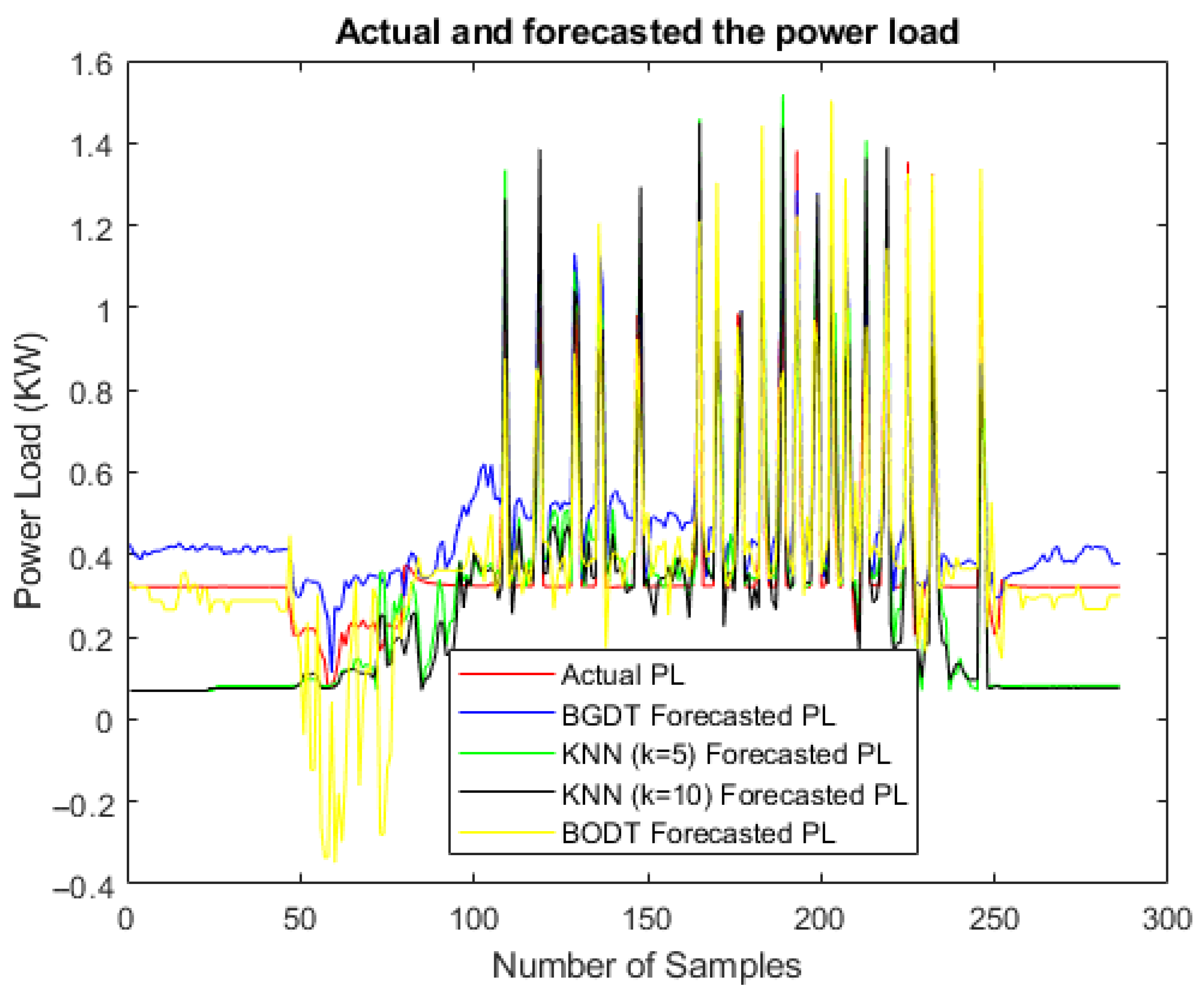
The Pearson correlation coefficient and Root Mean Square Error (RMSE) were calculated for each model.

Table 3. Root Mean Square Error (RMSE) of forecasts obtained by BGDT for the period of 29 June–8 July 2019.

Date	U (V)	${\mathit{THD}}_{\mathit{u}}$ (%)	${\mathit{THD}}_{\mathit{i}}$ (%)	$\mathit{PF}$ (-)	$\mathit{PL}$ (kW)
2019-06-29	0.193	0.004	0.075	0.002	0.012
2019-06-30	6.406	0.085	0.317	0.009	0.006
2019-07-01	18.69	0.199	0.067	0.053	0.027
2019-07-02	0.019	0.005	0.602	0.003	0.017
2019-07-03	0.077	0.019	1.503	0.006	0.026
2019-07-04	0.096	0.016	1.389	0.001	0.021
2019-07-05	0.052	0.068	1.165	0.012	0.081
2019-07-06	0.053	0.059	0.840	0.012	0.034
2019-07-07	0.077	0.106	0.201	0.007	0.067
2019-07-08	0.081	0.082	1.777	0.005	0.095

,

Table 4. Root Mean Square Error (RMSE) of forecasts obtained by BODT for the period of 29 June–8 July 2019.

Date	U (V)	${\mathit{THD}}_{\mathit{u}}$ (%)	${\mathit{THD}}_{\mathit{i}}$ (%)	$\mathit{PF}$ (-)	$\mathit{PL}$ (kW)
2019-06-29	0.554	0.015	1.205	0.005	0.008
2019-06-30	39.04	0.167	0.353	0.002	0.001
2019-07-01	133.0	0.549	1.461	0.122	0.032
2019-07-02	0.237	0.028	1.579	0.004	0.012
2019-07-03	0.404	0.036	3.259	0.009	0.066
2019-07-04	0.503	0.046	0.353	0.009	0.012
2019-07-05	0.586	0.015	0.898	0.016	0.004
2019-07-06	0.449	0.099	0.236	0.016	0.018
2019-07-07	0.711	0.084	2.031	0.007	0.009
2019-07-08	0.021	0.043	0.918	0.013	0.011

,

Table 5. Root Mean Square Error (RMSE) of forecasts obtained by KNN ($k=5$) for the period of 29 June–8 July 2019.

Date	U (V)	${\mathit{THD}}_{\mathit{u}}$ (%)	${\mathit{THD}}_{\mathit{i}}$ (%)	$\mathit{PF}$ (-)	$\mathit{PL}$ (kW)
2019-06-29	0.030	0.031	0.455	0.015	0.012
2019-06-30	0.911	0.026	0.538	0.015	0.013
2019-07-01	0.060	0.105	1.249	0.033	0.066
2019-07-02	0.902	0.020	1.226	0.001	0.011
2019-07-03	0.653	0.062	2.009	0.006	0.023
2019-07-04	1.261	0.126	6.713	0.010	0.040
2019-07-05	0.127	0.445	11.59	0.012	0.069
2019-07-06	0.178	0.530	12.58	0.008	0.102
2019-07-07	0.105	0.440	9.860	0.001	0.049
2019-07-08	0.260	0.531	13.87	0.008	0.080

and

Table 6. Root Mean Square Error (RMSE) of forecasts obtained by KNN ($k=10$) for the period of 29 June–8 July 2019.

Date	U (V)	${\mathit{THD}}_{\mathit{u}}$ (%)	${\mathit{THD}}_{\mathit{i}}$ (%)	$\mathit{PF}$ (-)	$\mathit{PL}$ (kW)
2019-06-29	0.049	0.063	0.582	0.017	0.007
2019-06-30	0.143	0.062	0.540	0.009	0.017
2019-07-01	0.038	0.130	1.248	0.042	0.073
2019-07-02	0.874	0.033	1.614	0.001	0.002
2019-07-03	0.691	0.001	2.469	0.005	0.013
2019-07-04	1.245	0.179	7.274	0.011	0.050
2019-07-05	0.101	0.507	12.59	0.009	0.081
2019-07-06	0.148	0.589	13.62	0.006	0.116
2019-07-07	0.079	0.524	10.83	0.002	0.066
2019-07-08	0.225	0.622	15.04	0.005	0.098

show the RMSE error achieved by the BGDT, BODT, KNN ($k=5$), and KNN ($k=10$) algorithms, respectively, for the ten tested days from 29 June to 8 July 2019.

Table 7. RMSE Comparison of tested models.

Model	U (V)	${\mathit{THD}}_{\mathit{u}}$ (%)	${\mathit{THD}}_{\mathit{i}}$ (%)	$\mathit{PF}$ (-)	$\mathit{PL}$ (kW)
BGDT	2.566	0.056	0.616	0.011	0.039
BODT	17.540	0.109	1.226	0.020	0.028
KNN (k = 5)	0.367	0.230	6.011	0.011	0.046
KNN (k = 10)	0.359	0.271	6.581	0.011	0.052

shows the average error achieved by all tested models, which explains the comparison results of the performance of the investigated forecasting systems. Figure 9, Figure 10, Figure 11, Figure 12 and Figure 13 show the measured and forecast values of the U, $TH{D}_u$, $TH{D}_i$, $PF$, and $PL$, respectively.

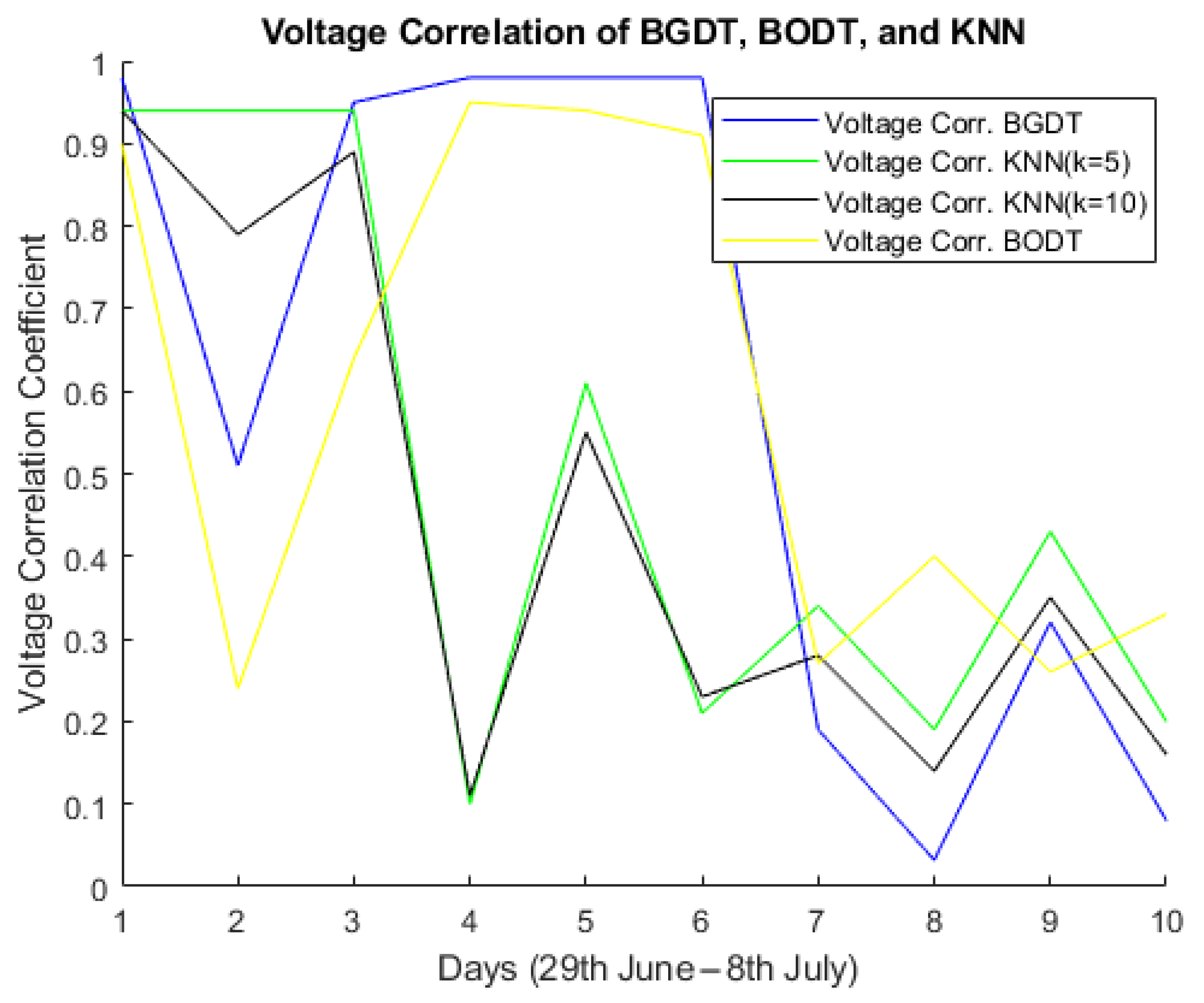
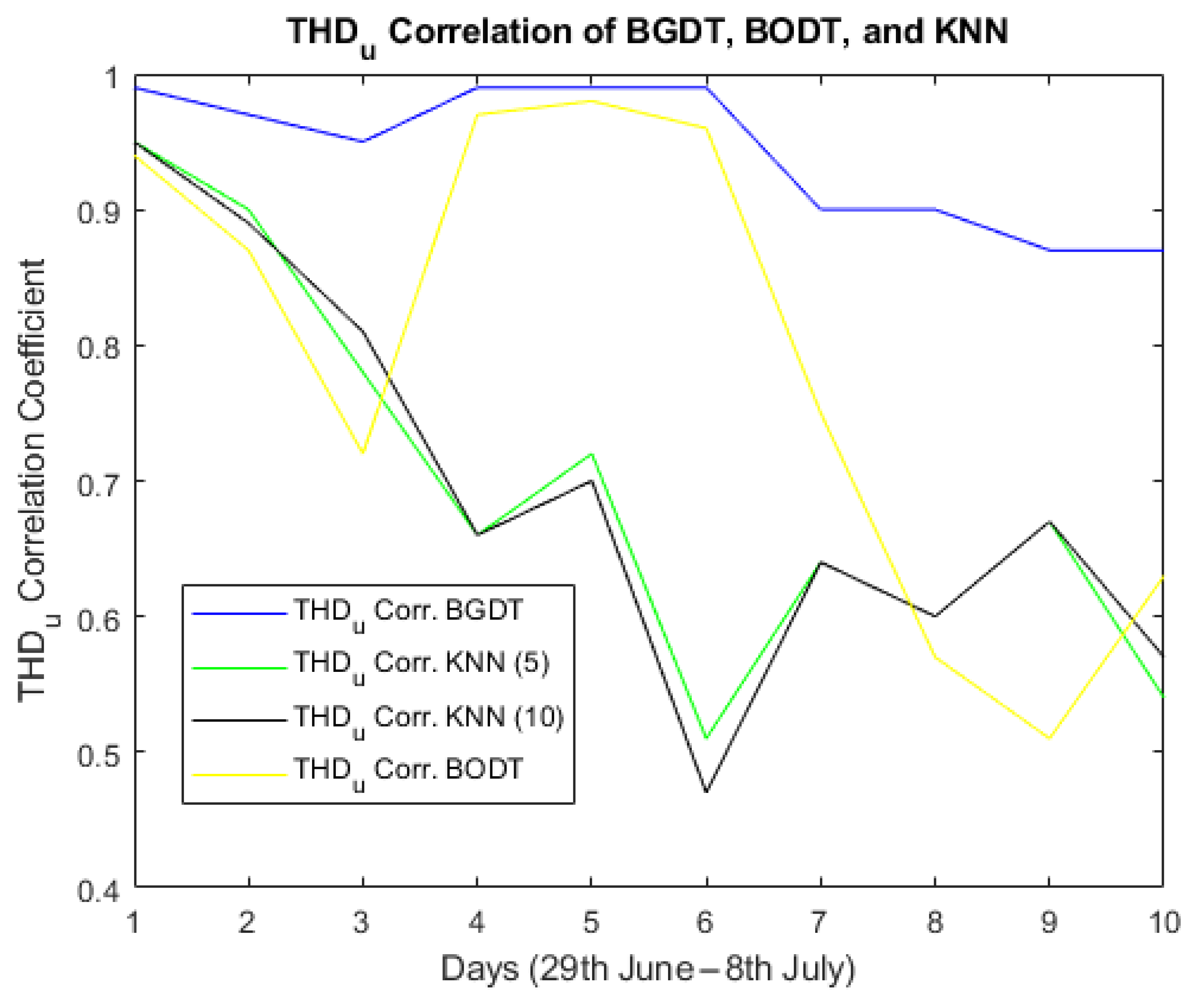
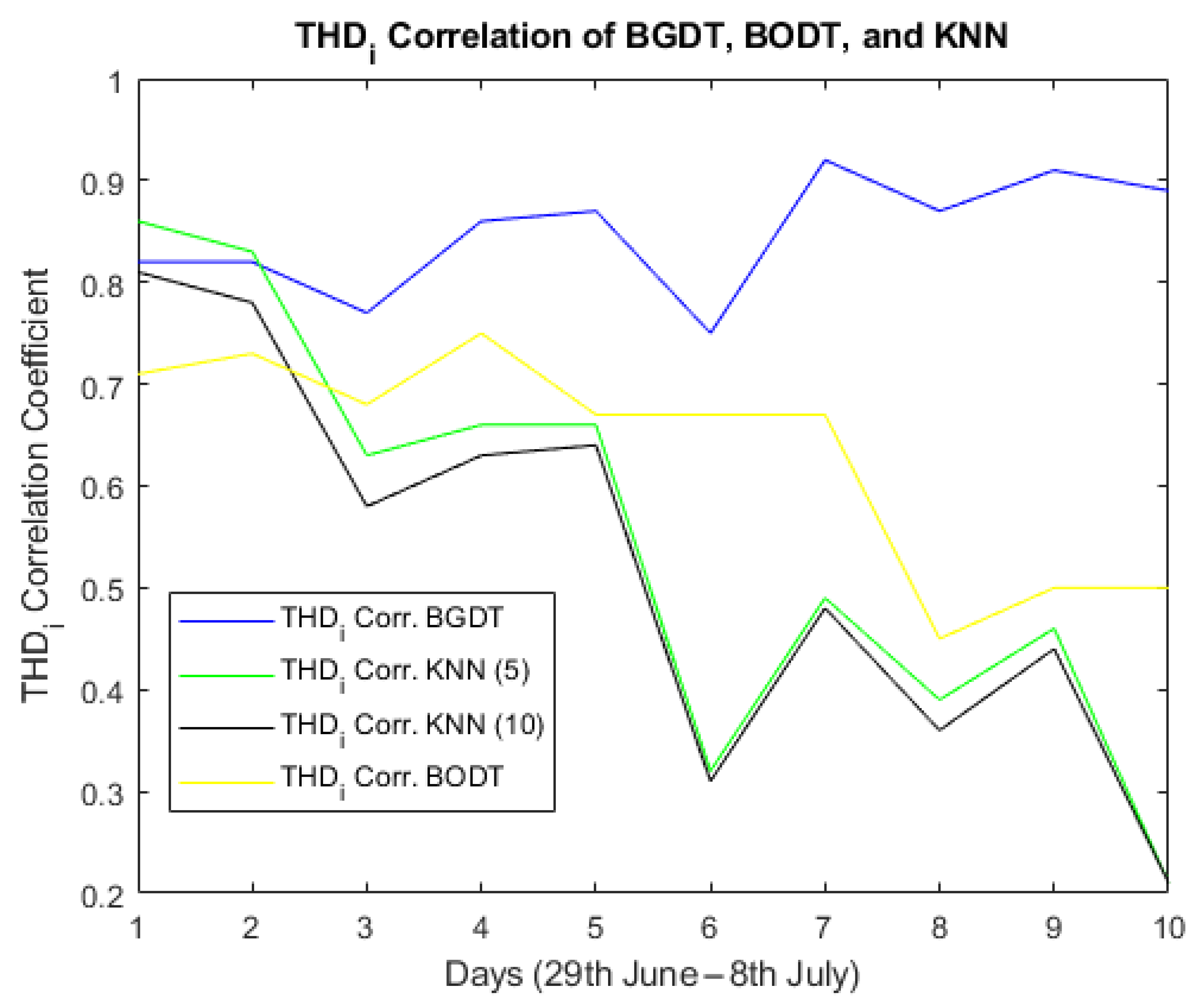
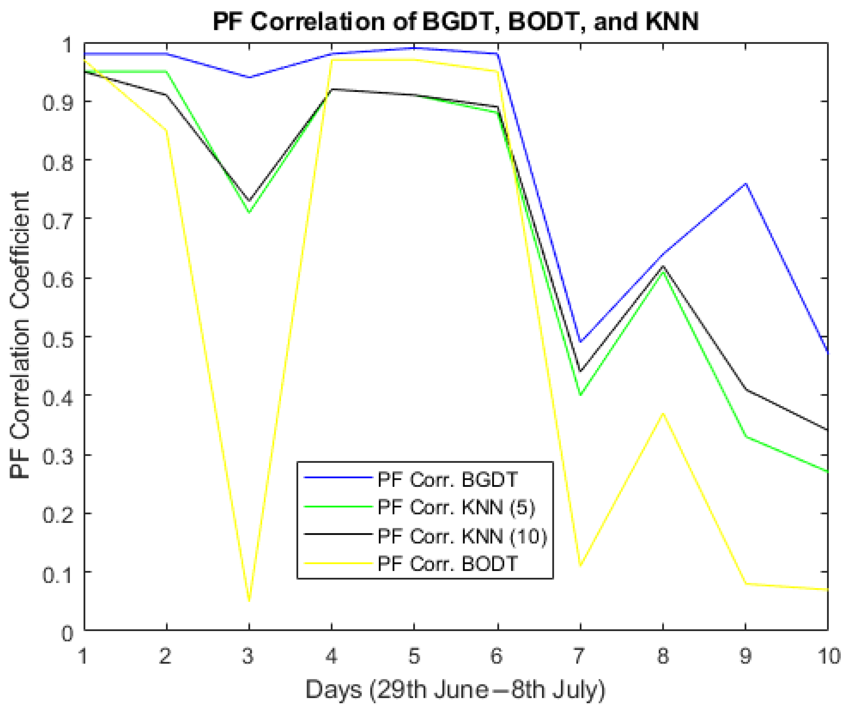
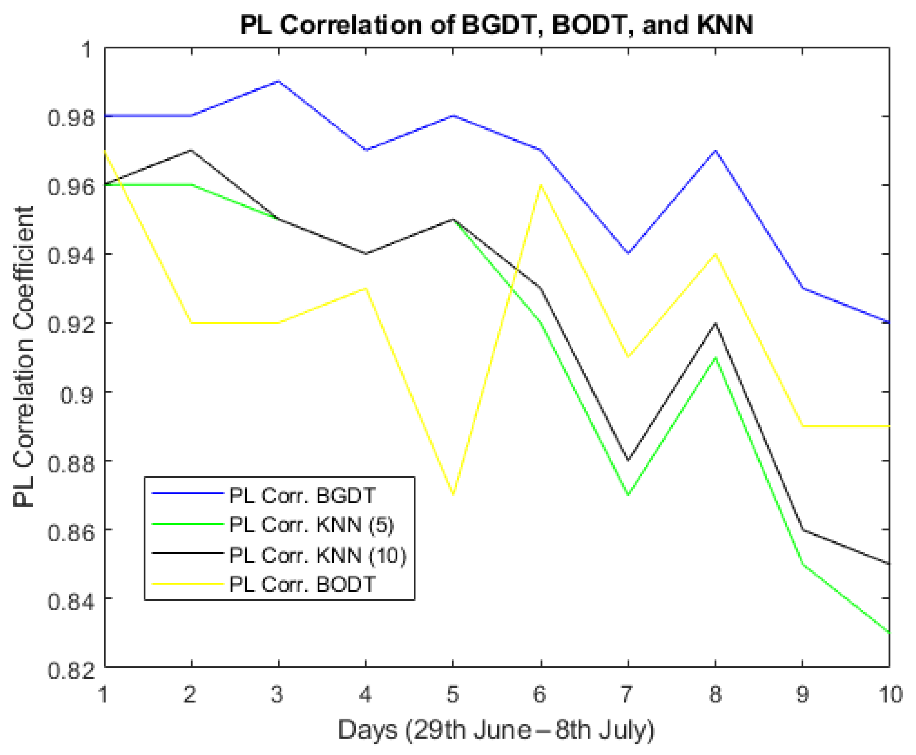
In Figure 14, Figure 15, Figure 16, Figure 17 and Figure 18 show the correlation coefficients between the actual and forecasted values of the U, $TH{D}_u$, $TH{D}_i$, $PF$, and $PL$ parameters.

5.2. Execution Time Results

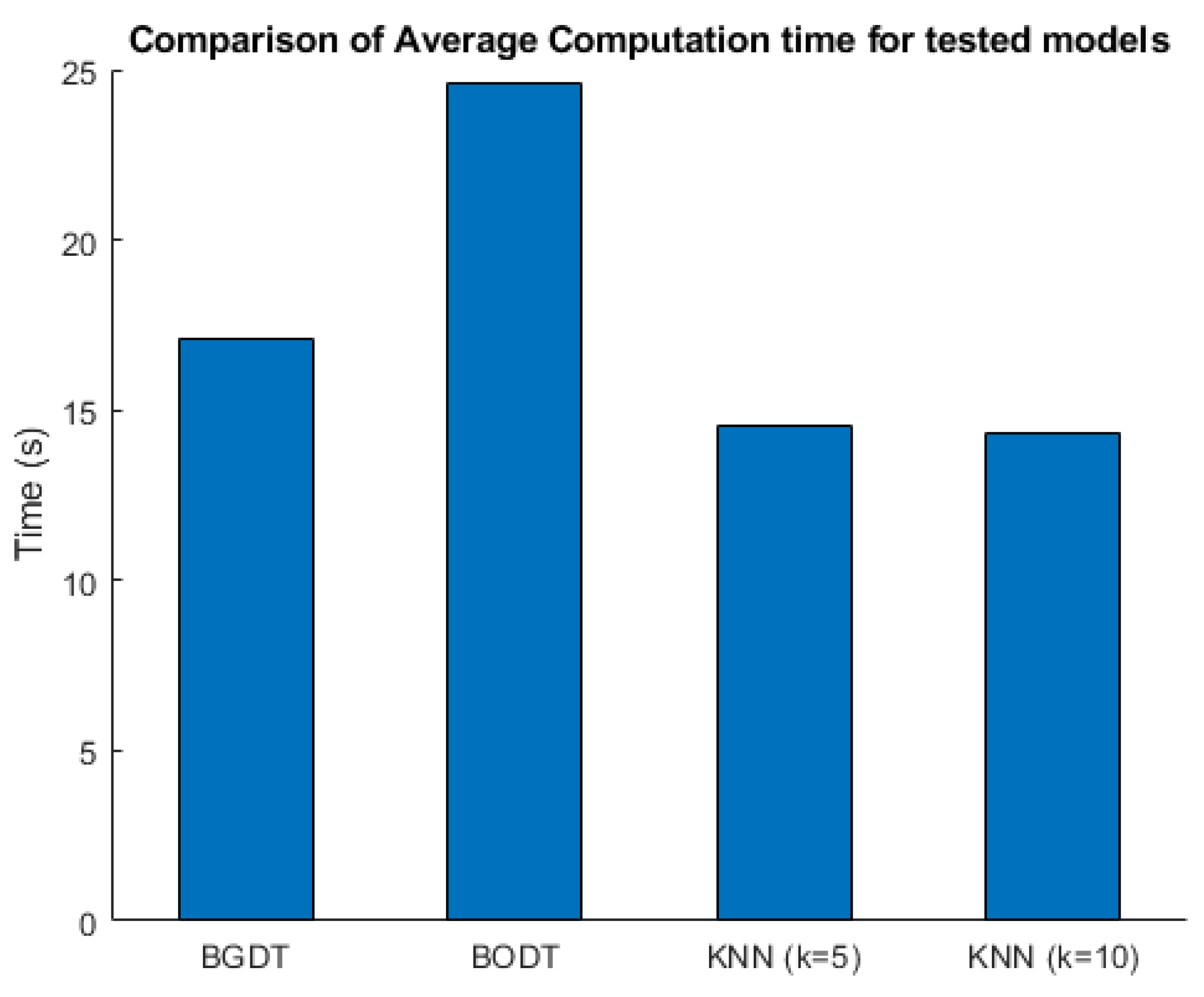
The computation time for forecasting all parameters was computed, as can be seen in

Table 8. Computation time of the tested models to forecast all the tested PQPs in seconds.

Date	BGDT (s)	BODT (s)	KNN (k = 5) (s)	KNN (k = 10) (s)
2019-06-29	16.92	25.34	14.61	14.57
2019-06-30	16.95	25.24	14.85	14.35
2019-07-01	17.07	22.99	14.52	14.46
2019-07-02	17.01	24.39	14.58	14.55
2019-07-03	17.06	24.50	14.30	14.48
2019-07-04	17.06	24.15	14.76	14.08
2019-07-05	17.29	24.83	14.39	14.22
2019-07-06	17.20	24.42	14.36	14.22
2019-07-07	17.13	24.96	14.36	14.29
2019-07-08	17.50	24.91	14.36	14.24
Average	17.12	24.57	14.51	14.35

, which depicts an average execution time of 10 days for the tested models. Figure 19 shows a comparison of the computation time for learning and testing of the proposed methods.

6. Discussion

This section compares the forecasting results and computation times of the proposed models. The objective is to find the best forecasting model for each parameter. Based on the experimental results presented in Table 3, Table 4, Table 5 and Table 6, we present the REMS error for the tested models and correlation results between the measured values and output of forecasting models, as shown in Figure 14, Figure 15, Figure 16, Figure 17 and Figure 18.

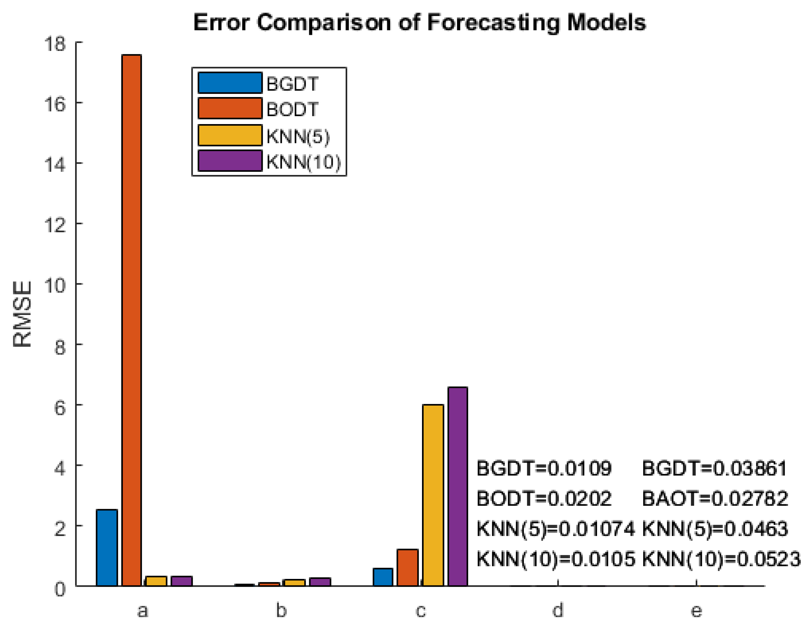
• U: The average values of the forecasting error for 10 days for four designed models ranged between 0.359 and 17.54 V; the lowest value was obtained by KNN ($k=10$), followed by KNN ($k=5$) and BGDT, with the worst performance achieved by BODT.
• $TH{D}_u$: The average RMSE values for the 10 tested days between the actual and forecasted $TH{D}_u$ values were 0.05612, 0.1085, 0.229, and 0.270 for the BGDT, the BODT, KNN ($k=5$), and KNN ($k=10$) algorithms, respectively.
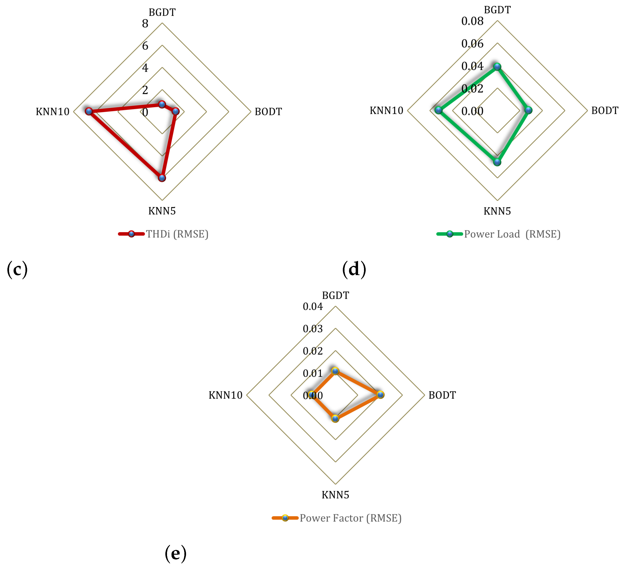
• $TH{D}_i$: The lowest average error between the measured and predicted values of $TH{D}_i$ for the 10 tested days was about 0.616, obtained by BGDT, followed by BODT, which obtained an error close to 1.226, while the worst results of close to 6.00 and 6.58 were obtained by KNN ($k=5$) and KNN ($k=10$), respectively.
• $PF$: The best average error value over the 10 tested days for $PF$ forecasting was 0.01. The best results were obtained by KNN ($k=10$), followed by KNN ($k=5$) and BGDT. BODT obtained the worst error among the tested models—close to 0.02.
• $PL$: The lowest average error for $PL$ forecasting was close to 0.0278, and obtained by BODT, followed by BGDT, with an error close to 0.038, and KNN ($k=5$), with an error of 0.046. KNN ($k=10$) obtained the largest error, with a value of around 0.052.

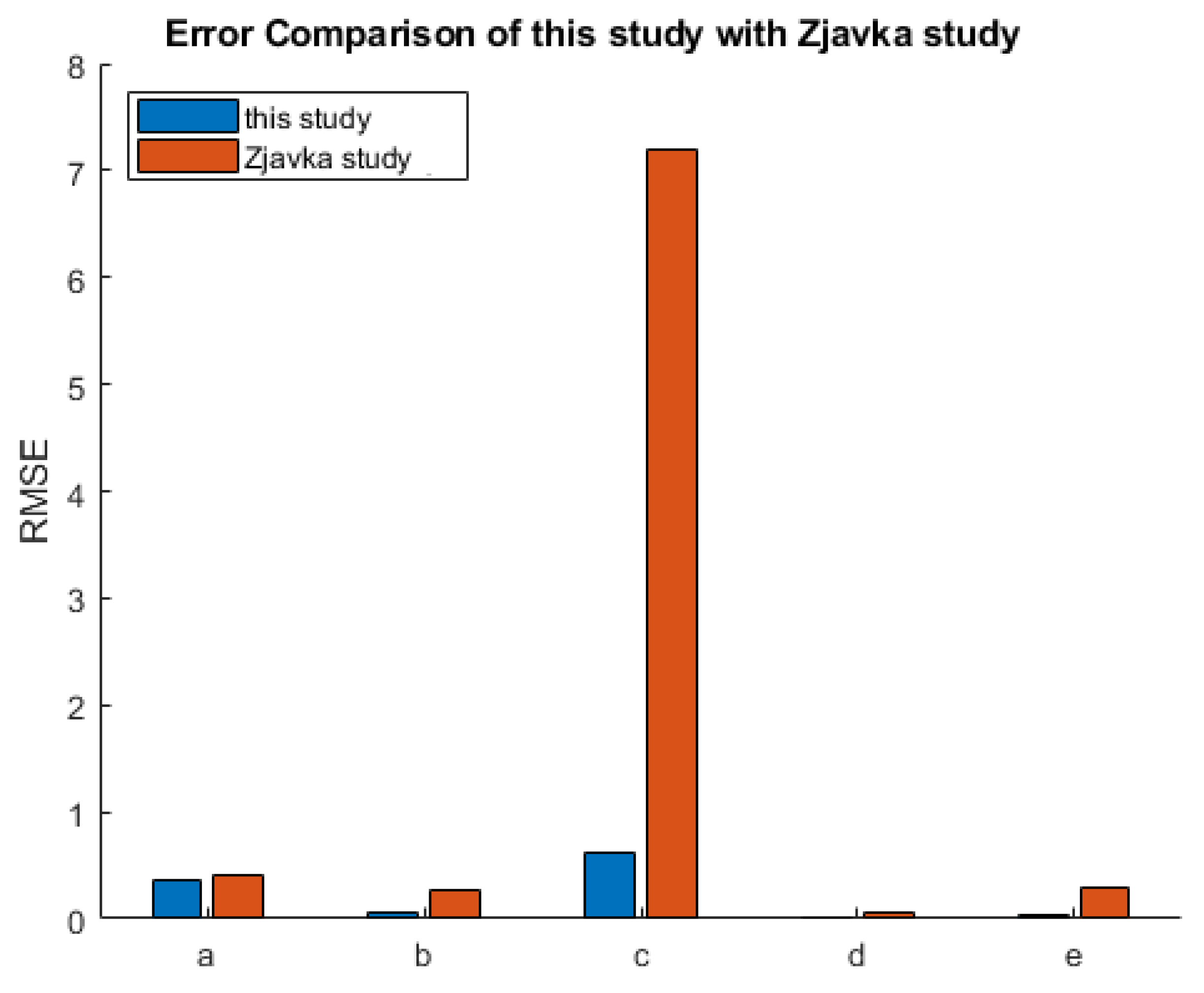
Figure 20 shows a comparison of the forecasting errors. The results reported in this study show a slight improvement compared with the experiments reported in [8], as can be seen in Figure 21. Figure 22 shows a radar graph that represents a comparison of performance models. Figure 22a–e show the RMSE of the forecast models for U, $TH{D}_u$, $TH{D}_i$, $PL$, and $PF$, respectively.

In order to better illustrate the valuable proportion of the obtained results, Figure 23 presents a comparison of RMSE values for all parameters in one bar chart.

Computation time: The computation time required to execute forecasting of all tested parameters was calculated. The KNN algorithm took the shortest execution time, lasting approximately 14 s, while the decision tree took 17 s and BGDT and BODT too 24 s.

In comparison with the results obtained in [8], the value of RMSE can be presented as follows:

• The minimum RMSE value for U was about 0.40, and it was obtained by the bagging DT algorithm.
• The smallest error value of $TH{D}_u$ was close to 0.258, and it was obtained by the bagging DT algorithm.
• The smallest error value of $TH{D}_i$ was 7.19, obtained when using D-PNN.
• The minimum error value of about 0.0467 for the power factor ($PF$) was obtained using D-PNN.
• For the power load ($PL$), the smallest error value of 0.290 was obtained when using DLT.

In our experiments, in addition to the weather conditions, two back steps of each parameter output and home appliances were used as input variables. Using home appliances as input variables is a crucial consideration when designing a smart control system. Smart scheduling of home appliances resulted in the optimization of the power quality. Statuses of home appliances need to be taken into account as input variables when designing a forecasting system for smart control systems. When comparing the average values of RMSE reported in this study with those obtained in [8], we used two back steps of each PQP with input variables. In these experiments, the proposed method improved the forecasting results, as can be seen in Table 7.

We did not find an optimal method for forecasting the power factor. This is due to the methods used and the characteristics of the experiment itself. This article shows that not all methods can be universally applied to all situations, and everything its has limits. This article also presents the potential for future research and poses a question to other researchers in the field to explore alternative methods for forecasting power factors.

7. Conclusions

In this study, four forecasting models were designed and tested to predict the following PQPs: U, $TH{D}_u$, $TH{D}_i$, $PF$, and $PL$. The models were tested using a dataset provided by the Centrum ENET for ten days from 29 June to 8 July 2019. The weather conditions, power consumption of home appliances, and two back steps from each parameter were used as the input variables. The RMSE criteria were used to compare the results of the tested models. The experiments evaluated the forecasting results and execution time of the compared models.

The results of the study can be summarized as follows:

• The best U forecasting restuls were obtained by KNN ($k=10$), with a forecasting error of approximately 0.35.
• BGDT obtained the lowest forecasting error for both $TH{D}_u$ and $TH{D}_i$—about 0.056 and 0.61, respectively.
• The bestforecasting results for $PF$ were accomplished by BGDT, KNN ($k=10$), and KNN ($k=5$), all with a forecasting error close to 0.011.
• BGDT and BODT obtained the best results for $PL$ forecasting.
• The shortest computation time required to forecast five PQPs was 14 s, obtained by KNN ($k=10$) and ($k=5$), followed by BGDT, with the greatest computation time of about 17.12 obtained by BODT.

In this study, we used two back steps of each PQP output with input variables. This method improved the forecasting results compared with those obtained in other studies conducted using the same dataset. This study dealt with the forecasting of PQPs based on weather and home appliance data. Using the status of home appliances with input variables enables rescheduling of the power load to ensure balance between demanded power and generated power from renewable power sources.

One of this study’s principal contributions is incorporating back steps (first and second steps back) of the output parameters into the model input variables. This approach has proven to be an effective method in terms of enhancing forecasting accuracy, as it allows the model to exploit the historical dynamics of the observed indicators, thus, better capture temporal dependencies in the data. Compared to models relying solely on current meteorological conditions or instantaneous consumption, this methodology significantly improves the robustness and reliability of the forecasting results.

A second significant contribution is the integration of information on the operational status of household appliances into the input variables. This factor has not commonly been considered in comparable studies, despite its direct impact on power quality in off-grid systems. Applying appliance status improves the accuracy of power quality forecasts and creates opportunities for power quality optimization through intelligent appliance scheduling. The predicted values of power quality parameters can serve as inputs for decision-making mechanisms that dynamically shift appliance operation to time intervals with more favorable generation and distribution conditions.

This approach contributes to a better balance between renewable energy generation and instantaneous demand, thereby increasing the overall stability and reliability of off-grid microgrids. At the same time, it reduces the risk of overloading or stressing specific system components and helps prevent negative impacts on end-user devices. Therefore, the findings of this work demonstrate that the inclusion of back steps of output parameters, together with appliance status, represents a significant advancement in the development of forecasting and optimization methods. This can serve as the foundation for intelligent control systems in community energy solutions and energy self-sufficient households.

The limitations of this study should be acknowledged. The dataset was obtained only from a single microgrid household platform in the Czech Republic. It covered ten consecutive summer days, which restricts the generalizability of the results to other geographical regions, seasons, or longer operational horizons. The analysis was also limited to a subset of power quality parameters (U, $TH{D}_u$, $TH{D}_i$, $PF$, and $PL$), while other essential indicators, such as flicker, voltage dips, swells, or transient disturbances, were not considered. Furthermore, only four forecasting methods (BGDT, BODT, and KNN with $k=5$ and $k=10$) were tested, without extensive hyperparameter optimization, and modern deep learning approaches widely applied in time-series forecasting (e.g., LSTM, GRU, CNN-LSTM, or transformers) were not included. The experiments were conducted on modest computational hardware that was sufficient for the current dataset but not necessarily representative of larger-scale applications. Finally, although forecasting accuracy and execution time were evaluated, the practical integration of the models into real-time microgrid management systems, such as automated appliance scheduling or economic optimization applications, was not investigated.

Future research should extend the dataset to different seasons and locations, include a broader set of PQPs, explore advanced machine learning methods with thorough optimization, and focus on real-time applicability within innovative microgrid control systems.

References

1. Grant, D.; Jorgenson, A.; Longhofer, W. Pathways to carbon pollution: The interactive effects of global, political, and organizational factors on power plants’ CO2 emissions. Sociol. Sci. 2018, 5, 58–92. [Google Scholar] [CrossRef]
2. Teferra, D.M.; Ngoo, L.M.; Nyakoe, G.N. Fuzzy-based prediction of solar PV and wind power generation for microgrid modeling using particle swarm optimization. Heliyon 2023, 9, e12802. [Google Scholar] [CrossRef]
3. Tang, J.; Hu, J.; Heng, J.; Liu, Z. A novel Bayesian ensembling model for wind power forecasting. Heliyon 2022, 8, e11599. [Google Scholar] [CrossRef]
4. Zucatelli, P.; Nascimento, E.; Aylas, G.; Souza, N.; Kitagawa, Y.; Santos, A.; Arce, A.; Moreira, D. Short-term wind speed forecasting in Uruguay using computational intelligence. Heliyon 2019, 5, e01664. [Google Scholar] [CrossRef]
5. Abu-Salih, B.; Wongthongtham, P.; Morrison, G.; Coutinho, K.; Al-Okaily, M.; Huneiti, A. Short-term renewable energy consumption and generation forecasting: A case study of Western Australia. Heliyon 2022, 8, e09152. [Google Scholar] [CrossRef] [PubMed]
6. Houran, M.A.; Bukhari, S.M.S.; Zafar, M.H.; Mansoor, M.; Chen, W. COA-CNN-LSTM: Coati optimization algorithm-based hybrid deep learning model for PV/wind power forecasting in smart grid applications. Appl. Energy 2023, 349, 121638. [Google Scholar] [CrossRef]
7. EN 50160-2002; Voltage Characteristics of Electricity Supplied by Public Distribution Systems. BSI Standards Limited: London, UK, 2003.
8. Zjavka, L. Power quality statistical predictions based on differential, deep and probabilistic learning using off-grid and meteo data in 24-hour horizon. Int. J. Energy Res. 2022, 46, 10182–10196. [Google Scholar] [CrossRef]
9. Zjavka, L. Power quality multi-step predictions with the gradually increasing selected input parameters using machine-learning and regression. Sustain. Energy Grids Netw. 2021, 26, 100442. [Google Scholar] [CrossRef]
10. Vantuch, T.; Misak, S.; Jezowicz, T.; Burianek, T.; Snasel, V. The power quality forecasting model for off-grid system supported by multiobjective optimization. IEEE Trans. Ind. Electron. 2017, 64, 9507–9516. [Google Scholar] [CrossRef]
11. Stuchly, J.; Misak, S.; Vantuch, T.; Burianek, T. A power quality forecasting model as an integrate part of active demand side management using Artificial Intelligence Technique—Multilayer Neural Network with Backpropagation Learning Algorithm. In Proceedings of the 2015 IEEE 15th International Conference on Environment and Electrical Engineering (EEEIC), Rome, Italy, 10–13 June 2015; IEEE: New York, NY, USA, 2015; pp. 611–616. [Google Scholar]
12. Jahan, I.S.; Misak, S.; Snasel, V. Smart control system based on power quality parameter short-term forecasting. In Proceedings of the 2020 21st International Scientific Conference on Electric Power Engineering (EPE), Prague, Czech Republic, 19–21 October 2020; IEEE: New York, NY, USA, 2020; pp. 1–5. [Google Scholar]
13. Jahan, I.; Misak, S.; Snasel, V. Power quality parameters analysis in off-grid platform. In Proceedings of the Fifth International Scientific Conference Intelligent Information Technologies for Industry(IITI’21); Springer International Publishing: Berlin/Heidelberg, Germany, 2022; pp. 431–439. [Google Scholar]
14. Jahan, I.S.; Blazek, V.; Misak, S.; Snasel, V.; Prokop, L. Forecasting of power quality parameters based on meteorological data in small-scale household off-grid systems. Energies 2022, 15, 5251. [Google Scholar] [CrossRef]
15. Panjaitan, S.D.; Tjen, J.; Sanjaya, B.W.; Wigyarianto, F.T.P.; Khouw, S. A Forecasting A forecasting approach for IoT-Based energy and power quality monitoring in buildings. IEEE Trans. Autom. Sci. Eng. 2022, 20, 892–900. [Google Scholar] [CrossRef]
16. Bracale, A.; Caramia, P.; De Falco, P.; Carpinelli, G. Probabilistic power quality level forecasting through quantile regression models. In Proceedings of the 2022 20th International Conference on Harmonics & Quality of Power (ICHQP), Naples, Italy, 29 May–1 June 2022; IEEE: New York, NY, USA, 2022; pp. 1–6. [Google Scholar]
17. Yong, Z.; Chen, F.; Zhifang, W.; Xiu, Y. Voltage deviation forecasting with improved BP neural network. In Proceedings of the 2018 International Conference on Mechatronic Systems and Robots, New York, NY, USA, 25–27 May 2018; pp. 37–41. [Google Scholar]
18. Rodríguez-Pajarón, P.; Bayo, A.H.; Milanović, J.V. Forecasting voltage harmonic distortion in residential distribution networks using smart meter data. Int. J. Electr. Power Energy Syst. 2022, 136, 107653. [Google Scholar] [CrossRef]
19. Silva, E.; Reis, J.L.; Lisboa, A.C.; Saldanha, R.R. Forecasting Power Quality Events Using Advanced Fuzzy Time Series. In Proceedings of the Conferência Brasileira sobre Qualidade da Energia Elétrica (CBQEE); 2017; pp. 1–6. Available online: https://www.researchgate.net/profile/Adriano-Lisboa/publication/319234633_Forecasting_Power_Quality_Events_Using_Advanced_Fuzzy_Time_Series/links/599cc9c4a6fdcc50034caee9/Forecasting-Power-Quality-Events-Using-Advanced-Fuzzy-Time-Series.pdf (accessed on 26 August 2025).
20. Michalowska, K.; Hoffmann, V.; Andresen, C. Impact of seasonal weather on forecasting of power quality disturbances in distribution grids. In Proceedings of the 2020 International Conference on Smart Energy Systems and Technologies (SEST), Istanbul, Turkey, 7–9 September 2020; IEEE: New York, NY, USA, 2020; pp. 1–6. [Google Scholar]
21. Dagar, K.; Gangadharappa, M. Boosted Convolutional Neural Networks Based Hybrid Approach for Power Quality Disturbances Analysis. In Proceedings of the 2023 6th International Conference on Information Systems and Computer Networks (ISCON), Mathura, India, 3–4 March 2023; IEEE: New York, NY, USA, 2023; pp. 1–6. [Google Scholar]
22. Liu, M.; Chen, Y.; Zhang, Z.; Deng, S. Classification of power quality disturbance using segmented and modified S-transform and DCNN-MSVM hybrid model. IEEE Access 2023, 11, 890–899. [Google Scholar] [CrossRef]
23. Garcia, I.; Alberto, C.; Bindi, M.; Corti, F.; Luchetta, A.; Grasso, F.; Paolucci, L.; Piccirilli, M.C.; Aizenberg, I. Power Quality Analysis Based on Machine Learning Methods for Low-Voltage Electrical Distribution Lines. Energies 2023, 16, 3627. [Google Scholar] [CrossRef]
24. Murali, K.; Beevi, K.S.; Varughese, J.A.; Visakh, S.; Mohan, N.; Thasneem, A. Forecasting and classification of power quality disturbance in smart grid using hybrid networks. In Proceedings of the 2022 IEEE International Conference on Power Electronics, Smart Grid, and Renewable Energy (PESGRE), Trivandrum, India, 2–5 January 2022; IEEE: New York, NY, USA, 2022; pp. 1–6. [Google Scholar]
25. Wang, Y.; Von Krannichfeldt, L.; Zufferey, T.; Toubeau, J.-F. Short-term nodal voltage forecasting for power distribution grids: An ensemble learning approach. Appl. Energy 2021, 304, 117880. [Google Scholar] [CrossRef]
26. Eisenmann, A.; Streubel, T.; Rudion, K. Power quality prediction by way of parallel computing-a new approach based on a long short-term memory network. In Proceedings of the 2019 IEEE PES Innovative Smart Grid Technologies Europe (ISGT-Europe), Bucharest, Romania, 29 September–2 October 2019; IEEE: New York, NY, USA, 2019; pp. 1–5. [Google Scholar]
27. Kuyunani, E.M.; Hasan, A.N.; Shongwe, T. Improving voltage harmonics forecasting at a wind farm using deep learning techniques. In Proceedings of the 2021 IEEE 30th International Symposium on Industrial Electronics (ISIE), Kyoto, Japan, 20–23 June 2021; IEEE: New York, NY, USA, 2021; pp. 1–6. [Google Scholar]
28. Žnidarec, M.; Klaić, Z.; Šljivac, D.; Dumnić, B. Harmonic distortion prediction model of a grid-tie photovoltaic inverter using an artificial neural network. Energies 2019, 12, 790. [Google Scholar] [CrossRef]
29. Yurdakul, O.; Eser, F.; Sivrikaya, F.; Albayrak, S. Very short-term power system frequency forecasting. IEEE Access 2020, 8, 141234–141245. [Google Scholar] [CrossRef]
30. Xiao, F.; Xiong, W.; Ai, Q.; Zhang, Y.; Wu, M. Forecast of power quality disturbance events in urban distribution networks incorporating weather conditions. In Proceedings of the 8th Renewable Power Generation Conference (RPG 2019), Shanghai, China, 24–25 October 2019; pp. 150–156. [Google Scholar]
31. Cui, W.; Wan, C.; Song, Y. Hybrid Probabilistic Forecasting of Photovoltaic Power Generation Considering Weather Conditions. In Proceedings of the 2022 IEEE Power & Energy Society General Meeting (PESGM), Denver, CO, USA, 17–21 July 2022; IEEE: New York, NY, USA, 2022; pp. 1–5. [Google Scholar]
32. Adineh, B.; Habibi, M.R.; Akpolat, A.N.; Blaabjerg, F. Sensorless voltage estimation for total harmonic distortion calculation using artificial neural networks in microgrids. IEEE Trans. Circuits Syst. II Express Briefs 2021, 68, 2583–2587. [Google Scholar] [CrossRef]
33. Høiem, K.W.; Santi, V.; Torsater, B.N.; Langseth, H.; Andresen, C.A.; Rosenlund, G.H. Comparative study of event prediction in power grids using supervised machine learning methods. In Proceedings of the 2020 International Conference on Smart Energy Systems and Technologies (SEST), Istanbul, Turkey, 7–9 September 2020; IEEE: New York, NY, USA, 2020; pp. 1–6. [Google Scholar]
34. Cofta, P.; Marciniak, T.; Pałczyński, K. Applicability of Machine Learning to Short-Term Prediction of Changes in the Low Voltage Electricity Distribution Network. In Proceedings of the International Conference on Computational Science, Krakow, Poland, 16–18 June 2021; Springer International Publishing: Cham, Switzerland, 2021; pp. 270–277. [Google Scholar]
35. Liu, W.; Tang, P.; Liu, H.; Zhao, P. Intelligent voltage prediction of active distribution network with high proportion of distributed photovoltaics. Energy Rep. 2022, 8, 894–903. [Google Scholar] [CrossRef]
36. Ibrahim, A.M.; El-Amary, N.H. Particle Swarm Optimization trained recurrent neural network for voltage instability prediction. J. Electr. Syst. Inf. Technol. 2018, 5, 216–228. [Google Scholar] [CrossRef]
37. Yasin, Z.M.; Salim, N.A.; Ab Aziz, N.F. Harmonic Distortion Prediction Model of a Grid-Connected Photovoltaic Using Grey Wolf Optimizer-Least Square Support Vector Machine. In Proceedings of the 2019 9th International Conference on Power and Energy Systems (ICPES), Perth, Australia, 10–12 December 2019; IEEE: New York, NY, USA, 2019; pp. 1–6. [Google Scholar]
38. Panoiu, M.; Panoiu, C.; Ghiormez, L. Neuro-fuzzy modeling and prediction of current total harmonic distortion for high power nonlinear loads. In Proceedings of the 2018 Innovations in Intelligent Systems and Applications (INISTA), Thessaloniki, Greece, 3–5 July 2018; IEEE: New York, NY, USA, 2018; pp. 1–7. [Google Scholar]
39. Aljendy, R.; Sultan, H.M.; Al-Sumaiti, A.S.; Diab, A.A.Z. Harmonic analysis in distribution systems using a multi-step prediction with NARX. In Proceedings of the IECON 2020 The 46th Annual Conference of the IEEE Industrial Electronics Society, Singapore, 18–21 October 2020; IEEE: New York, NY, USA, 2020; pp. 2545–2550. [Google Scholar]
40. Bang, W.; Yoon, J.W. Forecasting the electric network frequency signals on power grid. In Proceedings of the 2019 International Conference on Information and Communication Technology Convergence (ICTC), Jeju Island, Republic of Korea, 16–18 October 2019; IEEE: New York, NY, USA, 2019; pp. 1218–1223. [Google Scholar]
41. Hu, Y.; Wang, H.; Zhang, Y.; Wen, B. Frequency prediction model combining ISFR model and LSTM network. Int. J. Electr. Power Energy Syst. 2022, 139, 108001. [Google Scholar] [CrossRef]
42. Zhang, K.; Wang, B.; Liu, D.; Zhao, J.; Guo, Y.; Wu, Z. Prediction modeling of frequency response characteristic of power system based on historical data. In Proceedings of the 2020 IEEE/IAS Industrial and Commercial Power System Asia (I&CPS Asia), Weihai, China, 13–16 July 2020; IEEE: New York, NY, USA, 2020; pp. 1486–1490. [Google Scholar]
43. Chen, Y. Voltages prediction algorithm based on LSTM recurrent neural network. Optik 2020, 220, 164869. [Google Scholar] [CrossRef]
44. Yang, J.; Ma, H.; Dou, J.; Guo, R. Harmonic characteristics data-driven THD prediction method for LEDs using MEA-GRNN and improved-AdaBoost algorithm. IEEE Access 2021, 9, 31297–31308. [Google Scholar] [CrossRef]
45. Guo, W.; Liu, J.; Ma, J.; Lan, Z. Short-Term Power Load Forecasting Using Adaptive Mode Decomposition and Improved Least Squares Support Vector Machine. Energies 2025, 18, 2491. [Google Scholar] [CrossRef]
46. Jahan, I.; Mohamed, F.; Blazek, V.; Prokop, L.; Misak, S.; Snasel, V. Power Quality Parameters Forecasting Based on SOM Maps with KNN Algorithm and Decision Tree. In Proceedings of the 2023 23rd International Scientific Conference on Electric Power Engineering (EPE), Brno, Czech Republic, 16–18 May 2023; pp. 1–6. [Google Scholar]
47. Electromagnetic Compatibility (EMC)—Part 6-2: Generic Standards—Generic Standards—Immunity Standard for Industrial Environments; BSI Standards limited: London, UK, 2010.
48. Fix, E.; Hodges, J.L. Discriminatory Analysis. Nonparametric Discrimination: Consistency Properties. Int. Stat. Rev. 1989, 57, 238. [Google Scholar] [CrossRef]
49. Fachini, F.; Fuly, B. A Comparison of machine learning regression models for critical bus voltage and load mapping with regards to max reactive power in PV buses. Electr. Power Syst. Res. 2021, 191, 106883. [Google Scholar] [CrossRef]
50. Imandoust, S.B.; Bolandraftar, M. Application of k-nearest neighbor (knn) approach for predicting economic events: Theoretical background. Int. J. Eng. Res. Appl. 2013, 3, 605–610. [Google Scholar]
51. Nandanwar, S.; Patidar, N.P.; Brinda, M.D.; Kolhe, M.L. Real-time computing of power flows and node voltages in electrical energy network using decision trees. Clean. Eng. Technol. 2023, 15, 100654. [Google Scholar] [CrossRef]
52. Vanfretti, L.; Arava, V.S.N. Decision tree-based classification of multiple operating conditions for power system voltage stability assessment. Int. J. Electr. Power Energy Syst. 2020, 123, 106251. [Google Scholar] [CrossRef]
53. James, G.; Witten, D.; Hastie, T.; Tibshirani, R. An Introduction to Statistical Learning; Springer: New York, NY, USA, 2013; Volume 112. [Google Scholar]
54. Breiman, L. Random forests. Mach. Learn. 2001, 45, 5–32. [Google Scholar] [CrossRef]
55. Palit, A.K.; Popovic, D. Computational Intelligence in Time Series Forecasting: Theory and Engineering Applications; Springer Science & Business Media: Berlin/Heidelberg, Germany, 2006. [Google Scholar]
56. Available online: http://github.com/Sal0043/Data_set_2 (accessed on 26 August 2025).
Figure 1. Diagram of the microgrid household platform.
Energies 18 04611 g001
Figure 2. Diagram of the basic idea of the bagging DT work.
Energies 18 04611 g002
Figure 3. Diagram of the basic idea of the boosting DT work.
Energies 18 04611 g003
Figure 4. The basic implementation steps of the KNN algorithm.
Energies 18 04611 g004
Figure 5. The basic implementation steps of the BGDT algorithm.
Energies 18 04611 g005
Figure 6. The basic implementation steps of the BODT algorithm.
Energies 18 04611 g006
Figure 7. Scheme of the designed model.
Energies 18 04611 g007
Figure 8. Training and testing phase of the designed models.
Energies 18 04611 g008
Figure 9. Forecasting results of voltage for 8 July 2019, in which the RMSE values are BGDT = 0.0813, BODT = 0.0205, KNN (k = 5) = 0.3668, and KNN (k = 10) = 0.222.
Energies 18 04611 g009
Figure 10. Forecasting results of T H D u for 8 July 2019, in which the RMSE values are BGDT = 0.0824, BODT = 0.0438, KNN (k = 5) = 0.5210, and KNN (k = 10) = 0.6219.
Energies 18 04611 g010
Figure 11. Forecasting results of T H D i for 8 July 2019, in which the RMSE values are BGDT = 1.777, BODT = 0.9188, KNN (k = 5) = 13.87, and KNN (k = 10) = 15.04.
Energies 18 04611 g011
Figure 12. Forecasting results of power factor for 8 July 2019, in which RMSE values are BGDT = 0.0053, BODT = 0.0129, KNN (k = 5) = 0.0084, and KNN (k = 10) = 0.0052.
Energies 18 04611 g012
Figure 13. Forecasting results of power load for 8 July 2019, in which RMSE values are BGDT = 0.0951, BODT = 0.0106, KNN (k = 5) = 0.0795, and KNN (k = 10) = 0.09834.
Energies 18 04611 g013
Figure 14. U correlation coefficient.
Energies 18 04611 g014
Figure 15. T H D u correlation coefficient.
Energies 18 04611 g015
Figure 16. T H D i correlation coefficient.
Energies 18 04611 g016
Figure 17. P F correlation coefficient.
Energies 18 04611 g017
Figure 18. P L correlation coefficient.
Energies 18 04611 g018
Figure 19. Comparison of computation time for tested models in seconds.
Energies 18 04611 g019
Figure 20. Error comparison of the tested models for U (a), T H D u (b), T H D i (c), P F (d), and P L (e).
Energies 18 04611 g020
Figure 21. Comparison of the smallest RMSE values obtain in this study with those presented in [8]. (a) U; (b) T H D u ; (c) T H D i ; (d) P F ; (e) and P L .
Energies 18 04611 g021
Figure 22. Radar graphs showing the performance of the models using RMSE. (a) U; (b) T H D u ; (c) T H D i ; (d) P L ; (e) P F .
Energies 18 04611 g022aEnergies 18 04611 g022b
Figure 23. Comparison of RMSE values for power quality parameters achieved in the conducted experiments.
Energies 18 04611 g023