High Fidelity 2-Way Dynamic Fluid-Structure-Interaction (FSI) Simulation of Wind Turbines Based on Arbitrary Hybrid Turbulence Model (AHTM)

Abstract

This work presents a high-fidelity two-way coupled Fluid-Structure Interaction (FSI) simulation framework for wind turbine blades, developed using the Arbitrary Hybrid Turbulence Modelling (AHTM) implemented through Very Large Eddy Simulation (VLES) in the DAFoam solver. By integrating VLES with the Toolkit for the Analysis of Composite Structures (TACS) structural solver via the OpenMDAO/MPhys framework, this work aims to accurately model the complex aeroelastic characteristics of wind turbines, specifically focusing on the NREL Phase VI wind turbine. The numerical model accounts for the effects of transient, turbulent, and unsteady aerodynamic loading, incorporating the impact of structural deflections. A comparison of the calculated results with experimental data demonstrates strong agreement in key performance metrics, including blade tip displacements, power output, and pressure distribution. This alignment confirms that the proposed model is effective at predicting wind turbine performance. One of the significant advantages of this study is the integration of advanced turbulence modeling with shell element structural analysis, enhancing the design and performance predictions of modern wind turbines. Although computationally intensive, this approach marks a significant advancement in accurately simulating the aeroelastic response of turbines, paving the way for optimized and more efficient wind energy systems.

1. Introduction

One of the alternative energy sources is wind, which has great promise in terms of cost-effectiveness and efficiency. Concerning its wide availability, high degree of development, and minimal effect on the environment, wind energy, among other sustainable energy sources, has significant potential [1]. Long, slender, composite structures that rotate in a wind turbine’s plane to generate mechanical energy are called turbine blades. The air flowing across the foil portions creates a pressure difference between the two sides of the blades, which is what causes motion [2]. Even though the load of wind on the blades’ surface generates rotational energy, there is structural bending that results in the phenomenon where parts of the blade twist from their original position [2]. Bending or twisting of the blades results in direct changes to the field of fluid around the blade, which ultimately affects the profile of the load. The result of this interaction, known as aeroelasticity, is a deviation from the original blade design. An airfoil section is utilized to enhance the lift force of a wind turbine blade to boost the power output [3]. On the blade surface, unstable events like detachment, transition, and reattachment take place. It consequently experiences stall phenomena, where the force of lift and drag abruptly vary as the wind speed increases. The dominant aerodynamic properties of blade surface pressure have a significant impact on the structural design process. The wind turbines would not be able to generate the expected amount of electricity if these aspects were not taken into account when designing the blades. With rotor diameters rising from 10 m to 160 m over the last three decades, the wind turbines’ average size has dramatically increased [4]. With the increasing size of the wind turbines, the issues of vibration and noise emissions rise as well [5]. However, the application of fluid-structure interaction (FSI) could open the way for vibration and noise reduction as well as further design optimization of large wind turbines. Therefore, to optimize their design, it is crucial to model the intricate dynamics of turbulent and unsteady flow across the blades in rotation, as well as the significant deformation in the structure of the blades [6].

Wind turbine fluid-structure interaction (FSI) has been an active area of research for many years, with studies in the field employing coupled CFD and structural analyses to simulate the aeroelastic problem. Although computation is advancing significantly, a significant number of these models are built based on traditional turbulence models like URANS, which, although they are demonstrated as applicable, often cannot account for critical dynamic features that are essential in wind turbine performance analysis. This work demonstrates an alternative method by incorporating Very Large Eddy Simulation (VLES) in the DAFoam CFD solver and coupling it with the Toolkit for the Analysis of Composite Structures (TACS) structural solver through an OpenMDAO-based coupling. This novel coupling approach not only enhances the precision of aeroelastic simulations but also provides a flexible, scalable platform for wind turbine design optimization. This integration enables more reliable performance predictions and better insight into the complex aeroelastic behavior of wind turbines, marking a critical step forward in wind energy modeling.

The main goal of the work is to develop a novel and more accurate methodology for the analysis of wind turbines. Firstly, by implementing and using an advanced Arbitrary Hybrid Turbulence Modelling (AHTM) approach called Very Large Eddy Simulation (VLES) in the DAFoam solver. Secondly, by coupling the DAFoam solver with the Toolkit for the Analysis of Composite Structures (TACS) structural solver using OpenMDAO/MPhys to study dynamic 2-way FSI, which is the first in the field.

2. Mathematical Formations and Numerical Methods

2.1. Fluid-Structure Interaction Approaches

The 2-way FSI analysis simulation of the wind turbine was conducted by Zhangasknov et al. [7]. Their two-way FSI model is established using OpenFOAM (Solid4FOAM) software. The authors reported that the advantage of FSI modeling is the ability to consider aerodynamic loadings on structures and deformations in the flow field at the same time. The work of Guma et al. [8] shows an FSI analysis for the WINSENT wind turbine blade. Their approach is based on combining CFD and FEM solvers with beam and shell structural models to capture turbine performance. The paper shows that a beam model is suitable for uniform and straightforward inflow conditions. In contrast, for complex terrains and turbulent conditions, higher fidelity models are required to obtain a reliable aerodynamic and structural response of wind turbines. For steady state simulations of the wind turbine, the application of the BEM model can be suitable. However, if the flow conditions and design of wind turbines become more complex, there is a need for FSI simulations, which can provide more accurate results. Kamalov et al. [9], using OpenFOAM software, constructed an AHTM based on VLES for high-fidelity wind turbine simulation and to compare it with the conventional URANS model. The authors also applied this method to the NREL Phase VI wind turbine. The results showed that VLES outperforms the conventional URANS model in terms of accuracy but still requires much more computational resources than URANS. In the study conducted by Grinderslev et al. [10], the fluid solver EllipSys3D and the structural solver HAWC2 were coupled to perform FSI analysis of a 2.3 MW NM80 wind turbine. For comparison, simulations based on the simpler BEM were also carried out, and measurements from field tests were utilized to validate the calculations. It was discovered that for simple simulations, BEM-based tests show roughly the same forces as FSI but are not entirely accurate. Nevertheless, for large and complex simulations, the application of the BEM-based method is not adequate since the results can be deceptive. Lee et al. [3] have worked on aerodynamics and fluid-structure interaction analysis of the wind turbine. The work was carried out in ANSYS software, where the CFD and BEM methods were used for FSI. The results showed that the thrust force primarily affected the wind turbine, while the rotational force did not have a significant impact on the deformation features. According to the authors, the created FSI test was practical in estimating the characteristics of aerodynamic force, and the obtained outcomes are more accurate. Bazilevs et al. [11] also stated that high accuracy is another benefit of FSI modeling. This method was used for the deformation analysis of wind turbines in their work. The authors state that proper wind turbine modeling can only be conducted by FSI analysis. Regarding Wang et al. [12], by precisely predicting the deforming blade shape under various load circumstances, the FSI modeling can enhance predictions of blade performance and noise emission. To produce aerodynamic stresses and the related structural responses, fluid-structure interaction modeling requires both structural and aerodynamic components. For the examination of the FSI behavior of blades, a range of model-building techniques and coupling strategies is currently available. In the work of Santo et al. [13], FSI simulations are used to examine the influence of a wind gust on the blades of a wind turbine. The computational structural mechanics (CSM) model and the CFD model were used as the basis for the FSI model. The work was carried out using ANSYS Fluent 18.1. A spring-based smoothing technique was used to modify each blade component mesh, leading to the adoption of an ALE. The fluid mesh was distorted under the structural solver at the fluid-structure contact. To calculate the blade loads and damping coefficient for the 5 MW wind turbine blade, discrete and governing equations for the fluid domain and structural domain, respectively, were created in the work of Shi et al. [14]. The study was conducted using the ANSYS software. Calculation results show that the primary stresses at the blade surface along the spanwise direction are numerically consistent with the findings of the wind tunnel test, demonstrating the validity of the theory and numerical models. OpenFOAM was the tool employed by Deng et al. [15] to manage the behavior of fluid turbulence in their FSI framework. They used the URANS equations with the k-ωSST turbulence model to predict complex flow phenomena, particularly mechanisms associated with the flow shedding from the blade surface to the wake region transition. Their findings indicated that the suggested two-way FSI approach successfully enhanced the wind turbine blade analysis in terms of accuracy and computational cost.

2.2. OpenMDAO/Mphys Coupling

Although high-fidelity methods are generally more expensive and complex than low-fidelity solvers, they offer superior accuracy and a more precise representation of physical phenomena. This makes them particularly suitable for investigating fluid–structure interactions (FSI) in wind turbine blades. The present study employs a high-fidelity, two-way coupled FSI simulation framework built on OpenMDAO, DAFoam, and TACS, which was originally designed for multidisciplinary design optimization (MDO) [16]. However, unlike conventional optimization, this work focuses solely on the coupled FSI solution without incorporating any optimization processes. The simulation environment integrates the DAFoam discrete adjoint-based computational fluid dynamics (CFD) solver with the TACS finite element solver, coupled through the MPhys extension to OpenMDAO. This setup enables a comprehensive examination of the interaction between aerodynamic loads and structural deformations in wind turbine blades. During the simulation, the aerodynamic solver operates on a given mesh to determine surface loads, which are then transmitted to the structural solver to calculate deflections. These displacements are subsequently mapped back to the CFD mesh for adaptation. This iterative process continues until the convergence criteria for both the CFD and finite element method (FEM) solvers are satisfied. The flowchart in Figure 1 depicts the workflow of FSI analysis in the OpenMDAO environment, covering all the fundamental components of coupling fluid dynamics and structural analysis. In this environment, the FSI analysis is referred to as aerostructural analysis. The procedure presented here is an iterative scheme that guarantees both the fluid and the solid regions are updated consistently, allowing accurate forces and deformations to be exchanged between the solvers. The flowchart demonstrates the complexity and the strong coupling between the fluid and structural solvers in wind turbine modeling and likely in general aeroelastic simulations.

2.3. Turbulence Models

2.3.1. RANS Model

The Reynolds-averaged Navier-Stokes (RANS) equations describe mathematical models for fluid flow, including the effects commonly interpreted as turbulence. They are obtained from the Navier-Stokes equations using Reynolds averaging. The RANS equations are widely used in CFD to simulate transient turbulent flows in engineering. There is a wide range of RANS turbulence models, including one-equation and two-equation models [18]. Two-equation turbulence models such as k-omega, k-omegaSST, and k-epsilon are among the most popular ones, which can accurately predict the results of a vast number of industrial applications for certain flow conditions. The turbulent viscosity needs to be calculated using two transport equations in the two-equation models. The k-epsilon model is among the early turbulence models. It can be applied to the estimation of distant field turbulence. Apart from that, the k-ω model can be used to improve the accuracy of turbulence prediction close to the wall [18]. The term k used in this model stands for turbulence kinetic energy. At the same time, ω represents the specific rate of turbulence dissipation, signifying the conversion of turbulence kinetic energy into internal thermal energy. To a particular range of speeds, the k-omegaSST turbulence model can correctly predict the flow across wind turbines [19]. All these turbulence models eventually have drawbacks, but when it comes to simulating wind turbines, the k-omegaSST model predicts the flow more accurately than other models [20]. For enhanced accuracy in resolving turbulence near walls and flow separation, the shear stress transport k-omegaSST model serves as an improved version [18]. The k-omegaSST model utilizes two equations. The first equation represents the turbulence-specific dissipation rate:

$${\displaystyle \frac{D\left(\rho \omega \right)}{Dt}}=\nabla ·\left(\rho D_{\omega }\nabla \omega \right)+{\displaystyle \frac{\rho \gamma G}{v}}-{\displaystyle \frac{2}{3}}\rho \gamma \omega \left(\nabla ·\mathit{u}\right)-\rho \beta {\omega }^2-\rho \left(F_1-1\right)C{D}_{k\omega }+S_{\omega }$$

(1)

The following is the equation for the kinetic energy of turbulence:

$${\displaystyle \frac{D\left(\rho k\right)}{Dt}}=\nabla ·\left(\rho D_k\nabla \mathrm{k}\right)+\rho G-{\displaystyle \frac{2}{3}}\rho k\left(\nabla ·\mathit{u}\right)-\rho {\beta }^{\mathrm{\ast }}\omega k+S_k$$

(2)

The turbulence viscosity is determined as follows:

$${\mu }_t={\displaystyle \frac{\rho a_{1}k}{MAX(a_1\omega ,\sqrt{2}{S}_t{F}_2)}}$$

(3)

2.3.2. LES Model

The LES turbulence model stands for Large Eddy Simulation turbulence model. It is a CFD approach used to simulate turbulent flows. Unlike traditional RANS models, LES directly solves large-scale turbulent structures and models the small-scale turbulence. In the case of turbulent flows, energy is transferred from large to small scales across a broad range of spatial scales [21]. The proportion of total turbulent energy contained in the giant eddies is also high, and these eddies control the main structures of the flow. The smaller ones, which are harder to resolve because of their size, dissipate the turbulent energy into heat by viscous effects. In LES, the large-scale eddies are calculated directly by the numerical solver, whereas the small-scale eddies are modeled. This method offers a trade-off between approximation accuracy and computational complexity. The LES technique is especially well-suited for flows involving significant separation, complex geometries, and unsteady elements. The LES equations are obtained by filtering the Navier-Stokes equations, splitting the flow field into the resolved large-scale structures and subgrid-scale (SGS) structures [22]. The resolved scales are calculated explicitly, and turbulence models represent the SGS scales. The most popular LES models are the Smagorinsky model and its variations, dynamic models, and scale-adaptive models. One of the oldest and simplest LES models is the Smagorinsky model. A turbulent viscosity is presented as a function of the local strain rate and the grid-filtered velocity gradients. The turbulent viscosity introduces a dissipative effect that models the dissipation of small-scale turbulent energy. LES models are computationally costly due to the requirement of explicitly resolving large eddy structures. With the advent of modern computation, LES is becoming much more accessible and commonly used to study practical engineering applications in aerodynamics, combustion, and environmental flows. In general, LES provides a powerful tool to simulate turbulent flows correctly and to capture essential unsteady phenomena that play a key role in many practical applications. However, its application requires careful consideration of grid resolution, boundary conditions, and appropriate turbulence modeling to achieve accurate and reliable results.

2.3.3. VLES Model

The core concept of the control function $F_r$, which is derived from turbulence energy, is described by the equation below [23,24].

$$F_r={\displaystyle \frac{{\int }_{L_k}^{L_c}E\left(L\right)dL}{{\int }_{L_k}^{L_i}E\left(L\right)dL}}$$

(4)

where, $L_k={\displaystyle \frac{v^{3/4}}{{\epsilon }^{1/4}}}$ stands for Kolmogorov length scale, $L_i={\displaystyle \frac{k^{3/2}}{\epsilon }}$ is the integral length scale and ${L_c=C}_{VLES}{\left({\Delta }_x{\Delta }_y{\Delta }_z\right)}^{1/3}$ is a cut-off length scale. Additionally, the mesh dimensions are ${\Delta }_x{\Delta }_y{\Delta }_z$ in different directions, and $v$ is the laminar kinematic viscosity. The resolution control function is defined by Equation (5) as the ratio of the total turbulent energy to the unresolved turbulent energy.

$$F_r=min\left[1.0,{\left({\displaystyle \frac{1.0-e^{-\beta L_c/L_k}}{1.0-e^{-\beta L_i/L_k}}}\right)}^2\right]$$

(5)

The VLES has some advantages over the LES in certain circumstances, such as for low computational resources or when some flow characteristics are more important [25,26]. In the context of wind turbine simulations, detailed flow characteristics such as the aerodynamic load distribution, transient wake dynamics, and turbulence near the blade surface are crucial for accurately predicting turbine performance. For instance, the wake structure generated by the turbine blades, which includes complex vortices and turbulent flow patterns, significantly impacts the energy collection efficiency and stability of the turbine. Among the benefits of VLES, compared to LES, we can mention:

Computational Economy: VLES employs a grid coarser than LES and does so in RANS. The phenomenon consumes much less computing effort than LES. This renders VLES more applicable to simulations of complex geometries or large time scales for which full LES is overly expensive.

Accuracy vs. Cost: VLES is designed to resolve most of the low-order turbulent structures, both large and small ones, to obtain a compromise between accuracy and cost. For a wide range of practical engineering applications, it may give accurate results without the computational cost of LES.

Simpler Modeling Complexity: The modeling of subgrid-scale (SGS) turbulence in VLES can be simpler than in the LES case, as it does not have the necessity to model the small eddies of turbulence. This may help to simplify the application and interpretation procedure of VLES turbulence models.

Time-Averaged Results: VLES may be applicable when the means of the flow variables are the primary focus. The time-resolved information provided by the LES is detailed, but the computational cost of obtaining statistically converged LES results is significant. VLES can give reasonably accurate time-averaged results with a low computational cost.

Turbulent Mixing and Dispersion: VLES is also capable of modeling the process of turbulent mixing and dispersion in engineering applications like pollutant dispersion in the urban environment and combustion in industrial processes. Larger Simulated Domains: Corresponding to the reduced computational costs, VLES enables larger computed domains and longer time intervals than full LES. This can be useful for some applications, where capturing the large-scale flow features is more important than resolving all the small-scale turbulence.

Larger Simulated Domains: Corresponding to the reduced computational costs, VLES enables larger computed domains and longer time intervals than full LES. This can be useful for some applications, where capturing the large-scale flow features is more important than resolving all the small-scale turbulence.

In the present study, the decision to focus on VLES rather than LES is based on the computational complexities of large-scale wind turbine models, such as the NREL Phase VI turbine. Though LES provides an accurate method to resolve large and small turbulent eddies discretely, it can be considerably computationally expensive. On the other hand, VLES captures the major large-scale turbulence structures and models the small ones, leading to accurate and computationally cheaper simulations. This is particularly crucial when simulating wind turbines, where the large turbulent structures in the wake and near the blade are required for accurate performance prediction, but computational resources typically allow only LES.

In this work, the VLES turbulence model was implemented in the DAFoam by modifying the source codes in the src/adjoint/models and src/adjoint/DAModel/DATurbulenceModel directories of the software. The steps of VLES implementation in DAFoam are shown in Appendix A.

2.4. ALE Method for Dynamic FSI

Mesh deformation for FSI simulations should be determined after fluid and solid solutions have converged. One of the primary methods used to couple fluid and solid solvers is the ALE method [7]. The ALE method combines Lagrangian and Eulerian approaches, which are applied to moving and fixed meshes, respectively [27]. The momentum and continuity equations control incompressible transient flows in the framework of an ALE formulation. They are represented by:

$$\nabla ·(\mathbf{V}-{\mathbf{V}}_{\mathbf{g}})=0$$

(6)

$${\displaystyle \frac{\partial \mathbf{V}}{\partial t}}+\nabla ·\left[\left(\mathbf{V}-{\mathbf{V}}_{\mathbf{g}}\right)\mathbf{V}\right]=-{\displaystyle \frac{1}{\rho }}\nabla p+\nabla ·(v_{eff}\nabla \mathbf{V})$$

(7)

The formulation of the governing equations with the $k-\omega$ SST model will be as follows:

$${\displaystyle \frac{\partial k}{\partial t}}+\nabla ·\left[\left(\mathbf{V}-{\mathbf{V}}_{\mathbf{g}}\right)k\right]-\nabla ·\left[\left(v-v_t{\alpha }_k\right)\nabla k\right]={\displaystyle \frac{1}{\rho }}{P}_k-{\beta }^{\mathrm{\ast }}\omega k$$

(8)

$${\displaystyle \frac{\partial \omega }{\partial t}}+\nabla ·\left[\left(\mathbf{V}-{\mathbf{V}}_{\mathbf{g}}\right)\omega \right]-\nabla ·\left[\left(v-v_t{\alpha }_{\omega }\right)\nabla \omega \right]={\displaystyle \frac{\rho C_{1}P}{v_t}}-C_2{\omega }^2+{\displaystyle \frac{2{\mathsf{\alpha }}_{\epsilon }(1-F_1)}{\omega }}\nabla k·\nabla \omega$$

(9)

The mesh deformation occurs after moving the wall boundary. The updated nodal coordinates and related nodal speeds at each time step are necessary for a new grid to be created to solve the governing Navier-Stokes equations. Grid regeneration takes too long and is not cost-effective. Algebraic techniques can be used to update the distorted mesh’s coordinates for minor displacement issues while maintaining the nodes’ connectedness [28].

2.5. PISO Algorithm

In 1986, Issa [29] proposed the PISO algorithm, which stands for Pressure-Implicit with Splitting of Operators. It does not require iterations, has large time steps, and requires less computational work. PISO uses a predictor-corrector technique to meet mass conservation and consists of two corrector steps and one predictor step. The ${ H}_C^{\ast \ast }\left[v^{\prime }\right]-{\left(D_C^v\right)}^{\ast \ast }$ term in the PISO algorithm is considered a part of the correction process that includes two or more steps [27]. Recalculating the coefficients of the momentum equation leads to an explicit solution of the problem using the continuity-satisfying pressure p* and velocity v** fields. The Rhie-Chow interpolation is applied to determine the mass flow rate field ṁ(***) with the modified velocity field v***. In a subsequent corrector stage, ${ H}_C^{\ast \ast }\left[v^{\prime }\right]-{\left(D_C^v\right)}^{\ast \ast }$ is partially recovered, and the velocity correction is represented as:

$$\begin{gathered} {\mathrm{v}}_C^{\mathrm{*}\mathrm{*}\mathrm{*}\mathrm{*}}={\mathrm{v}}_C^{\mathrm{*}\mathrm{*}\mathrm{*}}+{{\mathrm{v}}^{″}}_C \\ ={-\mathrm{H}}_C^{\mathrm{*}\mathrm{*}}\left[{\mathrm{v}}^{\mathrm{*}\mathrm{*}}\right]-{\left({\mathrm{D}}_C^{\mathrm{v}}\right)}^{\mathrm{*}\mathrm{*}}{\left(\nabla p^{\mathrm{*}}\right)}_C+{{\mathrm{v}}^{″}}_C \\ {=-H}_C^{\ast \ast }\left[v^{\ast }+v^{\prime }\right]-{\left(D_C^v\right)}^{\ast \ast }{\left(\nabla p^{\ast }\right)}_C+{v^{″}}_C \\ {=-H}_C^{\ast \ast }\left[v^{\ast }\right]{ -H}_C^{\ast \ast }\left[v^{\prime }\right]-{\left(D_C^v\right)}^{\ast \ast }{\left(\nabla p^{\ast }\right)}_C+{v^{″}}_C \\ = \underset{\approx v_C^{\ast \ast }}{\underbrace{{-H}_C^{\ast \ast }\left[v^{\ast }\right]-{\left(D_C^v\right)}^{\ast \ast }{\left(\nabla p^{\ast }\right)}_C}}{ -H}_C^{\ast \ast }\left[-D_C^v{\left(\nabla p^{\prime }\right)}_C\right]+{v^{″}}_C \\ \approx {\mathrm{v}}_C^{\mathrm{*}\mathrm{*}\mathrm{*}}+\underset{\_}{{{\mathrm{v}}^{″}}_C{-\mathrm{H}}_C^{\mathrm{*}\mathrm{*}}\left[-{\mathrm{D}}_C^{\mathrm{v}}{\left(\nabla p^{\prime }\right)}_C\right]} \end{gathered}$$

(10)

The ${\mathrm{H}}_C\left[v^{\prime }\right]$ obtained by the second corrector step is indicated by the underlined part. The second velocity correction satisfies:

$${{\mathrm{v}}^{″}}_C={-\mathrm{H}}_C^{\mathrm{*}\mathrm{*}}\left[{\mathrm{v}}^{″}\right]-{\left({\mathrm{D}}_C^{\mathrm{v}}\right)}^{\mathrm{*}\mathrm{*}}{\left(\nabla p^{″}\right)}_C$$

(11)

When the Rhie-Chow interpolation is used with Equation (11) between points F and C, we get the modified pressure field, represented as:

$$-{\sum }_{f~nb\left(C\right)}{\rho }_f{\overline{\mathrm{D}}}_f{\nabla p}_f^{″}\mathrm{\ast }{S}_f=-{\sum }_{f~nb\left(C\right)}{\dot{m}}_f+{\sum }_{f~nb\left(C\right)}{\rho }_f{\overline{\mathrm{H}}}_f\left[{\mathrm{v}}^{″}\right]\mathrm{\ast }{S}_f$$

(12)

One additional portion of ${\mathrm{H}}_C\left[v^{\prime }\right]$ may be recovered each time this corrector step is performed, if desired.

2.6. Shell Elements in TACS

Shell Volume Parametrization

The shell structure used in TACS [30] is described using two coordinates, ξ = (ξ₁, ξ₂), which define its mid-surface. This mid-surface position is calculated from the element node positions and shape functions as follows:

$$X_{0\left(\xi \right)}= \sum _i{N}_i\left(\xi \right)X_i$$

(13)

where $X_i$ are the nodal coordinates and $N_i\left(\xi \right)$ are the associated shape functions. To find the shell normal, we use the tangents to the mid-surface:

$$\widehat{n}={\displaystyle \frac{\left\{X_{\left\{0,{\xi }_1\right\}}\times X_{\left\{0,{\xi }_2\right\}}\right\}}{\left\{| X_{\left\{0,{\xi }_1\right\}}\times X_{\left\{0,{\xi }_2\right\}|}\right\}2}}$$

(14)

The shell’s volume through its thickness is defined by interpolating this normal direction between nodes. This allows for accurate rigid body transformations. Normals at the nodes of a finite element are given by $\widehat{n_i}$, and the complete volume position becomes:

$$X\left(\eta \right)= X_0\left(\xi \right)+ \zeta \left(n\left(\xi \right)\right)= \sum _i{N}_i\left(\xi \right)(X_i+\zeta \widehat{n_i})$$

(15)

Here, $\zeta$ is the coordinate across the shell’s thickness. The complete parameter vector is:

$$\mathsf{\eta } = ({\mathsf{\xi }}_1, {\mathsf{\xi }}_2, \zeta )$$

(16)

Taking the derivative of position for η gives:

$$X_{,\eta }= \sum _i\left.\left[ N_{i,{\xi }_1}\left(X_i+ \zeta \widehat{n_i}\right) N_{i,{\xi }_2}\right.\left(X_i+ \zeta \widehat{n_i}\right) N_i\widehat{n_i}\right]$$

(17)

This derivative varies depending on $\zeta$, indicating how shell properties change through its thickness. In shell behavior analysis, responses are typically projected onto the mid-surface. The Jacobian matrix that transforms from shell coordinates to global coordinates is computed at $\zeta$ = 0 as:

$${\eta }_x^0= {\left.X_{,\eta }^{-1}\right|}_{\zeta = 0}= {\left.\left[ \sum _i\left.\left[ N_{i,{\xi }_1}\right.X_{i } N_{i,{\xi }_2}{X}_{i } N_i\widehat{n_i}\right]\right.\right]}^{-1}$$

(18)

To account for variation in thickness, the rate of change of the Jacobian at the mid-surface is:

$${\eta }_{X\zeta }^0={\left.{\displaystyle \frac{\partial X_{,\eta }^{-1}}{\partial \zeta }}\right|}_{\zeta =0}=-{\eta }_X^0\left.\left[\sum _i\left.\left[N_{i,{\zeta }_1}\widehat{n_i}\right.N_{i,{\zeta }_2}\widehat{n_i}0\right]\right.\right]{\eta }_X^0$$

(19)

These terms express how the shell parameters transform into global coordinates. A local shell-oriented coordinate system is typically used in further analysis.

3. Model Setup

3.1. Fluid Model

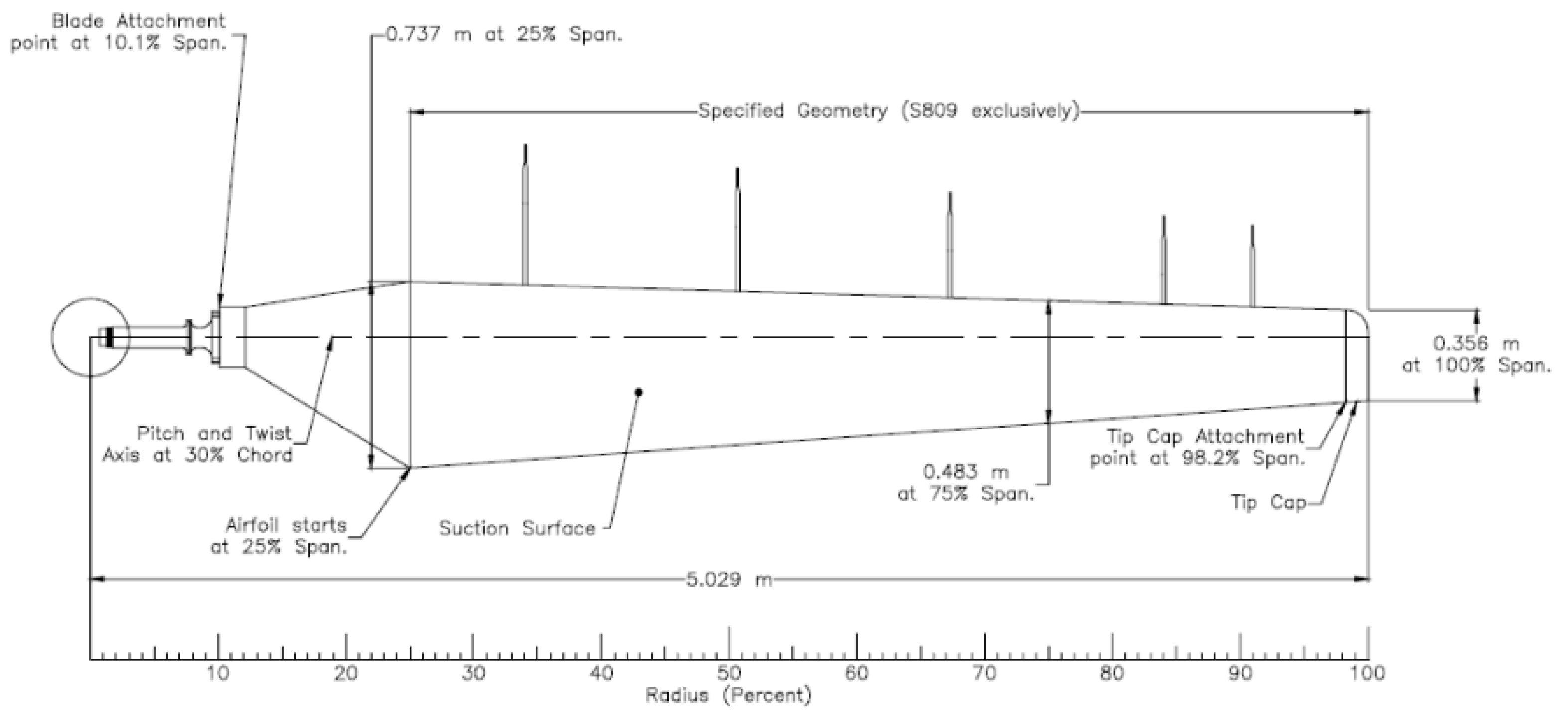
The geometry of the NREL Phase VI wind turbine was generated in SolidWorks 2019, concerning the dimensions from the work of Abate et al. [31], which is shown in Figure 2. The mesh was generated in OpenFOAM with the cylindrical fluid domain using BlockMeshDict. The fluid domain includes both a cylindrical outer domain and a cylindrical domain for the Arbitrary Mesh Interface (AMI) zone. The specifications for the outer domain were: (1) diameter = 100 m and length = 150 m; (2) for the Multiple Reference Frame (MRF)/AMI domain, the dimensions were a diameter of 20 m and a length of 26 m.

Creating a high-quality mesh is one of the most important and challenging tasks in Computational Fluid Dynamics (CFD) to ensure accurate and reliable results. Consequently, Pointwise was used for mesh generation around the NREL Phase VI wind turbine, as it is capable of producing structurally hyperbolic boundary layers tailored for the turbine. Additionally, a hybrid mesh approach, combining structured and unstructured techniques, was implemented for mesh creation, excluding the boundary layers around the turbine blades. The generated meshes for the fluid domain and blades are illustrated in Figure 3 and Figure 4, respectively.

In this simulation, a wind speed of 10 m/s and 72 rpm for blade rotation were applied. As mentioned above, the VLES model is used as a turbulence model in this simulation.

Table 1. Boundary conditions for the simulation.

Boundary Conditions	k	nut	omega	P	U
Inlet	FixedValue	zeroGradient	FixedValue	zeroGradient	FixedValue
Outlet	zeroGradient	zeroGradient	zeroGradient	slip	zeroGradient
Cylinder	slip	nutkWallFunction	omegaWallFunction	zeroGradient	slip
Propeller MRF	kqRWallFunction	nutkWallFunction	omegaWallFunction	zeroGradient	fixedValue
Propeller AMI	cyclicAMI	cyclicAMI	cyclicAMI	cyclicAMI	cyclicAMI
AMI1	cyclicAMI	cyclicAMI	cyclicAMI	cyclicAMI	cyclicAMI
AMI2	cyclicAMI	cyclicAMI	cyclicAMI	cyclicAMI	cyclicAMI

represents the applied boundary conditions in the CFD solver.

The boundary conditions play a crucial role in obtaining accurate results for CFD in wind turbine aerodynamics. The inlet and outlet boundaries for turbulence and velocity are specified as FixedValue and zeroGradient, respectively. The cylinder, which reflects the fluid domain, is defined by a slip boundary for kinematic conditions and a nutkWallFunction for the turbulent viscosity model. For the propeller, specified boundary conditions include kqRWallFunction and omegaWallFunction to simulate turbulence close to the rotor blades properly. The propeller and its two interfaces, AMI bounds, are modeled using cyclicAMI, which allows the adjacent domains to be coupled with a periodic boundary condition. These conditions enable the simulation to be predictive of the complex interplay between the fluid and structure while remaining computationally efficient, allowing the simulations to be performed for turbine operation under different operating conditions.

Mesh convergence analysis is a key part of numerical simulation that evaluates how mesh refinement impacts the accuracy of results. This is carried out by progressively refining the mesh and noting how the error decreases with each step.

Table 2. Mesh convergence study.

Mesh	No. 1	No. 2	No. 3	No. 4
Number of cells	17,131,110	24,078,878	36,932,383	54,937,248
Error (%)	10.1	8.22	3.86	0.9
CPU time (h)	254.6	365.2	602.5	950.3

shows the number of cells and corresponding errors for four different mesh resolutions. The number of cells increases from Mesh No. 1 to Mesh No. 4. This aligns with typical behavior, as increasing mesh refinement results in more cells in the simulation. A finer mesh generally better captures the physics of the model. For Mesh No. 1, the relative error was 10.1%, while for Mesh No. 4, it dropped significantly to 0.9%. This decrease in error highlights that mesh refinement is essential for improving the accuracy of computational models. However, finer meshes require more computational resources. Therefore, a balance must be struck between achieving higher accuracy and managing computational load.

3.2. Structural Model

The structural configuration of the NREL Phase VI wind turbine blade aims to develop a shell model compatible with the TACS structural solver. This shell model, shown in Figure 5, accurately represents the geometry of the entire blade, including the spar, and has been constructed to capture the most significant features that influence its response to wind loads. It serves as the primary geometric and structural element running through the blade, ensuring enhanced bridging stiffness and strength. Explicitly designed for stress and buckling analysis, this shell model enables the solver to simulate the mechanical response of the blade effectively. The structural mesh of the model is illustrated, with the blade discretized into finite elements represented by a blue mesh. This mesh is necessary to calculate the structural equations and forms part of the overall fluid-structure interaction (FSI) simulation, which couples fluid mechanics to the structural behavior of the blade during a TACS/DAFoam FSI simulation. The finer grid enables more realistic deformation and stress fields, leading to a better finite element analysis of the blade’s behavior under service conditions.

Table 3. Material properties for the structure of the blades.

Property	Symbol	Value	Unit
Density	ρ	2780.0	kg/m3
Elastic modulus	E	73.1 × 109	Pa
Poisson’s ratio	ν	0.33	—
Shear correction	k_corr	5.0/6.0	—
Yield stress	σ_y	324.0 × 106	Pa

shows the input parameters used for the shell model blades in the TACS solver. They ensure accurate predictions of blade deflection, stress distributions, and failure modes under both aerodynamic and gravitational loads. Utilizing these parametric values, the TACS solver computes the equations of motion, thereby assessing structural integrity through linear and nonlinear static and dynamic analyses.

In

Table 4. Shell thickness parameters.

Parameter	Symbol	Value	Unit
Nominal thickness	t	0.010	m
Minimum thickness	t_min	0.002	m
Maximum thickness	t_max	0.050	m

, the shell thickness (t) was defined as a constant baseline value of 0.010 m, with corresponding minimum and maximum allowable thicknesses of t_min = 0.002 m and t_max = 0.050 m, respectively, to allow for local variations and enable parametric investigation.

4. Results and Discussion

Figure 6 shows the convergence history of the pressure residuals during the transient FSI simulation of the NREL Phase VI wind turbine blade. The convergence criteria were established in the fvSolution dictionary within the OpenFOAM framework for ensuring accuracy and stability. The pimpleFoam solver was used to monitor the solution convergence via the residualControl settings. The residual thresholds of 10⁻⁵ and 10⁻⁶ without relative tolerance were imposed for the continuity and momentum equations, respectively. These equations were solved using the pressure field (p) and velocity field (U), respectively. The number of maximum iterations was set to 150 iterations per step for robust convergence without excessive computational cost. For the overall view (Figure 6a), it is seen that the residuals of the equations for a considerable number of time steps remain confined between 10⁻⁴ and 10⁻², allowing for the maintenance of numerical stability during the transient simulation. Such boundedness is crucial for the stability of the coupled solver, especially under the high-fidelity, time-resolving conditions involved in transient aeroelastic simulations. The zoomed view in Figure 6b depicts the residual evolution on a finer time scale, exhibiting an explicit periodic nature. This period is comparable to the unsteady aerodynamic loading and the structural deformations caused by the blade in one physical time step. The rapid decrease and subsequent increase in the residual values, which occur in each cycle, indicate that the solver can drive the residuals to smaller values in each inner iteration loop, thereby achieving convergence at each level in every time step. The lack of divergence and sudden peaks in the residuals also confirm the robustness and accuracy of the partitioned coupling method used in this FSI framework.

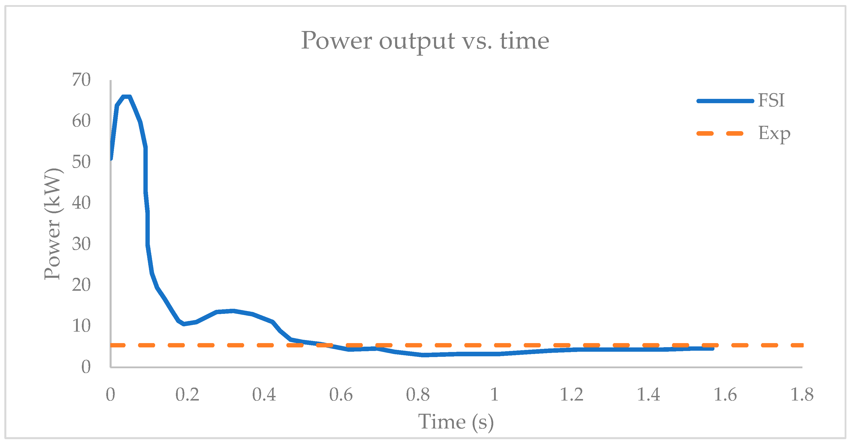
The power obtained from the FSI computation is plotted in Figure 7. The power output is shown as a function of time over a range from 0 to 1.8 s of simulation, with the FSI simulation results represented as a solid line and the steady-state power output as a horizontal dashed line taken from Lee et al. [3]. The simulation output shows a sharp peak during the early stage of the simulation at around 65 kW. This first overshoot is attributed to startup conditions and the rapid aerodynamic loading on the turbine blades. Then the power drops quickly, mainly due to blade deformation and aerodynamic damping as the system transitions to a steady state. From 0.1 to 0.8 s, the output power decreases significantly, falling below 10 kW and reaching a minimum near 2 kW. This phase corresponds to the transient dynamic response, during which structural vibrations and fluid-structure interaction effects become dominant, temporarily reducing the energy extracted from the flow. The power stabilizes after 0.8 s with slight oscillations around the nominal power output of 5 kW. This convergence toward steady-state power demonstrates the FSI simulation’s ability to accurately capture aeroelastic effects and the steady aerodynamic performance of the wind turbine. The results show that although transient effects cause notable power fluctuations during startup, the coupled fluid-structure model successfully predicts the turbine’s steady operational power. These findings align with previous experimental and numerical studies on the NREL Phase VI turbine, confirming the validity of the FSI simulation approach for detailed wind turbine performance analysis.

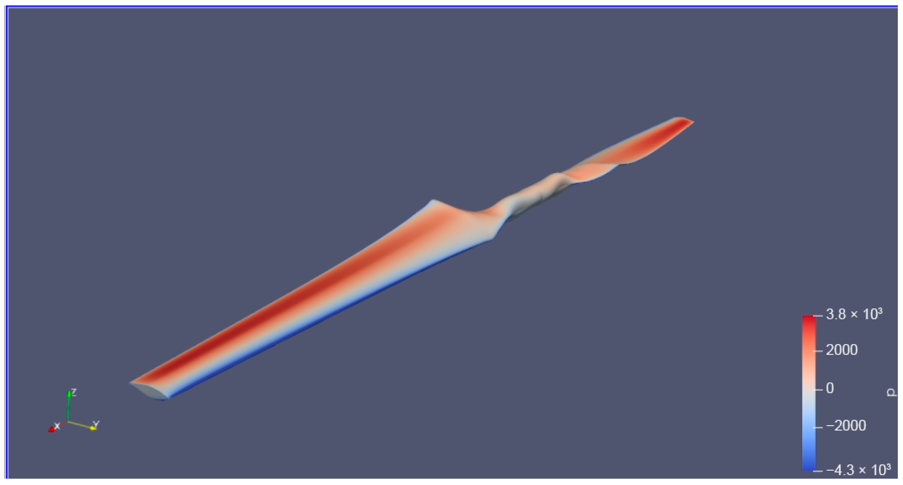
The pressure distribution over the blade surfaces is shown in Figure 8, illustrating how forces act on the wind turbine blades during operation. The figure highlights areas of high and low pressure, with red regions representing higher pressure and blue regions indicating lower pressure. The pressure gradient is essential for predicting the aerodynamic and structural performance of the blade. Additionally, pressure differences can significantly impact the efficiency, lifespan, and wear of the blades.

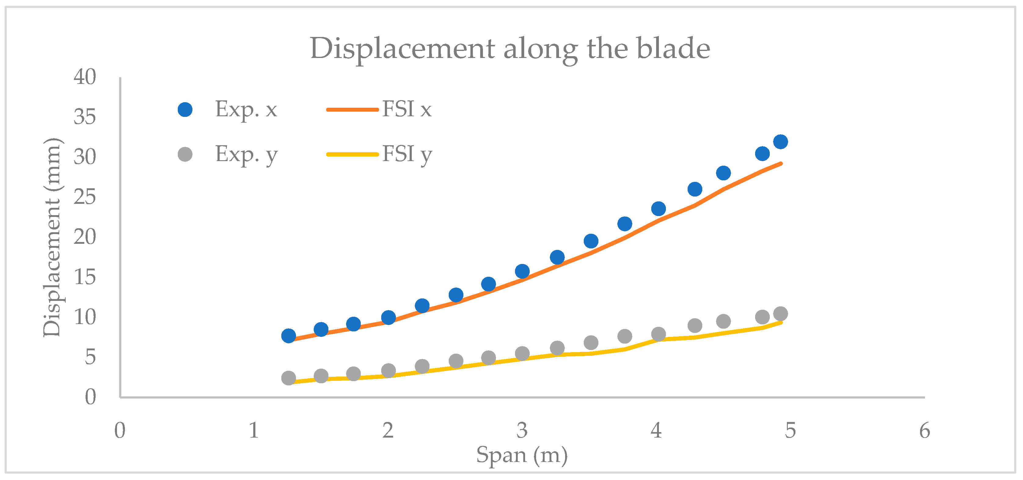
The blade displacement data were obtained from FSI simulations, as shown in Figure 9. Displacement is depicted as two lines along the blade span, representing displacement in the x and y directions. The graph compares the simulated displacement with experimental data. The experimental results closely match the FSI simulation outcomes, particularly in the x direction, confirming the accuracy of the simulation model in predicting turbine blade deformation under operational conditions [3].

Figure 10 illustrates the comparison of time histories for blade tip displacement derived from both fluid-structure interaction (FSI) simulations and experimental data. The simulation reveals rapid, albeit small-scale oscillations in the displacement over time, characterized by an impulsive transient response that stabilizes quickly. The FSI-predicted tip displacement converges to approximately 0.0295 m, which aligns closely with the experimental measurement of 0.03 m. This slight underestimation of about 1.7% in the simulation may be attributed to various modeling assumptions, such as material damping, boundary conditions, or turbulence modeling. The initial transient response observed was anticipated due to the sudden increase in aerodynamic loading at the beginning of the simulation. Overall, the strong correlation between the simulation results and experimental data indicates that the developed coupled model effectively predicts the dynamic deformation properties of the wind turbine blade during operation [3].

In Figure 11, the simulated pressure coefficient (Cp) data were compared and discussed at four radial locations: r/R = 30%, 46.6%, 63%, and 95%. These results were systematically compared to experimental data from the study by Hsu et al. [32] to validate the accuracy and fidelity of the simulation model. As shown in Figure 8, the Cp curves along the normalized chord length (x/c) have aerodynamic features according to the loading on the blade sections. At midspan (r/R = 30%), it is reported that the simulation predicts a strong suction peak around the leading edge of the suction side, and Cp is in good agreement with the CP experiment for the case of Cp. On the pressure side, the pressure gradient is relatively smooth, with a slight underprediction of Cp around the trailing edge by the simulation. This suggests the model is effectively capturing the flow behavior in the high-loading inner blade region. Very good agreement with the experiment is maintained at the midspan stations (r/R = 46.6% and 63%) for FSI results. The leading-edge suction peaks are well captured, and downstream, the pressure distributions on both the suction and pressure sides match experimental trends well. Only small differences can be observed for the mid-chord region, in which Cp is perhaps slightly overestimated by the simulation, due to turbulence model performance or grid resolution. Close to the blade tip (r/R = 95%), the Cp distributions represent a more complicated phenomenon in flow. The leading-edge suction peak and the general pressure distribution are captured well by the simulation, but some discrepancies exist near the trailing edge. These differences are likely to be attributed to unsteady flow separation or vortex dynamics, which are difficult to capture in the current numerical framework accurately. In general, the FSI simulation exhibits good predictive ability for aerodynamic pressure distributions over the blade span. The close agreement between the prediction and the experimental results from the literature verifies the methodology. It indicates that it may be used for detailed aerodynamic and structural analyses in wind turbine blade design.

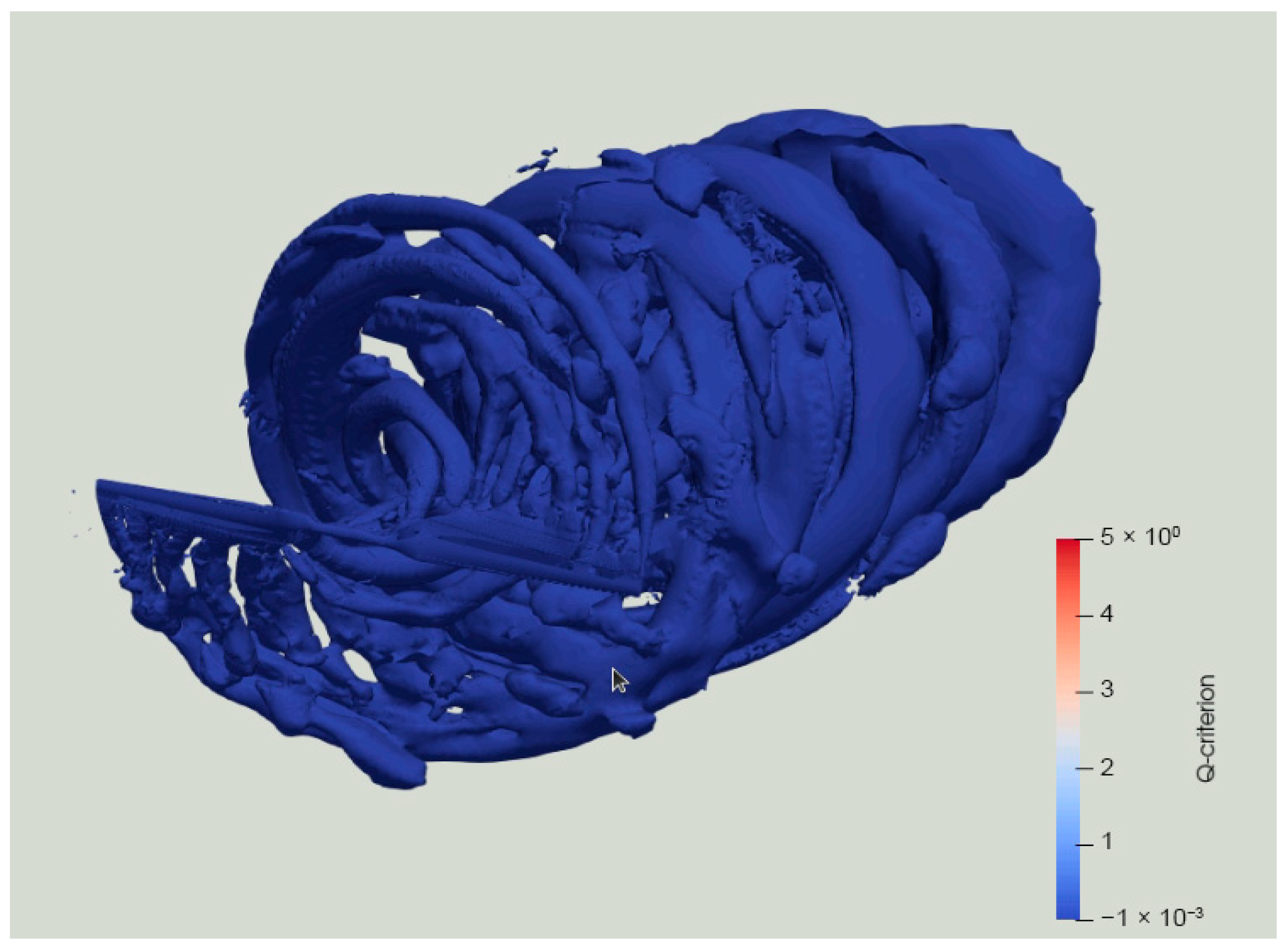
The investigation of the wake characteristics of wind turbine blades is important to understand the aerodynamic performance of wind turbines under different ambient flow conditions. The wake structure obtained from the FSI simulation is presented in Figure 12, providing a decomposition of the intricate relationship between the flow field and the turbine blades. The wake pattern in the figure illustrates the turbulence and flow characteristics generated as the blades of the wind turbines pass through the air. These flow structures will be pivotal in evaluating the influence of vortex shedding and turbulence interaction with the surrounding flow field. It can be seen from Figure 12 that vortex cores are generated and swept back over the blade trailing edge; this has a significant impact on the energy collection effectiveness and stability of the wind turbine blades.

5. Conclusions

This study provides a detailed investigation of the high-fidelity, two-way FSI simulation of wind turbines with the Arbitrary Hybrid Turbulence Model (AHTM). The use of the VLES in the DAFoam solver, together with the TACS structural solver, represents an unprecedented platform for wind turbine modeling, providing a new tool for turbine performance and structural integrity assessment under dynamic loads. Results show that the advanced turbulence models and FSI lead to better predictions of power, blade deformation, and aerodynamic performance compared to conventional methods. The paper helps in understanding the significance of taking into account complex flow-structure interaction, especially in large-scale wind turbines, where the BEM-based models are unable to do so. Furthermore, the simulation results are in good agreement with experimental data, proving the predictive capability of the model regarding the actual behavior of the turbines. While the simulation was carried out to satisfaction, the experimentalist acknowledges the computational complexities of accurate high-fidelity simulations and the importance of controlling the amount of computational effort used to achieve responses of tolerable accuracy. Although the current work showed the capability of the high-fidelity FSI simulation of the 2-bladed NREL Phase VI wind turbine, additional validation cases can be pursued in future studies. In particular, the bladed MEXICO rotor provides a useful reference case for comparison as it is well documented, and the full span transient flow field has been made available. Following the same high-fidelity approach to the MEXICO-test-rotor would provide a more extensive comparison of the proposed framework and additionally enable validation over a wider operational envelope and rotor types. Such a study would yield some interesting approximate solutions and could help to better understand the aerodynamic and structural response of modern multi-blade propellers under realistic loadings. To conclude, this work offers significant advances in the understanding of wind turbine dynamics, which is an essential source of information for conducting further improved and robust innovative designs related to wind energy harvesting. The advanced turbulence models and FSI simulations-based coupling constitute a stepping stone for further advances in wind turbine technology, guaranteeing higher performance and more extended durability in various operating environments.

References

1. Ren, Z.; Verma, A.S.; Li, Y.; Teuwen, J.J.; Jiang, Z. Offshore wind turbine operations and maintenance: A state-of-the-art review. Renew. Sustain. Energy Rev. 2021, 144, 110886. [Google Scholar] [CrossRef]
2. Lee, Y.J.; Jhan, Y.T.; Chung, C.H. Fluid–structure interaction of FRP wind turbine blades under aerodynamic effect. Compos. Part B Eng. 2012, 43, 2180–2191. [Google Scholar] [CrossRef]
3. Lee, K.; Huque, Z.; Kommalapati, R.; Han, S.E. Fluid-structure interaction analysis of NREL phase VI wind turbine: Aerodynamic force evaluation and structural analysis using FSI analysis. Renew. Energy 2017, 113, 512–531. [Google Scholar] [CrossRef]
4. Hewitt, S.; Revell, A.; Margetts, L. A Novel Black-Box Massively Parallel Partitioned Approach to Fluid-Structure Interaction Problems. In Proceedings of the 24th UK Conference of the Association for Computational Mechanics in Engineering, Cardiff, UK, 31 March–1 April 2016. [Google Scholar]
5. Xu, Z.; Wei, J.; Zhang, S.; Liu, Z.; Chen, X.; Yan, Q.; Guo, J. A state-of-the-art review of the vibration and noise of wind turbine drivetrains. Sustain. Energy Technol. Assess. 2021, 48, 101629. [Google Scholar] [CrossRef]
6. Kim, D.H.; Lim, O.; Choi, E.H.; Noh, Y. Optimization of 5-MW wind turbine blade using fluid structure interaction analysis. J. Mech. Sci. Technol. 2017, 31, 725–732. [Google Scholar] [CrossRef]
7. Zhangaskanov, D.; Batay, S.; Kamalov, B.; Zhao, Y.; Su, X.; Ng, E.Y.K. High-Fidelity 2-Way FSI Simulation of a Wind Turbine Using Fully Structured Multiblock Meshes in OpenFoam for Accurate Aero-Elastic Analysis. Fluids 2022, 7, 169. [Google Scholar] [CrossRef]
8. Guma, G.; Bucher, P.; Letzgus, P.; Lutz, T.; Wüchner, R. High-fidelity aeroelastic analyses of wind turbines in complex terrain: FSI and aerodynamic modelling. Wind. Energy Sci. Discuss. 2022, 7, 1421–1439. [Google Scholar] [CrossRef]
9. Kamalov, B.; Batay, S.; Zhangaskhanov, D.; Zhao, Y.; Ng, E.Y.K. Arbitrary Hybrid Turbulence Modeling (AHTM) Approach for High Fidelity NREL Phase VI Wind Turbine CFD Simulation. Fluids 2022, 7, 236. [Google Scholar] [CrossRef]
10. Grinderslev, C.; González Horcas, S.; Sørensen, N.N. Fluid structure interaction simulation of a wind turbine rotor in complex flows, validated through field experiments. Wind Energy 2021, 24, 1426–1442. [Google Scholar] [CrossRef]
11. Bazilevs, Y.; Takizawa, K.; Tezduyar, T.E.; Hsu, M.C.; Kostov, N.; McIntyre, S. Aerodynamic and FSI analysis of wind turbines with the ALE-VMS and ST-VMS methods. Arch. Comput. Methods Eng. 2014, 21, 359–398. [Google Scholar] [CrossRef]
12. Wang, L.; Quant, R.; Kolios, A. Fluid structure interaction modelling of horizontal-axis wind turbine blades based on CFD and FEA. J. Wind. Eng. Ind. Aerodyn. 2016, 158, 11–25. [Google Scholar] [CrossRef]
13. Santo, G.; Peeters, M.; Van Paepegem, W.; Degroote, J. Fluid–structure interaction simulations of a wind gust impacting on the blades of a large horizontal axis wind turbine. Energies 2020, 13, 509. [Google Scholar] [CrossRef]
14. Shi, F.; Wang, Z.; Zhang, J.; Gong, Z.; Guo, L. Influences of wind and rotating speed on the fluid-structure interaction vibration for the offshore wind turbine blade. J. Vibroeng. 2019, 21, 483–497. [Google Scholar] [CrossRef]
15. Deng, Z.; Xiao, Q.; Huang, Y.; Yang, L.; Liu, Y. A general FSI framework for an effective stress analysis on composite wind turbine blades. Ocean. Eng. 2024, 291, 116412. [Google Scholar] [CrossRef]
16. Gray, J.S.; Hwang, J.T.; Martins, J.R.R.A.; Moore, K.T.; Naylor, B.A. OpenMDAO: An open-source framework for multidisciplinary design, analysis, and optimization. Struct. Multidiscip. Optim. 2019, 59, 1075–1104. [Google Scholar] [CrossRef]
17. Lafage, R.; Defoort, S.; Lefebvre, T. WhatsOpt: A web application for multidisciplinary design analysis and optimization. In Proceedings of the AIAA Aviation 2019 Forum, Dallas, TX, USA, 17–21 June 2019; p. 2990. [Google Scholar]
18. Moukalled, F.; Mangani, L.; Darwish, M. The Finite Volume Method in Computational Fluid Dynamics; Springer: Cham, Switzerland, 2016; Volume 113. [Google Scholar] [CrossRef]
19. Ridzuan, F.; Manshoor, B.; Omar, M.H.; Didane, D.H.; Abdelaal, M.A.; Amin, A. Aerodynamic Performance of NACA S809 Wind Turbine Blade Airfoil Using SST K-omega and K-epsilon Turbulence Models. J. Des. Sustain. Environ. 2024, 6, 36–42. [Google Scholar]
20. Tachos, N.S.; Filios, A.E.; Margaris, D.P. A comparative numerical study of four turbulence models for the prediction of horizontal axis wind turbine flow. Proc. Inst. Mech. Eng. Part C J. Mech. Eng. Sci. 2010, 224, 1973–1979. [Google Scholar] [CrossRef]
21. Nichols, R. Applications of RANS/LES turbulence models. In Proceedings of the 41st Aerospace Sciences Meeting and Exhibit, Reno, NV, USA, 6–9 January 2003; p. 83. [Google Scholar]
22. Taghinia, J.H.; Rahman, M.M.; Siikonen, T. A sub-grid scale model with natural near-wall damping. Aerosp. Sci. Technol. 2018, 74, 1–16. [Google Scholar] [CrossRef]
23. Maulenkul, S.; Yerzhanov, K.; Kabidollayev, A.; Kamalov, B.; Batay, S.; Zhao, Y.; Wei, D. An Arbitrary Hybrid Turbulence Modeling Approach for Efficient and Accurate Automotive Aerodynamic Analysis and Design Optimization. Fluids 2021, 6, 407. [Google Scholar] [CrossRef]
24. Stephens, D.; Sideroff, C.; Jemcov, A. A two equation VLES turbulence model with near-wall delayed behaviour. In Proceedings of the 7th Asia-Pacific International Symposium on Aerospace Technology, Cairns, QC, Australia, 25–27 November 2015; Volume 10. [Google Scholar]
25. Tiwari, P.; Xia, Z.; Han, X. Comparison of VLES and LES turbulence modeling for swirling turbulent flow. J. Appl. Fluid Mech. 2020, 13, 1107–1116. [Google Scholar] [CrossRef]
26. Liu, D.; Tang, W.; Wang, J.; Xue, H.; Wang, K. Comparison of laminar model, RANS, LES and VLES for simulation of liquid sloshing. Appl. Ocean. Res. 2016, 59, 638–649. [Google Scholar] [CrossRef]
27. Mangani, L.; Buchmayr, M.; Darwish, M.; Moukalled, F. A fully coupled OpenFOAM® solver for transient incompressible turbulent flows in ALE formulation. Numer. Heat Transf. Part B Fundam. 2017, 71, 313–326. [Google Scholar] [CrossRef]
28. Zhao, Y.; Su, X. Arbitrary Lagrangian–Eulerian (ALE) Method and Fluid-Structure Interaction. In Computational Fluid-Structure Interaction; Elsevier: Amsterdam, The Netherlands, 2019; pp. 127–144. [Google Scholar] [CrossRef]
29. Issa, R. Solution of the implicit discretized fluid flow equations by operator splitting. J. Comput. Phys. 1986, 62, 40–65. [Google Scholar] [CrossRef]
30. Beam and Shell Elements in TACS—TACS Documentation. Available online: https://smdogroup.github.io/tacs/theory/shell_element.html (accessed on 25 May 2025).
31. Abate, G.; Mavris, D.N.; Sankar, L.N. Performance effects of leading edge tubercles on the NREL Phase VI wind turbine blade. J. Energy Resour. Technol. 2019, 141, 051206. [Google Scholar] [CrossRef]
32. Hsu, M.-C.; Akkerman, I.; Bazilevs, Y. Finite element simulation of wind turbine aerodynamics: Validation study using NREL Phase VI experiment. Wind. Energy 2014, 17, 461–481. [Google Scholar] [CrossRef]
Figure 1. The flowchart for FSI framework [17].
Energies 18 04401 g001
Figure 2. Dimensions for NREL Phase VI wind turbine [31].
Energies 18 04401 g002
Figure 3. (a) Fluid domain mesh. (b) Rotating zone mesh inside the fluid domain.
Energies 18 04401 g003
Figure 4. Blades mesh inside the fluid domain. (a) General view; (b) Closer view.
Energies 18 04401 g004
Figure 5. Shell model for structural solver. (a) Shell model structure; (b) Shell model mesh.
Energies 18 04401 g005
Figure 6. Residuals of pressure versus number of iterations graph. (a) General view; (b) Expanded view.
Energies 18 04401 g006
Figure 7. Comparison of power output versus time graphs from the simulation and experiment.
Energies 18 04401 g007
Figure 8. Pressure distribution on the blades.
Energies 18 04401 g008
Figure 9. Displacement in the x and y directions comparison from the simulation and experiment.
Energies 18 04401 g009
Figure 10. Comparison of FSI simulation and experimental blade tip displacement over time.
Energies 18 04401 g010
Figure 11. Power coefficients for FSI simulation and experiment.
Energies 18 04401 g011
Figure 12. Wake structure from the FSI simulation.
Energies 18 04401 g012