Article

Distribution Network Situational Awareness Prediction Based on Spatio-Temporal Attention Dynamic Graph Neural Network

1
School of Microelectronics and Communication Engineering, Chongqing University, Chongqing 401331, China
2
State Grid Zhejiang Electric Power Co., Ltd., Hangzhou 311000, China
*
Author to whom correspondence should be addressed.
Energies 2025, 18(16), 4402; https://doi.org/10.3390/en18164402
Submission received: 18 July 2025 / Revised: 14 August 2025 / Accepted: 15 August 2025 / Published: 18 August 2025
(This article belongs to the Section A1: Smart Grids and Microgrids)

Abstract

Distribution network situational awareness prediction is a key technology for ensuring the safe and stable operation of distribution networks. However, most existing methods suffer from spatio-temporal dynamic correlation and dynamic topology, resulting in unsatisfactory performance. To address these issues, we propose a distribution network situational awareness prediction method based on a spatio-temporal attention dynamic graph neural network model that realizes the decoupling of spatio-temporal features of the distribution network data by adopting the alternating stacking of the multi-head self-attention mechanism with temporal dynamic perception and the spatial dynamic graph convolution module. Furthermore, the dynamic correlation matrix is introduced to adaptively adjust the node interaction weights to effectively handle the network dynamic topology information. Through extensive experiments, the proposed method outperforms eight baseline models.

1. Introduction

Situational awareness of the security of the distribution network is a key technology for comprehensively and dynamically analyzing the security operation state and potential hazards of distribution networks, especially in the high proportion of renewable energy situations [1,2,3]. It is a difficult task to accurately and comprehensively predict the operation situation of the distribution network. Recently, machine learning and deep learning algorithms have been used in predicting distribution network security situational awareness due to their excellence in solving complex nonlinear problems. Tian [4] uses a long short-term memory (LSTM) network to predict the time series of trends in distribution network operation to realize the perception of future and real-time state security risks of distribution networks. Xie [5] proposes a long short-term memory network combined with an attention mechanism (LSTMA) method, using LSTM to mine time-series information, while introducing an attention mechanism to highlight important information in time-series samples, thus achieving a transient stability assessment of power systems. Xu [6] proposes a method for predicting the situation of distribution networks based on temporal pattern attention–bidirectional long short-term memory (TPA-BiLSTM). By processing input sequences in both forward and reverse directions, the model can simultaneously obtain information before and after the current time step, and the introduction of the TPA attention mechanism enables the model to focus on key information at different time steps, further enhancing the accuracy of time-series data analysis. Luo [7] proposes a method for the situation awareness of distribution networks based on empirical mode decomposition (EMD), singular value decomposition (SVD), and Elman neural networks. It predicts the operating situation of distribution networks through Elman neural networks and combines a comprehensive evaluation method of fragile nodes to identify and evaluate fragile nodes, thereby improving the accuracy of situational awareness. Despite the progress made, most of the existing methods focus on assessing and predicting the current operating status of distribution networks, without assessing and predicting future conditions. At the same time, the following challenges have not been resolved.
  • Insufficient exploration of spatio-temporal dynamic correlations. Distribution networks are complex systems with spatio-temporal coupling, whose operation state not only changes over time but is also affected by spatial location. However, most existing methods [4,5,6,7] only consider the time-series dimension of distribution network data and fail to fully consider the spatial correlations of distribution networks. Neglecting the spatio-temporal dynamic correlations will result in the model being unable to comprehensively capture the operating patterns of distribution networks, thereby affecting the accuracy of the prediction.
  • Insufficient adaptability of dynamic topology structures. Distribution networks are subject to complex and variable loads and faults, and dynamic changes in topology structures (such as fault disconnections, additional loads, equipment maintenance, etc.) may occur at any time [8]. It is difficult for traditional modeling methods based on fixed topology structures to adapt to such dynamic changes, and they cannot accurately reflect the actual operation state of distribution network.
In recent years, spatio-temporal graph neural networks have been widely applied to the prediction of transportation, environment, safety, energy, and other fields, combine spatial and temporal dimensions for feature processing, and are suitable for dynamic graph topology. Guo [9] proposes a spatio-temporal graph convolutional network model that can simultaneously consider time-series data and spatial structure information and achieves good results in traffic flow prediction. Khodayar [10] proposes a spatio-temporal graph deep neural network for short-term wind speed prediction that combines LSTM and graph convolutional networks to capture the spatio-temporal characteristics of wind power and improve wind speed prediction accuracy. Simeunović [11] proposes a graph convolutional long and short-term memory network (GCLSTM) and graph convolutional transformer (GCTrafo) model that can effectively explore the spatio-temporal correlations in the photovoltaic data and realize the high-precision prediction of multi-site photovoltaic power. Li [12] proposes an STDGCNN model for ultra-short-term wind power prediction that can effectively explore the spatio-temporal dependence between wind power through the construction of directed graphs and the improvement of graph convolutional layers. Zhang [13] proposes a model based on a graph attention mechanism and bi-directional LSTM for the short-term load forecasting of virtual power plants that can effectively capture the spatial and time-series features of the load data of virtual power plants by combining GAT and bi-directional LSTM.
Although spatio-temporal graph neural networks have been applied in tasks such as wind speed prediction, photovoltaic power prediction, and load forecasting in the energy field, they are underutilized in this aspect of distribution network security posture prediction. Based on this and the above mentioned shortcomings of existing distribution network posture prediction methods, this paper proposes a method for predicting and evaluating the security state of distribution networks based on the spatial–temporal attention dynamic graph neural network (STADGNN) model to achieve an accurate perception and prediction of the future status of the distribution network based on historical data, which adopts a spatial–temporal dynamic correlation model to achieve decoupling of spatial–temporal features through the alternating stacking of the multi-head self-attention mechanism with temporal dynamic perception and the spatial dynamic graph convolution module. Meanwhile, a dynamic correlation matrix is introduced to adaptively adjust the node interaction weights, effectively processing network dynamic topology information.
The remainder of this paper is summarized as follows. Section 2 first introduces the composition of the security situation awareness prediction system model and then details the core modules of the proposed STADGNN model and the distribution network situation awareness prediction process. Section 3 defines the power distribution network security situation assessment index indicators, sets the simulation verification experimental parameters and datasets, and then discusses the experimental results, analyzes the performance of the proposed model in different situations, and compares it with existing methods. Finally, Section 4 summarizes the paper and proposes suggestion for future research.

2. The Security Situational Awareness System Model

As shown in Figure 1, the security situational awareness system model mainly includes two parts: the distribution network graph model and the STADGNN model.

2.1. Distribution Network Graph Model

The nodes and lines of the distribution network can form a natural graph [14]. In this paper, we model the STADGNN model from a graph perspective for distribution network security situational awareness prediction. At the same time, since the operation of distribution networks changes over time, a distribution network graph model is constructed to represent the spatial relationships between electrical equipment in distribution networks and their power state changes over time.
The distribution network is defined as an undirected graph G = V , E , A , where V is a set of nodes V = N , and each node represents a power equipment or monitoring point, such as a substation, the end of a distribution line, a distribution transformer, a load monitoring device, etc. The features of each node include data such as the voltage and current of the equipment, which vary over time. E is the set of edges E = M , where each edge represents a transmission line or feeder, constructed based on the physical topology of the power grid. A R N × N is the adjacency matrix of the graph G, which represents the adjacency relationships between nodes.
The observed monitoring values of the distribution network G during the t t h time interval are represented by the signal matrix X t = ( x t , 1 , x t , 2 , , x t , N ) T R N × C , where x t , ν R C denotes the value of the feature quantity of node v within the t t h time interval and C denotes the number of features. The features of the node are not only the current power state but also the time-series data, such as the voltage and current of the equipment over a period of time in the past, reflecting the dynamic changes in the distribution network.

2.2. STADGNN Model

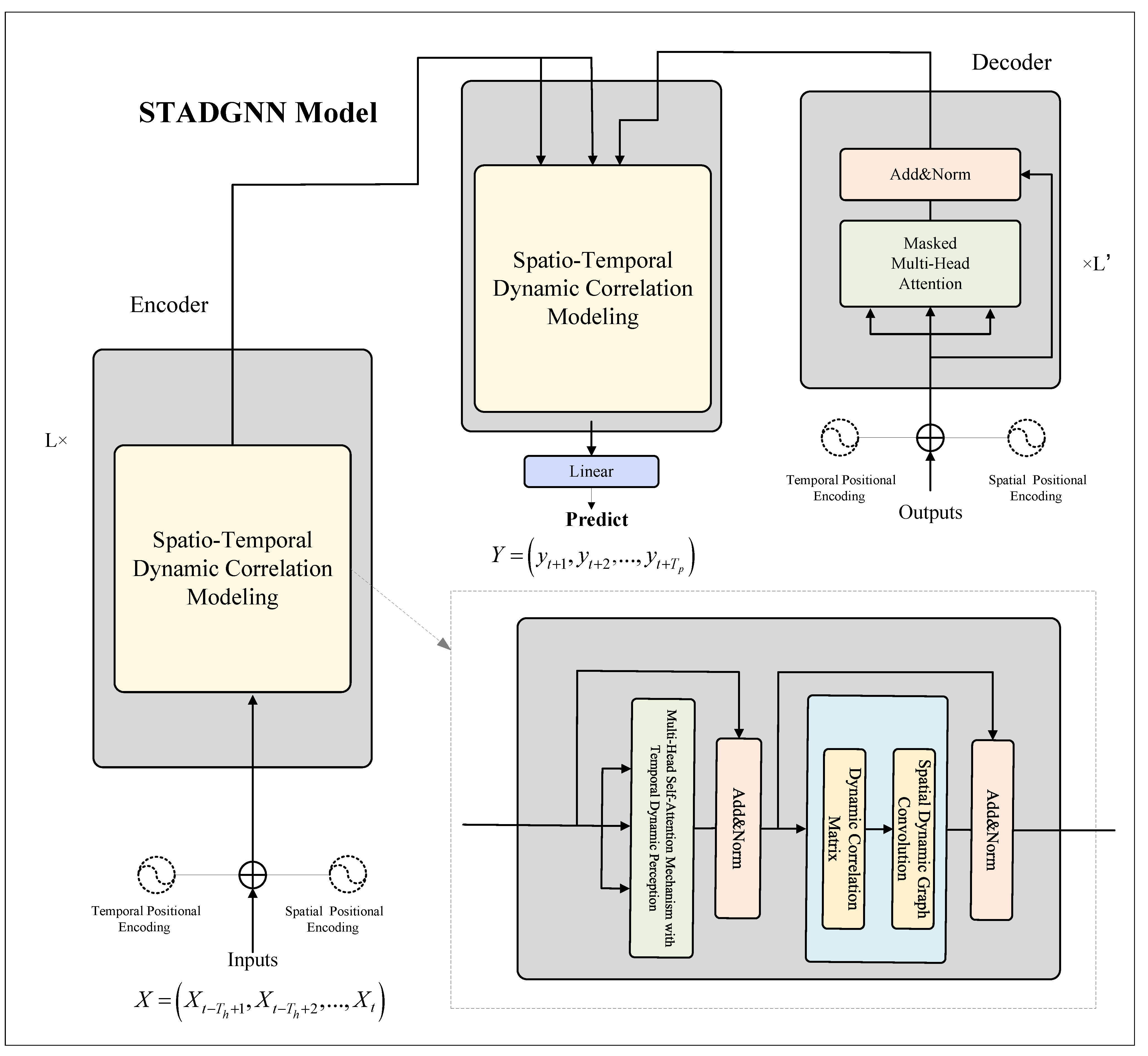
Inspired by the success of the transformer model [15] in the field of natural language processing, the STADGNN model proposed in this paper is based on the self-attention mechanism and adopts an encoder–decoder architecture [16], as shown in Figure 2. Both the encoder layer and the decoder layer are stacked with spatio-temporal correlation modules. At the same time, in order to ensure that the model can maintain good training results when the number of layers increases, residual connections [17] and layer normalization [18] are introduced between layers. The encoder is responsible for processing the input spatio-temporal data and generating latent feature representations; the decoder outputs the security state prediction results of the distribution network based on these latent representations.
The input of the l t h encoder layer can be denoted as X ( l 1 ) = ( X t T h + 1 ( l 1 ) , X t T h + 2 ( l 1 ) , , X t ( l 1 ) ) R N × d model × T h , where l 1 , 2 , · · · , L , and the processing flow of the STADGNN model is as follows.
First, the initial input X R N × C × T h is converted into a high-dimensional feature space representation X ( 0 ) R N × d model × T h through linear projections by the temporal embedding layer and spatial embedding layer, where d model > C . Then, the encoder maps the input sequence X ( 0 ) = ( X t T h + 1 ( 0 ) , X t T h + 2 ( 0 ) , . . . , X t ( 0 ) ) to X ( L ) = ( X t T h + 1 ( L ) , X t T h + 2 ( L ) , , X t ( L ) ) through L encoder layers. The decoder part generates the future output sequence Y ( L ) = ( X t + 1 ( L ) , X t + 2 ( L ) , . . . , X t + T p ( L ) ) based on the encoder’s output X ( L ) and using another L decoder’s layers. Finally, Y ( L ) is mapped to the target output Y of a specified dimension through a linear projection.

2.2.1. Multi-Head Self-Attention Mechanism with Temporal Dynamic Perception

The traditional self-attention mechanism dynamically allocates weights to different positions by calculating the dot product relationship between the query, key, and value, which is calculated by the following formula:
A t t e n t i o n ( Q , K , V ) = s o f t max ( Q K T d m o d e l ) V
where Q, K, V, and d m o d e l are query, key, value, and feature dimensions, respectively.
The multi-head self-attention mechanism [15] is an extended form of the self-attention mechanism, which can capture global dependencies, but it has insufficient sensitivity to local trends when processing continuous time-series data. It relies only on dot product calculation, which makes it difficult to distinguish between data points with the same numerical values but differing local trends. For example, two time points with the same voltage value, one in a steady state and the other in a fluctuating peak caused by harmonic disturbances, may be incorrectly assigned similar weights by traditional self-attention. To address this issue of insufficient sensitivity to local trends, the proposed model adopts a multi-head self-attention mechanism with temporal dynamic perception that takes into account the local contextual information in which each data point is located, which is a variant of the convolutional self-attention mechanism [19]. It can effectively and accurately model the dynamic nature of distribution network data in the time dimension. In the convolutional self-attention mechanism, one-dimensional convolution is used to replace the linear projection of Q and K in the traditional self-attention mechanism. One-dimensional convolution kernels Φ j Q and Φ j K are applied to input sequences Q and K, respectively, to extract gradient information within the local window at each time point. The convolved features Q ˜ and K ˜ are defined as follows:
Q ˜ = Φ j Q Q
K ˜ = Φ j K K
where Φ j Q and Φ j K are parameters of the convolution kernel and “∗” denotes the convolution operation. The convolved features Q ˜ and K ˜ are input into the multi-head attention mechanism to calculate the dynamic weights, which are calculated as follows:
h e a d j = s o f t max Q ˜ K ˜ T d m o d e l V W j V
where h e a d j denotes the j t h temporal dynamic self-attention operation and W j V is the projection matrix that maps V to different representation subspaces. The final definition is obtained by splicing the multiple outputs through a linear transformation as follows:
Z ( l ) = C o n c a t ( h e a d 1 , . . . h e a d h ) W 0
where h is the number of attention heads and W 0 is the final output projection matrix.

2.2.2. Dynamic Correlation Matrix

It is difficult for traditional modeling methods based on fixed topology structures to adapt to dynamic changes in topology structures, and they cannot accurately reflect the actual operation state of the distribution network. In this paper, a dynamic correlation matrix is introduced to adaptively adjust the node interaction weights.
In the l t h layer of the encoder, given the input X ( l 1 ) , after executing the temporal dynamic awareness multi-head self-attention mechanism on all nodes, the output of the temporal dynamic awareness multi-head self-attention mechanism can be obtained, i.e., the intermediate representation of the node Z t ( l 1 ) R N × d model . Based on this node feature, the dynamic correlation matrix S t can be obtained and calculated as follows:
S t = s o f t max ( Z t ( l 1 ) Z t ( l 1 ) T d m o d e l ) R N × N
where S t i , j denotes the strength of association between nodes i and j at the moment t, which is determined by their feature similarity.

2.2.3. Spatial Dynamic Graph Convolution

Traditional graph convolutions [20] aggregate information based on a fixed topological structure, which is calculated as follows:
X ( l ) = σ ( A X ( l 1 ) W ( l ) )
where A is the static adjacency matrix that reflects the fixed connection relationships between nodes, and X t ( l 1 ) R N × d mod el , W ( l ) , σ are the node representations, projection matrices, and nonlinear activation functions, respectively.
However, spatial correlation changes dynamically in distribution networks and there are complex and variable loads and faults, with the possibility of dynamic changes in the topological structure at any time. Traditional graph convolution cannot adapt to such dynamic changes, so dynamic spatial correlation modeling needs to be introduced. This paper uses spatial dynamic graph convolution [21], which can correlate static topology with dynamic features and adaptively adjust the interaction weights between nodes. After obtaining the dynamic correlation matrix S t , it is combined with the static neighbor matrix A to generate the adaptive weights:
A ˜ t = A S t
where ⊙ denotes the Hadamard product (multiplication of elements by elements). Based on the adaptive weight A ˜ t , graph convolution is performed to update node features:
X t ( l ) = D G C N ( Z t ( l 1 ) ) = σ ( A ˜ t Z t ( l 1 ) W ( l ) )
From Equation (9), it can be seen that the dynamic graph convolution module integrates neighboring information based on the correlation matrix derived from the input Z ( l 1 ) . After passing through the spatial dynamic graph convolution module, a new spatial information output X ( l ) = ( X t T h + 1 ( l ) , X t T h + 2 ( l ) , , X t ( l ) ) R N × d m o d e l × T h is ultimately obtained.

2.2.4. Spatio-Temporal Position Embedding Module

Position embedding is a technique that encodes positional information and incorporates it into the model input. It is primarily used for processing sequence data. Position embedding is categorized into temporal position embedding and spatial position embedding.
Temporal position embedding can identify the absolute or relative position of data points in a time series. In the multi-head self-attention mechanism for temporal dynamic sensing, the dynamics are fully modeled by the self-attention mechanism. The self-attention mechanism itself is insensitive to the order of the input, and temporal proximity often plays a critical role in time-series modeling tasks. Therefore, in this paper, we add a temporal position embedding vector to each element in the sequence through temporal position embedding to ensure that adjacent elements have similar embeddings. Each dimension d 1 d d m o d e l of the position embedding vector of the element at position t is represented as follows:
E T P ( t , 2 d ) = sin ( t / 10000 2 d / d m o d e l )
E T P ( t , 2 d + 1 ) = cos ( t / 10000 2 d / d mod s l )
where t is the relative index of each element in the input. This representation helps the model to better capture the sequential information in the time series.
Spatial position embedding can identify the spatial position and attribute differences in nodes in the topology of the power grid, allowing the model to learn features of the position-based distribution network data. In order to reflect the information about the graph structure, an initial spatial position embedding matrix is obtained by first assigning an additional embedding vector E S P ( 0 ) R N × d model to each node. Then, the nodes are Laplace-smoothed by a graph convolution layer [22] to obtain the final spatial position embedding matrix E S P .
Finally, the temporal position embedding matrix E T P and spatial position embedding matrix E S P will be added to the original input representation X ( 0 ) , respectively.

2.3. Distribution Network Situational Awareness Based on the STADGNN Model

2.3.1. Distribution Network Security Situational Assessment Indicators

The construction of the distribution network security situational assessment indicators aims to monitor the security state of the distribution network and provide risk warnings by quantifying the basic parameters of the distribution network operation [23,24]. Specifically, it includes the following situational indicator values and comprehensive assessment values [25,26].
(1) Node voltage overturn margin:
Voltage index is an important indicator of the security state of the distribution network. Node voltage overturn will affect the stable operation of the distribution network. This paper uses node voltage overturn margin A 1 to represent the current tolerability of node voltage overturn, which is calculated as follows:
A 1 = 1 U i U a + U b 2 ( U a + U b ) 2
where U i , U a , and U b represent the voltage value, voltage upper limit, and voltage lower limit of the node i, respectively. In this paper, we select the standard values U a and U b as 1.05 and 0.95, respectively. When A 1 is less than 0.95, the low-voltage limit warning is issued; when A 1 is larger than 1.05, the high-voltage limit warning is issued. When the indicator is far away from the [0.95,1.05] interval, it indicates that the current situation is more dangerous.
(2) Branch load severity:
The branch load severity can reflect energy loss and potential security issues in the distribution network, such as power overload problems. In this paper, we define the branch load severity A 2 through the characteristics of exponential functions and segmented functions, which is calculated as follows:
A 2 = e max ( E i ) 1
where E i is the reload value, which is calculated as follows:
E i = 0 , I i 0.6 I i 0.3 , I i > 0.6
where I i is the ratio of the current in the line to its rated current, which is calculated as follows:
I i = I I n
When 0.45 < A 2 e 0.2 , a reload warning is issued; when A 2 > e 0.2 , an overload warning is issued. The larger the value of A 2 , the more dangerous the current situation.
(3) Comprehensive assessment value:
Calculating the corresponding weights of situational indicators is the core of comprehensive evaluation. In order to improve the accuracy of the comprehensive evaluation results and avoid the one-sidedness of obtaining indicator weights from a single subjective or objective aspect, we combine the entropy weight method and the hierarchical analysis method. First, the above situation indicators are normalized, and the entropy weight method and hierarchical analysis method are used to obtain the weights corresponding to each situation indicator. Then, a model is established based on the least squares method, and the comprehensive assessment value is obtained by the Lagrange method. The assessment value is calculated as follows:
K 0 = k = 1 n η k K k
where K k is the calculated value of the k t h security state assessment indicator, η k is the weight corresponding to the k t h indicator, and n is the total number of indicators, where n = 2 .

2.3.2. Distribution Network Situational Awareness Process Based on the STADGNN Model

By synthesizing the above aspects, the final situational awareness process of the distribution network is obtained based on the STADGNN model, and Figure 3 shows the flow chart of the situational awareness process of the distribution network. In the application of the STADGNN network model to distribution network situation awareness prediction, the core is to establish a mapping between operational data and situation assessment indicators through in-depth mining of distribution network data, and to ultimately output situation prediction assessment values. The specific process is as follows:
First, the input layer receives operational data from various nodes in the distribution network. This data is presented in the form of time series and includes spatial topological association information for each node. All datasets are divided into training, validation, and test sets in a 6:2:2 ratio based on time series. The datasets are normalized to the range [ 1 , 1 ] using the min-max method to eliminate dimensional effects. Then, the spatio-temporal position embedding module encodes the temporal sequence and spatial topological position information into vectors, which are fused with the original data features to form the initial input feature matrix X ( 0 ) .
Subsequently, the encoder, as shown in Figure 2, performs deep processing on the input feature matrix by alternately stacking a multi-head self-attention mechanism with temporal dynamic perception and spatial dynamic graph convolutional modules, achieving the decoupling and fusion of temporal and spatial features. Additionally, residual connections and layer normalization are employed to enhance feature propagation, ultimately outputting a latent feature representation X ( l ) that incorporates deep temporal–spatial correlations. The decoder uses the latent features X ( l ) output by the encoder and through multi-layer decoding layers corresponding to the encoder structure and generates a sequence of situational feature sequences for future time periods. Finally, it maps these to the situational assessment indicator dimension via a linear projection layer. During training, the training set is input into the STADGNN model, and weights and biases are adjusted by minimizing the error between predicted and actual assessment values until the model’s predicted results are sufficiently close to the actual values, resulting in a trained model.
Finally, the trained STADGNN model is utilized for situational prediction to obtain the prediction results of the distribution network security situation assessment values for the future period, which can be used to assess the overall situation of the distribution network in the future.

3. Experiments and Analysis

3.1. Datasets and Evaluation Metrics

In order to evaluate the performance of the method proposed in this paper, the simulation data generated by the IEEE37 bus test system is utilized as a dataset for validation analysis. The topology of the IEEE37 bus test system for the distribution network is shown in Figure 4. In this paper, OpenDSS is used as a tidal current calculation tool and interacted with py_dss_interface in Python 3.10. The test system has two voltage levels, 4.8 kv and 0.48 kv, and contains two transformers, where the substation transformer connects to nodes 799 and 701 for stepping down 230 kv to 4.8 kv, which is the source of power during normal operation of the distribution network, and the load transformer connects to nodes 709 and 775 for stepping down 4.8 kv to 0.48 kv. The IEEE37 node data contains several parameters, such as node information, line parameters, and power injection at each node. In this paper, IEEE37 node data and daily load data are used, while random Gaussian noise is added for each simulation, and sampling is performed at 5 min intervals to generate one year’s worth of operational data samples, such as voltage and current. Its dimension is (sequence_length, num_of_vertices, num_of_features), where sequence_length is 105,120, num_of_vertices is 36, and num_of_features is 2. Based on the generated data samples, according to Equation (12), (13) and (16) can be calculated to obtain the voltage overrun value, current overload value, and integrated posture assessment value. The experiment is divided into a training set, validation set, and test set.
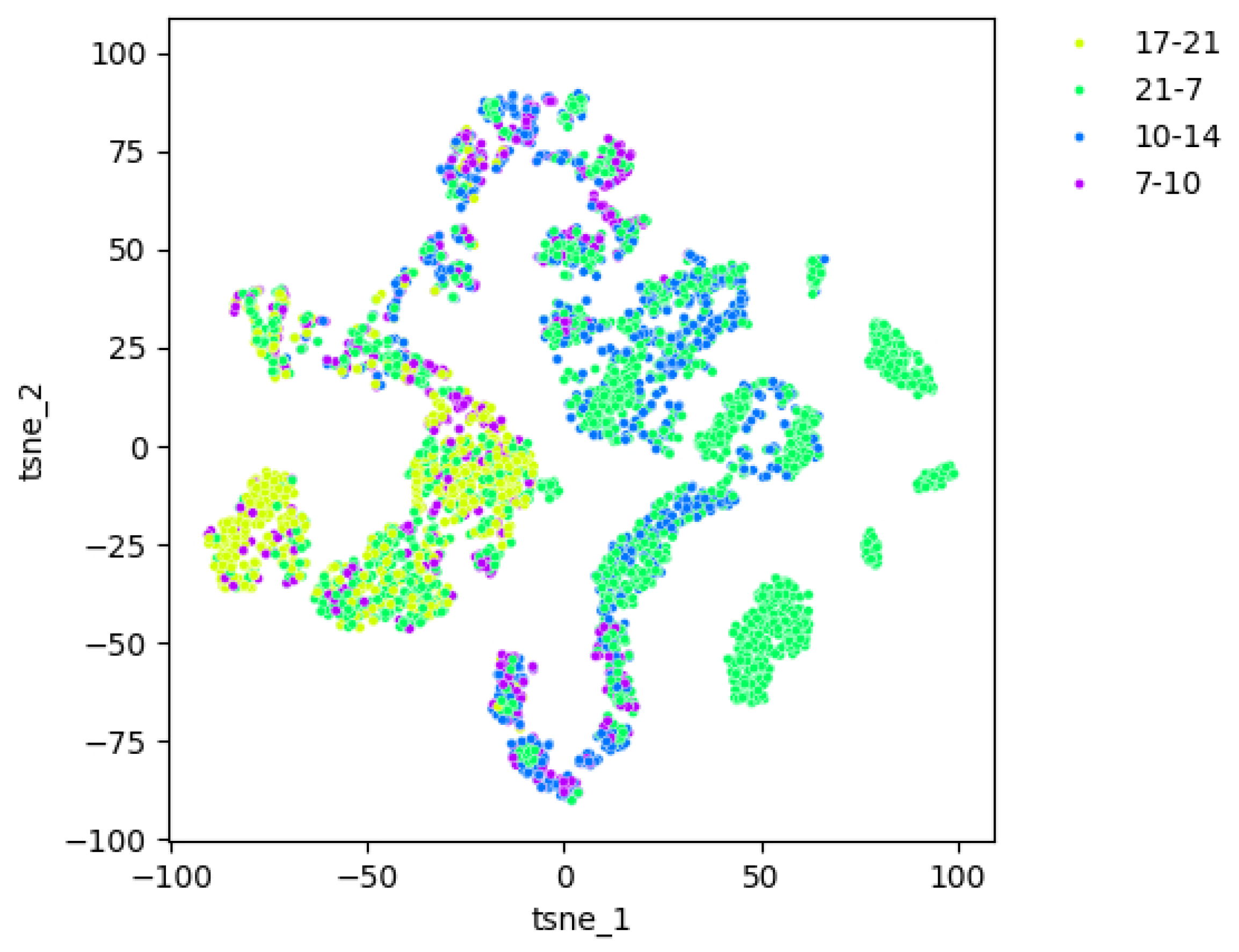
In addition, in order to visualize the sample data, this paper firstly generates four time period labels for the data according to the time period, and then uses the t-distributed random neighborhood embedding (t-SNE) algorithm for dimensionality reduction. The visualization result is shown in Figure 5. From the distribution in the figure, it can be observed that the points within the cluster of the same color are denser, reflecting the local similarity of the distribution network data within the same segment, and the points of different colors form relatively independent clusters, which can indicate that the distribution network data have obvious pattern differences at different times of the daily cycle. It can be obtained that the distribution network data shows a regular pattern of change with the daily cycle, and the STADGNN model can model this temporal dependence and capture the evolution of the distribution network posture over time.
The model performance was evaluated using the mean absolute error (MAE), mean absolute percentage error (MAPE), and root mean square error (RMSE). The smaller the values of the evaluation metrics e M A E , e M A P E , and e R M S E , the higher the prediction accuracy of the model, which is calculated as follows:
e M A E = i = 1 N Y i y i N
e M A P E = i = 1 N Y i y i y i N
e R M S E = i = 1 N Y i y i 2 N
where Y i represents the true value of the sample, y i represents the predicted value of the sample, and N represents the number of samples.

3.2. Parameter Details and Baseline Methods

In the experiments, the STADGNN model is implemented using the PyTorch 2.1.0 framework, and the mean absolute percentage error (MAPE) is selected as the loss function. In the experimental validation, all the experiments are set up to predict a sequence of situational values for the next 20 min (i.e., 4 points in the future) based on a sequence of historical 20 min runs. The detailed parameter settings of the STADGNN model are shown in Table 1, and the parameter settings for the other eight comparison algorithms are the same as the hyperparameter settings for STADGNN.
To further validate the performance of our proposed model, we conducted a comparative analysis of eight other baseline models under different conditions, including overall situation values, node voltage overturn margin index values, branch load severity index values, and node situation values.
(1)
CNN: convolutional neural network.
(2)
LSTM [4]: long short-term memory network, a special type of RNN model.
(3)
LSTMGC [9]: a hybrid model combining long short-term memory networks and graph convolutional networks.
(4)
EMA-SVD-Elman [7]: Elman neural network combined with the EMD-SVD method.
(5)
MSTGCN [9]: multi-component spatio-temporal graph convolutional network.
(6)
ASTGCN [9]: attention-based spatio-temporal graph convolutional network. Adds spatio-temporal attention to the MSTGCN.
(7)
LSTMA [5]: a long short-term memory network combined with an attention mechanism.
(8)
TPA-BiLSTM [6]: a model based on temporal pattern attention mechanisms and a bidirectional long short-term memory network.

3.3. Analysis of Experimental Results

3.3.1. Prediction Effectiveness Testing

To verify the accuracy of the STADGNN model proposed in this paper, the test set samples and the above eight prediction model methods are used under the same conditions to obtain the mean absolute error, root mean square error, and mean absolute percentage error between the output security situation prediction assessment value and the actual assessment value, as shown in Table 2. Additionally, under the same conditions, predictions are made for the node voltage overturn margin index values and branch load severity index values, resulting in comparison tables of prediction performance metrics for different models, as shown in Table 3 and Table 4. The best results are indicated in bold in the table, and underscores indicates the second best results. Through numerical analysis of the results in Table 2, it can be seen that, in terms of prediction evaluation values, the proposed STADGNN model reduced MAE, RMSE, and MPAE to 95.37%, 98.41%, and 94.69% of the original values, respectively, compared with the best-performing model, LSTMGC. Through numerical analysis of the results in Table 3, it can be seen that, in terms of the predicted node voltage overturn margin index values, the STADGNN model proposed in this paper reduced MAE, RMSE, and MPAE to 55.56%, 66.67%, and 62.37% of the original values, respectively, compared with the best-performing model, ASTGCN. Through numerical analysis of the results in Table 4, it can be seen that, in terms of the risk index value for predicting branch load severity values, the proposed STADGNN model reduced MAE, RMSE, and MPAE to 83.81%, 88.63%, and 65.78% of the original values, respectively, compared with the best-performing model, ASTGCN. Based on the comparison of performance metric parameters, it can be concluded that the STADGNN model achieves higher accuracy than other prediction models, and the proposed model outperforms all baseline methods.

3.3.2. Situation Indicators Testing

(1) Node voltage overturn margin
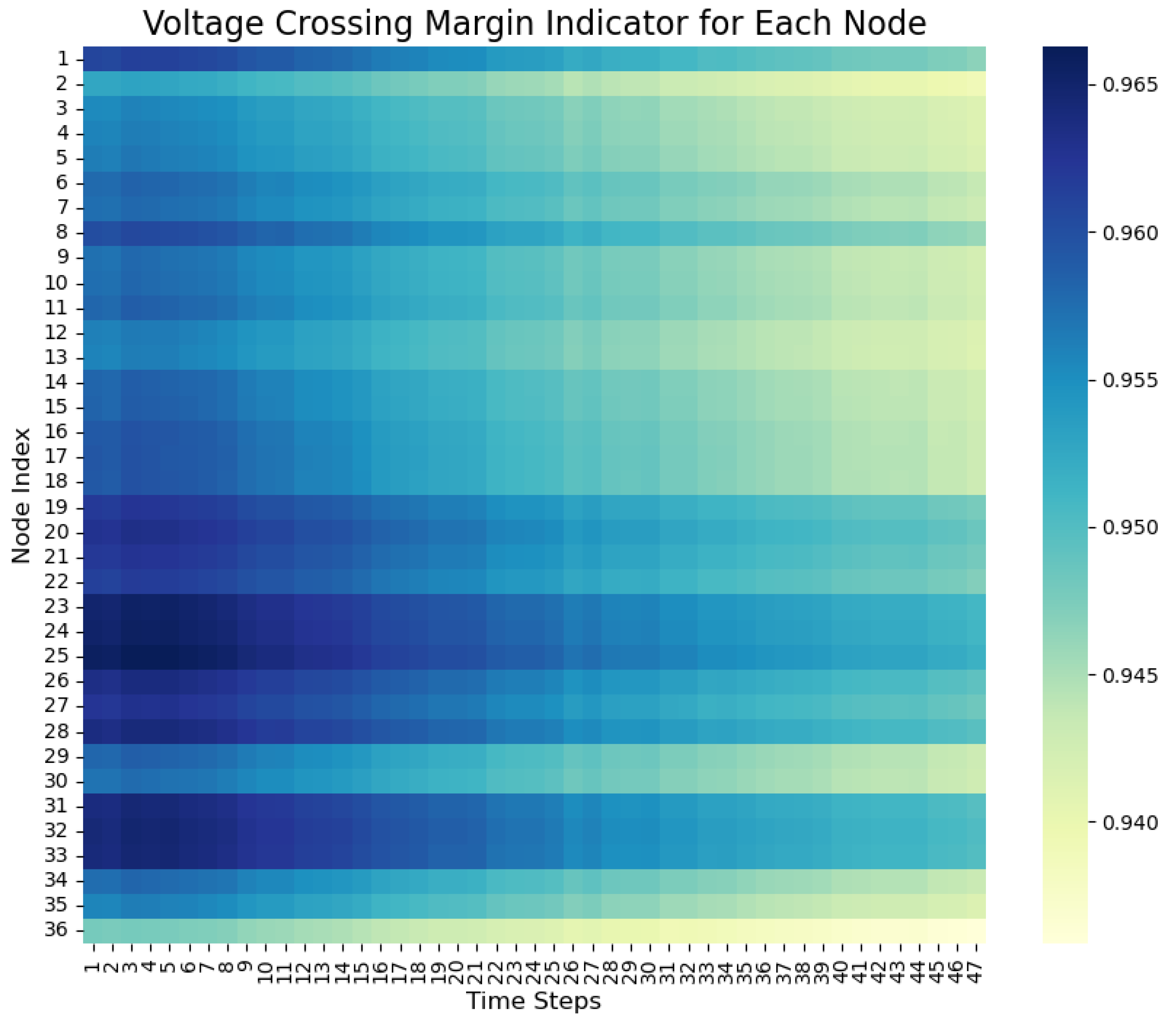
The voltage overturn conditions of each node are shown in Figure 6. It can be seen that most nodes are within the normal range of [0.95, 1.05], indicating being in a normal state. However, node 36 experiences low-voltage out-of-limit conditions due to insufficient load, falling within the range of [0.94, 0.95], thus requiring further voltage regulation. This indicator effectively reflects the severity of out-of-limit conditions of some nodes with small loads. As shown in Figure 7, the average absolute error of the voltage overturn risk index of each node is less than 0.06%, which is relatively accurate. Therefore, the proposed method can effectively perceive and predict the voltage state of the distribution network.
(2) Branch overload risk index
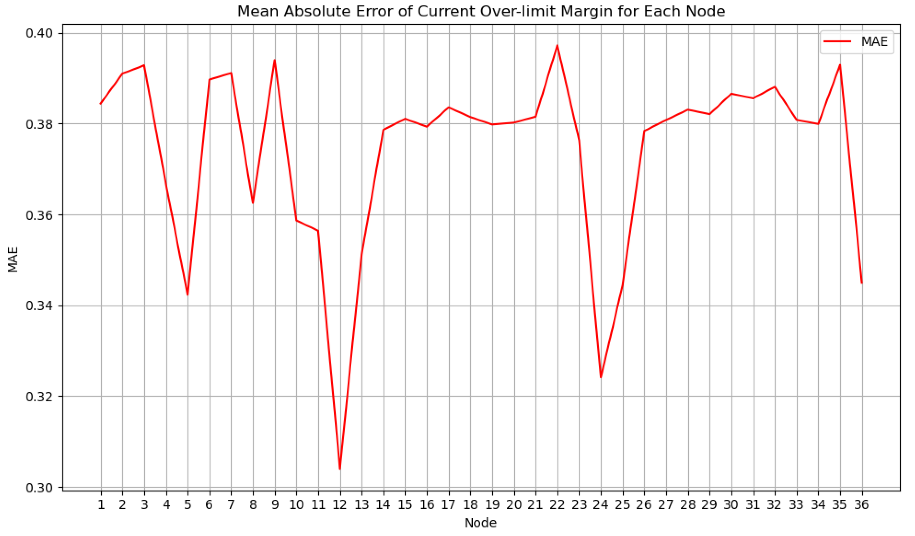
The overload risk index of each branch is shown in Figure 8. It can be seen that branch 6 is in a heavy load state and there is an operational risk. Most branches are in a normal operating state [0,0.4], but still need to be monitored at all times. As shown in Figure 9, the average absolute error of the overload risk index of each branch is less than 0.4, which is at a good level. Therefore, the proposed method can effectively perceive and predict the load status of the distribution network.

3.3.3. Node Assessment Values

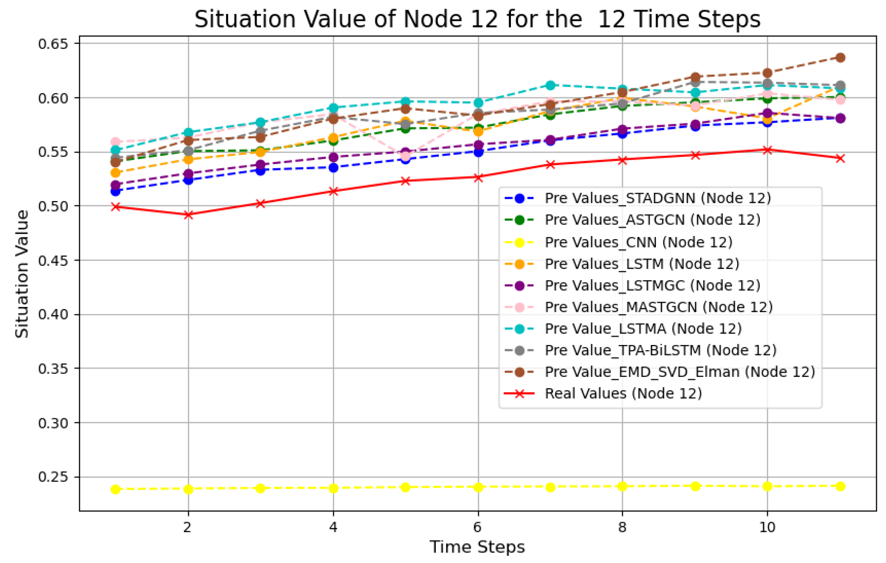
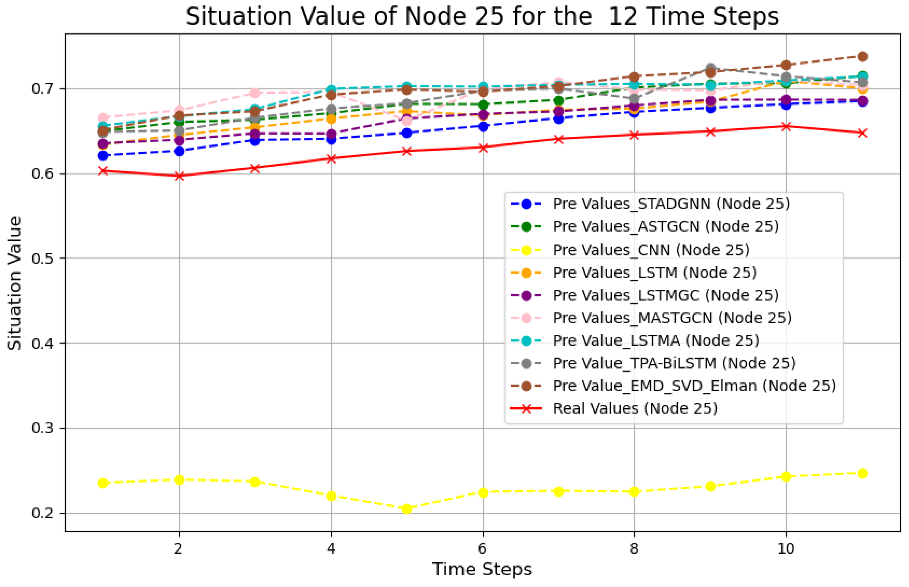
As shown in Figure 10, Figure 11 and Figure 12, the true values of the evaluation values for nodes 5, 12, and 25 at 12 time steps are compared with the predicted values of each model through visualization of the results. It can be seen that the proposed prediction model has high prediction accuracy for the evaluation values, and the predicted values are basically consistent with the true values. The prediction results of the CNN model in the figure (presented as horizontal lines) reflect the inherent limitations of the model when dealing with the task of time-series prediction. Unlike recurrent neural networks or attention-based models, standard CNNs lack explicit mechanisms to maintain and utilize long time-series information, and tend to learn “global average” behavior rather than temporal dynamic features when applied to time-series prediction, resulting in insufficient sensitivity to input variations. This phenomenon further validates the necessity of the STADGNN modeling of spatio-temporal dependencies in distribution network forecasting.

3.3.4. The Ablation Experiments

In order to further evaluate the effect of different components in the STADGNN, ablation experiments are conducted in this paper. Two different versions of STADGNN variants are designed in time and space dimensions, respectively. The details are as follows:
(1)
No Temporal Position Embedding–STADGNN (noTE-STADGNN): It removes the role of temporal position embedding to study the modeling of sequential information of sequences;
(2)
No Temporal Dynamic Perception–STADGNN (noTDP-STADGNN): It replaces a multi-head self-attention module with temporal dynamic perception with a conventional multi-head self-attention module to investigate the role of taking dynamic perception into account in prediction.
(3)
No Spatial Position Embedding–STADGNN (noSE-STADGNN): It removes spatial position embedding to investigate the role of modeling the inherent static spatial features of distribution networks;
(4)
No Spatial Dynamic Correlation Matrix–STADGNN (noSDCM-STADGNN): It removes the spatial dynamic correlation matrix in order to study the role of dynamically adjusting the strength of the spatial correlation instead of basing it solely on static topological relations.
Except for the differences mentioned above, all four STADGNN variant models have the same setup as the STADGNN. The results of the predictive performance metrics of these models are given in Table 5. We can observe that temporal position embedding is an important component in the time dimension by comparing the noTE-STADGNN and STADGNN. The noTE-STADGNN operates without position embedding and sequential information, and performs worse than the STADGNN. In addition, the STADGNN outperforms the noTDP-STADGNN, a result that demonstrates the effectiveness of modeling using multi-head self-attention with temporal dynamics awareness. In the spatial dimension, both the noSE-STADGNN model and the noSDCM-STADGNN model perform worse than yjr STADGNN, which suggests that the consideration of static spatial features can help to capture spatial location and attribute differences in distribution network data, and also demonstrates that it is important to dynamically adjust the strength of spatial correlations in the STADGNN. The superiority of the STADGNN model is further verified by ablation experiments.

4. Conclusions

In this paper, we propose a distribution network situational awareness prediction method based on an STADGNN model. Through spatio-temporal dynamic correlation modeling and the introduction of a spatio-temporal position embedding module, a situation awareness prediction model adapted to the complex characteristics of distribution networks is constructed, providing a new method for solving the problems of insufficient spatio-temporal correlation mining and the insufficient adaptability of dynamic topological structures in traditional methods. The STADGNN proposed in this paper outperforms eight baseline models in all three assessment metrics (MAE, RMSE, MAPE) after averaging multiple repetitive experiments in different prediction tasks of integrated assessment values, voltage overturn margin index values, and branch load severity index values using simulation data from the IEEE37 bus test system, and these results confirm that the STADGNN is able to accurately capture the temporal and spatial dynamics and adapt to topology changes, providing reliable support for distribution network security situation prediction. The ablation experiments further confirmed the need for key components of the STADGNN model.
However, the proposed STADGNN approach still has some limitations that need to be addressed. Firstly, the current validation relies on simulation data from the IEEE37 bus test system, and its performance in real distribution networks remains to be verified. Secondly, for second-level data, the model still needs to be strengthened to handle sudden changes in physical topology at the second level. To address these limitations and expand the applicability of the methodology, future work will focus on the directions of applying the model to real distribution network measurement data, enhancing the dynamic topology processing capability.

Author Contributions

Conceptualization, X.Q., Y.H. and G.L.; methodology, X.Q. and G.L.; software, X.Q.; validation, X.Q., G.L. and J.Y.; formal analysis, X.Q., G.L. and S.C.; investigation, X.Q., G.L. and Y.H.; resources, X.Q., G.L. and J.Y.; data curation, X.Q. and S.C.; writing—original draft preparation, X.Q.; writing—review and editing, X.Q. and G.L.; visualization, X.Q.; supervision, X.Q. and G.L.; project administration, X.Q., G.L. and Y.H. All authors have read and agreed to the published version of the manuscript.

Funding

This research was partly funded by State Grid Zhejiang Electric Power Co., Ltd. technology project (B311XT24004V).

Data Availability Statement

The original contributions presented in this study are included in the article. Further inquiries can be directed to the corresponding author.

Conflicts of Interest

Authors Yuteng Huang, Jiaxiang Yan and Shan Chen were employed by the company State Grid Zhejiang Electric Power Co., LTD. The remaining authors declare that the research was conducted in the absence of any commercial or financial relationships that could be construed as a potential conflict of interest.

References

  1. Sonal; Ghosh, D. Impact of situational awareness attributes for resilience assessment of active distribution networks using hybrid dynamic Bayesian multi criteria decision-making approach. Reliab. Eng. Syst. Saf. 2022, 228, 108772. [Google Scholar] [CrossRef]
  2. Ge, L.J.; Li, Y.L.; Li, Y.L.; Yan, J.; Sun, Y.H. Smart Distribution Network Situation Awareness for High-Quality Operation and Maintenance: A Brief Review. Energies 2022, 15, 828. [Google Scholar] [CrossRef]
  3. Fang, Z.; Lin, Y.; Song, S.; Li, C.; Lin, X.; Chen, Y. State Estimation for Situational Awareness of Active Distribution System With Photovoltaic Power Plants. IEEE Trans. Smart Grid 2021, 12, 239–250. [Google Scholar] [CrossRef]
  4. Tian, S.X.; Li, K.P.; Wei, S.R.; Fu, Y.; Li, Z.K.; Liu, S. Security Situation Awareness Approach for Distribution Network Based onSynchronous Phasor Measurement Unit. Proc. CSEE 2021, 41, 617–632. (In Chinese) [Google Scholar] [CrossRef]
  5. Xie, Z.J.; Zhang, D.X.; Han, X.Q.; Hu, W. Research on Transient Stability Assessment Method of Power System Based on Improved Long Short Term Memory Network. Power Syst. Technol. 2024, 48, 998–1010. (In Chinese) [Google Scholar] [CrossRef]
  6. Xu, F.Q.; Li, Q.S.; Song, L.; Zheng, Z.X.; Chen, X.; Hu, Q. Situation Awareness of Distribution Network Based on TPA-BiLSTM. In Proceedings of the 2024 7th International Conference on Renewable Energy and Power Engineering (REPE), Beijing, China, 25–27 September 2024; pp. 80–84. [Google Scholar] [CrossRef]
  7. Luo, Y.H.; Cheng, Q.; Yan, S.J.; Yang, D.S. Situation awareness method of the distribution network based on EMD-SVD and Elman neural network. Energy Rep. 2022, 8, 632–639. [Google Scholar] [CrossRef]
  8. Huang, M.Y.; Guo, J.W.; Zang, H.X.; Fang, X.C.; Wei, Z.N.; Sun, G.Q. State Estimation of Power System Based on a Message Passing Neural Network. Power Syst. Technol. 2023, 47, 4396–4409. (In Chinese) [Google Scholar] [CrossRef]
  9. Guo, S.N.; Lin, Y.F.; Feng, N.; Song, C.; Wan, H.Y. Attention Based Spatial-Temporal Graph Convolutional Networks for Traffic Flow Forecasting. Proc. AAAI Conf. Artif. Intell. 2019, 33, 922–929. [Google Scholar] [CrossRef]
  10. Khodayar, M.; Wang, J. Spatio-Temporal Graph Deep Neural Network for Short-Term Wind Speed Forecasting. IEEE Trans. Sustain. Energy 2019, 10, 670–681. [Google Scholar] [CrossRef]
  11. Simeunović, J.; Schubnel, B.; Alet, P.J.; Carrillo, R.E.; Frossard, P. Interpretable temporal-spatial graph attention network for multi-site PV power forecasting. Appl. Energy 2022, 327, 120127. [Google Scholar] [CrossRef]
  12. Li, Z.; Ye, L.; Zhao, Y.; Pei, M.; Lu, P.; Li, Y.; Dai, B. A Spatiotemporal Directed Graph Convolution Network for Ultra-Short-Term Wind Power Prediction. IEEE Trans. Sustain. Energy 2023, 14, 39–54. [Google Scholar] [CrossRef]
  13. Zhang, J.; Hu, X.; Ren, C.; Zhan, Z.; Wang, T.; Ma, D. Short-Term Load Forecasting Based on Spatial-Temporal Correlation for Virtual Power Plant. In Proceedings of the 2024 3rd International Conference on Power Systems and Electrical Technology (PSET), Tokyo, Japan, 5–8 August 2024; pp. 791–796. [Google Scholar] [CrossRef]
  14. Jiang, H.; Dong, Y.; Dong, Y.; Wang, J. Power load forecasting based on spatial–temporal fusion graph convolution network. Technol. Forecast. Soc. Change 2024, 204, 123435. [Google Scholar] [CrossRef]
  15. Vaswani, A.; Shazeer, N.; Parmar, N.; Uszkoreit, J.; Jones, L.; Gomez, A.N.; Kaiser, Ł.; Polosukhin, I. Attention is all you need. Adv. Neural Inf. Process. Syst. 2017, 30, 5998–6008. [Google Scholar]
  16. Sutskever, I.; Vinyals, O.; Le, Q.V. Sequence to sequence learning with neural networks. In Proceedings of the 28th International Conference on Neural Information Processing Systems—Volume 2 (NIPS’14), Montreal, QC, Canada, 8–13 December 2014; pp. 3104–3112. [Google Scholar]
  17. He, K.M.; Zhang, X.Y.; Ren, S.Q.; Sun, J. Deep Residual Learning for Image Recognition. In Proceedings of the 2016 IEEE Conference on Computer Vision and Pattern Recognition (CVPR), Las Vegas, NV, USA, 27–30 June 2016; pp. 770–778. [Google Scholar] [CrossRef]
  18. Ba, J.L.; Kiros, J.R.; Hinton, G.E. Layer normalization. arXiv 2016, arXiv:1607.06450. [Google Scholar] [CrossRef]
  19. Li, S.; Jin, X.; Xuan, Y.; Zhou, X.; Chen, W.; Wang, Y.X.; Yan, X. Enhancing the Locality and Breaking the Memory Bottleneck of Transformer on Time Series Forecasting. In Proceedings of the Advances in Neural Information Processing Systems 33, Volume 7 of 20: 33rd Conference on Neural Information Processing Systems (NeurIPS 2019), Vancouver, BC, Canada, 8–14 December 2019. [Google Scholar]
  20. Kipf, T.N.; Welling, M. Semi-Supervised Classification with Graph Convolutional Networks. arXiv 2016, arXiv:1609.02907. [Google Scholar]
  21. Guo, S.N.; Lin, Y.F.; Wan, H.Y.; Li, X.C.; Cong, G. Learning dynamics and heterogeneity of spatial-temporal graph data for traffic forecasting. IEEE Trans. Knowl. Data Eng. 2021, 34, 5415–5428. [Google Scholar] [CrossRef]
  22. Li, Q.M.; Han, Z.C.; Wu, X.M. Deeper insights into graph convolutional networks for semi-supervised learning. Proc. AAAI Conf. Artif. Intell. 2018, 32. [Google Scholar] [CrossRef]
  23. Zhao, H.; Zhang, H.; Ge, Y.; Gao, W.; Li, J.; Su, B.; Cheng, K. Reliability Evaluation of Distribution Network Based on Situation Awareness. In Proceedings of the 2019 IEEE Sustainable Power and Energy Conference (iSPEC), Beijing, China, 21–23 November 2019; pp. 2043–2048. [Google Scholar] [CrossRef]
  24. Ge, L.; Li, Y.; Li, S.; Zhu, J.; Yan, J. Evaluation of the situational awareness effects for smart distribution networks under the novel design of indicator framework and hybrid weighting method. Front. Energy 2021, 15, 143–158. [Google Scholar] [CrossRef]
  25. Lin, Y.F.; Wang, X.Y. A Data-Driven Scheme Based on Sparse Projection Oblique Randomer Forests for Real-Time Dynamic Security Assessment. IEEE Access 2022, 10, 79469–79479. [Google Scholar] [CrossRef]
  26. Yang, H.Y.; Zeng, R.Y.; Xu, G.Q.; Zhang, L. A network security situation assessment method based on adversarial deep learning. Appl. Soft Comput. 2021, 102, 107096. [Google Scholar] [CrossRef]
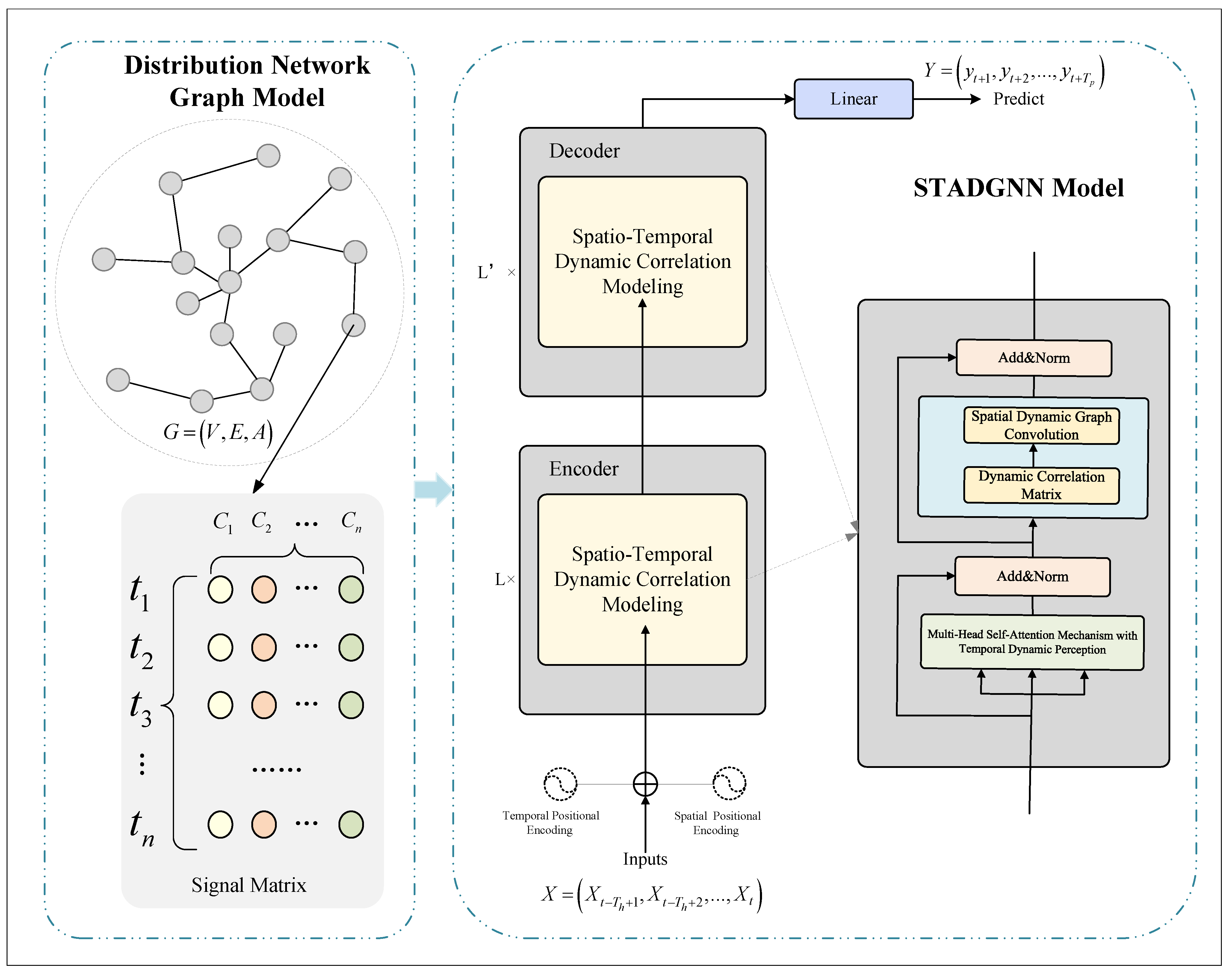
Figure 1. Components of the security situational awareness system model. It contains the distribution network graph model and the STADGNN model.
Energies 18 04402 g001
Figure 2. The architecture of the STADGNN model. It adopts an encoder–decoder structure and contains spatio-temporal dynamic correlation modeling modules that contain the multi-head self-attention mechanism with temporal dynamic perception, the spatial dynamic graph convolution module, and the dynamic correlation matrix.
Energies 18 04402 g002
Figure 3. Flow chart of situational awareness realization.
Energies 18 04402 g003
Figure 4. The topology of the IEEE37 bus test system.
Energies 18 04402 g004
Figure 5. Visualization of t-distributed random neighborhood embedding (t-SNE) of data.
Energies 18 04402 g005
Figure 6. Voltage overrun risk degree indicator for each node.
Energies 18 04402 g006
Figure 7. Mean absolute error of the voltage overrun riskiness index at each node.
Energies 18 04402 g007
Figure 8. Current overload risk degree indicator for each branch circuit.
Energies 18 04402 g008
Figure 9. Mean absolute error of the current overload riskiness index for each branch.
Energies 18 04402 g009
Figure 10. Comparison of node 5 assessment projections among different methods.
Energies 18 04402 g010
Figure 11. Comparison of node 12 assessment projections among different methods.
Energies 18 04402 g011
Figure 12. Comparison of node 25 assessment projections among different methods.
Energies 18 04402 g012
Table 1. The detailed parameter settings of the STADGNN model.
ParametersValue
Model dimension ( d model )64
Number of attention heads (h)8
Learning rate ( l r )0.001
Number of encoder layers (L)3
Number of decoder layers ( L )3
Size of the convolution kernel (k)3
Epochs100
Batch size32
Dropout rate ( D r )0.005
Table 2. Comparison of the performance of different models in predicting assessment values.
ModelMAERMSEMAPE
STADGNN0.01030.02473.4222
ASTGCN0.01080.02493.6874
CNN0.01180.02584.0773
LSTM0.01790.03336.5887
LSTMGC0.01080.02513.6142
MSTGCN0.01650.03285.9383
LSTMA0.01460.02895.2442
TPA-BiLSTM0.01470.02935.2771
EMD-SVD-Elman0.01580.031336.6274
Table 3. Performance comparison of voltage overlimit risk index values predicted by different models.
ModelMAERMSEMAPE
STADGNN0.00050.00080.0557
ASTGCN0.00090.00120.0893
CNN0.00140.00410.1442
LSTM0.00160.00240.1687
LSTMGC0.00190.00330.2002
MSTGCN0.00150.00240.1591
LSTMA0.00160.00240.1615
TPA-BiLSTM0.00150.00230.1573
EMD-SVD-Elman0.00150.00220.1591
Table 4. Performance comparison of risk index values for branch overload predictions using different models.
ModelMAERMSEMAPE
STADGNN0.23040.29937.3780
ASTGCN0.27490.337711.3796
CNN0.46071.335211.2167
LSTM0.33490.401018.3343
LSTMGC0.28910.356111.6696
MSTGCN0.31850.388717.2258
LSTMA0.32410.393217.5371
TPA-BiLSTM0.31720.381017.1222
EMD-SVD-Elman0.32150.379417.8959
Table 5. Comparison of ablation experiment results.
ModelMAERMSEMAPE
STADGNN0.01030.02473.4222
noTE-STADGNN0.01080.02523.6620
noTDP-STADGNN0.01060.02523.5305
noSE-STADGNN0.01060.02513.5152
noSDCM-STADGNN0.01050.02473.5181
Disclaimer/Publisher’s Note: The statements, opinions and data contained in all publications are solely those of the individual author(s) and contributor(s) and not of MDPI and/or the editor(s). MDPI and/or the editor(s) disclaim responsibility for any injury to people or property resulting from any ideas, methods, instructions or products referred to in the content.