Article

Gramian Angular Field–Gramian Adversial Network–ResNet34: High-Accuracy Fault Diagnosis for Transformer Windings with Limited Samples

1
Electric Power Research Institute of Yunnan Power Grid, Kunming 650214, China
2
School of Electrical Engineering, Southwest Jiaotong University, Chengdu 611756, China
*
Author to whom correspondence should be addressed.
Energies 2025, 18(16), 4329; https://doi.org/10.3390/en18164329
Submission received: 24 June 2025 / Revised: 9 August 2025 / Accepted: 11 August 2025 / Published: 14 August 2025

Abstract

Transformers are critical equipment in power transmission and distribution systems, and the condition of their windings significantly impacts their reliable operation. Therefore, the fault diagnosis of transformer windings is of great importance. Addressing the challenge of limited fault samples in traditional diagnostic methods, this study proposes a small-sample fault diagnosis method for transformer windings. This method combines data augmentation using the Gramian angular field (GAF) and generative adversarial networks (GAN) with a deep residual network (ResNet). First, by establishing a transformer winding fault simulation experiment platform, frequency response curves for three types of faults—axial displacement, bulging and warping, and cake-to-cake short circuits—and different fault regions were obtained using the frequency response analysis method (FRA). Second, a frequency response curve image conversion technique based on the Gramian angular field was proposed, converting the frequency response curves into Gramian angular summation field (GASF) and Gramian angular difference field (GADF) images using the Gramian angular field. Next, we introduce several improved GANs to augment the frequency response data and evaluate the quality of the generated samples. We compared and analysed the diagnostic accuracy of ResNet34 networks trained using different GAF–GAN combination datasets for winding fault types, and we proposed a transformer winding small-sample fault diagnosis method based on GAF-GAN-ResNet34, which can achieve a fault identification accuracy rate of 96.88% even when using only 28 real samples. Finally, we applied the proposed fault diagnosis method to on-site transformers to verify its classification performance under small-sample conditions. The results show that, even with insufficient fault samples, the proposed method can achieve high diagnostic accuracy.

1. Introduction

As a core device in power systems, the operating status of transformers directly affects the safety and stability of power systems [1,2]. Winding faults are the main type of transformer faults. During operation, transformer windings are susceptible to short-circuit current impacts. Under the cumulative effect of electrodynamic forces, they are prone to deformation faults such as displacement and buckling, which severely affect the reliability of transformer operation [3]. Therefore, accurate diagnosis of the status of transformer windings is of great significance.
Currently, the main methods for detecting faults in transformer windings include the short-circuit impedance method, frequency response method, and vibration method. Among these, the frequency response method is widely adopted due to its strong anti-interference capability, high testing sensitivity, and intuitive result analysis [4]. In recent years, with the continuous improvement of computer hardware performance and the iterative optimisation of deep learning algorithms, the application of intelligent diagnostic methods in transformer winding frequency response analysis has garnered significant attention. Neural networks can extract features from large datasets and iteratively optimise model parameters to efficiently solve complex problems, making them an extremely suitable intelligent algorithm for frequency response data analysis. Reference [5] utilised an artificial neural network (ANN) to identify common winding faults; reference [6] used the change in the frequency response curve between zero and pole points as input features for the artificial neural network, achieving good diagnostic results; however, the process of constructing such a network is relatively complex and requires further simplification; reference [7] proposed using a backpropagation (BP) neural network to determine the type of winding fault, selecting the correlation coefficient and standard deviation as feature inputs. However, during actual training, it was found that the convergence speed of this network was slow, resulting in a longer training time. Reference [8] recognised the limitations of the BP neural network and improved its structure, eliminating directional detection errors while enhancing the accuracy of the BP neural network in detecting winding faults. Reference [9] used the binary image reconstructed from the frequency response curve as input, using a convolutional neural network (CNN) to identify winding faults, achieving a recognition accuracy of 95% on the test set, demonstrating excellent diagnostic performance; reference [10] optimised the CNN structure using bidirectional gated recurrent unit (BiGRU), further enhancing the CNN’s ability to distinguish winding faults. As demonstrated by the above research, compared to other intelligent diagnostic algorithms, the CNN achieves higher accuracy in winding fault diagnosis tasks. This is because the CNN can utilise convolutional layers to extract local features from the data while reducing computational load and parameter complexity through pooling layers, thereby demonstrating robust classification and recognition capabilities.
However, transformer equipment has high reliability, and winding faults are rare events. This results in a scarcity of winding fault samples available to scholars and researchers in actual transformer operation sites, with significant variations in the number of samples across different fault types. Despite its many advantages, FRA faces two key challenges: sample scarcity, with fewer than five critical fault features per utility company per year; and interpretability gaps, with uncertainty in the physical-to-feature mapping in AI models. To address these issues, reference [11] proposed a transformer winding deformation fault identification method based on a twin convolutional network to attempt to resolve the problem of imbalanced fault data; reference [12] proposes a data-mechanism-driven method that fuses virtual and real features, introducing a transformer simulation model to compensate for the lack of actual sample features, and improves the average identification accuracy by 27.1% in a small-sample scenario with 30% data; reference [13] uses Conditional-WGAN-GP to augment small-batch fault winding FRC data, and applied the expanded data to the training of an SVM classification network to obtain a fault diagnosis model. Diagnostic results indicate that GAN data expansion can significantly improve fault identification accuracy. A comparison of existing major transformer fault analysis and diagnosis methods is shown in Table 1. However, current research on transformer winding fault diagnosis in small-sample scenarios remains inadequate, with limited research content and scarce outcomes. It urgently requires more attention and exploration from scholars and researchers to drive progress and development in this field. This study addresses these issues by combining GAF visualization with GAN-based few-shot learning [3,14,15,16].
To this end, this paper has conducted the following work on transformer winding fault diagnosis: First, by establishing a transformer winding fault simulation experiment platform, the frequency response method was used to obtain frequency response curves for different fault types and fault regions of the windings, providing data support for subsequent intelligent diagnosis; second, a GAF image conversion technique was proposed, using GAF to convert the frequency response curves into GADF and GASF images; then, we introduced multiple improved GANs to augment the frequency response data and evaluated the quality of the generated samples. A comparative analysis was conducted on the diagnostic accuracy of winding fault types using different GAF–GAN combined datasets to train the ResNet34 network, proposing a transformer winding fault diagnosis method based on GAF–GAN–ResNet34 for small-sample scenarios. Finally, the proposed fault diagnosis method is applied to field transformers to verify its classification performance under small-sample conditions.

2. Obtaining the Winding Frequency Response Curve

2.1. Basic Principles of FRA

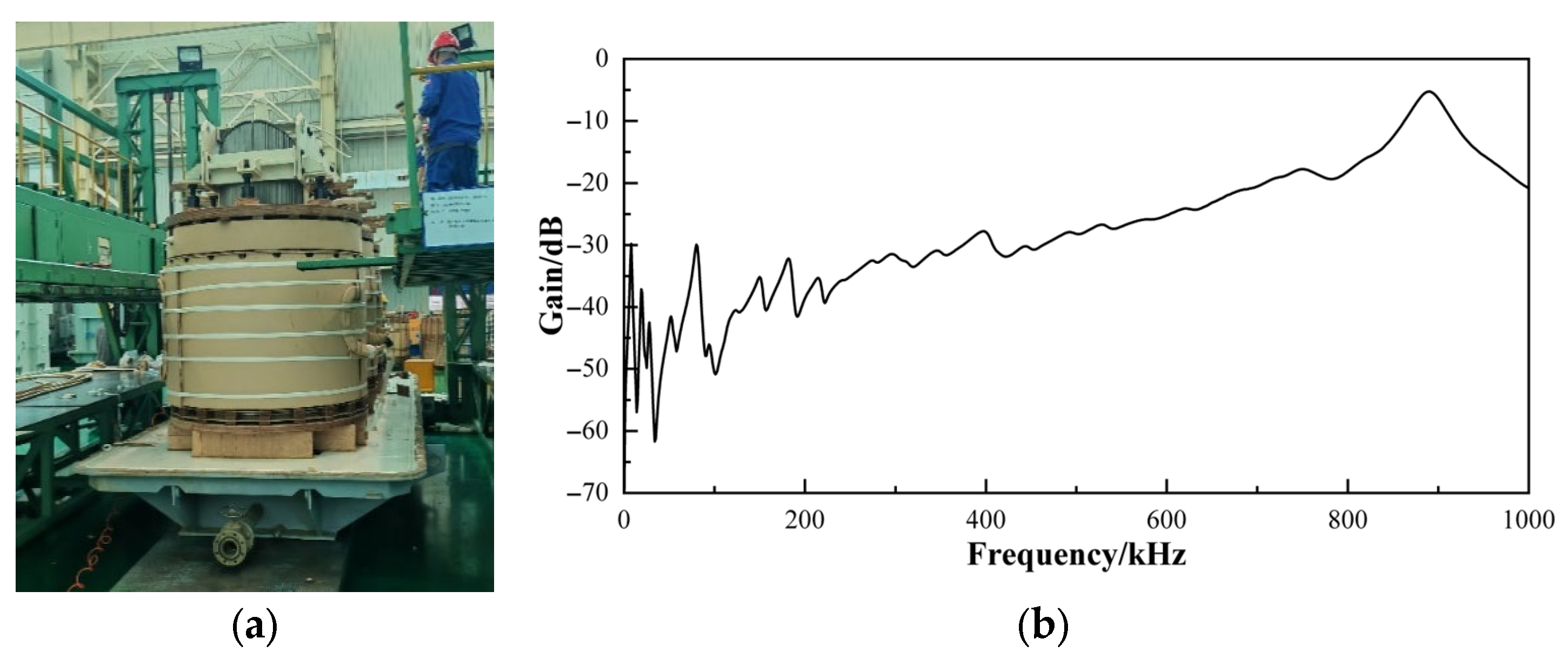
Under the influence of high-frequency excitation, the transformer winding can be regarded as a passive two-port network composed of distributed parameters such as linear resistance, inductance, and capacitance. The parameters of this network are uniquely determined by the geometric structure of the transformer [17]. Sine excitation signals of different frequencies (1~1000 kHz) are injected into the input terminals of the transformer windings, and the corresponding response signals are measured at the output terminals. By calculating the ratio of the response signals to the excitation signals at different frequencies, the frequency response curves are obtained.
H ( f ) = 20 lg U o u t ( f ) U i n ( f ) φ ( f ) = φ ( U o u t ( f ) ) φ ( U i n ( f ) )
where H(f) and φ(f) are the amplitude and phase of the frequency response; Uout(f) and Uin(f) are the terminal voltage and excitation voltage of the winding response, respectively; f is the frequency of the applied signal.
When a transformer winding fails, the equivalent parameters (such as capacitance and inductance) in its equivalent two-port network change compared to its healthy state, resulting in changes to its frequency response. For different types of winding faults, the patterns of change in the equivalent two-port network vary, resulting in different patterns of change in FRA results compared to those under healthy conditions. However, for the same type of fault, even if the specific location and severity of the fault differ, the changes in electrical parameters and FRA results still exhibit a certain degree of similarity. Therefore, by analysing the patterns of change in the FRA results of the windings, the type of transformer winding fault can be determined.

2.2. Test Platform Construction

Winding fault simulations on operational transformers are rarely performed due to the destructive nature of tests and high equipment costs. To address this limitation, we established a dedicated fault simulation platform using a 10 kV test transformer, as shown in Figure 1a. The FRA is conducted through the high-voltage (HV) winding, as shown in Figure 1b. The structural parameters of the test transformer are shown in Table 2. The transformer windings are structured as coil segments, with copper terminals welded at both ends of each segment. The segments are connected using high-conductivity brass nuts. The segments are numbered from 1 to 16 from top to bottom, and the interconnections between segments are numbered from 1 to 15 from top to bottom.
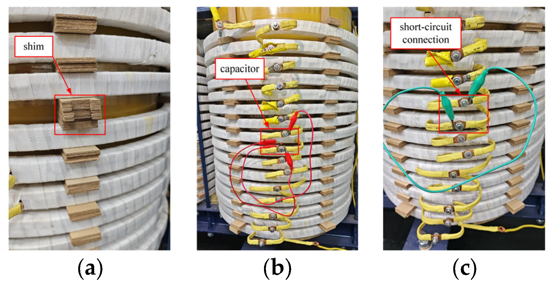
In order to obtain frequency response curves for different types of winding faults, fault locations, and fault severities, three types of transformer faults were simulated based on the frequency response test platform: axial displacement fault (AD), bulging and warping fault (SCV), and cake-to-cake short circuit fault (SC). The simulations of each type of fault are shown in Figure 2.
(1)
AD
AD refers to a fault in which the windings of a transformer shift along the transformer’s axis during operation due to the effects of electromagnetic or mechanical forces. In this paper, ADs are simulated by increasing the number of spacers under the windings, as shown in Figure 2a. Depending on the fault location and severity, four types of AD were set up, as shown in Table 3. The severity of the fault is defined as the ratio of the AD distance of the windings to the height of the coil.
(2)
SCV
SCV refers to a fault in which a portion of the transformer winding undergoes local deformation or bulging due to factors such as uneven stress, thermal stress, or manufacturing defects. When SCV occurs, the equivalent capacitance of the winding along its longitudinal axis increases [18]. Therefore, this study simulates the bulging and warping fault by paralleling capacitors at the winding terminals, as shown in Figure 2b. Depending on the fault location and the value of the parallel capacitors, four different SCV scenarios were set up, as shown in Table 4.
(3)
SC
SC refers to a fault where the insulation layer between adjacent windings of a transformer is penetrated or damaged, resulting in an electrical short circuit between the windings. In this paper, SC is simulated by short-circuiting the terminal ports on the outer side of the windings, as shown in Figure 2c. Depending on the location of the fault, four types of SC were set up, as shown in Table 5.

2.3. Frequency Response Curve Data Acquisition and Analysis

Following the above experimental procedures, FRA were conducted on transformer windings under three typical fault conditions and under normal conditions. The test results are shown in Figure 3. For each type of fault, 28 sets of frequency response data were collected, with 7 sets of data collected for each specific fault condition. As a control, 28 sets of frequency response data were collected for transformer windings under normal conditions.
As shown in Figure 3a, when the winding experiences AD, the trough near 270 kHz shifts upward, the peak near 600 kHz shifts downward, the peak near 730 kHz shifts to the right, the trough near 800 kHz shifts upward and to the right, and the overall curve in the 500~700 kHz frequency band shifts downward, while the overall curve in the 800~1000 kHz frequency band shifts upward. The frequency response curve exhibits a certain degree of discrimination between different fault severities, but there is still some overlap between them.
As shown in Figure 3b, when the winding experiences SCV, the peak near 420 kHz shifts downward to the left when the parallel capacitance of the winding is 200 pF and shifts upward to the left when the parallel capacitance is 560 pF. The peak near 730 kHz shifts downward to the left when the parallel capacitance is 200 pF, shifts downward to the left when the parallel capacitance is 200 pF, and shifts downward to the right when the parallel capacitance is 560 pF. Additionally, a distinct resonance point appears in the 600~1000 kHz frequency band. This indicates that by analysing the shift in amplitude at the resonance points near 420~730 kHz, one can preliminarily determine the type of fault that has occurred.
As shown in Figure 3c, when SC occurs between the windings, the wave peak near 430 kHz shifts to the lower right. When a fault occurs in the middle of the winding, a distinct resonance point appears in the 400~600 kHz frequency band. When a fault occurs in the lower part of the winding, a distinct resonance point appears in the 800~900 kHz frequency band. The presence of new resonance points in the 400~600 kHz frequency band and the 800~900 kHz frequency band can be used to preliminarily determine the location of the fault.
The distinct impacts of AS, SC, and SCV on frequency response curves arise from their unique modifications to the winding’s equivalent electrical parameters. AD primarily alters longitudinal capacitance and mutual inductance, manifesting as a downward shift in mid-frequency resonance. SC reduce inter-turn impedance, causing global upward shifts and high-frequency noise. SCV increase localized capacitance, leading to amplitude elevation and resonance damping.
In summary, there is overlap between the frequency response curves under normal conditions and the three fault conditions, making it difficult to clearly identify the characteristic information on the curves. Further processing of the frequency response curves is required to accurately identify winding faults. Although composite faults were not physically simulated, their FR characteristics can be approximated as superpositions of single-fault signatures. This will be leveraged in virtual experiments.

3. Visualisation and Analysis of Frequency Response Data Based on GAF

GAF is an encoding method that combines coordinate transformation and Gram matrices to convert one-dimensional data into two-dimensional feature images. Depending on the transformation formula used, GAF is divided into two forms: GASF and GADF. GASF generates a Gram matrix by summing the angles between each data point and all other data points in the one-dimensional data; GADF calculates the angular differences between data points to construct the Gram matrix. GASF emphasises relative changes between data points, highlighting local dynamic characteristics of the data; GADF preserves the overall correlation between data points, making it more suitable for capturing and identifying global features of the data [19].

3.1. GAF Image Conversion Principle

The data processing method based on GAF is as follows:
(1)
Data normalisation: To ensure that the data are −1~1, normalise the data as shown in Equation (2).
x ˜ i = x i min ( X ) max ( X ) min ( X ) × 2 1
where X = {x1, x2, , xN} is the original data, and x ˜ i is the normalised value.
(2)
Calculate angle encoding: Map the normalised one-dimensional data to the angle in the polar coordinate system. The value of each data point is converted to the angle in the polar coordinate system, as shown in Equation (3):
ϕ i = arccos ( x ˜ i ) , x ˜ i [ 1 , 1 ]
(3)
Calculate the GAF matrix: Based on the angle information, calculate the GASF and GADF values as shown in Equations (4) and (5):
G A S F = cos ( φ 1 + φ 1 ) cos ( φ 1 + φ 2 ) cos ( φ 1 + φ n ) cos ( φ 2 + φ 1 ) cos ( φ 2 + φ 2 ) cos ( φ 2 + φ n ) cos ( φ n + φ 1 ) cos ( φ n + φ 2 ) cos ( φ n + φ n )
G A D F = cos ( φ 1 φ 1 ) cos ( φ 1 φ 2 ) cos ( φ 1 φ n ) cos ( φ 2 φ 1 ) cos ( φ 2 φ 2 ) cos ( φ 2 φ n ) cos ( φ n φ 1 ) cos ( φ n φ 2 ) cos ( φ n φ n )
(4)
Generate image: Generate GAF images based on the calculation results of GASF and GADF.

3.2. Steps for Converting GAF Images of Winding Frequency Response Curves

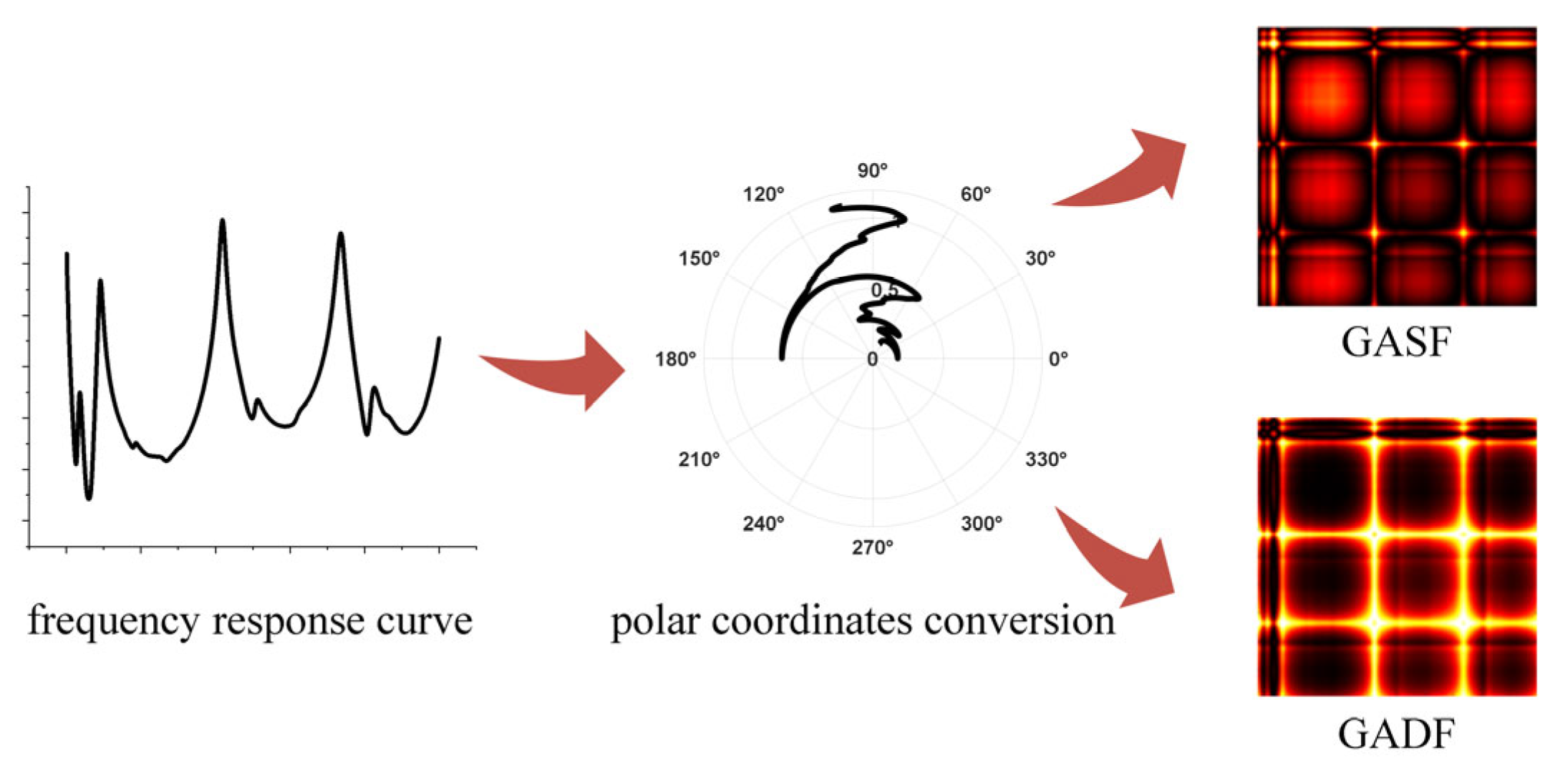
The Gram angle field image conversion method is based on transformer winding frequency response curves, as shown in Figure 4, with the specific steps as follows:
(1)
Using FRA, the frequency response curve of the transformer winding was tested, i.e., the original one-dimensional data sequence.
(2)
Scale the original one-dimensional data sequence to the range −1~1 for standardisation.
(3)
Convert the one-dimensional data sequence from the Cartesian coordinate system to the polar coordinate system.
(4)
Convert the one-dimensional data sequence into two-dimensional GASF and GADF images through trigonometric transformations of the angles and differences between each data point.

3.3. Results Analysis

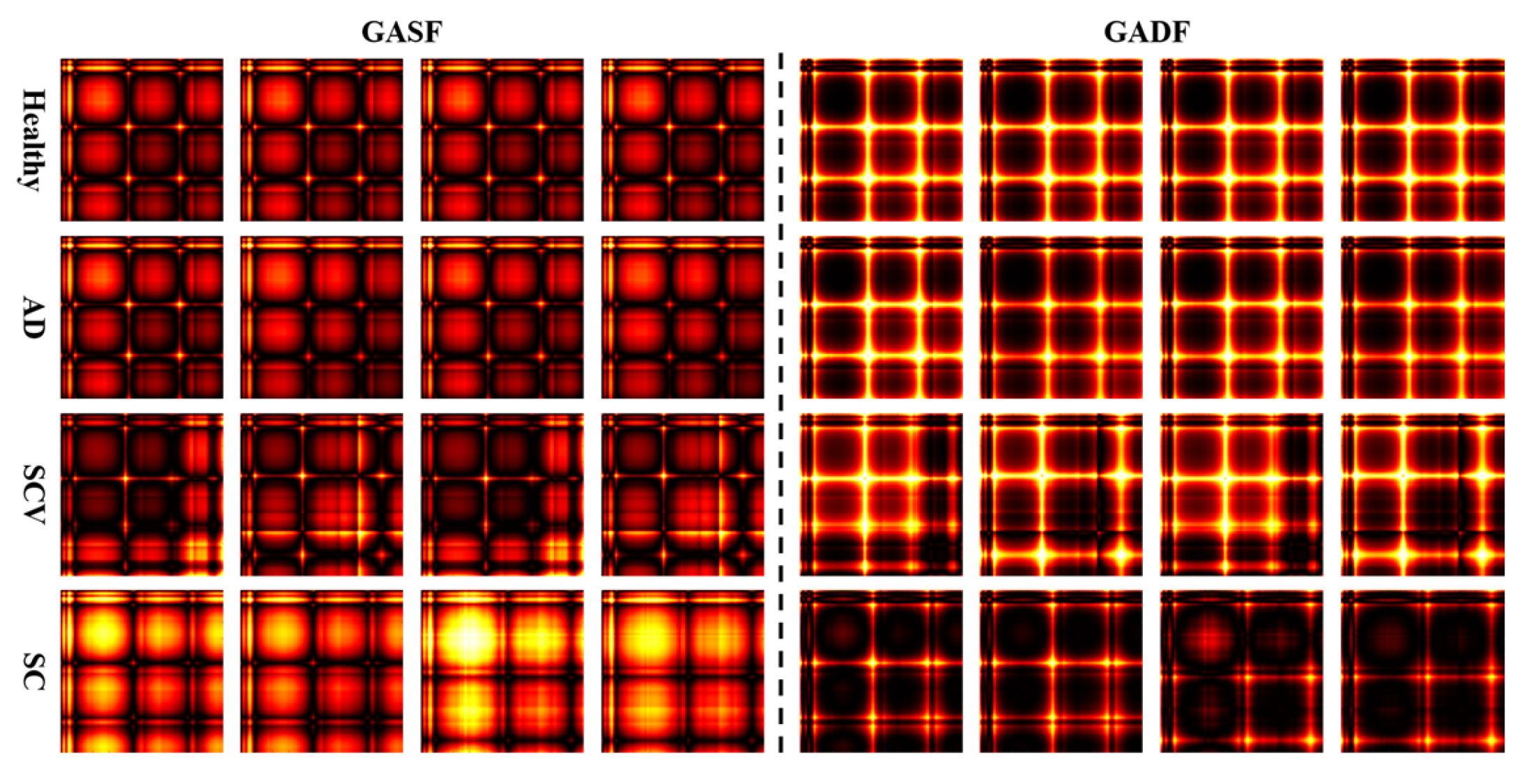
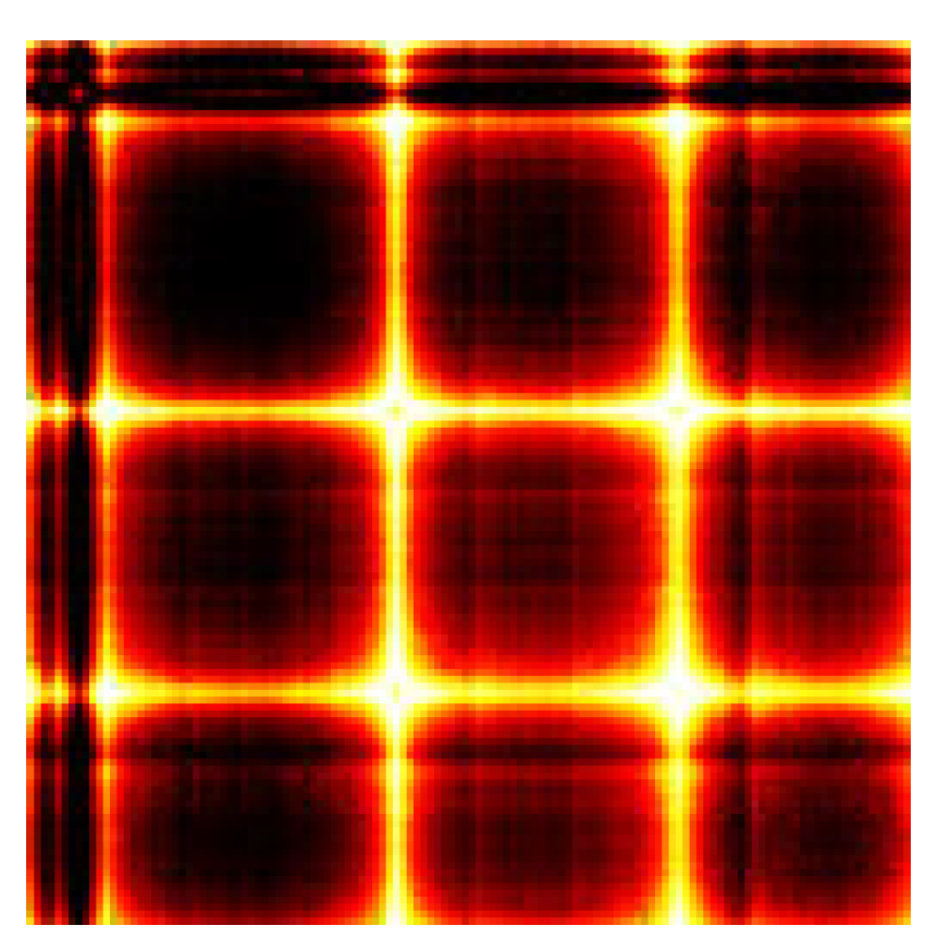
This paper uses GAF to convert transformer winding frequency response data into two-dimensional images, so that image processing algorithms can be used to extract winding fault features and complete the identification and diagnosis of transformer winding faults. The original dimensions of the GASF and GADF images converted from transformer winding frequency response data using GAF are 875 × 656 × 3. To reduce the computational burden on image processing algorithms, the dimensions of the GAF images are adjusted to 128 × 128 × 3. The processed GAF images of the frequency response curves are shown in Figure 5.
From the GASF images, it can be seen that most of the images are red and dark red, with only a small portion of other colour blocks exhibiting certain colour distribution and position distribution characteristics in the image. Under AD, the diamond-shaped orange colour blocks are primarily distributed in the upper left corner; under SCV, the diamond-shaped orange colour blocks form a square distribution in the lower right corner, and the dark red distribution shifts from the lower right to the upper left; under SC, the diamond-shaped orange colour blocks are primarily distributed in the upper left corner, and the dark red portions begin to disappear, with most of the image area turning orange.
From the GADF images, the distribution of dark red patches can be used to preliminarily determine the type of winding fault. Under AD, the upper-left dark-red dominance correlates with high-frequency attenuation from reduced inter-disc capacitance. Patch coverage scales with displacement severity. Under SCV, the upper-right concentration with lower orange streaks maps to mid-frequency phase shifts from increased turn capacitance. The strength of the stripes is directly proportional to the parallel capacitance. Under SC, the full-image darkening signifies new resonances from parasitic inductance. Darkened lower-right regions indicate fault depth.
In summary, converting the frequency response curve into a two-dimensional image provides more intuitive fault information, enabling clearer identification of the patterns between different types and degrees of winding faults. Additionally, a single frequency response curve can be converted into two images, GASF and GADF, significantly enriching the fault information and facilitating subsequent analysis and identification by deep learning networks, thereby enhancing the accuracy and effectiveness of fault detection.

4. Data Augmentation for Frequency Response Curves Based on GAF

4.1. Basic Principles and Improvements of GAN

Transformer equipment has high reliability, and winding faults are rare events, leading to a scarcity of winding fault samples and posing challenges for fault diagnosis. GAN can extract image features and use them to generate new image samples. Theoretically, GAN can address the issue of insufficient training samples, enhancing the diagnostic effectiveness of intelligent diagnostic algorithms for transformer winding faults. The basic principles of GAN include two structures: generators and discriminators. During training, generators and discriminators compete and learn from each other, continuously improving their performance through adversarial training strategies [20]. Their network structure is shown in Figure 6.
The generative network continuously combines noise to generate fake data, which are then input into the discriminative network along with the original data. The discriminative network judges the true source of the data and outputs a probability representing the authenticity of the data, which is used to adjust the weights of the generative network and the discriminative network. When the discriminative network cannot judge the authenticity of the data, an optimal data generation adversarial network model is established. The objective function of the GAN model is:
min G   max D V ( G , D ) = E x ~ p d a t a ( x ) [ log D ( x ) ] + E z ~ p z ( z ) [ log ( 1 D ( G ( z ) ) ) ]
where x is the real sample; z is the random noise vector; pdata(x) represents the latent distribution of the real sample; pz(z) represents the latent distribution of the generated sample; D() is the probability that the discriminator judges the input sample to be a real sample, which is a real number in the range 0~1; and G(z) represents the sample generated by the random noise vector.
The generator and discriminator continuously adjust their parameters through alternating iterative adversarial training until the two networks reach a dynamic Nash equilibrium, i.e., D(G(z)) = 0.5, thereby establishing the optimal adversarial network. However, due to the instability of the network structure, GAN also face challenges such as network oscillations, failure to converge, pattern collapse, and vanishing gradients during training. To address these issues, scholars and researchers have proposed improvements to the GAN network structure from various perspectives, including the Wasserstein GAN with Gradient Penalty (WGAN-GP), Deep Convolution GAN (DCGAN), and Boundary Equilibrium GAN (BEGAN), among others [21].
(1)
WGAN-GP
GANs typically use Jensen–Shannon divergence or Kullback–Leibler divergence as their loss functions. When generated and real sample distributions exhibit no overlap, the loss function gradient vanishes. This prevents updates to the generator’s weight parameters. Consequently, network training becomes infeasible. To address this issue, Arjovsky et al. optimised the loss function for GANs and proposed the Wasserstein GAN (WGAN) [22]. WGAN uses the Wasserstein distance to measure the distance between the data distributions of generated samples and real samples, with the objective function defined as:
min G   max D Δ V ( G , D ) = E x ~ p d a t a ( x ) [ D ( x ) ] E z ~ p z ( z ) [ D ( G ( z ) ) ]
where ∆ denotes the set of 1-Lipschitz functions.
However, due to the use of gradient truncation to satisfy the Lipschitz continuity constraint, WGAN may encounter issues such as the non-convergence of network parameters, poor sample quality, and mode collapse when learning the latent distribution of complex samples. To address this, Ishaan et al. further improved WGAN by incorporating a gradient penalty term (GP), proposing the WGAN-GP [23]. WGAN-GP replaces gradient clipping with a gradient penalty term, with its objective function defined as:
min G   max D V ( G , D ) = E x ~ p d a t a ( x ) [ D ( x ) ] E z ~ p z ( z ) [ D ( G ( z ) ) ] + λ E x ^ ~ P ( x ^ ) [ ( x ^ D ( x ^ ) 2 1 ) 2 ]
where λ is the gradient penalty coefficient, and x ^ is the random interpolation sampling on the line connecting two points after sampling each point on the generated samples and real samples, which is defined as:
x ^ = ε x r ( 1 ε ) x g
where xr is the real sample data, xg is the generated sample data, and ε follows a normal distribution in the range 0~1. WGAN-GP satisfies the Lipschitz continuity constraint while limiting the update range of the discriminator weight parameters, thereby avoiding the side effects introduced by gradient clipping and making the iterative training process of WGAN more stable.
(2)
DCGAN
To address the limitation of GAN’ weak generative capabilities, Radford et al. improved the structure of the GAN generator using convolutional neural networks and proposed the DCGAN based on this improvement [24]. The structure of the DCGAN generator network is shown in Figure 7. Compared to GAN, DCGAN replaces fully connected layers with convolutional layers, enhancing the generator network’s ability to capture the structural properties of the sample space; it replaces linear layers and pooling layers with strided convolutions and transposed convolutions to achieve downsampling and upsampling, thereby better preserving image details and spatial structure; and it replaces the Tanh activation function with batch normalisation (BN), which accelerates the training process while improving the stability of the generator network. These improvements significantly enhance the sample generation quality of the GAN generator.
(3)
BEGAN
The basic idea behind GAN training is to iteratively adjust the network’s weight parameters to continuously reduce the distance between the generated data distribution Pg and the real data distribution Pr. Many networks, such as WGAN-GP and DCGAN, have been developed based on this approach to improve GANs [25]. Berthelot et al. identify a challenge: directly minimizing the Pg and Pr distance in data space is often intractable. They instead propose minimizing the distance between their reconstruction distribution errors. The closer the reconstruction distribution errors of the two are, the closer their original distributions are. Based on this approach, the BEGAN was proposed [26].
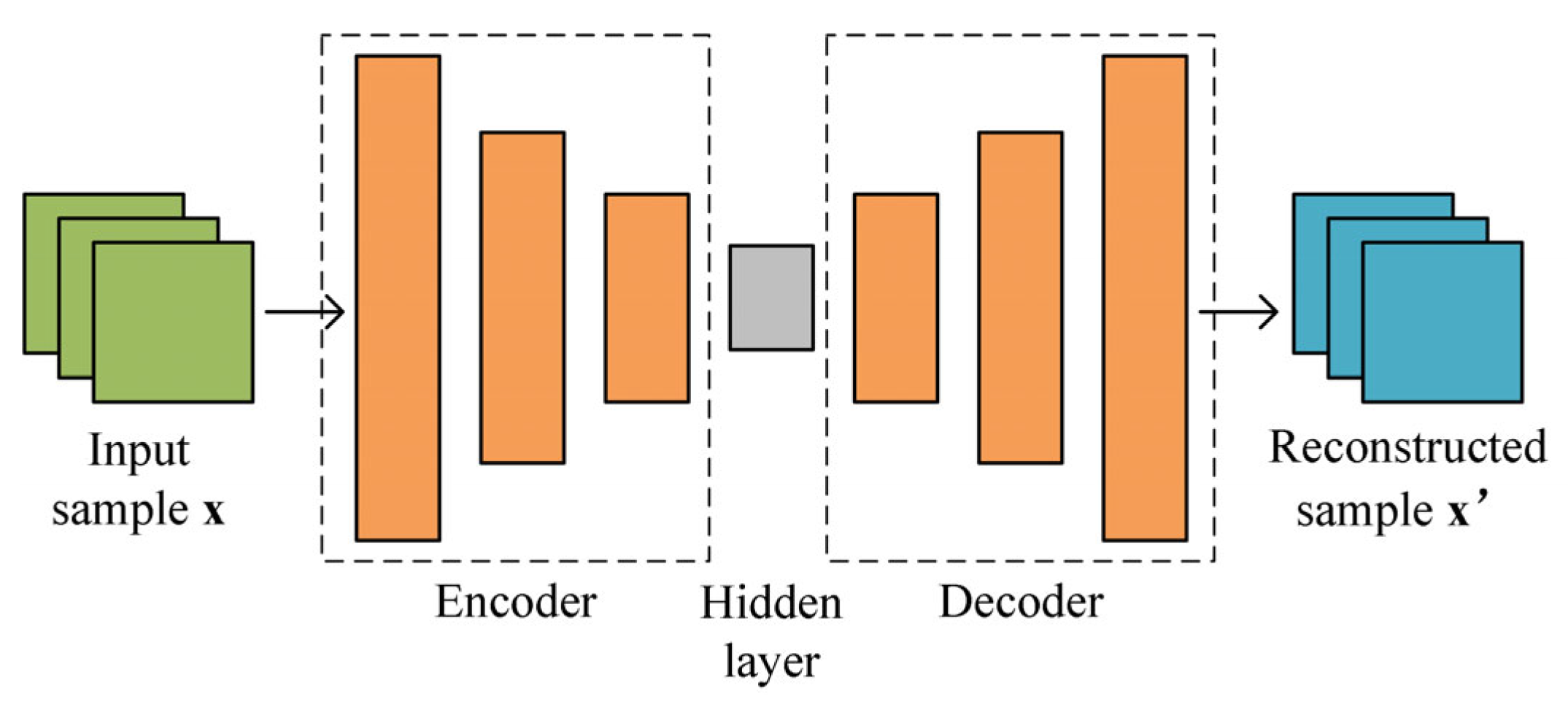
The discriminator network of BEGAN adopts an autoencoder structure, as shown in Figure 8. It converts the input sample into an intermediate vector in the hidden layer through the encoder and then converts the intermediate vector into a reconstructed sample with the same structure as the input sample through the decoder. By reconstructing the generated data distribution and the real data distribution, and using the Wasserstein distance to calculate the reconstruction distribution error [27], the formula is:
L ( v ) = v D ( v ) η
where v is the input sample data for the discriminator, and D(v) is the output sample data for discriminator D. η is the norm usage parameter, where η = 1 indicates the use of l1 norm and η = 2 indicates the use of l2 norm.
BEGAN uses boundary equilibrium conditions to improve the stability of the training process of the generative network while reducing the difficulty of convergence of the generator and discriminator weight parameters.
In summary, this paper proposes to use WGAN-GP, DCGAN, and BEGAN to augment frequency response data for transformer winding faults, with the aim of improving the diagnostic effectiveness of image recognition algorithms in such scenarios. Additionally, the paper will compare the data augmentation effects of different GAN networks to assess their suitability for fault diagnosis tasks.
Compared to other augmentation methods, VAEs generate blurry GAF images due to Gaussian prior constraints, losing high-frequency details critical for resonance identification. SMOTE operates in feature space, unsuitable for image data; its linear interpolations fail to capture nonlinear FRA distortions. While GANs outperform VAEs/SMOTE in FRA augmentation, their computational cost is higher. Future work will explore lightweight GAN variants for edge deployment.

4.2. Frequency Response Data Expansion

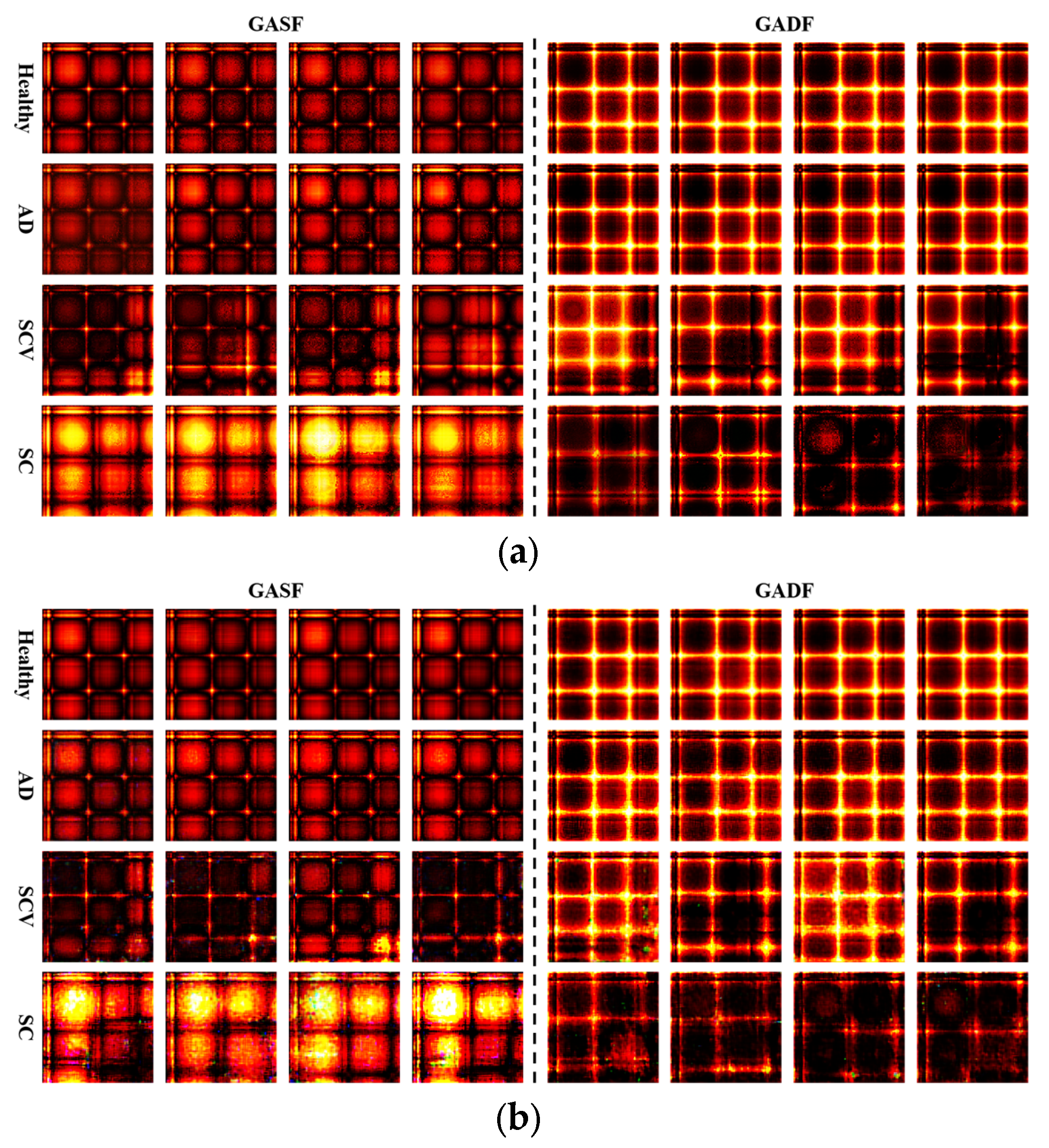
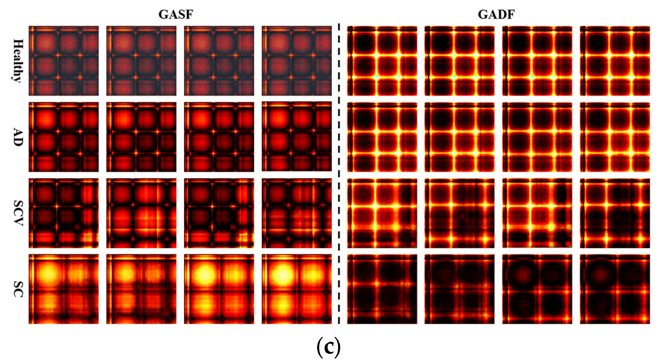
Based on the GASF and GADF images of frequency response data, this paper uses three generative adversarial networks, namely WGAN-GP, DCGAN, and BEGAN, to expand the GAF images corresponding to the frequency response data of transformer windings. Since the loss function of GAN cannot indicate the training process, in order to ensure that the network is fully trained, the WGAN-GP, DCGAN, and BEGAN networks are iteratively trained 2000 times. The GASF and GADF images generated after training the three GANs are shown in Figure 9.

4.3. Quality Assessment of GAN-Generated Samples

Structural similarity (SSIM), Peak Signal-to-Noise Ratio (PSNR), cosine similarity (CS), and Fréchet Inception Distance (FID) scores are common metrics for evaluating the quality of GAN-generated samples [28].
SSIM measures the structural similarity between images by comparing the brightness, contrast, and structural details of the real image and the generated image. It uses the mean of the image brightness as an estimate of brightness, the standard deviation as an estimate of contrast, and the covariance as a measure of structural similarity. The range of SSIM is between 0 and 1. When two images are completely identical, the SSIM value equals 1. PSNR calculates the reconstruction quality of the generated image using the mean squared error (MSE). The higher the PSNR value is, the better the reconstruction quality is of the generated image.
CS is a mathematical method commonly used to measure the similarity between two vectors. Its value ranges from −1 to 1, where 1 indicates complete similarity, −1 indicates complete opposition, and 0 indicates no similarity, as shown in Equation (11):
C S = i = 1 n A i × B i i = 1 n A i 2 × i = 1 n B i 2
FID measures the similarity between generated images and real images by comparing the feature distributions of the two. The lower the FID score is, the higher the similarity is between the generated image and the real image. When two images are identical, the FID score is 0.
This paper evaluates the quality of three types of GAN-generated images using four scoring methods: SSIM, PSNR, CS, and FID. The results are shown in Table 6.
As indicated by the SSIM metric, the generated images produced by the three generative networks exhibit structural similarities to the original images. As indicated by the PSNR metric, the reconstructed quality of the generated images produced by the three generative networks is generally good. As indicated by the CS metric, the visual similarity between the generated images produced by the three generative networks and the original images is generally high. Among them, the cosine similarity between the GASF and GADF images generated by BEGAN and the original images is above 0.8. According to the FID score, the image quality generated by BEGAN is excellent, the image quality generated by WGAN-GP is average, and the image quality generated by DCGAN is poor. DCGAN’s structural constraints (e.g., vanishing gradients) limit its effectiveness on FRA data, whereas WGAN-GP/BEGAN’s stabilization mechanisms show superior adaptability.

5. Fault Diagnosis for Windings Based on GAF–GAN–ResNet34

5.1. Residual Network

CNNs are a type of neural network model widely used in image processing and computer vision tasks. Their basic principle involves using convolutional layers to extract local features from input data, employing pooling layers to reduce data dimensions and enhance the model’s translation invariance, and finally using fully connected layers for data classification or regression. CNNs automatically learn and extract image features through convolutional operations, significantly improving the network model’s generalisation ability and performance. Due to their excellent feature extraction capabilities, CNNs have found widespread application in fields such as image classification, object detection, and facial recognition. However, as the number of layers increases, CNNs encounter issues such as gradient vanishing and network degradation during training, leading to increased training difficulty. To address this, scholars and researchers have made improvements to the network structure of CNNs, proposing various improved CNN models such as ResNet, VGGNet, DenseNet, and ShuffleNet.
Among these, ResNet introduced the residual learning mechanism, which uses skip connections to directly transmit input to deep networks, effectively alleviating the gradient vanishing and network degradation issues that arise in traditional CNNs as depth increases. Additionally, the residual structure enables the network to more easily learn and identity mappings, avoiding network degradation issues and significantly improving the training efficiency and performance of convolutional networks [29]. Depending on the number of network layers, ResNet includes variants such as ResNet18, ResNet34, ResNet50, ResNet101, and ResNet152.
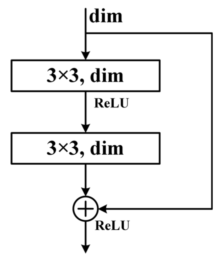
When pre-training the ResNet network using a training set composed of 128 × 128 × 3 colour images, this paper found that the ResNet34 network has a moderate parameter size, which effectively extracts image features without causing overfitting, and demonstrates good classification performance for 128 × 128 × 3 colour images. Therefore, this paper decided to use ResNet34 for transformer winding fault diagnosis research. The structural parameters of this network are shown in Table 7, where residual blocks 1–4 contain three, four, six, and three layers of residual structures, respectively, as shown in Figure 10.

5.2. Research on Winding Fault Diagnosis

The research process for winding fault diagnosis based on GAF–GAN–ResNet34 is divided into two parts: GASF image training and GADF image training. Since the GADF image training process is identical to the GASF image training process, we will use GASF image training as an example to introduce the research process for winding fault diagnosis.
(1)
Dataset Construction: Based on the GASF images obtained from the frequency response data transformation described above, we constructed the original dataset (GASF image dataset) and the GAN-augmented datasets (WGAN-GP, DCGAN, and BEGAN-augmented GASF datasets). The GASF image dataset consists of a training set, a validation set, and a test set. Each dataset includes winding frequency response images under normal conditions and three typical fault conditions. Each category of frequency response data includes 16 images; the validation set includes 4 images per category of frequency response data; the test set includes 8 images per category of frequency response data, thereby constructing the GASF image dataset. The validation set and test set of the GAN-augmented dataset are augmented with 16 real images and 24 GAN-generated images. Different GANs were used to expand the training set, thereby constructing the WGAN-expanded GASF dataset, DCGAN-expanded GASF dataset, and BEGAN-expanded GASF dataset.
(2)
Classification network training: Train the ResNet34 network on the original dataset and the GAN-augmented dataset.
(3)
Comparison of recognition accuracy: Compare the classification accuracy of the ResNet34 network trained on the GASF image dataset, the WGAN-GP-augmented GASF dataset, the DCGAN augmented GASF dataset, and the BEGAN-augmented GASF dataset to evaluate the enhancement effects of different GANs.
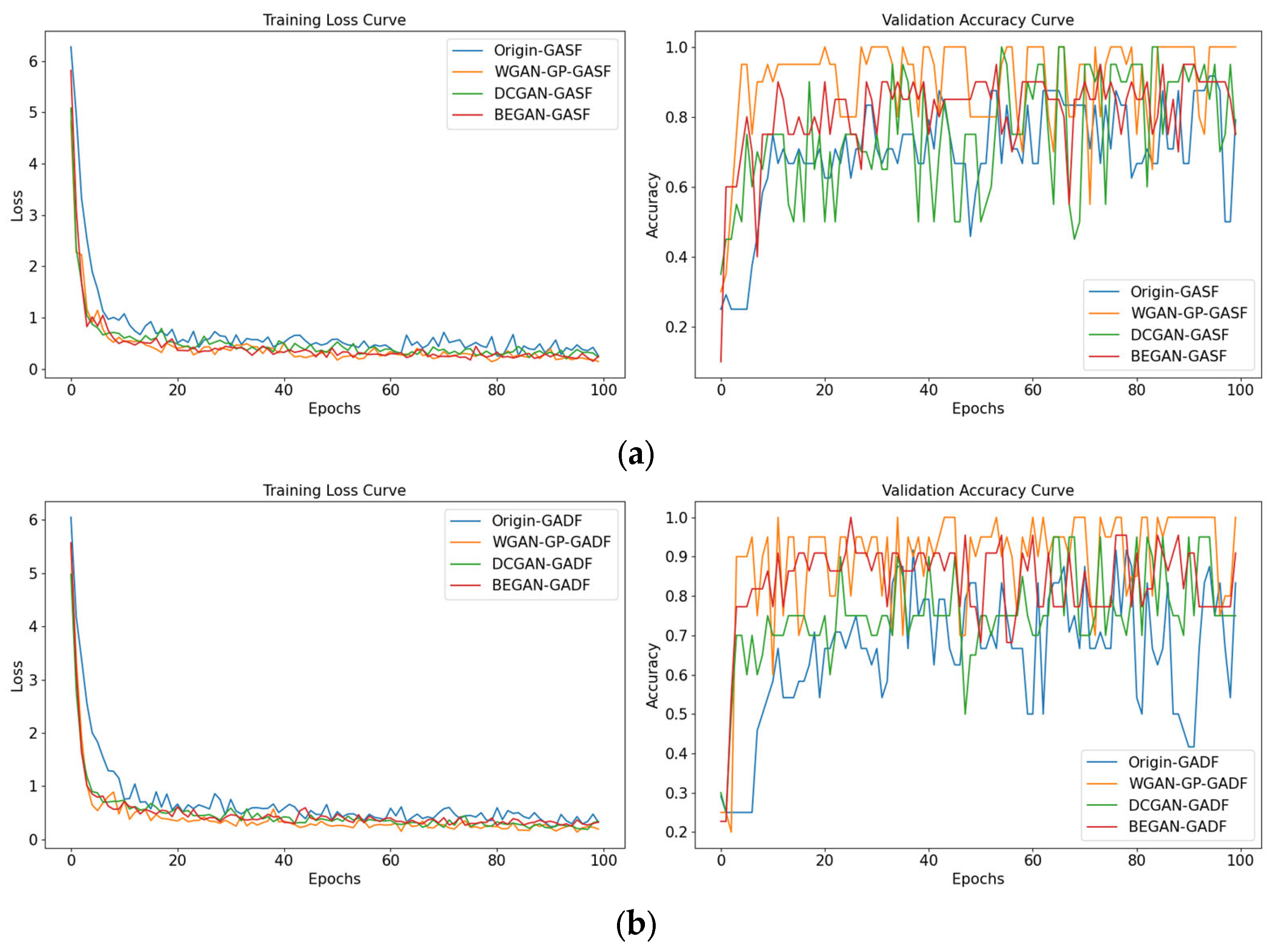
The training loss and accuracy of different GASF and GADF datasets during the training process of the ResNet34 network are shown in Figure 11. The classification accuracy of the ResNet34 classification network trained on different datasets for identifying winding faults is shown in Figure 12. From the figure, the following conclusions can be drawn: Since the frequency response images of AD are similar to those of normal windings, the classification network performs poorly in distinguishing between normal winding images and AD images before using GAN to expand the training set; both the BEGAN and WGAN-GP expanded datasets improve the classification network’s recognition accuracy, among which the most effective combination is using WGAN-GP to augment the GADF dataset. The classification network trained using this dataset achieved an identification accuracy rate of 96.88%; DCGAN, however, generates images of poor quality and lacks data augmentation capabilities, thus failing to effectively improve the classification network’s identification accuracy rate.

5.3. On-Site Case Analysis

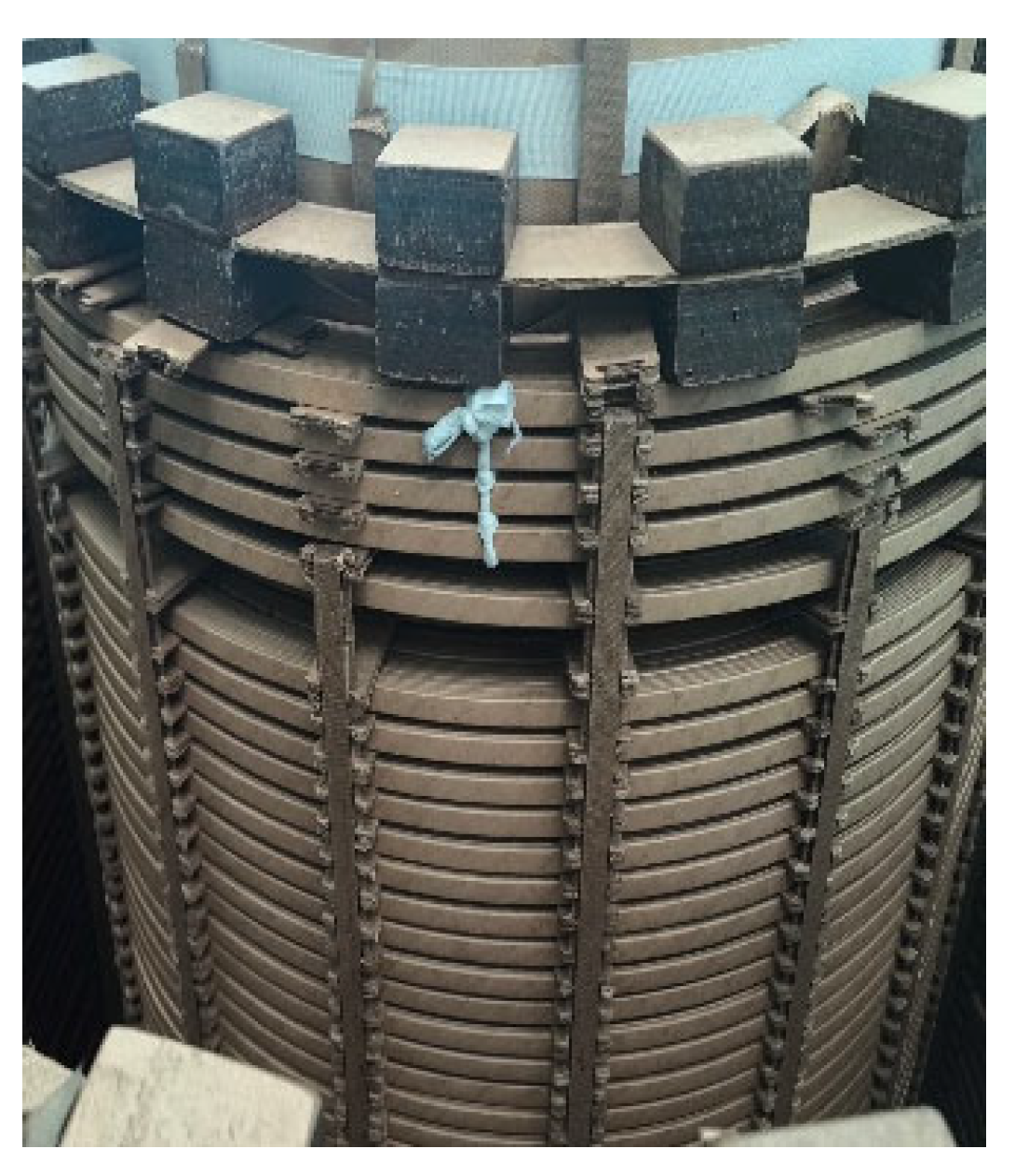
A 110 kV on-load tap-changing transformer produced by Xi’an Xibian Zhongte Electrical Equipment Co., Ltd. (Xi’an, China) was tested at a certain substation to validate the applicability of the proposed method in actual engineering scenarios, rather than adding a new test set, as shown in Figure 13a. The frequency response curves obtained from the test are shown in Figure 13b. The frequency response was converted into a GADF image using the Gram angle field, as shown in Figure 14, and this image was input into the pre-trained GADF-WGAN-GP-ResNet34 recognition model. The detection result indicated an axial displacement fault in the upper region of the winding. As shown in Figure 15, the actual fault condition of the transformer winding was found, confirming that an axial displacement fault had indeed occurred in the upper region of the winding. The output results were consistent with the actual fault, further validating the effectiveness of the method proposed in this paper and its applicability to real-world testing scenarios.

6. Conclusions

This paper obtained frequency response curves under different fault types and fault areas of windings on the simulated experimental platform. In order to address the situation of insufficient or severely insufficient sample numbers in transformer winding fault diagnosis, this paper proposes a small sample fault diagnosis method for transformer windings based on GAF–GAN–ResNet34. The results show that:
  • Since the frequency response images of AD are quite similar to those of normal windings, the classification network performed poorly in distinguishing between normal winding images and AD images before using GAN to expand the training set. DCGAN, due to its poor image generation quality, lacks data augmentation capabilities and cannot effectively improve the classification network’s recognition accuracy.
  • Both the BEGAN and WGAN-GP expanded datasets have the effect of improving the recognition accuracy of classification networks. The most effective combination is to use WGAN-GP to expand the GADF dataset. The classification network trained using this dataset achieved a recognition accuracy of 96.88%.
  • Compared to diagnostic models trained on the original dataset, the GAF-WGAN-GP-ResNet34 diagnostic model consistently achieved an accuracy rate of over 93% in identifying transformer winding fault types. Through the analysis of actual transformer fault cases and comparison with maintenance results, the effectiveness of the analysis method proposed in this paper was validated.

Author Contributions

Conceptualization, H.L. and K.Y.; methodology, H.L. and D.W.; validation, K.Y., J.H. and G.Q.; formal analysis, W.D. and D.W.; investigation, L.Z. and T.G.; resources, L.Z. and T.G.; data curation, J.S. and D.W.; writing—original draft preparation, W.D.; writing—review and editing, W.D.; visualization, H.L.; supervision, K.Y.; project administration, J.H.; funding acquisition, G.Q. All authors have read and agreed to the published version of the manuscript.

Funding

This research was funded by the Electric Power Research Institute of Yunnan Power Grid (Principle and system development of online monitoring of transformer winding faults under load-side multi-signal source excitation, YNKJXM20222300).

Data Availability Statement

The raw data supporting the conclusions of this article will be made available by the authors on reasonable request.

Conflicts of Interest

Hongwen Liu, Kun Yang, Guochao Qian, Jin Hu, Weiju Dai, Liang Zhu, Tao Guo, and Jun Shi are affiliated with Electric Power Research Institute of Yunnan Power Grid. The authors declare no conflicts of interest.

Abbreviations

The following abbreviations are used in this manuscript:
GAFGramian angular field
GANGenerative adversarial networks
ResNetDeep residual network
FRAFrequency response analysis method
GASFGramian angular summation field
GADFGramian angular difference field
ANNArtificial neural network
BPBackpropagation
CNNConvolutional neural network
BiGRUBidirectional gated recurrent unit
HVHigh-voltage
ADAxial displacement fault
SCVBulging and warping faulT
SCCake-to-cake short circuit fault
WGANWasserstein GAN
GPGradient penalty term
BNBatch normalisation
SSIMStructural similarity
PSNRPeak Signal-to-Noise Ratio
CSCosine similarity
FIDFréchet Inception Distance
MSEMean squared error

References

  1. Qian, G.; Yang, K.; Hu, J.; Liu, H.; He, S.; Zou, D.; Dai, W.; Wang, H.; Wang, D. Diagnosis Method for Transformer Winding Based on Differentiated M-Training Classification Optimized by White Shark Optimization Algorithm. Energies 2025, 18, 2290. [Google Scholar] [CrossRef]
  2. Yao, H.; Xu, Y.; Guo, Q.; Chen, S.; Lu, B.; Huang, Y. Study on Transformer Fault Diagnosisbased on Improved Deep Residual Shrinkage Network and Optimized Residual Variational Autoencoder. Energy Rep. 2025, 13, 1608–1619. [Google Scholar] [CrossRef]
  3. Zhao, X.; Yao, C.; Zhang, C.; Abu-Siada, A. Toward Reliable Interpretation of Power Transformer Sweep Frequency Impedance Signatures: Experimental Analysis. IEEE Electr. Insul. Mag. 2018, 34, 40–51. [Google Scholar] [CrossRef]
  4. Zhang, H.; Zhang, H.; Ma, Q.; Han, H.; Wang, S. Frequency Response Signature Analysis for Winding Mechanical Fault Detection of Power Transformer Using Sensitivity Method. Int. J. Appl. Electromagn. Mech. 2019, 61, 593–603. [Google Scholar] [CrossRef]
  5. Tahir, M.; Tenbohlen, S. Transformer Winding Condition Assessment Using Feedforward Artificial Neural Network and Frequency Response Measurements. Energies 2021, 14, 3227. [Google Scholar] [CrossRef]
  6. Luo, Y.; Ye, J.; Gao, J.; Chen, G.; Wang, G.; Liu, L.; Li, B. Recognition Technology of Winding Deformation Based on Principal Components of Transfer Function Characteristics and Artificial Neural Network. IEEE Trans. Dielectr. Electr. Insul. 2017, 24, 3922–3932. [Google Scholar] [CrossRef]
  7. Jayasinghe, J.A.S.B.; Wang, Z.D.; Darwin, A.W. Winding Movement in Power Transformers: A Comparison of FRA Measurement Connection Methods. IEEE Trans. Dielectr. Electr. Insul. 2006, 13, 1342–1349. [Google Scholar] [CrossRef]
  8. Samimi, M.; Tenbohlen, S.; Akmal, A.; Mohseni, H. Power Transformer Fault Diagnosis Based on Improved BP Neural Network. Electronics 2023, 12, 3526. [Google Scholar] [CrossRef]
  9. Yang, S.; Li, Z.; Yang, X.; Wu, H. Fault Identification Method of Transformer Winding based on Gramian Angular Difference Field and Convolutional Neural Network. Recent Adv. Electr. Electron. Eng. 2024, 17, 837–847. [Google Scholar] [CrossRef]
  10. Xu, Y.; Yang, X.; Xu, G.; Yang, S.; Duan, G. Transformer Fault Identification Method Based on Gramian Angle Difference Field and CNN-BiGRU. Electron. Sci. Technol. 2025, 38, 73–79. [Google Scholar] [CrossRef]
  11. Ma, X.; Tang, W.; Niu, Z.; Xin, Y. Deformation Fault Identification Method for Transformer Windings Based on Twin Convolutional Network Under Unbalanced Data Set. High Volt. Appar. 2023, 59, 120–128. [Google Scholar] [CrossRef]
  12. Duan, J.; Wu, X.; He, Y.; Song, W.; Yin, Y. Small Sample Fault Diagnosis of Transformer Windings Based on Virtual-real Feature Fusion and Data-mechanism Driven. Electr. Power Autom. Equip. 2024, 44, 212–218. [Google Scholar] [CrossRef]
  13. Chen, Y.; Zhao, Z.; Liu, J.; Tan, S.; Liu, C. Application of Generative AI-based Data Augmentation Technique in Transformer Winding Deformation Fault Diagnosis. Eng. Fail. Anal. 2024, 159, 108115. [Google Scholar] [CrossRef]
  14. Zhao, X.; Wu, G.; Yang, D.; Xu, G.; Xing, Y.; Yao, C.; Abu-Siada, A. Enhanced Detection of Power Transformer Winding Faults Through 3D FRA Signatures and Image Processing Techniques. Electr. Pow. Syst. Res. 2025, 242, 111433. [Google Scholar] [CrossRef]
  15. Zhao, X.; Yao, C.; Li, C.; Zhang, C.; Dong, S.; Abu-Siada, A.; Liao, R. Experimental Evaluation of Detecting Power Transformer Internal faults Using FRA Polar Plot and Texture Analysis. Int. J. Electr. Power Energy Syst. 2019, 108, 1–8. [Google Scholar] [CrossRef]
  16. Zhao, X.; Yao, C.; Abu-Siada, A.; Liao, R. High Frequency Electric Circuit Modeling for Transformer Frequency Response Analysis Studies. Int. J. Electr. Power Energy Syst. 2019, 111, 351–368. [Google Scholar] [CrossRef]
  17. Tang, W.; Shintemirov, A.; Wu, Q. Detection of Minor Winding Deformation Fault in High Frequency Range for Power Transformer. In Proceedings of the IEEE Power & Energy Society General Meeting, Minneapolis, MN, USA, 25–29 July 2010. [Google Scholar]
  18. Usha, K.; Usa, S. Inter Disc Fault Location in Transformer Windings Using SFRA. IEEE Trans. Dielectr. Electr. Insul. 2015, 22, 3567–3573. [Google Scholar] [CrossRef]
  19. Bian, H.; Zhang, L. Gesture Recognition Based on Gramian Angular Difference Field and Multi-stream Fusion Methods. Signal Image Video Process. 2025, 19, 120. [Google Scholar] [CrossRef]
  20. Mohammadjafari, S.; Ozyegen, O.; Cevik, M.; Kavurmacioglu, E.; Ethier, J.; Basar, A. Designing Mm-wave Electromagnetic Engineered Surfaces Using Generative Adversarial Networks. Neural Comput. Appl. 2021, 33, 11309–11323. [Google Scholar] [CrossRef]
  21. Hong, I.; Ha, J. Generative Adversarial Networks for Solving Hand-Eye Calibration Without Data Correspondence. IEEE Robot. Autom. Lett. 2025, 10, 2494–2501. [Google Scholar] [CrossRef]
  22. Zhang, C.; Feng, Y.; Qiang, B.; Shang, J. Wasserstein Generative Recurrent Adversarial Networks for Image Generating. In Proceedings of the 24th International Conference on Pattern Recognition, Beijing, China, 20–24 August 2018. [Google Scholar]
  23. Mu, D.; Meng, W.; Zhao, S.; Wang, X.; Liu, W. Intelligent Optical Communication Based on Wasserstein Generative Adversarial Network. Chin. J. Lasers 2020, 47, 217–233. [Google Scholar] [CrossRef]
  24. Gulrajani, I.; Ahmed, F.; Arjovsky, M.; Dumoulin, V.; Courville, A. Improved Training of Wasserstein GANs. In Proceedings of the 31st International Conference on Neural Information Processing Systems, Long Beach, CA, USA, 4–9 December 2017. [Google Scholar]
  25. Tang, X.; Du, Y.; Liu, Y.; Li, J.; Jia, Y.; Ma, Y. Image Recognition With Conditional Deep Convolutional Generative Adversarial Networks. Acta. Autom. Sin. 2018, 44, 855–864. [Google Scholar] [CrossRef]
  26. Li, Y.; Du, Y.; Xiao, N.; Ouyang, W. Improved Boundary Equilibrium Generative Adversarial Networks. Acta IEEE Access 2018, 6, 11342–11348. [Google Scholar] [CrossRef]
  27. Park, S.W.; Huh, J.H.; Kim, J.C. BEGAN v3: Avoiding Mode Collapse in GANs Using Variational Inference. Electronics 2020, 9, 688. [Google Scholar] [CrossRef]
  28. Tang, Y. ECGAN: Translate Real World to Cartoon Style Using Enhanced Cartoon Generative Adversarial Network. Comput. Mater. Contin. 2023, 76, 1195–1212. [Google Scholar] [CrossRef]
  29. Wu, Z.; Li, M. ResNet-Swin Transformer Based Intrusion Detection System for In-vehicle Network. Expert Syst. Appl. 2025, 279, 127547. [Google Scholar] [CrossRef]
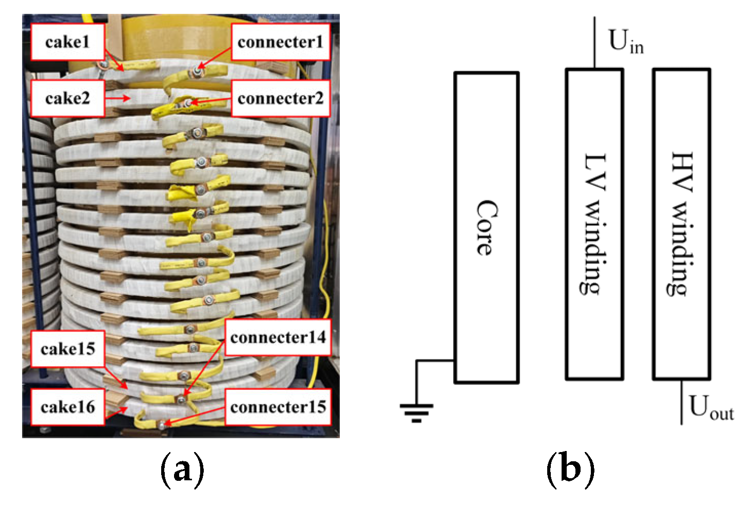
Figure 1. FRA test platform. (a) Test transformer. (b) FRA test wiring.
Energies 18 04329 g001
Figure 2. Winding fault simulation diagram. (a) AD, (b) SCV, (c) SC.
Energies 18 04329 g002
Figure 3. Iterative curves of error rate for different algorithms optimized base classifiers. (a) AD, (b) SCV, (c) SC.
Energies 18 04329 g003
Figure 4. GAF image conversion steps for frequency response curves.
Energies 18 04329 g004
Figure 5. Frequency response curve GAF image.
Energies 18 04329 g005
Figure 6. Schematic diagram of GAN structure.
Energies 18 04329 g006
Figure 7. Schematic diagram of the DCGAN generator structure.
Energies 18 04329 g007
Figure 8. Schematic diagram of the BEGAN generator structure.
Energies 18 04329 g008
Figure 9. Different GAN training results. (a) WGAN-GP, (b) DCGAN, (c) BEGAN.
Energies 18 04329 g009aEnergies 18 04329 g009b
Figure 10. Residual structure diagram.
Energies 18 04329 g010
Figure 11. Training process for different data sets.(a) Training loss and accuracy of the GASF dataset, (b) Training loss and accuracy of the GADF dataset.
Energies 18 04329 g011
Figure 12. Confusion matrix of classification networks under different training sets.
Energies 18 04329 g012
Figure 13. Field testing and result for 110 kV on-load voltage regulator transformer. (a) Field testing, (b) Test frequency response curve.
Energies 18 04329 g013
Figure 14. GADF image.
Energies 18 04329 g014
Figure 15. Field fault winding.
Energies 18 04329 g015
Table 1. Existing transformer fault diagnosis methods.
MethodAccuracySample SizeLimitations
BP Neural Network84.2%200+Slow convergence; manual features
CNN-BiGRU92.7%150Requires curve preprocessing
Twin CNN89.4%100Limited to binary faults
VAE Augmentation88.1%50Blurred high-frequency features
Proposed GAF–GAN–ResNet3496.9%28Small sample-optimized
Table 2. Fault settings for axial displacement of windings.
StructureParameterValue
HV windingNumber of line cakes16
Number of turns per coil16
Wire cake height/mm9
Wire cake width/mm34
Winding height/mm474
LV windingNumber of line cakes16
Number of turns per coil8
Wire cake height/mm9
Wire cake width/mm17
Winding height/mm474
Table 3. Fault settings for AD of windings.
NumberFaulty Line Cake PositionFault Severity
1750%
27100%
31350%
413100%
Table 4. Fault settings for SCV of windings.
NumberFaulty Joint PositionFault Severity
17, 8200 pF
27, 8560 pF
313, 14200 pF
413, 14560 pF
Table 5. Fault settings for SC of windings.
NumberFaulty Line Cake Position
15, 6
27, 8
313, 14
415, 16
Table 6. GAN image quality assessment metrics.
StructureGAN TypeSSIMPSNRCSFID
GASFWGAN-GP0.817632.790.739492.73
DCGAN0.682632.410.7026192.43
BEGAN0.673431.160.847346.49
GDSFWGAN-GP0.789632.650.83862.32
DCGAN0.7632.540.7445183.85
BEGAN0.788632.370.90231.38
Table 7. ResNet34 network structure.
Layer TypeInput DimensionOutput DimensionActivation
Function
Normalisation
Conv2d(batch_size,3,img_size,img_size)(batch_size,64,img_size/2,img_size/2)ReLUBatchNorm
MaxPool2d(batch_size,64,img_size/2,img_size/2)(batch_size,64,img_size/4,img_size/4)
Residual
Block1
(batch_size,64,img_size/4,img_size/4)(batch_size,64,img_size/4,img_size/4)ReLUBatchNorm
Residual
Block2
(batch_size,64,img_size/4,img_size/4)(batch_size,128,img_size/8,img_size/8)ReLUBatchNorm
Residual
Block3
(batch_size,128,img_size/8,img_size/8)(batch_size,256,img_size/16,img_size/16)ReLUBatchNorm
Residual
Block4
(batch_size,256,img_size/16,img_size/16)(batch_size,256,img_size/32,img_size/32)ReLUBatchNorm
Adaptive
AvgPool2d
(batch_size,256,img_size/32,img_size/32)(batch_size,512,1,1)
Reshape(batch_size,512,1,1)(batch_size,512)
Linear(batch_size,512)(batch_size,4)
Softmax(batch_size,4)(batch_size,1)ReLUBatchNorm
Disclaimer/Publisher’s Note: The statements, opinions and data contained in all publications are solely those of the individual author(s) and contributor(s) and not of MDPI and/or the editor(s). MDPI and/or the editor(s) disclaim responsibility for any injury to people or property resulting from any ideas, methods, instructions or products referred to in the content.