Research on Fault Diagnosis of High-Voltage Circuit Breakers Using Gramian-Angular-Field-Based Dual-Channel Convolutional Neural Network

Abstract

The challenge of accurately diagnosing mechanical failures in high-voltage circuit breakers is exacerbated by the non-stationary characteristics of vibration signals. This study proposes a Dual-Channel Convolutional Neural Network (DC-CNN) framework based on the Gramian Angular Field (GAF) transformation, which effectively captures both global and local information about faults. Specifically, vibration signals from circuit breaker sensors are firstly transformed into Gramian Angular Summation Field (GASF) and Gramian Angular Difference Field (GADF) images. These images are then combined into multi-channel inputs for parallel CNN modules to extract and fuse complementary features. Experimental validation under six operational conditions of a 220 kV high-voltage circuit breaker demonstrates that the GAF-DC-CNN method achieves a fault diagnosis accuracy of 99.02%, confirming the model’s effectiveness. This work provides substantial support for high-precision and reliable fault diagnosis in high-voltage circuit breakers within power systems.

1. Introduction

High-voltage circuit breakers are pivotal components within electrical power systems, playing essential roles in both the control and protection of circuits. Their reliability is directly correlated with the stability and safety of the entire power network [1,2,3]. Normally, circuit breakers remain inactive; however, during operational maneuvers or in the event of faults, they must act swiftly to either establish or disrupt the electrical supply [4,5]. Consequently, power systems impose stringent requirements on the operational reliability of high-voltage circuit breakers. Among the various operating mechanisms, spring-operated mechanisms are preferred due to their simplicity, rapid response, non-polluting nature, and compact size. These primarily include hydraulic-spring, pneumatic-spring, and fully mechanical spring mechanisms [6,7].

Currently, over 60% of circuit breaker failures are attributed to mechanical issues, such as transmission mechanism jamming, opening spring stress relaxation and buffer failure [8]. These failures generate a wealth of vibration signals during the operation of the circuit breakers, which contain extensive information about the condition of the equipment. Accurately extracting and processing these vibration signals poses a significant challenge in the field of fault diagnosis for high-voltage circuit breakers. In recent years, machine learning algorithms have been extensively studied for fault detection in circuit breakers. Notably, Support Vector Machines (SVM), Decision Trees, and Random Forests have been employed for the classification and diagnosis of mechanical faults in high-voltage circuit breakers [9,10,11]. However, these methods have limitations. Firstly, they typically rely on manually calculated features, such as time-domain and frequency-domain feature extraction, which can lead to information loss in vibration signals. Secondly, the feature representation capabilities of traditional machine learning models are limited, making it difficult to capture the deeper features within the vibration signals of circuit breakers, thereby impacting the accuracy of fault identification. In light of these issues, the rapid advancement of deep learning technologies in recent years has provided novel solutions for intelligent fault diagnosis in high-voltage circuit breakers. Compared to traditional methods, deep learning can automatically extract high-dimensional features from raw data, enhancing the accuracy of feature learning [12,13,14,15,16]. For instance, Du et al. [17] have introduced a deep residual network, which transforms one-dimensional current signals into two-dimensional grayscale images. This method employs the adaptive parameterized rectified linear activation functions and the guaranteed convergence (AMSGRAD) optimization algorithm to achieve fault diagnosis in high-voltage circuit breakers, although its accuracy is dependent on a large amount of sample data. Furthermore, the work of Yan and Huang [18,19] involved transforming vibration signals into time-frequency images for fault diagnosis using convolutional neural networks, although such representations primarily capture overall signal effects and struggle to extract instantaneous features of the signals.

Recently, Gramian Angular Field (GAF) transformations have been developed in time-series imaging for signal representation. GAF encodes one-dimensional time series into two-dimensional matrices by converting temporal dynamics into polar coordinate systems, preserving the information of amplitude and phase information [18,19]. This representation has been widely utilized in fields such as human activity recognition and biomedical diagnostics due to its ability to retain temporal correlation patterns in images [20,21]. Subsequently, Dual-Channel Convolutional Neural Networks (DC-CNNs) emerged as a powerful architecture that can process complementary inputs in parallel. Zhou et al. found that DC-CNNs—by simultaneously learning from diverse signal representations—outperform single-channel models in tasks such as power equipment classification [22]. Consequently, this study introduces a methodology that integrates the Gramian Angular Field (GAF) signal processing approach with a Dual-Channel Convolutional Neural Network (DC-CNN) for the precise extraction and analysis of transient features in signals. Specifically, this method initially converts one-dimensional vibration signals collected by sensors at five different locations on a circuit breaker into images of Gramian Angular Summation Field (GASF) and Gramian Angular Difference Field (GADF). This transformation not only augments the volume of data samples but also preserves the transient information within the signal. Subsequently, images representing each type of fault in the form of five-channel GASF and GADF images are input into two CNN modules within the DC-CNN architecture for feature extraction. The features extracted by the two CNN modules are ultimately merged to achieve high-precision fault diagnosis in high-voltage circuit breakers. The principal contributions of this research can be described through several steps. (1) Development of a GAF Representation Method (GASF + GADF): The proposed GAF-DC-CNN method is integrated with the GASF and GADF image representations via a dual-channel convolutional neural network, which is capable of effectively capturing transient features of the vibration signals. (2) Design of a DC-CNN: This network converts each fault signal into five-channel GASF and GADF images for input into convolutional networks to extract features, thereby achieving an integration of complementary signals to enhance fault diagnosis performance. (3) Comprehensive Experimental Comparison: The proposed method was compared with single-channel GAF methods (GASF-CNN, GADF-CNN) and sequence-based deep networks (CNN–LSTM). The experimental results demonstrate superior robustness and diagnostic accuracy of the proposed method.

2. Methodology

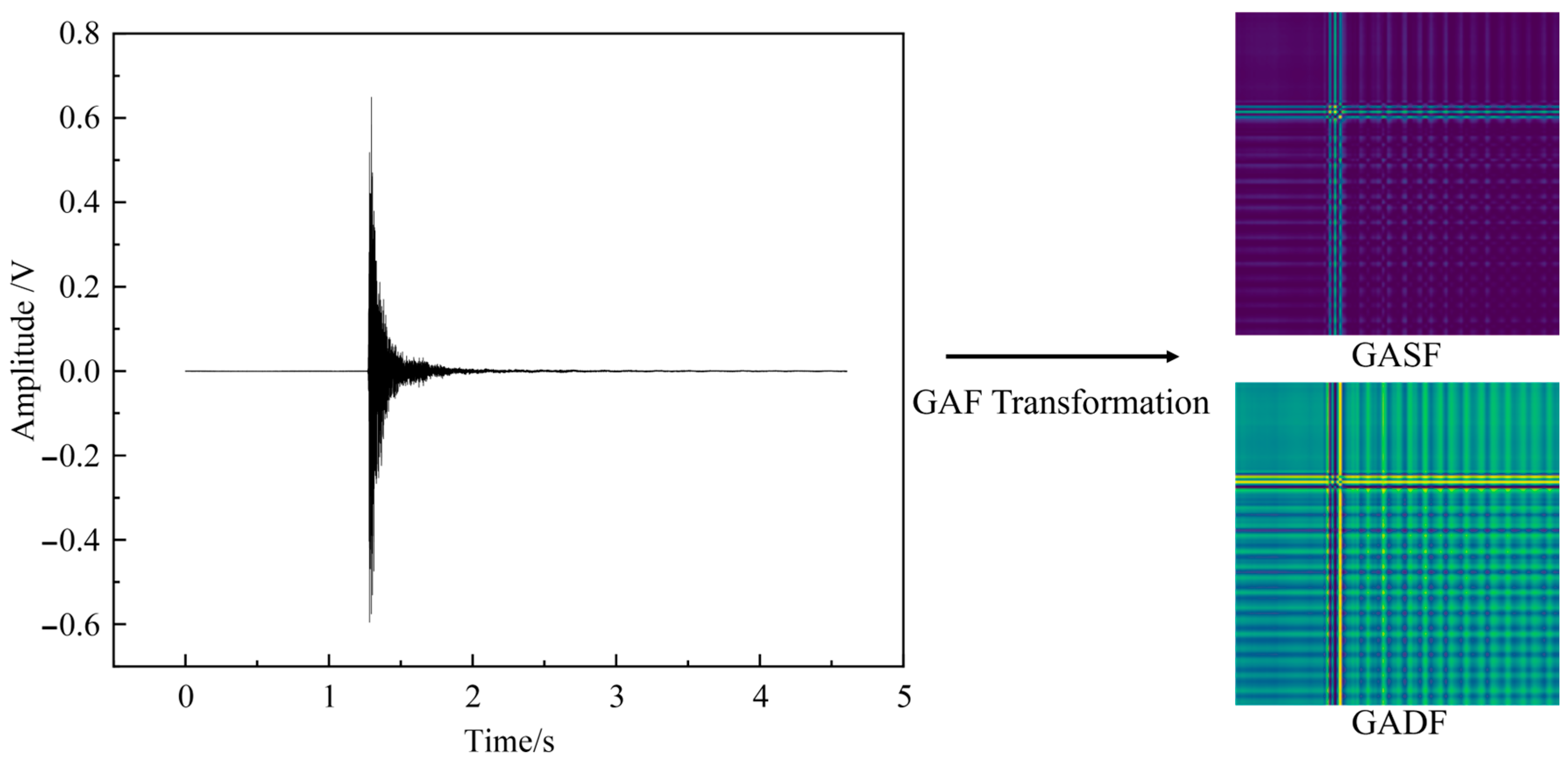
2.1. GAF Transformation

The GAF is a coding method that converts one-dimensional time series into two-dimensional images [23]. The core concept involves representing data points of a time series in Cartesian coordinates and transforming them into polar coordinates, thereby generating images through a Gram matrix based on angular relations. Specifically, given a time series of length N, {x₁, x₂, …, x_N}, the data are first normalized within the interval [−1,1] to fit the domain of the arccosine function. To avoid potential data leakage, this normalization is applied independently to each individual sample after the dataset is split into training sets and test sets. The polar coordinate angle ϕ_i is defined using Equation (1),

$$x_i=\cos ({\varphi }_i),\hspace{1em}i=1, 2, \dots , N$$

(1)

where ϕ_i ∈ [0,π].

Based on this mapping, matrices for both the GASF and GADF are constructed. The GASF utilizes the cosine of the sum of angles to define the Gram matrix G_ij, where each element is derived from the cosine of the sum of angles corresponding to time points i and j.

$$G_{ij}=\cos \left({\varphi }_i+{\varphi }_j\right),\hspace{1em}1\le i, j\le N$$

(2)

Consequently, this study explicates the intrinsic synthesis of amplitude information of a time series at moments i and j within the elements G_ij of the GASF matrix. This synthesis emphasizes the impact of phase consistency (or amplitude sign) between different time points on the matrix elements where points with identical phases (or amplitude signs) generate larger values within the matrix, reflecting the periodicity and trend similarity of the series.

GADF employs the sine function of the angular difference to define its Gram matrix, denoted as H_ij. The elements of this matrix are calculated from the sine of the angular difference between two time points.

$$H_{ij}=\sin \left({\varphi }_i-{\varphi }_j\right),\hspace{1em}1\le i, j\le N$$

(3)

Unlike the GASF, the GADF matrix is not symmetric, and its principal diagonal elements are given by sin(0) = 0, which does not directly contain the original signal’s amplitude information. Instead, the GADF matrix focuses more on the transient changes in the signal. Therefore, the values in the GADF matrix depict the short-term fluctuations and changing trends between different points in the time series, rendering it more sensitive to sudden changes, local oscillations, and other transient behaviors.

By integrating both GASF and GADF, it is possible to comprehensively characterize both static trends and dynamic changes in time series. As illustrated in Figure 1 below, one-dimensional vibration data can be transformed into two-dimensional matrix images G_ij or H_ij, which can support the input for subsequent DC-CNN processing.

2.2. Multi-Channel GAF Image Construction

In the scenario involving a single sensor, the previously mentioned GAF methodology enables the transformation of a one-dimensional vibration signal monitored by the sensor into a two-dimensional GAF image. For data derived from multiple sensors, the objective is to concurrently integrate the information from each sensor while preserving the unique characteristics of each signal. To this end, a multi-channel GAF image can be constructed by using the GASF or GADF matrices generated by each sensor as a channel, and stacking these channels to form a high-dimensional image tensor.

Here, m sensors were synchronously used to collect time-series signals that were denoted as X^(k) = {x^(k)₁, x^(k)₂, …, x^(k)_N}, where k = 1, 2, 3… represents the sensor index, and N is the length of the signal. For each sensor k, according to the definition of the GAF transformation, the GAF matrix is computed with Equation (4).

$$\begin{array}{l}{G}_{ij}^{(k)}=\cos \left({\varphi }_i^{(k)}+{\varphi }_j^{(k)}\right)\\ H_{ij}^{(k)}=\sin \left({\varphi }_i^{(k)}-{\varphi }_j^{(k)}\right), 1\le i, j\le N\end{array}$$

(4)

When constructing the multi-channel image, each sensor’s matrix serves as a channel in the fusion process. The multi-channel GASF image is represented by Equation (5).

$${\vartheta }_{GASF}(i,j,k)=\cos \left({\varphi }_i^{(k)}+{\varphi }_j^{(k)}\right),k=1, 2, \dots m$$

(5)

Similarly, the multi-channel GADF image is represented by Equation (6).

$${\vartheta }_{GADF}(i,j,k)=\sin \left({\varphi }_i^{(k)}-{\varphi }_j^{(k)}\right),k=1, 2, \dots m$$

(6)

In these equations, i and j denote the spatial positions within the image, and k indicates the corresponding channel (sensor dimension). Through this methodology, the two-dimensional angular field feature maps from m sensors are merged together, yet they remain independently preserved in distinct channels.

This method of multi-channel data fusion offers significant advantages in terms of information retention and feature extraction. On one hand, the original temporal information of each sensor, after undergoing the GAF transformation, is completely preserved within its respective channel without loss of detail or mutual interference. Compared to simplistic signal merging or dimensionality reduction, the multi-channel representation ensures that key patterns from all sensors are presented, thereby avoiding potential information loss that might occur in a single-channel approach. On the other hand, the multi-channel GAF images provide a rich and structured input for subsequent feature extraction. In the form of images, advanced pattern recognition techniques such as two-dimensional convolution can be utilized to learn features across the model that can extract temporal pattern features within each sensor sequence in individual channels, and also capture correlations and complementary information between different sensor signals through cross-channel convolutional kernels. This means that multi-channel GAF fusion not only preserves the independent information of each sensor but also provides an opportunity for algorithms to explore inter-sensor feature relationships, thus enhancing the effectiveness of pattern recognition and classification.

2.3. Evaluation Metrics

To quantitatively evaluate the performance of the proposed GAF-DC-CNN model and compare it with baseline models, three typical classification metrics such as recall (R), F1 score, and AUC (area under curve) are adopted. These metrics provide a comprehensive assessment of classification effectiveness, especially in multi-class and imbalanced datasets.

Recall, also known as sensitivity, is widely used to measure the proportion of correctly predicted positive samples [24] and is defined as in Equation (7),

$$R=TP/(TP+FN)$$

(7)

where TP (true positives) represents the number of correctly predicted fault cases, and FN (false negatives) represents the number of actual fault cases that were incorrectly classified.

The F1 score is the harmonic mean of precision and recall, as given by Equation (8),

$$F1=2\times (P\times R)/(P+R)$$

(8)

where precision P is defined as

$$P=TP/(TP+FP)$$

(9)

where FP denotes the number of incorrectly predicted fault cases.

The AUC is used to evaluate the model’s capability to distinguish fault cases at various threshold settings. For multi-class problems, AUC can be calculated to process the overall multi-class classification as a set of binary decisions,

$$AUC=(1/N)\times {\displaystyle \sum AUC(y_i,}{\widehat{y}}_i)$$

(10)

where y_i is the true label, ŷ_i is the predicted probability of the positive class for the i-th sample, and N is the total number of samples across all classes.

3. Fault Identification Method Based on GAF-DC-CNN

3.1. Vibration Data Collection and GAF Processing

Given the significance of the disengagement operation for the electrical grid’s safety, especially as high-voltage circuit breakers typically remain in a closed state for extended periods, it is essential to gather one-dimensional vibration data from high-voltage circuit breakers under various fault conditions during disengagement. Taking the CT26 spring-operated mechanism of a 220 kV circuit breaker as an example, vibration data under different operational conditions were collected using five LZ-601 accelerometers (as illustrated in Figure 2). These sensors, with a sensitivity of 10.0 mV/g, were set to collect data at a frequency of 10 kHz. Prior studies suggest that the sampling rate for vibration signals from high-voltage circuit breakers usually ranges between 8 and 16 kHz [25,26]. Pre-tests conducted on five typical mechanical failures—sticking drive mechanisms, relaxation of disengagement springs, abnormal core stroke or gap, and damper faults—using an oversampling rate of 25 kHz revealed a peak significant frequency of 4.7 kHz. According to the Nyquist criterion, a sampling rate of 10 kHz accurately captures all characteristic frequencies, balancing data volume with storage and training efficiency.

To effectively extract vibration characteristics of the high-voltage circuit breaker under different fault conditions, it is necessary to carry out feature transformations on the collected one-dimensional time series data to enhance the accuracy of subsequent fault identification. Initially, the collected signals are normalized to mitigate the impact of varying scales and to ensure that the data distribution is suitable for GAF encoding. Subsequently, the normalized signals are mapped to the angular domain, and two-dimensional feature matrices are constructed using GASF and GADF methods, respectively. GASF primarily captures global features of the signal, whereas GADF focuses on depicting local changes in the signal pattern. Figure 3 presents the GASF and GADF images derived from the vibration signals from six operational conditions, (a) normal operation, (b) transmission mechanism jamming, (c) opening spring stress relaxation, (d) abnormal core stroke, (e) abnormal core gap, and (f) buffer failure. These images encode the temporal correlation of vibration signals using angular-based transformations. Therefore, subtle variations such as localized distortions in texture patterns resulting from various operational conditions can be obtained to reflect different dynamic behaviors of the circuit breaker. These differences can be captured through the feature extraction using the convolutional neural network, enabling accurate fault classification.

3.2. Construction of DC-CNN

Traditional CNN architectures typically support only a single type of data input, which poses challenges in directly processing multiple, distinct data types. For the GAF transformation, which comprises GASF and GADF image representations, using these images as inputs for a standard CNN for feature extraction and classification could be hindered by the network’s architectural constraints, thereby not fully leveraging the information from both types of images.

To address this issue, a DC-CNN that consists of two independent CNN branches is proposed to process either GASF or GADF images as shown in Figure 4. After each CNN module extracts features from its respective inputs, a feature fusion strategy is employed to integrate this information, ultimately aiding in classification. At the network’s input layer, data are formatted as multi-channel images with dimensions H × W × C, where H and W represent the height and width of the image, respectively, and C denotes the number of channels, corresponding to the number of vibration signals collected by multiple sensors under the same operational conditions. The input data are GASF and GADF images derived from the GAF methodology, standardized in height and width to maintain uniformity in subsequent CNN processing.

During the feature extraction phase, each CNN branch comprises multiple convolutional and pooling layers. The convolutional layers utilize a sliding window mechanism on the input feature maps for local perception, thus extracting spatial structural information and identifying key patterns [26]. To reduce computational complexity while preserving essential feature information, the pooling layers employ a max pooling strategy, selecting the maximum value within a local region as the feature output [27,28]. Additionally, batch normalization is introduced following the convolutional and pooling layers to accelerate model convergence and reduce internal covariate shift.

In the backend of the network, global average pooling (GAP) is incorporated to enhance the model’s capability for feature representation. Unlike max pooling, GAP does not select extremes in a local area but computes a global average across the entire feature map, mapping high-dimensional features of each channel to a single scalar. This strategy effectively reduces the model’s parameter count, thereby decreasing the risk of overfitting, and also enhances the global expression of features.

A critical aspect of the DC-CNN is the choice of feature fusion strategy. Common methods include direct concatenation, weighted summation, and element-wise multiplication. Direct concatenation preserves the entirety of the feature information extracted by both CNN branches; therefore, this method is utilized in this study to enhance the model’s joint representational capacity for different input data and improve classification performance.

The specific network structure and parameter configurations involved in the implementation of the DC-CNN are detailed in

Table 1. Structural parameters of DC-CNN.

Layer Name	Number of Channels	Convolution Kernel/Pooling Window Size	Stride Length	Output Dimensions	Padding
GADF:
Input	5	—	—	128 × 128 × 5	—
Conv_1	48	5 × 5	1	128 × 128 × 48	SAME
Conv_2	96	4 × 4	1	128 × 128 × 96	SAME
MaxPool_1	96	2 × 2	2	64 × 64 × 96	—
Conv_3	128	3 × 3	1	64 × 64 × 128	SAME
Conv_4	192	3 × 3	1	64 × 64 × 192	SAME
MaxPool_2	192	2 × 2	2	32 × 32 × 192	—
Conv_5	256	3 × 3	1	32 × 32 × 256	SAME
MaxPool_3	256	2 × 2	2	16 × 16 × 256	—
Global Average Pooling	256	16 × 16	—	1 × 1 × 256	—
FC_1	—	—	—	256	—
GASF:
Input	5	—	—	128 × 128 × 5	—
Conv_6	48	5 × 5	1	128 × 128 × 48	SAME
Conv_7	96	4 × 4	1	128 × 128 × 96	SAME
MaxPool_4	96	2 × 2	2	64 × 64 × 96	—
Conv_8	128	3 × 3	1	64 × 64 × 128	SAME
Conv_9	192	3 × 3	1	64 × 64 × 192	SAME
MaxPool_5	192	2 × 2	2	32 × 32 × 192	—
Conv_10	256	3 × 3	1	32 × 32 × 256	SAME
MaxPool_6	256	2 × 2	2	16 × 16 × 256	—
Global Average Pooling	256	16 × 16	—	1 × 1 × 256	—
FC_2	—	—	—	256	—
Integration layer: direct connection method
FC_3	—	—	—	512	—
FC_4	—	—	—	256	—
Output	—	—	—	6	—

. During the training phase, the Adam (Adaptive Moment Estimation) optimizer is employed for parameter updates, with the cross-entropy loss function serving as the objective function. The Adam optimizer is an adaptive gradient-based optimization algorithm that computes individual learning rates for each parameter by combining the advantages of momentum and root mean square propagation (RMSProp). It is widely used in signal processing and image recognition due to its fast convergence and high stability in deep learning applications [29,30]. The initial learning rate is set at 0.0005, and L2 regularization is utilized to mitigate overfitting, with a regularization coefficient of 0.01. These hyperparameters are determined based on experimental data to ensure the model’s generalization capability. The convolutional and pooling layer configurations of the GASF and GADF branches are designed to be symmetric, which enables consistent feature extraction and facilitates effective feature fusion.

In the data preprocessing stage, data from each operational condition are collected by five sensors, accumulating a total of 2400 one-dimensional data points across six conditions, five sensors, and 80 disengagement operations. After undergoing the GAF transformation, this results in 4800 images with a resolution of 128 × 128, representing both GASF and GADF. These images, combined with multi-channel inputs from five sensors, form a dataset of 960 five-channel image samples. These samples are fed into the two independent channels of the CNN to thoroughly mine key information from different images.

4. Results

In this work, a comparative analysis with three models—CNN–LSTM, GADF-CNN, and GASF-CNN—was carried out. The CNN–LSTM model, which integrates a one-dimensional CNN with Long Short-Term Memory (LSTM) networks, is particularly adept at classifying time-series data. Thus, it is employed as a baseline model to explore the impact of the GAF transformation on enhancing classification performance. Concurrently, to further assess the efficacy of GAF-DC-CNN in diagnosing faults in high-voltage circuit breakers, GADF-CNN and GASF-CNN, which are single-channel neural network architectures, serve as comparative models. An in-depth comparison of the GADF and GASF transformations in classification tasks is undertaken to evaluate their differences in feature representation and classification capabilities.

The datasets of GAF images representing normal states and various faults, such as CT-26 transmission mechanism stickiness, disengagement spring stress relaxation, abnormal disengagement iron core stroke, irregular disengagement iron core gap, and CT-26 buffer faults, are divided into training and test sets in an 8:2 ratio. The CNN–LSTM is trained using the original one-dimensional vibration data, while GADF-CNN and GASF-CNN are trained with the GADF image dataset and GASF image dataset, respectively, and the proposed GAF-DC-CNN model is trained using the multi-channel GAF image dataset. Figure 5 displays the accuracy changes in the test set during the training process for all four models. From the accuracy curves, it is evident that the CNN–LSTM model exhibits a slower convergence speed and lower test set accuracy compared to the other three models, stabilizing after approximately 500 iterations. In contrast, the other three models tend to stabilize after just 300 iterations, illustrating the enhancements in convergence speed and accuracy brought about by the GAF transformation.

To verify the effectiveness of the GAF-DC-CNN, this study assesses four models using accuracy, recall, F1 score, and AUC from the test dataset. The AUC is used to measure a model’s ability to differentiate between positive and negative class samples across various classification thresholds. For multi-class tasks, this research adopts a “micro-average” approach for calculating the AUC, treating the issue as a global binary classification problem. By aggregating the prediction outcomes across all categories, a single AUC value is computed to evaluate the overall performance of the model. An AUC value closer to 1 indicates superior overall classification performance and a stronger ability to discriminate among fault categories.

As shown in

Table 2. Evaluation metrics for the four models.

Model	Accuracy	Recall	F1 Score	AUC
GAF-DC-CNN	0.9902	0.9971	0.9841	0.9962
GADF-CNN	0.9523	0.9602	0.9547	0.9974
GASF-CNN	0.9234	0.9211	0.9484	0.9893
CNN–LSTM	0.9004	0.8919	0.9084	0.9692

, the results, indicate a performance trend of GAF-DC-CNN > GADF-CNN > GASF-CNN > CNN–LSTM across the four evaluation metrics. Notably, the GAF-DC-CNN model achieved a recognition accuracy of 0.9902, demonstrating the highest accuracy in the identification of faults in high-voltage circuit breakers, while the CNN–LSTM only reached an accuracy of 0.9004. Moreover, the calculation of recall is based on the weighted average of fault recognition results, ensuring that it reflects the overall model’s capability to classify types of spring faults. Overall, the GAF-DC-CNN model presents the best performance, illustrating the enhancements in classification ability conferred by the GAF transformation and the DC-CNN architecture. The confusion matrix of the GAF-DC-CNN model on the test set is shown in Figure 6, and a high classification accuracy across all fault types was achieved. It can be found that each fault category is classified with high accuracy from 97.90% to 100%, and the average per-class accuracy is 99.02%, which indicates that the GAF-DC-CNN model is feasible in accurately identifying any single fault type occurring in a CT26 operating mechanism.

To further verify the viability of the proposed GAF-DC-CNN model, we conducted five-fold cross-validation on the entire dataset. The dataset was randomly partitioned into five equal-sized folds, where each fold served once as the test set and the remaining four folds as the training set. This procedure was repeated for five times in total, and the performance metrics were averaged across all folds.

Table 3. Performance metrics of the GAF-DC-CNN model under five-fold cross-validation.

Metric	Mean Value	Standard Deviation
Accuracy	0.9984	±0.0042
Recall	0.9943	±0.0031
F1 Score	0.9827	±0.0038
AUC	0.9951	±0.0026

presents the averaged results of accuracy, recall, F1 score, and AUC. The results show that the proposed model maintains high classification performance with low variance, indicating its strong generalizability across various data splits.

5. Conclusions

In this study, a GAF-DC-CNN approach was proposed to address the non-stationary characteristics of vibration signals in high-voltage circuit breakers and the limitations of traditional methods in fault diagnosis. By employing dual-channel feature extraction through GASF and GADF, the GAF-DC-CNN effectively captures both global trends and local dynamic characteristics of variation signals, significantly enhancing the diagnostic accuracy for mechanical failures in circuit breakers. Experimental results revealed that the GAF-DC-CNN achieved an overall classification accuracy of 99.02% under six representative operating conditions of a 220 kV circuit breaker. The confusion matrix further demonstrated consistently high per-class accuracies ranging from 97.90% to 100%, verifying the model’s balanced discrimination capability across diverse fault types. Additionally, the robustness and generalization performance of the proposed method were validated through five-fold cross-validation, yielding an average accuracy of 99.84%. These findings substantiate the effectiveness of incorporating GAF transformations for fault identification in high-voltage circuit breakers and highlight the enhanced stability and reliability conferred by the dual-channel architecture. Thus, the proposed GAF-DC-CNN method provides an efficient and reliable intelligent analysis tool for diagnosing mechanical failures in high-voltage circuit breakers, facilitating the advancement of automation and intelligence in power system equipment condition monitoring.

References

1. Liu, Y.; Zhang, G.; Zhao, C.; Lei, S.; Qin, H.; Yang, J. Mechanical condition identification and prediction of spring operating mechanism of high voltage circuit breaker. IEEE Access 2020, 8, 210328–210338. [Google Scholar] [CrossRef]
2. Yang, M.; Wei, L.; Qiu, P.; Hu, G.; Yang, K.; He, X.; Peng, Z.; Zhou, F.; Zhang, Y.; Luo, J.; et al. Evaluation on the Long-Term Operational Reliability of Closing Springs in High-Voltage Circuit Breakers. Energies 2025, 18, 1806. [Google Scholar] [CrossRef]
3. Razi-Kazemi, A.A.; Niavesh, K. Condition monitoring of high voltage circuit breakers: Past to future. IEEE Trans. Power Deliv. 2020, 36, 740–750. [Google Scholar] [CrossRef]
4. Zhu, Y.; Jiang, Y.; Cao, F.; Wang, P.; Ke, J.; Liu, J.; Nie, Y.; Li, G.; Wei, Y.; Lu, G.; et al. Space charge induced electrofluorochromic behavior for C12-BTBT based thin-film devices. J. Mater. Chem. C 2025, 13, 12027. [Google Scholar] [CrossRef]
5. Su, Y.; Lu, Y.; Xie, Z.; Wang, J.; Luo, C. Study on closing spring fatigue characteristics of high voltage circuit breaker. IOP Conf. Ser. Earth Environ. Sci. 2020, 508, 012174. [Google Scholar] [CrossRef]
6. Zhao, X.; Wu, G.; Yang, D.; Xu, G.; Xing, Y.; Yao, C.; Abu-Siada, A. Enhanced detection of power transformer winding faults through 3D FRA signatures and image processing techniques. Electr. Pow. Syst. Res. 2025, 242, 111433. [Google Scholar] [CrossRef]
7. Wan, S.; Chen, L. Fault diagnosis of high-voltage circuit breakers using mechanism action time and hybrid classifier. IEEE Access 2019, 7, 85146–85157. [Google Scholar] [CrossRef]
8. Shao, H.; Jiang, Y.; Zhao, J.; Yang, M.; Wang, X.; Yang, H. Hybrid multi-scale residual network for high-voltage circuit breakers fault diagnosis. Electron. Lett. 2025, 61, e70135. [Google Scholar] [CrossRef]
9. Liu, M.; Wang, K.; Sun, L.; Zhen, J. Applying empirical mode decomposition (EMD) and entropy to diagnose circuit breaker faults. Optik 2015, 126, 2338–2342. [Google Scholar] [CrossRef]
10. Wu, L. Research on Fault Diagnosis and Maintenance Decision of High Voltage Circuit Breaker. Master’s Thesis, Tianjin University, Tianjin, China, 2019. [Google Scholar]
11. Ji, T.; Yi, L.; Tang, W.; Shi, M.; Wu, Q. Multi-map fault diagnosis of high voltage circuit breaker based on mathematical morphology and wavelet entropy. CSEE J. Power Energy Syst. 2019, 5, 130–138. [Google Scholar] [CrossRef]
12. Huang, N.; Chen, H.; Cai, G.; Fang, L.; Wang, Y. Mechanical fault diagnosis of high voltage circuit breakers based on variational mode decomposition and multi-layer classifier. Sensors 2016, 16, 1887. [Google Scholar] [CrossRef] [PubMed]
13. Sun, L. Research on Deep Residual Network Model and Its Application in Circuit Breaker Fault Diagnosis. Master’s Thesis, Hebei University of Technology, Hebei, China, 2023. [Google Scholar]
14. Xu, J.; Zhang, B.; Lin, X.; Li, B.; Teng, Y. Application of energy spectrum entropy vector method and RBF neural networks optimized by the particle swarm in high-voltage circuit breaker mechanical fault diagnosis. High Voltage Eng. 2012, 38, 1299–1306. [Google Scholar]
15. Zhao, K.; Yang, J.; Ma, S.; Wang, Y.; Wu, J.; Liang, C. Application of neural network ensemble model in mechanical fault identification of high voltage circuit breaker. High Volt. Appar. 2018, 54, 217–223. [Google Scholar]
16. Zhao, L.; Ji, Y.; Wu, Y.; Wu, X.; Ning, W.; Huang, X.; Ren, J. LM-BP fault diagnosis algorithm for spring operating mechanism of high voltage circuit breaker based on motor current. Electr. Meas. Instrum. 2024, 61, 48–55. [Google Scholar]
17. Du, T.; Sun, L.; Sun, S.; Chen, F.; Liu, J. Application of deep residual network in circuit breaker fault diagnosis. Instrum. Technol. Sensor 2022, 7, 95–99. [Google Scholar]
18. Yan, R.; Lin, C.; Gao, S.; Luo, J.; Li, T.; Xia, Z. Fault diagnosis and analysis of circuit breaker based on wavelet time-frequency representations and convolutional neural network. J. Vib. Shock. 2020, 39, 198–205. [Google Scholar]
19. Huang, X.; Hu, X.; Zhu, Y.; Wei, X.; Zhou, Y.; Gao, H. Fault diagnosis of high voltage circuit breaker based on convolutional neural network. Electr. Power Autom. Equip. 2018, 38, 136–140. [Google Scholar]
20. Xu, H.; Li, J.; Yuan, H.; Liu, Q.; Fan, S.; Li, T.; Sun, X. Human activity recognition based on Gramian angular field and deep convolutional neural network. IEEE Access 2020, 8, 199393–199405. [Google Scholar] [CrossRef]
21. Zhang, G.; Si, Y.; Wang, D.; Yang, W.; Sun, Y. Automated detection of myocardial infarction using a Gramian angular field and principal component analysis network. IEEE Access 2019, 7, 171570–171583. [Google Scholar] [CrossRef]
22. Zhou, F.; Ma, Y.; Wang, B.; Lin, G. Dual-channel convolutional neural network for power edge image recognition. J. Cloud Comp. 2021, 10, 18. [Google Scholar] [CrossRef]
23. Peng, W.; Zhang, G. Research on fault diagnosis of low-voltage circuit breaker based on vibration and coil current signals. Adv. Technol. Electr. Eng. Energy 2025, 44, 106–115. [Google Scholar]
24. Hossain, M.A.; Sajib, M.S.A. Classification of image using convolutional neural network (CNN). Glob. J. Comput. Sci. Technol. 2019, 19, 13–14. [Google Scholar] [CrossRef]
25. Cao, J.; Chen, S.; Bao, X.; Cong, L.; Zhou, J. Research on fault diagnosis of circuit breakers based on spectrograms and improved residual networks. Mach. Electron. 2025, 43, 9–15. [Google Scholar]
26. Wang, X.; Wang, X.; Jia, X.; Zhang, F.; Li, S.; Hu, Y. Fault identification method of outage transmission line based on convolutional neural network and wavelet packet decomposition. Electr. Meas. Instrum. 2025, 62, 61–67. [Google Scholar]
27. Razavi-Far, R.; Chakrabarti, S.; Saif, M.; Zio, E. An integrated imputation-prediction scheme for prognostics of battery data with missing observations. Expert. Syst. Appl. 2019, 115, 709–723. [Google Scholar] [CrossRef]
28. Song, J.; Wang, H.; Du, M.; Peng, L.; Zhang, S.; Xu, G. Non-intrusive load identification method based on improved long short term memory network. Energies 2021, 14, 684. [Google Scholar] [CrossRef]
29. Kingma, D.P.; Ba, J. Adam: A method for stochastic optimization. In Proceedings of the 3rd International Conference on Learning Representations, San Diego, CA, USA, 7–9 May 2015. [Google Scholar]
30. Cong, S.; Zhou, Y. A review of convolutional neural network architectures and their optimizations. Artif. Intell. Rev. 2023, 56, 1905–1969. [Google Scholar] [CrossRef]
Figure 1. GAF transformation of vibration signal.
Energies 18 03837 g001
Figure 2. Vibration signal collection system of the spring-operated mechanism.
Energies 18 03837 g002
Figure 3. GAF images corresponding to different operational conditions.
Energies 18 03837 g003
Figure 4. Schematic of the fault identification method based on GAF-DC-CNN.
Energies 18 03837 g004
Figure 5. Accuracy curves of the test sets for the four models.
Energies 18 03837 g005
Figure 6. Confusion matrix of the GAF-DC-CNN model (accuracy in %). Fault classes: a: normal operation, b: transmission mechanism jamming, c: opening spring stress relaxation, d: abnormal core stroke, e: abnormal core gap, f: buffer failure.
Energies 18 03837 g006