
Decoupling Control for the HVAC Port of Power Electronic Transformer


Abstract
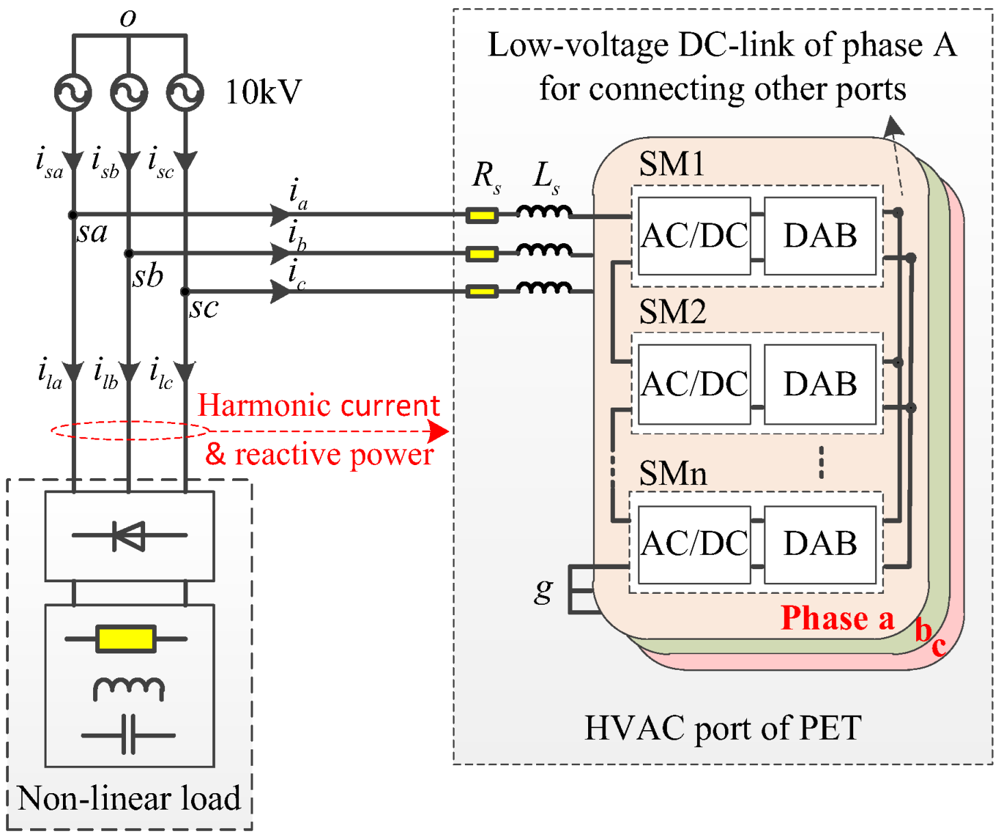
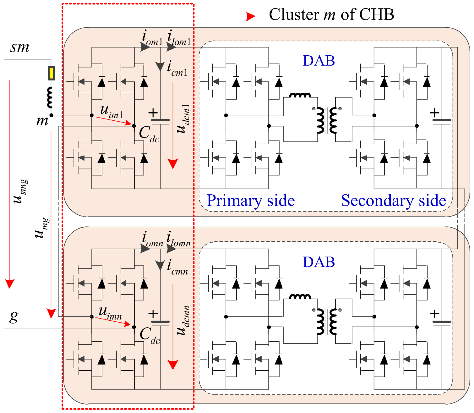
1. Introduction
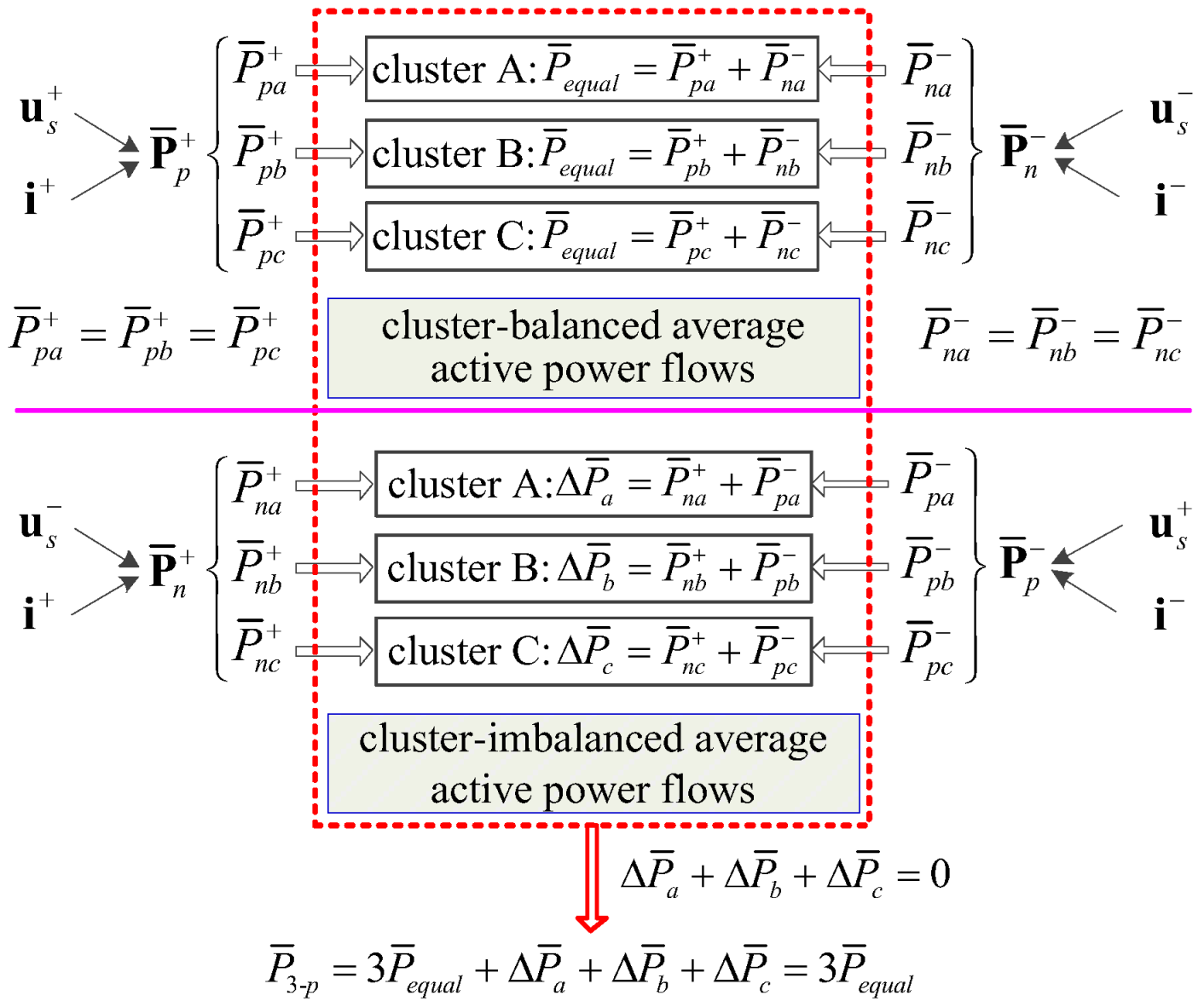
2. Decoupling Principle of Active Power Under Imbalance Operation
3. Average Power Control Strategy
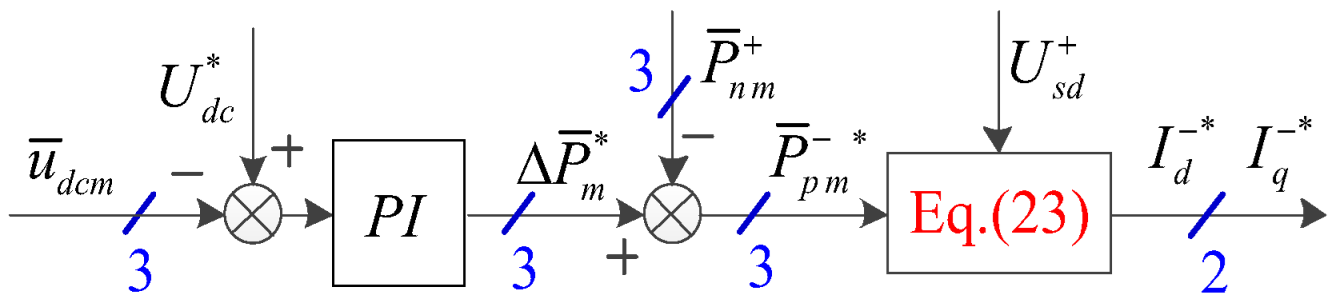
3.1. Stability Control for the Sum of Cluster Average Active Power Flows
3.2. Individual Control for the Cluster Average Active Power Flows
3.3. Reactive Power Compensation Control
4. Decoupling Principle of Voltage and Current Under Distorted Conditions
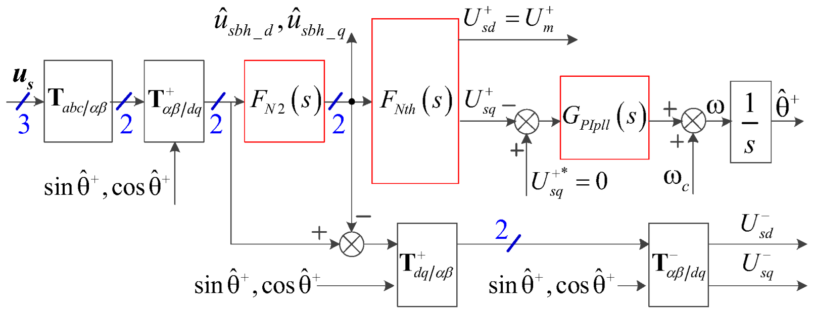
4.1. Voltage Decoupling Principle and the Implementation of SRF-PLL
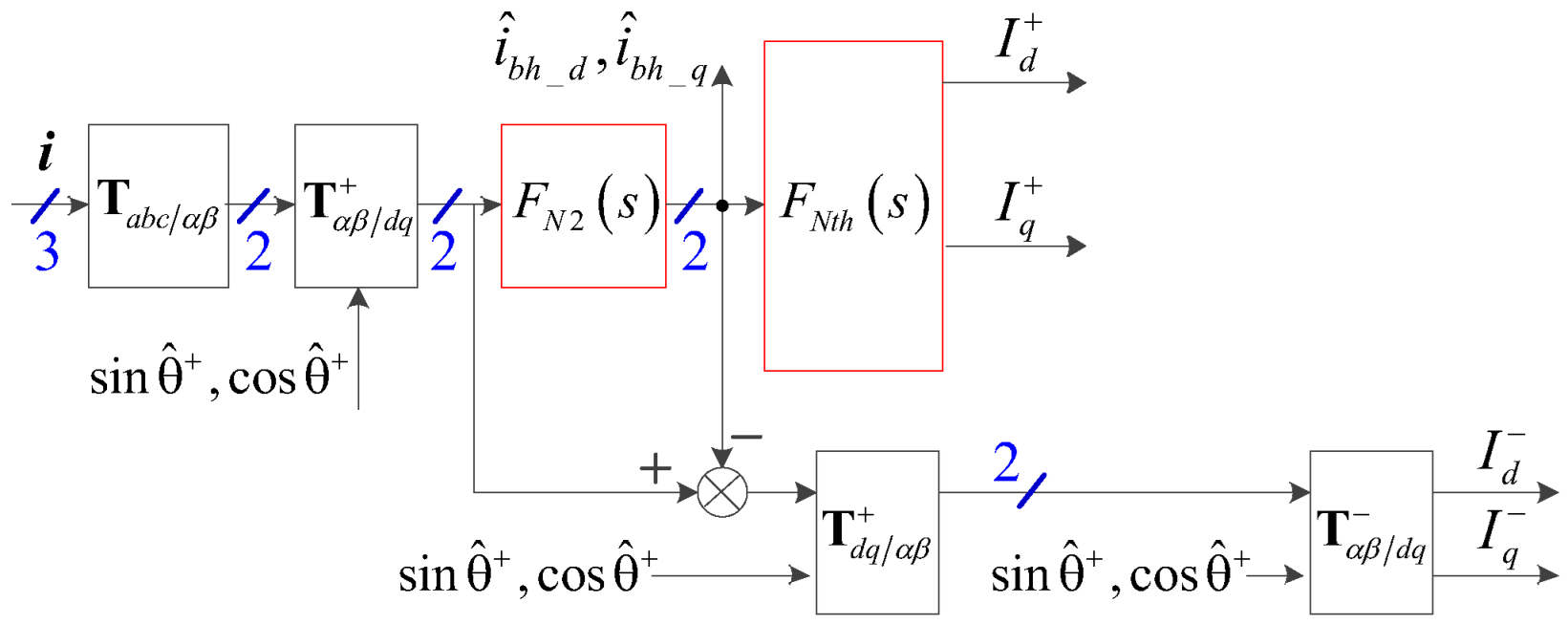
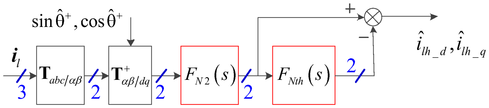
4.2. Current Decoupling Principle
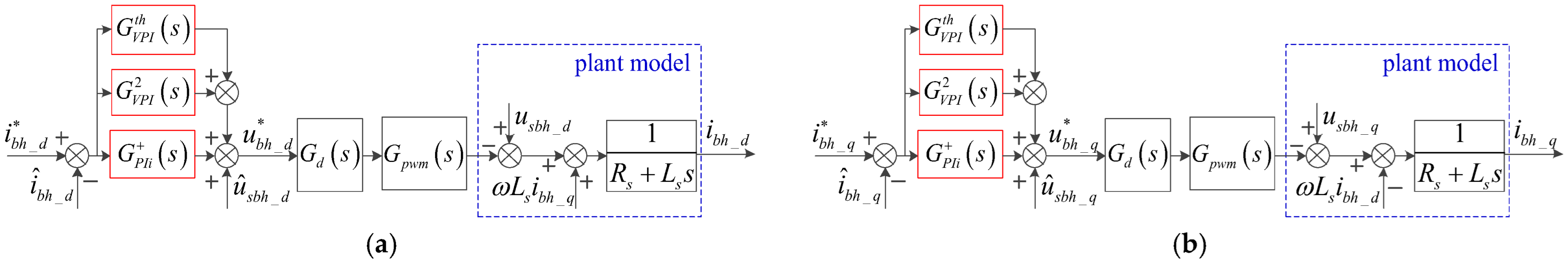
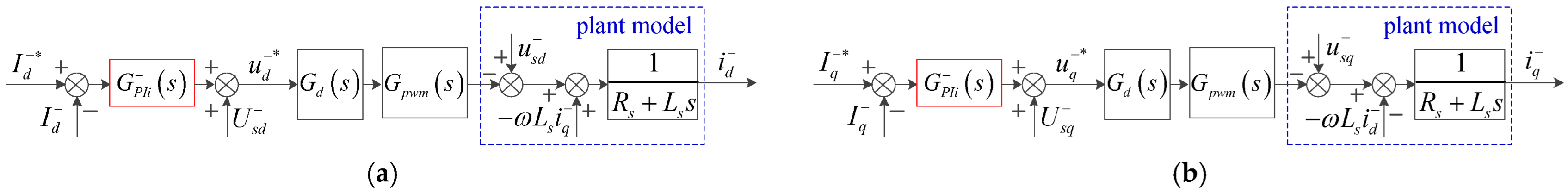
5. Current Control Strategy
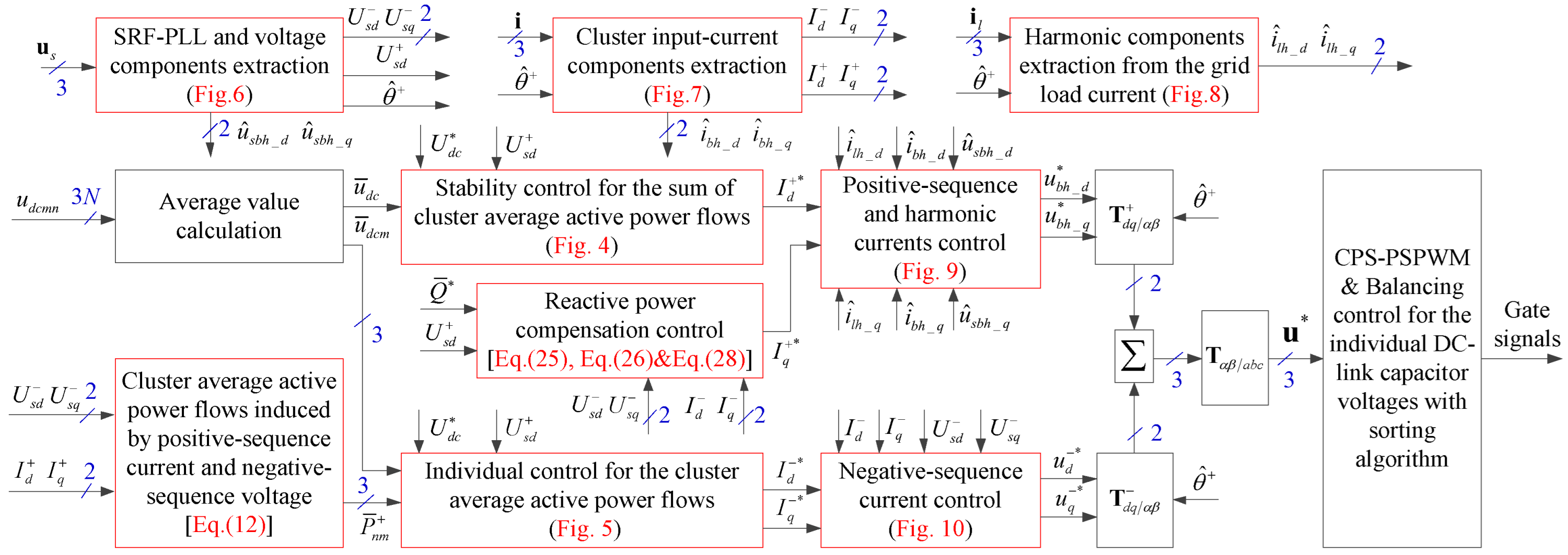
6. The Overall Control Scheme
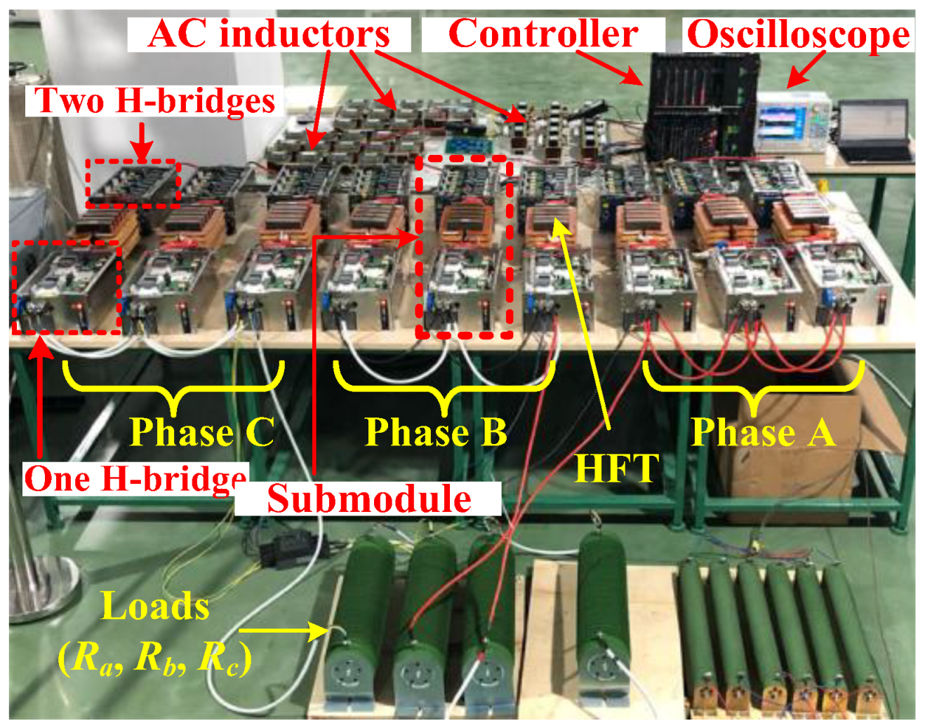
7. Results
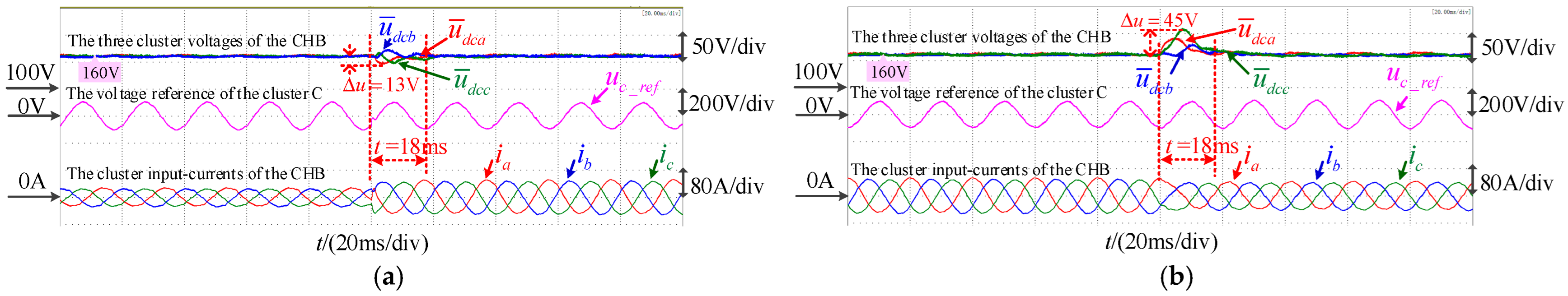
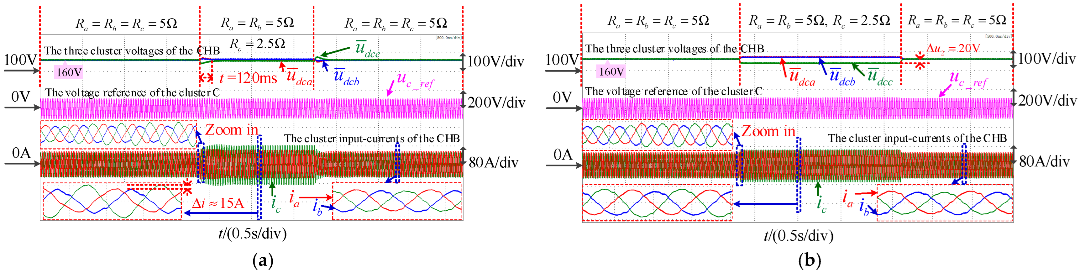
7.1. Experiments for Reactive Power Injection and Cluster Voltage Balancing Control
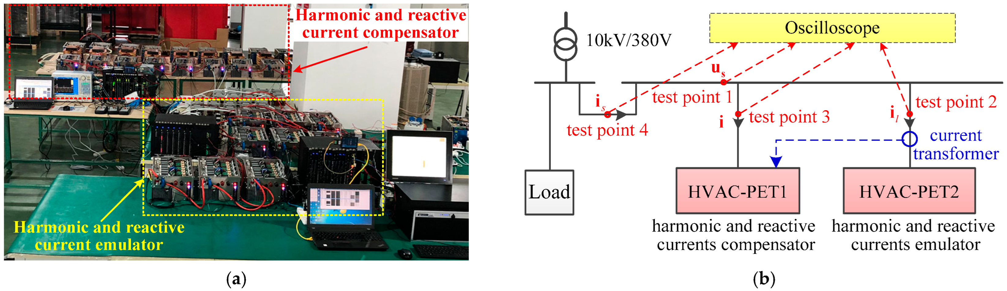
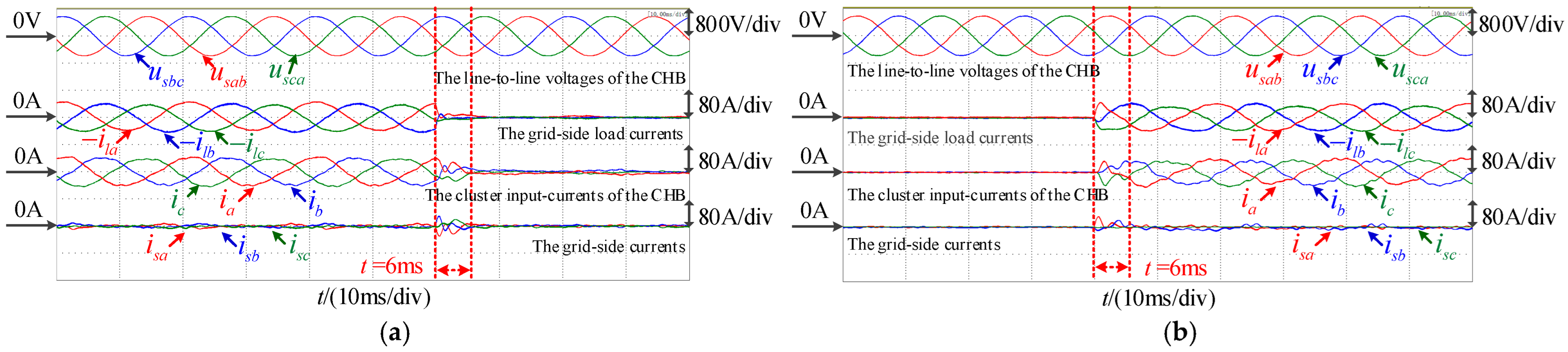
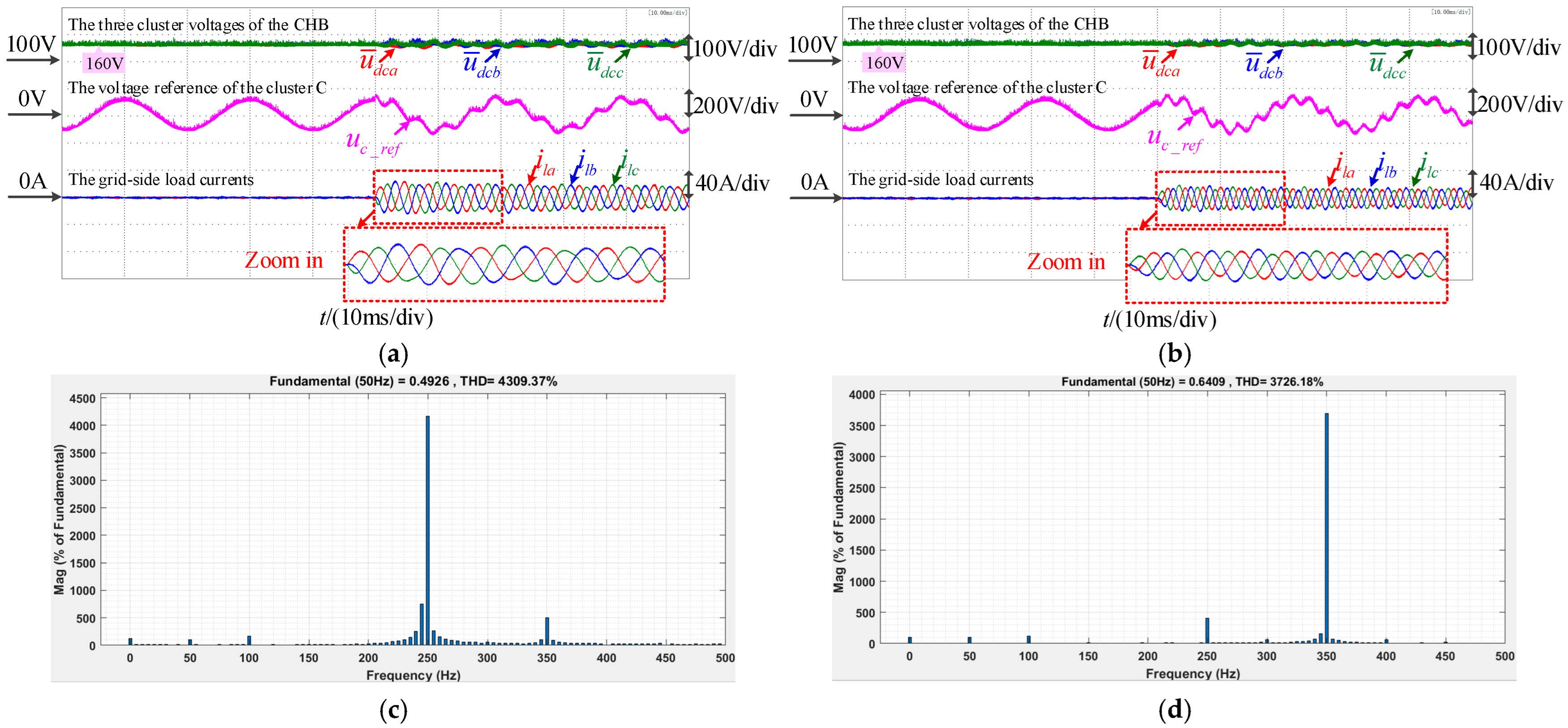
7.2. Experiments for Reactive Power Compensation and Active Power Filtering
8. Conclusions
Author Contributions
Funding
Data Availability Statement
Conflicts of Interest
References
- Shi, Y.; Zhang, X.; Wu, Y.; Li, W.; Qi, L. Application Expansion of DC Bias Suppression for Hybrid Transformers in Flexible AC Grid Regulation. IEEE Trans. Power Electron. 2024, 39, 15398–15402. [Google Scholar] [CrossRef]
- Li, K.; Wen, W.; Zhao, Z.; Yuan, L.; Cai, W.; Mo, X.; Gao, C. Design and Implementation of Four-Port Megawatt-Level High-Frequency-Bus Based Power Electronic Transformer. IEEE Trans. Power Electron. 2021, 36, 6429–6442. [Google Scholar] [CrossRef]
- Chen, Y.; He, J.; Pan, Y.; Liu, R.; Wang, R.; Liu, Z.; Zeng, W.; Sun, M. A Simple Online Fault Location and Tolerant Control Strategy for Power Electronic Transformers with a Single IGBT Open-Circuit Fault. IEEE Trans. Power Electron. 2024, 39, 5522–5535. [Google Scholar] [CrossRef]
- Su, J.; Li, K.; Xing, C. Plug-and-Play of Grid-Forming Units in DC Microgrids Assisted with Power Buffers. IEEE Trans. Smart Grid 2024, 15, 1213–1226. [Google Scholar] [CrossRef]
- Huber, J.E.; Kolar, J.W. Applicability of Solid-State Transformers in Today’s and Future Distribution Grids. IEEE Trans. Smart Grid 2019, 10, 317–326. [Google Scholar] [CrossRef]
- Patel, H.; Hatua, K.; Bhattacharya, S. Hybrid Modulation Technique of MV Grid-Connected Cascaded H-Bridge-Based Power Electronic Transformer Technology. IEEE J. Emerg. Sel. Top. Power Electron. 2025, 13, 2864–2878. [Google Scholar] [CrossRef]
- He, Y.; Yao, C.; Wang, X.; Hu, J. Novel High-Frequency Pulse Permutation Scheme for DC-Link Voltage Balance of CHB-Based PV Solid-State Transformer. IEEE Trans. Power Electron. 2024, 39, 14181–14191. [Google Scholar] [CrossRef]
- Li, Z.; Pei, Y.; Liu, J.; Wang, L.; Leng, Z. Design and Optimization of the MMC-Based Power Electronic Transformer Considering Ripple Power Transfer. IEEE Trans. Power Electron. 2025, 40, 5352–5370. [Google Scholar] [CrossRef]
- Vipin, V.N.; Mohan, N. Sensitivity Analysis of the High-Frequency-Link MMC to DC Link Voltage Ripples in a Back-to-Back Connected MMC-Based Power Electronic Transformer. IEEE Trans. Power Electron. 2025, 40, 8691–8708. [Google Scholar] [CrossRef]
- Li, J.; Chen, J.; Gong, C. An Optimized Reactive Power Compensation Strategy to Extend the Working Range of CHB Multilevel Grid-Tied Inverters. IEEE Trans. Power Electron. 2023, 38, 5500–5512. [Google Scholar] [CrossRef]
- Wen, W.; Zhao, Z.; Ji, S.; Yuan, L. Low-voltage ride through of multi-port power electronic transformer. iEnergy 2022, 1, 243–256. [Google Scholar] [CrossRef]
- Xu, Y.; Tolbert, L.M.; Chiasson, J.N.; Campbell, J.B.; Peng, F.Z. A generalised instantaneous non-active power theory for STATCOM. IET Electr. Power Appl. 2007, 1, 853–861. [Google Scholar] [CrossRef]
- Xu, Y.; Tolbert, L.M.; Kueck, J.D.; Rizy, D.T. Voltage and cur-rent unbalance compensation using a static var compensator. IET Power Electron. 2010, 3, 977–988. [Google Scholar] [CrossRef]
- Song, Q.; Liu, W.H. Control of a cascade STATCOM with star configuration under unbalanced conditions. IEEE Trans. Power Electron. 2009, 24, 45–58. [Google Scholar] [CrossRef]
- Lu, D.; Wei, M.; Wu, T.; Hu, H. Extension of Negative-Sequence Current Compensation Range Based on Negative- and Zero-Sequence Voltage Injection for Hybrid Cascaded STATCOM. IEEE Trans. Ind. Electron. 2024, 71, 4340–4352. [Google Scholar] [CrossRef]
- Wang, D.; Tian, J.; Mao, C.X.; Lu, J.M.; Duan, Y.P.; Qiu, J.; Cai, H.H. A 10kV/400V 500kVA electronic power transformer. IEEE Trans. Ind. Electron. 2016, 63, 6653–6663. [Google Scholar] [CrossRef]
- Santiprapan, P.; Areerak, K.; Areerak, K. An Adaptive Gain of Proportional-Resonant Controller for an Active Power Filter. IEEE Trans. Power Electron. 2024, 39, 1433–1446. [Google Scholar] [CrossRef]
- Yepes, A.G.; Freijedo, F.D.; Doval-Gandoy, J.; López, Ó.; Malvar, J.; Fernandez-Comesaña, P. Effects of Discretization Methods on the Performance of Resonant Controllers. IEEE Trans. Power Electron. 2010, 25, 1692–1712. [Google Scholar] [CrossRef]
- Zheng, L.; Geng, H.; Yang, G. Fast and Robust Phase Estimation Algorithm for Heavily Distorted Grid Conditions. IEEE Trans. Ind. Electron. 2016, 63, 6845–6855. [Google Scholar] [CrossRef]
- Wu, T.-F.; Hsieh, H.-C.; Hsu, C.-W.; Chang, Y.-R. Three-Phase Three-Wire Active Power Filter with D-Σ Digital Control to Accommodate Filter-Inductance Variation. IEEE J. Emerg. Sel. Top. Power Electron. 2016, 4, 44–53. [Google Scholar] [CrossRef]
- Qasim, M.; Kanjiya, P.; Khadkikar, V. Artificial-Neural-Network-Based Phase-Locking Scheme for Active Power Filters. IEEE Trans. Ind. Electron. 2014, 61, 3857–3866. [Google Scholar] [CrossRef]
- Wen, W.; Li, K.; Zhao, Z.; Yuan, L.; Mo, X.; Cai, W. Analysis and Control of a Four-Port Megawatt-Level High-Frequency-Bus-Based Power Electronic Transformer. IEEE Trans. Power Electron. 2021, 36, 13080–13095. [Google Scholar] [CrossRef]


| Variable | Symbol | Value |
|---|---|---|
| Cascaded submodule number | N | 3 |
| AC filter inductor | Ls, Rs | 2.8 mH, 28 mΩ |
| DC-link capacitor | Cdc | 1 mF |
| HFT ratio | n1:n2 | 1:1 |
| Line-to-line rms voltage of PCC | Us | 380 V |
| Nominal DC voltage of submodule | 160 V | |
| Switching frequency | fsw | 20 kHz |
| Sampling frequency | fs | 10 kHz |
| Variable | Symbol | Value |
|---|---|---|
| Coefficients of notch filter FN2 | Q, ωb | 250.0, 80 Hz |
| Coefficients of notch filter FN6 | Q, ωb | 250.0, 80 Hz |
| Coefficients of notch filter FN12 | Q, ωb | 250.0, 80 Hz |
| PI regulator for PLL | kPpll, TIpll | 2.0, 0.07 |
| PI regulator for ibh | 1.5, 0.1 | |
| PI regulator for i− | 1.5, 0.1 | |
| Coefficients of VPI controller | kP2, kR2 | 0.05, 0.5 |
| Coefficients of VPI controller | kP6, kR6 | 0.05, 0.5 |
| Coefficients of VPI controller | kP12, kR12 | 0.05, 0.5 |
| PI regulator for average cluster voltage | kPacv, TIacv | 0.8, 0.016 |
| PI regulator for cluster voltage | kPcv, TIcv | 10.0, 0.5 |
Disclaimer/Publisher’s Note: The statements, opinions and data contained in all publications are solely those of the individual author(s) and contributor(s) and not of MDPI and/or the editor(s). MDPI and/or the editor(s) disclaim responsibility for any injury to people or property resulting from any ideas, methods, instructions or products referred to in the content. |
© 2025 by the authors. Licensee MDPI, Basel, Switzerland. This article is an open access article distributed under the terms and conditions of the Creative Commons Attribution (CC BY) license (https://creativecommons.org/licenses/by/4.0/).
Share and Cite
Wen, W.; Zhan, T.; Zhang, Y.; Nie, J. Decoupling Control for the HVAC Port of Power Electronic Transformer. Energies 2025, 18, 4131. https://doi.org/10.3390/en18154131
Wen W, Zhan T, Zhang Y, Nie J. Decoupling Control for the HVAC Port of Power Electronic Transformer. Energies. 2025; 18(15):4131. https://doi.org/10.3390/en18154131
Chicago/Turabian StyleWen, Wusong, Tianwen Zhan, Yingchao Zhang, and Jintong Nie. 2025. "Decoupling Control for the HVAC Port of Power Electronic Transformer" Energies 18, no. 15: 4131. https://doi.org/10.3390/en18154131
APA StyleWen, W., Zhan, T., Zhang, Y., & Nie, J. (2025). Decoupling Control for the HVAC Port of Power Electronic Transformer. Energies, 18(15), 4131. https://doi.org/10.3390/en18154131