A Comparative Study of Statistical and Machine Learning Methods for Solar Irradiance Forecasting Using the Folsom PLC Dataset

Abstract

The increasing penetration of photovoltaic solar energy has intensified the need for accurate production forecasting to ensure efficient grid operation. This study presents a critical comparison of traditional statistical methods and machine learning approaches for forecasting solar irradiance using the benchmark Folsom PLC dataset. Two primary research questions are addressed: whether machine learning models outperform traditional techniques, and whether time series modelling improves prediction accuracy. The analysis includes an evaluation of a range of models, including statistical regressions (OLS, LASSO, ridge), regression trees, neural networks, LSTM, and random forests, which are applied to physical modelling and time series approaches. The results reveal that although machine learning methods can outperform statistical models, particularly with the inclusion of exogenous weather features, they are not universally superior across all forecasting horizons. Furthermore, pure time series approach models yield lower performance. However, a hybrid approach in which physical models are integrated with machine learning demonstrates significantly improved accuracy. These findings highlight the value of hybrid models for photovoltaic forecasting and suggest strategic directions for operational implementation.

1. Introduction

Production management in modern electrical systems is one of the fundamental pillars supporting the stability, efficiency, and sustainability of the energy supply. In this context, system reliability and cost minimisation are the primary goals. One of the main operational challenges involves maintaining a dynamic balance between electricity demand and available generation in real time. Since electricity is not easily storable, a precise balance between production and service is essential to avoid both energy waste and the risk of blackouts or grid overloads [1].

The increasing integration of renewable energy sources, especially intermittent ones such as photovoltaic (PV) solar and wind, has profoundly transformed the structure and dynamics of electrical systems. Whereas traditional sources such as thermal, nuclear, and even hydroelectric plants allow for highly controlled production management, newer renewable plants depend heavily on weather conditions and are generally more volatile [2]. However, the current regulations in many countries give dispatch priority to renewables, forcing their use over more controllable sources, and although this may be environmentally beneficial, it introduces significant complexity into the operation of the system [3].

Photovoltaic solar energy, in particular, has undergone exponential growth in recent years. As of 2024, the global installed solar capacity exceeded 1400 GW, with annual production reaching 2000 TWh, representing about 7% of global electricity generation [4]. This growth has been driven by technological cost reductions, incentive policies, and increasing environmental awareness.

Production forecasting has become a central aspect of management. Planning and scheduling of production units are conducted based on demand forecasting, and effective management of this new energy reality also requires the forecasting of renewable energy production. While traditional models have relied on statistical techniques, machine learning (ML) approaches have gained in importance in recent years, as these algorithms have shown a superior ability to capture non-linear patterns and adapt to highly variable contexts.

This article presents a critical review of the primary forecasting methods applied to electricity production management, with a special focus on ML models. The objective is to enable the development and selection of models that can respond effectively and reliably in real time to the requirements of a prediction system embedded in a future home energy management system. The performance of these methods is evaluated based on the Folsom photovoltaic plant dataset that has been widely used in the scientific literature [5]. This facility has become a benchmark for the validation of predictive models due to the availability and quality of its data. Two research questions are addressed in the article:

• RQ1: Are ML methods more accurate than traditional methods?
• RQ2: Can the use of time series enhance forecast accuracy?

The remainder of this paper is structured as follows: Section 2 presents a literature review related to the main topic, and Section 3 explains the methods and materials used for the study. Section 4 presents the results, while Section 5 concludes the article.

2. Related Literature

The reliability of PV production forecasting is essential for proper functioning of the power system. The forecasting horizons used for solar and wind power prediction can vary significantly—from very short-term (minutes to one hour) to long-term (months to years), depending on the intended application [6]. This review primarily focuses on short-term forecasting, which is critical for operational decision-making and grid stability.

Forecasting errors in Europe range between 15% and 100%, measured as a normalised root mean square error (RMSE) relative to the mean [7]. A significant proportion of this error is influenced by weather conditions, which can introduce an RMSE up to 35% in a prediction [8]. This forecasting error propagates from generation to the grid, which is operated by a transmission system operator (TSO) or an independent system operator (ISO), with an ultimate impact on the distribution networks. Although the economic cost of this error is difficult to generalise, it is estimated as ranging between 40 and 140 USD/MWh [9]. With the substantial increase in PV generation currently under way, this impact is likely to grow, and there is consequently a growing interest in improving forecasting accuracy [10].

The most fundamental element of a forecast is solar irradiance. In general, two distinct methodological approaches are employed, based on time series data or on physical models [11]. These approaches differ in conceptual terms, regardless of whether statistical or ML techniques are used for the modelling process. For forecasting based on physical models, the irradiance is initially estimated under favourable weather conditions, known as clear-sky conditions. These models use cell temperature to calculate power output. Notable examples include the nominal operating cell temperature (NOCT) models [12] and the Sandia models [13], developed by Sandia National Laboratories; comparative studies indicate minimal differences in performance between these approaches [14]. These models are subsequently adjusted using meteorological data, so that the final irradiance estimate accounts for cloud cover, wind, and other atmospheric conditions [15]. In this context, the integration of satellite imagery with radiative transfer physical models to estimate surface solar irradiance at high spatial and temporal resolution has given improved results [16]. SoDa (solar radiation data) is a platform that provides access to solar irradiance databases and estimation models, such as HelioClim and the Heliosat-2 model, developed by MINES ParisTech [17].

Forecasting using statistical and time series models is carried out to estimate direct irradiance, and to predict the meteorological parameters that influence irradiance, thereby complementing physical models [18]. Classical time series methods are common: for example, Singh and Garg [19] and Sapundzhi et al. [20] have employed ARIMA-based models, although hybrid models incorporating ML are generally preferred. Despotovic et al. [21] used autoregressive models with transfer learning to forecast PV output in Spain. Torres et al. [22] developed a deep learning-based solar power forecasting system in which multiple data sources were integrated (meteorological, historical production, satellite, etc.). Their model combined convolutional neural networks (CNNs) to extract the spatial features from meteorological data with long short-term memory (LSTM) networks to capture temporal dynamics and found that this approach significantly enhanced predictive performance compared to traditional models, even when applied to large datasets [23]. This method was also applied by Qing and Niu to Cape Verde datasets [24]. Xu et al. [25] presented a hybrid short-term PV output forecasting approach in which signal decomposition was combined with the XGBoost (Extreme Gradient Boosting) model.

The use of satellite imagery in forecasting is playing an increasingly important role. The application of cross-correlation techniques to cloud features in sky images has enabled minute-scale irradiance forecasts, with a forecasting RMSE of 17% having been achieved for the global horizontal irradiance (GHI) for partly cloudy skies [26]. The introduction of a three-dimensional CNN (3D-CNN) architecture for extracting spatiotemporal features from video-like sky image sequences enabled their model to significant outperform traditional two-dimensional CNN (2D-CNNs) and LSTM-based hybrid models in the prediction of GHI [27]. Bu et al. [28] combined a spatiotemporal analysis of satellite images interpreted through CNN and LSTM networks to simulate the impact of cloud cover on irradiance. Similarly, the PV2-state model was enhanced using all-sky images to estimate sunshine indices and forecast photovoltaic output, achieving improved skill scores for 15 to 30 min intervals [29].

In order to promote research in this field, several noteworthy initiatives have been undertaken to enable solar production data to be openly shared [30,31]. As the integration of PV systems into electric grids progresses, it is becoming essential to improve forecasting methods. Sengupta et al. [32] have compiled and made available a comprehensive dataset of solar irradiance and meteorological parameters across the United States that spanned the last 30 years. One critical aspect of any dataset is its reliability. Vignola et al. [33] emphasised the need for ground-based measurements over a period of at least one to two years in order to ensure data quality and representativeness. A good example is offered by the dataset released by Pedro et al. [5], which is commonly referred to as the PLC dataset. This dataset is widely used for benchmarking forecasting models [34].

An understanding of the outcomes of previously developed models is a necessary starting point for evaluating the effectiveness of the forecasting approaches proposed in this study and for framing a meaningful comparison of their performance. Marinho et al. [35] explored the issue of short-term solar irradiance forecasting using deep learning techniques (CNN-1D, LSTM, and CNN-LSTM) applied to the Folsom (USA) dataset. The forecasting error, evaluated using the RMSE, was approximately 75 W/m² for GHI. Oliveira et al. [36] developed a novel architecture and used the Folsom data for benchmarking. Using XGBoost, their model achieved an average RMSE of 39 W/m² for intra-hour GHI forecasting and 48.5 W/m² for intra-day GHI forecasting. However, for direct normal irradiance (DNI) prediction, the RMSE values were significantly higher, with values of 86.8 W/m² for intra-hour and 109.9 W/m² for intra-day forecasts. Alternative techniques such as support vector regression (SVR), group method of data handling (GMDH), and quantum neural networks (QNN) yielded RMSE levels that were approximately 25% to 50% higher, a finding that underscored the relative effectiveness of the XGBoost approach [36]. Zhang et al. [37] conducted a comparative evaluation of seven forecasting architectures tailored for ultra-short-term solar irradiance prediction, with lead times of 2, 6, and 10 min. These models included a baseline statistical persistence model (SPM), an AutoML-based model (NUM) based on meteorological inputs, and five deep learning architectures combining spatial and temporal features based on CNN and ViT methods. The average RMSE for GHI forecasting was approximately 95 W/m².

Yang et al. [38] compared models such as quantile regression forests, Gaussian process regression (GPR), Bayesian model averaging (BMA), ensemble model output statistics (EMOS), and persistence-based probabilistic models, also using the same dataset [39].

Table 1. Summary of recent methods for solar irradiance forecasting using the Folsom dataset and similar benchmarks.

Reference	Authors	Methods Used	Forecast Horizon	Reported Results
[19]	Singh & Garg	ARIMA and S-ARIMA	Short-term on Power Production	nRMSE 3.4% on a 24 MW power station
[21]	Despotovic et al.	Autoregressive + Transfer Learning for Spanish PV	Short-term	nRMSE ≈ 19% for 30 min, 31% for 180 min and 34% for 6h for GHI
[22,23]	Torres et al.	CNN + LSTM with meteorological, historical, and satellite data for Queensland (AUS)	Short-term (intra-day)	RMSE ≈ 148 MW for PV power in a 70 MW PV plant
[24]	Qing & Niu	LSTM + weather forecasts for Cape Verde	Day-ahead (hourly)	RMSE ≈ 76 W/m2 for GHI
[25]	Xu et al.	Signal decomposition + XGBoost	Short-term	eRMSE ≈ 1.19 for Power (MW)
[26]	Alonso-Montesinos et al.	Sky images + cloud cross-correlation	Minute-level	RMSE ≈ 17% for GHI under partly cloudy conditions
[27]	Zhao et al.	3D-CNN vs. 2D-CNN and LSTM	Short-term (DNI)	nRMSE ≈ 30% for DNI
[28]	Bu et al.	CNN + LSTM on satellite images for several PV Stations in China	Short-term	RMSE ≈ 60–80 W/m2
[29]	Paulescu et al.	PV2-state + sky imagery	Intra-hour (15–30 min)	nRMSE ≈ 23%
[35]	Marinho et al.	CNN-1D, LSTM, CNN-LSTM	Short-term	RMSE ≈ 75 W/m2 (GHI, Folsom dataset)
[36]	Oliveira et al.	XGBoost, SVR, GMDH, QNN	Intra-hour and intra-day	RMSE for GHI: 39–48.5 W/m2 for DNI: 86.8–109.9 W/m2
[37]	Zhang et al.	AutoML, CNN, ViT, SPM	Ultra short-term (2, 6, 10 min)	RMSE for GHI ≈ 95 W/m2

summarises the main forecasting methods and results reported in the reviewed literature, highlighting the diversity of approaches, prediction horizons, and accuracy levels achieved across studies.

3. Materials and Methods

3.1. Dataset

In this study, we use a dataset that is freely available from the Zenodo repository under the https://doi.org/10.5281/zenodo.2826939, commonly called the Folsom PLC dataset. This was created by Pedro et al. [5] and contains detailed measurements from the California Independent System Operator (CAISO) headquarters located in Folsom, CA, USA. The data include single-minute frequency recordings of GHI and DNI, as well as information on several weather conditions such as the ambient temperature, relative humidity, wind speed and direction, pressure, etc. In addition to on-site measurements, the dataset also includes meteorological forecast variables obtained from the North American Mesoscale Forecast System (NAM), sky images, and satellite images.

The primary reason for selecting this dataset was its extensive use in the scientific community. The Folsom PV dataset has been widely studied in the context of PV power forecasting and has served as a benchmark in numerous research articles. Its frequent use in the literature means that consistent comparisons can be made across different predictive modelling approaches, thereby facilitating an objective evaluation of the performance of a model. Moreover, its public availability and data quality make it particularly suitable for reproducible and comparative research.

Several authors have utilised this dataset to assess and benchmark solar forecasting approaches; for example, it has served as the basis for evaluating probabilistic forecasting methods using ensemble and hybrid models [38,39], as well as for the implementation of deep learning and QNNs for solar irradiance prediction [36].

3.2. Machine Learning Methods

In this study, we considered all ML methods that were capable of providing regression-based predictions, although only those that yielded the best results are presented here. We present a brief description of each model below.

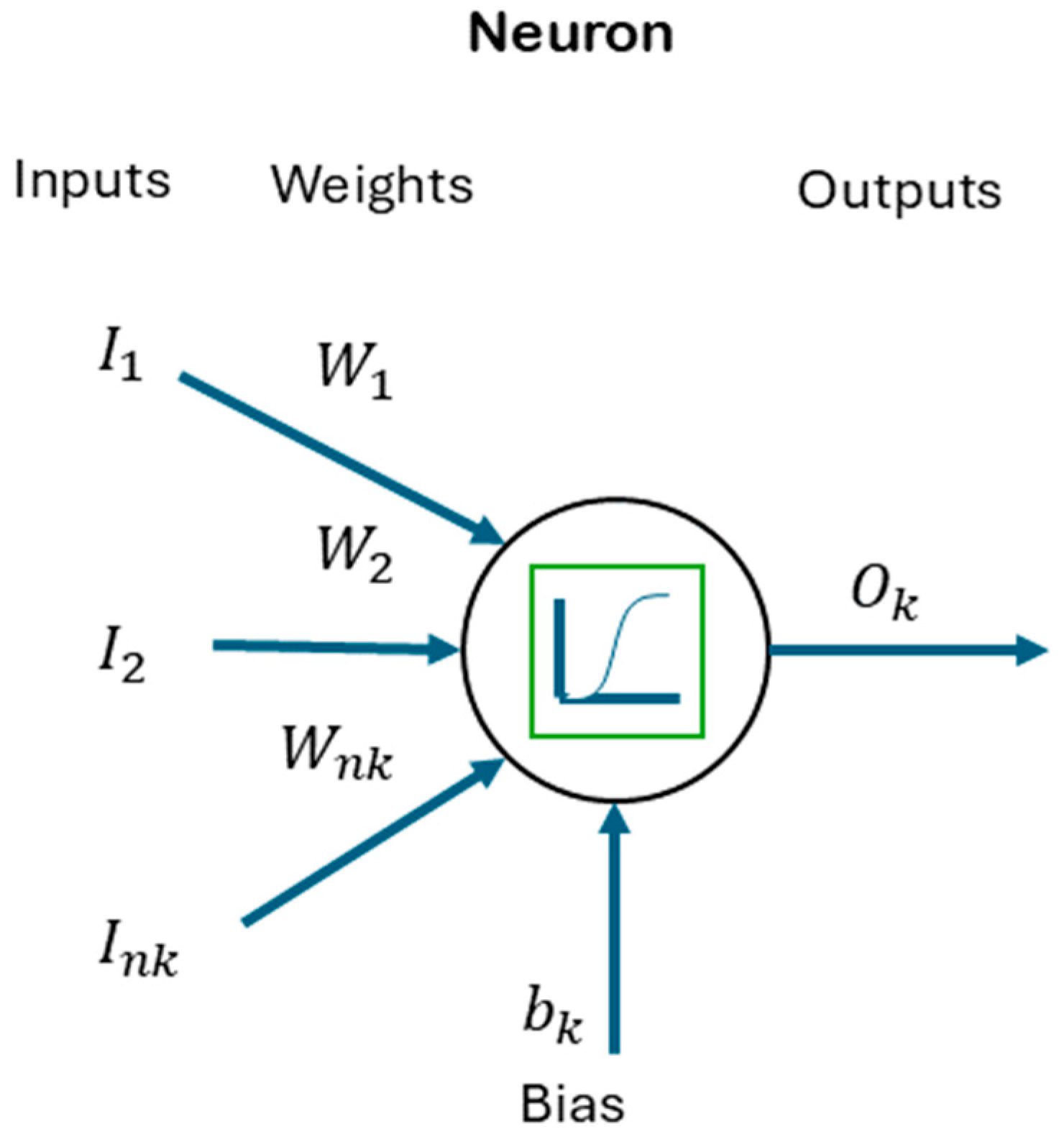
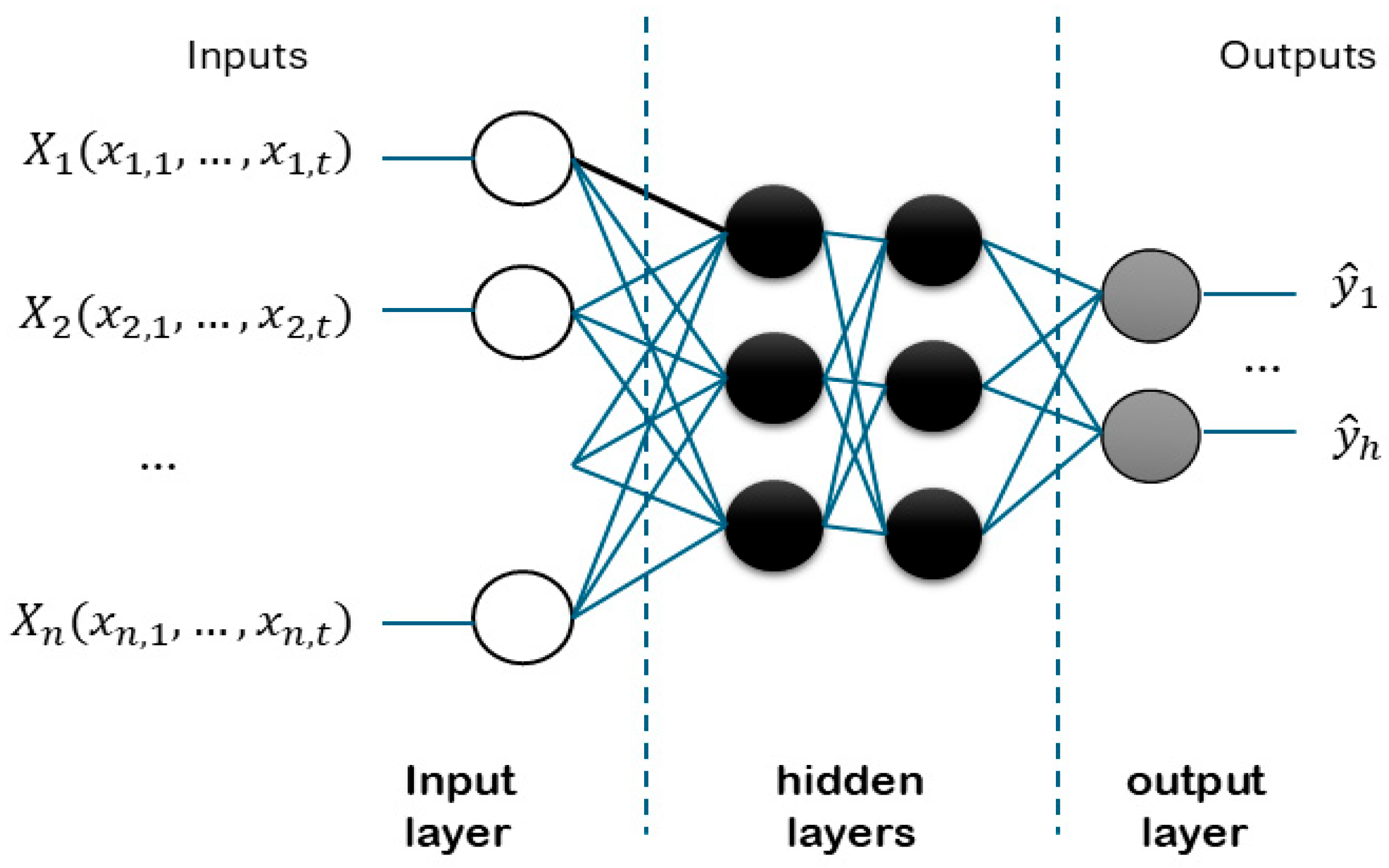
3.2.1. Neural Networks

Neural network (NN) models are based on computational models formed by interconnected functional nodes called neurons [40]. Figure 1 shows a neuron of the network in detail. Each neuron produces an output signal ($O_k$) by processing input signals using ($I_i$) through an activation function ($f$).

Each neuron ($k$) is connected via links ($w_i$) called axons, which assign weights to the input received by the neuron. Biases ($b_k$) are also added to increase the flexibility of the model. Each neuron is connected to several input signals ($n_k$) which may be outputs from other neurons, or the predictor variables.

The activation function introduces non-linearity and may be a linear, sigmoid, tanh, ReLU function, etc., depending on the purpose of the network. The output of a neuron is calculated as shown in (1).

$$O_k=\sum _{i=1}^{n_k}{w}_i{I}_i+b_k$$

(1)

Neurons are organised into layers called the input, hidden, and output layers, as shown in Figure 2. A common type is a feedforward neural network, which consists of one input layer, one or more hidden layers, and one output layer. It can be seen that the input variables (predictors, $X_n$) are linked to the neurons lying in the input layer, which must all have the same number of observations $t$. The data may either be endogenous or exogenous. The neurons in the output layer provide forecasts of the output variable $\widehat{y}$ for $h$ steps ahead. The general formulation is shown in (2):

$$\widehat{y}=f(X_1,X_2,\dots ,X_n)$$

(2)

Training involves adjusting the weights to minimise the difference between the predicted and actual values, typically using gradient descent and a loss function such as the mean squared error (MSE).

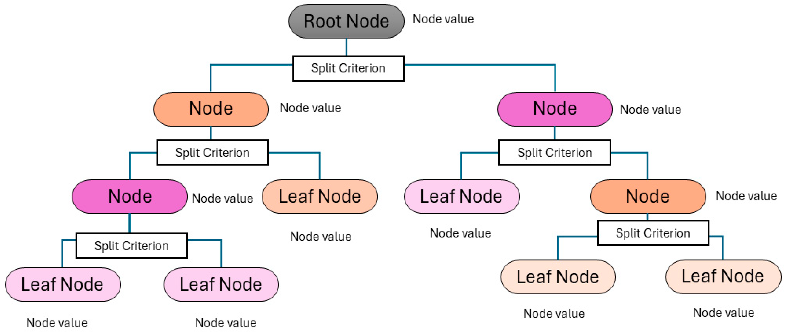
3.2.2. Regression Trees

A regression tree (RT) is a specific version of the decision tree (DT) algorithm [41] and predicts values by recursively partitioning the data based on predictor variables, in the same way as in regression. The way in which the information is graphed is similar to a tree, as each node is split into branches until a terminal node (leaf) containing the response value is reached. Figure 3 shows a generic representation of the tree.

Starting from the root node, a decision is made at each internal node $j$ as to which path to follow, based on the splitting criterion defined at that node, which determines the behaviour of the branch from that point onward, called the region ($R_j$). This process is repeated until the leaf nodes at the bottom of the tree are reached. Given a dataset $\left(X,y\right) = \left(X_1,X_2,\dots ,X_n,y\right)$, and depending on the splitting criteria, a leaf node $j$ is reached from which the value $y_j$ is obtained as the node value. The value at each internal node (${\widehat{y}}_{R_j}$) is computed as the weighted average of the values of the branches (regions also known as rectangles) downstream from that node.

To construct the tree structure and determine the splitting criteria, algorithms rely on computation of the error through specific metrics, with the most common one for regression being CART (classification and regression trees). The process of constructing an RT involves determining the optimal number of terminal nodes,$T$, as well as selecting a suitable regularisation paramete $\alpha$ to find a trade-off between the complexity of the model and data fitting. A larger number of nodes typically allows the model to capture more intricate patterns in the data, but it also increases the risk of overfitting. Conversely, a smaller tree may generalise better but at the cost of reduced accuracy.

A cost-complexity pruning approach is commonly employed to address this trade-off where the objective is to minimise the function (3).

$$\sum _{j=1}^{\left|T\right|}\sum _{x_i\in R_j}{\left(y_i-{\widehat{y}}_{R_j}\right)}^2+\alpha \left|T\right|$$

(3)

where $\left|T\right|$ is the number of terminal nodes in the tree, and $\alpha$ is a non-negative parameter that penalises the tree complexity. Optimal values of T and α are typically obtained through cross-validation: this involves partitioning the dataset into training and validation subsets, fitting trees with varying complexity, and selecting the configuration that minimises the cross-validated error. This procedure ensures that the final model achieves a good balance between predictive accuracy and generalisation capability.

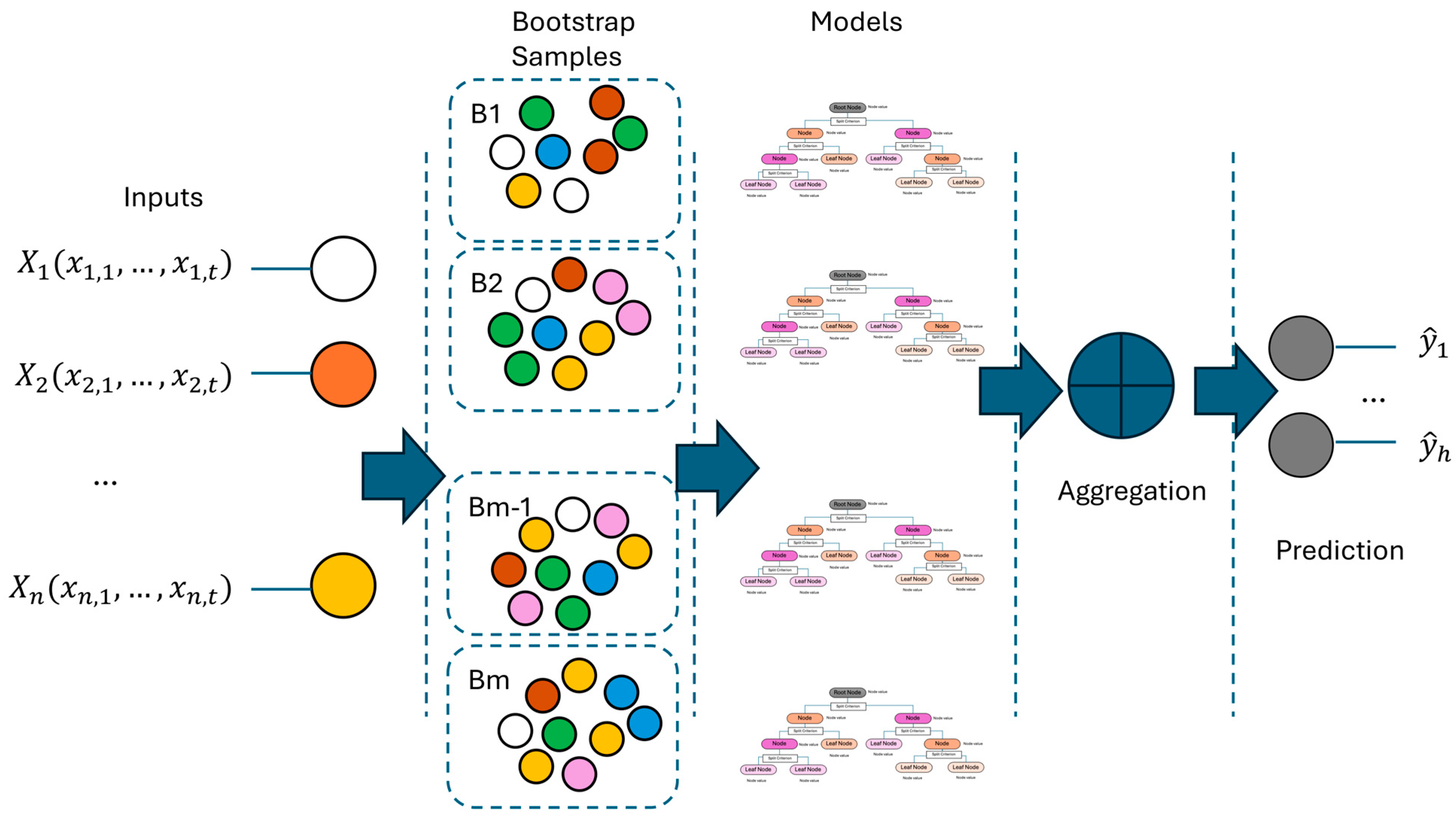
3.2.3. Random Forest Ensemble

A combination of simple processes can yield remarkable results, and this philosophy underpins the development of ensemble methods based on DT. These methods can enhance the prediction accuracy through combining simpler models. Of these, random forest (RF) stands out as a robust technique that has consistently delivered strong performance [42].

Initially, the bagging (bootstrap aggregating) technique is applied, as illustrated in Figure 4. This method involves dividing the dataset into $m$ training subsets $B_i$, on which a series of sampling operations with replacement are performed. Simple models (in this case, RT) are then fitted to each subset. Each sample drawn is independent from the others, which contributes to increasing the variability among the models.

RF is an ensemble of regression trees, each of which is trained on a different bootstrap sample of the original dataset, thereby introducing a layer of randomness. A random subset of features is selected at each split within a tree, from which the best split is chosen. The advantage of this technique lies in its ability to decorrelate the trees, which significantly enhances the generalisation capacity of the ensemble and reduces overfitting.

The final prediction of a regression model based on RF is generally obtained by averaging the outputs of all individual trees. This aggregation smooths out the variance inherent in single DTs, resulting in more stable and accurate predictions.

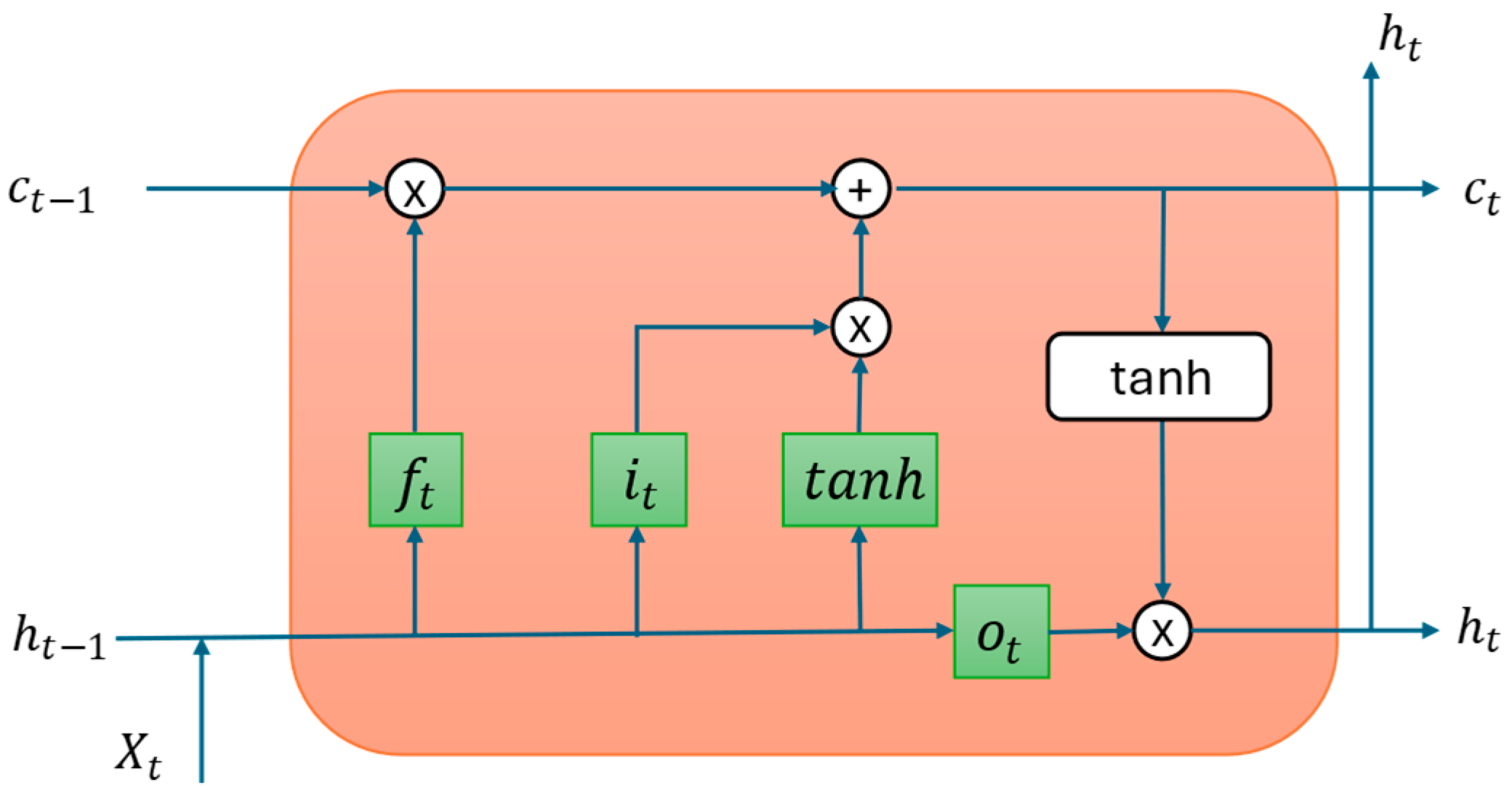
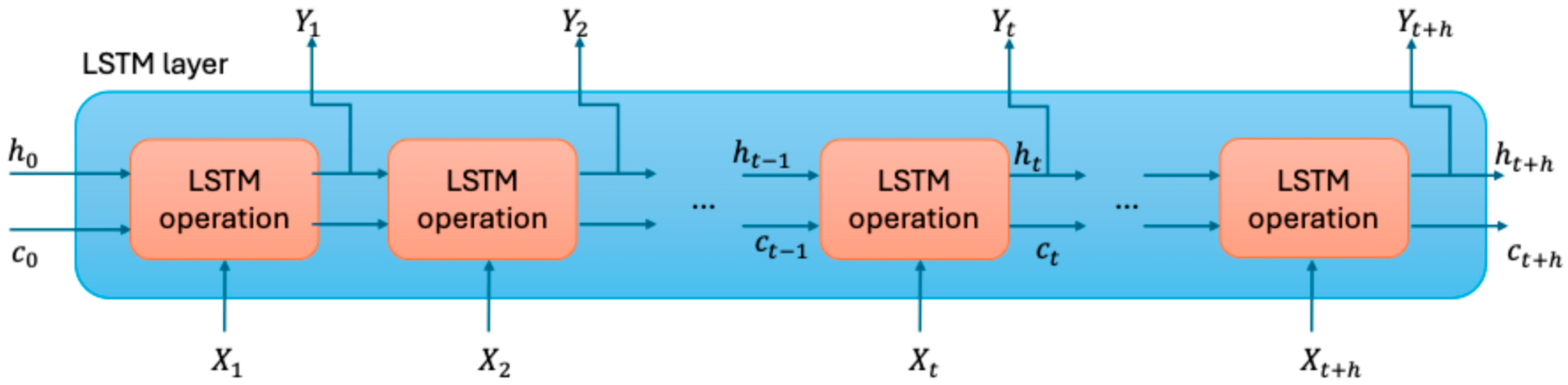
3.2.4. LSTM Networks

A specialised version of a recurrent neural network (RNN) is an LSTM network. This was designed to enable efficient modelling of temporal sequences and time-dependent patterns in order to avoid the problems with the gradient that arise in RNNs during training [43].

An LSTM network is structured in the form of an input neuron layer, an output layer, and one or more hidden layers. These hidden layers are organised into cells as shown in Figure 5. Each cell consists of a series of gates, known as $i_t$ (input), $o_t$ (output), $f_t$ (forget), and state ($c_t$). Each gate has a purpose, such as information added to the input, information about the cell’s state, and information to be removed from the cell, respectively. In addition, through the use of the $\tan \mathrm{h}$ function, the model can incorporate candidate cells to provide information from other cells.

The equations in the compact form are shown in Equations (4)–(9):

$${\mathrm{f}}_{\mathrm{t}}={\sigma }_t(W_f{x}_t+U_f{h}_{t-1}+b_f)$$

(4)

$$i_t={\sigma }_t(W_i{x}_t+U_i{h}_{t-1}+b_i)$$

(5)

$$o_{\mathrm{t}}={\sigma }_t(W_o{x}_t+U_o{h}_{t-1}+b_o)$$

(6)

$${\tilde{c}}_t=\tan \mathrm{h}(W_c{x}_t+U_c{h}_{t-1}+b_c)$$

(7)

$$c_{\mathrm{t}}=f_t⨀c_{t-1}+i_t⨀{\tilde{c}}_t$$

(8)

$$h_t=o_t⨀\tan \mathrm{h}\left({\mathrm{c}}_{\mathrm{t}}\right)$$

(9)

where $W_{*}$ and $U_{*}$ are the matrices of weights for the input and the recurrent connections, where * f indicates the forget gate, $i$ is the input gate, $o$ is the output gate, and $c$ is the memory cell. $b_{*}$ are the corresponding bias vectors. ${\sigma }_t$ represents the sigmoid function. ${\tilde{c}}_t$ represents the candidate state to be included in the cell. The information from each of the cells is transmitted over time so that, at each instant in time, the cells receive information from the variables, are fed back with information from the previous cell and a hidden state, issue a new hidden state, and pass the information to the next cell. This process is illustrated in Figure 6.

The training process is similar to that of the models described above, and involves tuning the weights, biases, and all parameters. Values of $c_0= 0$ and $h_0= 0$ were used here. The solver used for the training was the ADAM optimiser algorithm to minimise the MSE.

3.3. Analysis

Based on the research questions posed here, a structured methodology was defined with the primary objective of analysing the behaviour of various ML models. Since energy production is highly dependent on solar irradiance, the prediction process focused specifically on estimating two key components: DNI and GHI.

The study was organised into two main research branches: the first focused on physical modelling approaches related to cell temperature estimation, while the second explored the use of time series forecasting based on historical production data. Finally, a hybrid methodology was implemented for the physical modelling approach.

The choice of the physical model was motivated by the need to establish a baseline for comparison with the work presented in [5]. Although other models, such as those referenced above, were considered, the minimal differences between them in terms of performance led to a decision to retain the original approach.

This analysis focused on three forecasting horizons: intra-hour, intra-day, and day-ahead. For the intra-hour horizon, predictions were made from 5 to 30 min ahead, with a granularity of 5 mi intervals. For the intra-day horizon, forecasts ranged from 30 to 180 min ahead, using 30 min intervals. Finally, the day-ahead horizon considered lead times from 26 to 40 h ahead, with predictions generated every hour.

3.3.1. Physical Modelling Approach

Following the methodology described in [5], forecasts of both global and direct irradiance were performed using a clear-sky model and by generating predictions for the clear-sky index $k_t$, defined as the ratio between the actual irradiance and the theoretical clear-sky irradiance as shown in (10):

$$k_t^{GHI}={\displaystyle \frac{GHI}{GH{I}_{cs}}}, { k}_t^{DNI}={\displaystyle \frac{DNI}{DN{I}_{cs}}}$$

(10)

Predictions were initially made using only endogenous variables, and the model was then extended by including exogenous variables. The procedure involved first computing the clear-sky irradiance values, based on the GHI ($GH{I}_{cs}$) and DNI ($DN{I}_{cs}$)—using the Ineichen and Perez model [44], which accounts for site-specific parameters such as atmospheric pressure and air mass. Once the clear-sky values had been estimated, the predictive model was used to forecast the corresponding clear-sky index as follows (11):

$$\widehat{GHI}= {\widehat{k}}_t^{GHI}·GH{I}_{cs} , { \widehat{DNI}= \widehat{k}}_t^{DNI}·DN{I}_{cs}$$

(11)

The estimation of ${\widehat{k}}_t$ was carried out with one-step-ahead forecasts performed at each selected time point within the respective horizons. Two distinct methods were used to perform the predictions, each relying on a different set of input variables, in order to understand their effect on forecasting accuracy. The first method used only endogenous variables, which were extracted directly from the time series of the clear-sky index. These variables included: $B_{k_t}$, the backward average of the clear-sky index, which reflects the average behaviour over a recent window of time; $L_{k_t}$, the lagged average values, which incorporate historical values with different time lags to detect temporal dependencies; and $V_{k_t}$, the variability in the clear-sky index, which captures the extent of recent fluctuations and instability in the data. This approach relies solely on past behaviour of the system itself, without introducing any external information, and serves as a reference for what can be predicted from internal patterns alone.

In the second method, climatological variables were included to enhance the prediction performance by introducing relevant external data. The type of climatological input varied depending on the time horizon of the forecast: for intra-hour and intra-day predictions, the model incorporated satellite images that provided real-time information on cloud coverage, whereas for day-ahead forecasts and beyond, the model used numerical weather predictions from the North American Mesoscale Forecast System (NAM), provided as Numerical Weather Prediction (NWP). NAM offers forecasts of meteorological parameters such as temperature, wind, humidity, and cloud cover, which are key elements when modelling solar resource availability at longer time scales.

The implementation presented in [5] was reproduced, with the original methodology being closely followed to ensure consistency in the results obtained. Building on this foundation, the analysis was extended through the incorporation of ML models into the regression process. The results obtained through these methods were then used as a baseline for comparison with those from the traditional model and served as a point of reference for subsequent evaluation.

3.3.2. Time Series Approach

The second method was based on an approach that was more closely aligned with time series forecasting and leveraged the temporal patterns in the data to make predictions [5]. The specific objective was to explore the potential benefits of utilising the full temporal spectrum of the series, and to capture its dynamic behaviour over time rather than focusing solely on individual time steps. ML techniques were selected as the modelling framework to enable this expanded approach, thereby continuing and building upon the exploratory work initiated in the prior analysis.

In this case, the entire time series was utilised, including periods during which no production occurred (or none was expected to occur), since irradiance data occasionally reflect non-zero values under such conditions. The prediction was performed directly on the GHI and DNI values, rather than on derived indices. To capture the seasonality inherent in the time series and following an approach similar to that proposed in [45], synthetic variables were introduced. Certain characteristics of the time series were not fully exploited in the first methodology, particularly including structural components such as the evident daily seasonality and subtle annual cycles observed in the data. By adopting approaches that are more closely aligned with time series forecasting, it becomes possible to generate new predictions using alternative methods that are better suited to capturing these temporal patterns.

Of these features, the most notable is the 24 h lag of the target variable, which was systematically included across all forecasting horizons, since it effectively captures the inherent daily cyclic behaviour of the series. In addition, to reflect the underlying trends, a moving average variable (computed from values from 24 h earlier) was generated and incorporated independently of the prediction horizon. These engineered variables are specifically designed to capture key temporal dynamics such as periodicity and trend components within the data.

In addition to the time series features, meteorological variables were also incorporated into the modelling framework. Specifically, forecasts provided by the NAM model were included as input variables across all prediction horizons, regardless of their forecasting horizon. This approach was chosen over the use of satellite imagery, which was employed for the intra-hour and intra-day forecasts, in order to maintain a consistent and standardised basis for prediction across all horizons.

3.3.3. Hybrid Approach

Finally, a hybrid approach was explored, in which the calculation of ${\widehat{k}}_t$, as introduced in the initial analysis, was preserved but enhanced through the integration of the time series features described previously. In this framework, the ${\widehat{k}}_t$ series was explicitly treated as a time series and was used as the target variable, and modelled based on observed data, accounting for both daily and intra-annual seasonality through the inclusion of appropriate lagged values. Although the series does not exhibit a strong trend component at first glance, a trend term was nevertheless considered and found to provide additional explanatory power to the model.

To complement the observed data, the variables $B_{k_t}$, $L_{k_t}$, and $V_{k_t}$ were incorporated, contributing valuable information regarding the variability inherent in the time series. In this approach, the ${\widehat{k}}_t$ index was interpreted as a time-dependent process with its own intrinsic temporal structure, which contributed to improving the predictive performance of the underlying physical models.

Climatological inputs derived from the NAM were also included as predictor variables. At the same time, the philosophy outlined in Section 3.3.1 regarding the use of climatological variables was maintained, thus ensuring consistency in the treatment of meteorological inputs throughout the modelling process. NAM was chosen due to its ease of integration and accessibility, making it a practical option for enhancing model performance without introducing excessive complexity. Although the short-term prediction of cloud cover (e.g., one-day-ahead forecasts) was beyond the scope of this study, the climatological variables provided by NAM proved sufficient to establish a meaningful link between meteorological conditions and the physical model behaviour.

The final prediction is therefore obtained by weighting the output of the physical model with the forecasted value of ${\widehat{k}}_t$, allowing for a dynamic adjustment of irradiance estimates based on both physical principles and data-driven temporal patterns.

3.3.4. Metrics

To compare the results, two metrics were used as follows: RMSE, as given in (12) and the mean absolute error (MAE), as shown in (13), where $T$ is the total number of observed and forecasted values used to measure the accuracy of the forecasts.

$$RMSE=\sqrt{{\displaystyle \frac{1}{T}}{\displaystyle \sum _{t=1}^T}{\left(y_t-{\widehat{y}}_t\right)}^2}$$

(12)

$$MAE={\displaystyle \frac{1}{T}}\sum _{t=1}^T\left|y_t-{\widehat{y}}_t\right|$$

(13)

3.3.5. Model Development, Hyperparameter Optimisation, and Validation Strategy

Several ML models were implemented and evaluated, including all the above-mentioned and others, like SVM. The modelling process followed a generalised workflow. All models were configured using the default parameter settings provided by the machine learning and deep learning toolboxes integrated into MATLAB R2024b. These default values served as the basis for subsequent optimisation.

Subsequently, a systematic hyperparameter optimisation phase was carried out using Bayesian optimisation, which offers an effective method for navigating the hyperparameter space. The most representative hyperparameters for each model are summarised in

Table 2. Hyperparameter optimisation space for the main models used.

Model	Hyperparameters	Optimisation Space
NN	Number of hidden layers Number of hidden layers	[1, 3] [10, 300]
	Activation functions	[ReLU, tanh, sigmoid]
DT	Minimum leaf size	[1, 7500]
RF	Number of learning cycles Learning rate Minimum leaf size	[100, 3000] [0, 1] [1, 7500]
LSTM	Number of hidden units Learning rate Dropout rate	[50, 300] [0, 0.1] [0, 0.6]

.

The optimisation process was carried out independently for each operation and model instance, yielding distinct parameter combinations depending on the context and data characteristics.

Regarding model validation, the dataset before 2016 was used for training and evaluation. This data was split into 70% for training, 20% for validation, and 10% for testing, maintaining temporal coherence within the pre-2016 data. The validation strategy was adapted to the nature of each model:

• For models based on physical variables, k-fold cross-validation was applied to assess generalisation.
• For time series models, a holdout validation approach was used to preserve the temporal structure and avoid data leakage.

Following the validation stage, an out-of-sample evaluation was performed using the 2016 dataset. This step allowed us to test the predictive performance of the selected models by generating forecasts across the defined temporal horizon. The RMSE and MAE were used to evaluate the accuracy of the predictions.

4. Results

This section presents the results obtained from the different forecasting approaches, and the performance is evaluated using RMSE and MAE along different forecasting horizons. For clarity and coherence, the results are structured into two main subsections: the first focuses on the comparative methods, which reproduce the implementation presented in [5] and serve as a benchmark for evaluation, while the second introduces the proposed models based on time series forecasting techniques, thus incorporating temporal structure and seasonality into the modelling process.

The results obtained using physical-based models are presented first. These models serve as a baseline, following the methodology in the original approach. Three statistical regression techniques are employed to generate predictions: ordinary least squares (OLS), ridge regression, and the least absolute shrinkage and selection operator (LASSO). Owing to space limitations, a detailed account of these methods is omitted, and the reader is referred to [46] for thorough and accessible explanations. These methods were applied to the original set of variables derived from the physical formulation, without the incorporation of time series-specific features, thereby enabling a direct comparison with the newly proposed models introduced in the subsequent section. We also tested several ML models: including RT, RF, NN, LSTM, and Support Vector Machines (SVM), among others, although only those models that yielded the best results are reported in this work. The forecasting results for GHI and DNI are presented in

Table 3. Comparison of global irradiance using statistical methods and machine learning techniques, with data in units of W/m² (each model is shown first without the use of exogenous variables and immediately below with the inclusion of climatological variables).

		Intra-Hour		Intra-Day		Day-Ahead
GHI		RMSE	MAE	RMSE	MAE	RMSE	MAE
Statistical methods	lasso	68.4	34.2	88.0	47.8	101.1	59.4
	lasso + weather	67.2	35.1	93.1	53.3	70.5	43.0
	ols	67.7	35.9	89.2	50.1	98.5	35.9
	ols + weather	66.4	37.5	83.1	47.8	75.1	37.5
	ridge	68.5	34.2	87.7	47.6	100.5	34.2
	ridge + weather	67.3	35.0	99.5	55.8	74.1	35.0
ML Methods	Random Forest	66.8	35.3	86.9	48.0	98.0	35.3
	Random Forest + weather	63.8	34.3	78.9	43.8	68.6	34.3
	Neural network	66.3	35.1	91.5	51.7	152.2	35.1
	Neural network + weather	64.8	36.6	92.9	52.9	107.1	36.6
	Regression Tree	81.5	41.7	103.5	55.8	120.6	41.7
	Regression Tree + weather	81.1	41.7	95.8	52.7	84.0	41.7
	LSTM	66.2	36.0	89.2	51.2	140.4	94.3
	LSTM + weather	70.7	39.5	87.0	49.5	107.9	73.9

and

Table 4. Comparison of direct irradiance using statistical methods and machine learning techniques with data in units of W/m².

		Intra-Hour		Intra-Day		Day-Ahead
DNI		RMSE	MAE	RMSE	MAE	RMSE	MAE
Statistical methods	lasso	130.5	75.9	183.0	110.7	261.4	188.3
	lasso + weather	128.8	35.1	188.9	123.2	177.7	121.0
	ols	130.1	35.9	189.2	125.3	258.0	208.3
	ols + weather	127.5	37.5	178.1	117.3	184.2	131.1
	ridge	131.5	34.2	182.6	110.0	262.6	189.3
	ridge + weather	128.7	35.0	200.5	128.2	178.5	121.6
ML methods	Random Forest	129.2	35.3	185.6	120.5	256.2	206.0
	Random Forest + weather	125.0	34.3	172.4	111.3	173.9	122.0
	Neural network	128.2	35.1	194.2	126.2	334.4	246.1
	Neural network + weather	126.1	36.6	202.1	128.0	247.5	170.2
	Regression Tree	157.6	41.7	220.9	136.1	316.6	233.2
	Regression Tree + weather	158.4	41.7	214.8	129.5	211.9	141.5
	LSTM	127.9	79.9	191.4	125.9	376.3	299.3
	LSTM + weather	125.5	79.7	183.1	116.0	222.8	161.9

.

An analysis of both tables indicates that, although increasing the forecasting horizon does not lead to a dramatic rise in RMSE values, the variability of this metric does increase significantly. This pattern is observed for both GHI and DNI. It is also evident that the inclusion of exogenous variables, such as meteorological data, does not consistently enhance the predictive performance; although these variables contribute to improved results for intra-hour and next-day horizons, they do not offer benefits for intra-day forecasts.

However, a comparison between ML and statistical models does not clearly favour either approach. While RF methods tend to show improvements in most cases, the other ML techniques do not consistently outperform the metrics achieved by statistical models, despite optimising their hyperparameters. It can be concluded that, in this case, the use of ML does not provide a competitive advantage in operational terms: the performance metrics are very similar, while the time investment required to develop the models is significantly greater.

Table 5. Comparison of time series approach methods for global horizontal irradiance, with data in units of W/m².

			Intra-Hour		Intra-Day		Day-Ahead
GHI			RMSE	MAE	RMSE	MAE	RMSE	MAE
TS	Random Forest		206.9	206.2	214.3	206.2	329.7	207.1
	Random Forest + features		207.0	206.2	214.3	206.2	329.7	207.1
	Neural network		207.0	206.3	215.2	206.3	329.6	207.1
	Neural network + feat		207.0	206.3	214.5	206.4	329.6	207.1
	Regression Tree		206.9	206.2	215.0	206.2	329.7	207.1
	Regression Tree + features		206.9	206.2	214.3	206.2	329.7	207.1
	LSTM		211.8	206.2	270.5	206.3	318.2	210.7
	LSTM+features		211.8	206.3	270.5	206.3	318.5	210.6
TS	Random Forest		41.3	39.2	46.3	39.2	82.2	43.0
hybrid	Random Forest + features		40.7	38.9	45.8	39.1	78.8	41.3
	Neural network		41.1	39.0	45.6	39.3	74.4	40.2
	Neural network + feat		41.7	39.5	46.1	39.6	76.5	40.9
	Regression Tree		44.9	41.3	51.0	41.8	90.4	45.4
	Regression Tree + features		46.0	42.2	54.8	42.9	92.6	44.9
	LSTM		108.5	89.0	86.6	51.6	89.0	41.3
	LSTM+features		102.9	84.0	82.5	50.0	88.8	41.5

compares the performance metrics for the prediction of GHI using ML models with a time series approach, while

Table 6. Comparison of time series approach methods for the direct normal irradiance with data in units of W/m².

			Intra-Hour		Intra-Day		Day-Ahead
DNI			RMSE	MAE	RMSE	MAE	RMSE	MAE
TS	Random Forest		260.7	258.0	274.8	258.0	403.6	258.9
	Random Forest + features		260.6	257.9	274.8	258.0	403.5	258.9
	Neural network		261.3	258.1	275.0	258.1	403.4	259.0
	Neural network + feat		260.9	258.1	275.0	258.1	403.5	259.0
	Regression Tree		261.2	258.0	274.8	257.9	403.5	258.8
	Regression Tree + features		260.6	257.9	274.8	257.9	403.6	258.9
	LSTM		265.5	269.62	320.6	258.0	407.5	269.6
	LSTM + features		266.2	269.83	320.6	258.0	407.1	269.8
TS	Random Forest		116.9	112.6	128.4	112.9	210.8	119.0
hybrid	Random Forest + features		113.4	109.0	125.6	109.2	209.0	118.8
	Neural network		116.5	112.7	124.6	113.2	198.9	115.4
	Neural network + feat		113.4	109.4	124.8	110.6	205.0	118.4
	Regression Tree		121.4	114.9	134.6	116.0	225.5	123.1
	Regression Tree + features		120.2	112.2	140.6	114.6	239.1	125.7
	LSTM		179.0	151.0	165.7	113.9	218.3	116.3
	LSTM + features		186.5	160.6	170.0	115.9	218.8	115.9

provides the corresponding comparison for DNI. An analysis of the results indicates that applying a time series model approach with this strategy does not enhance prediction performance; on the contrary, it degrades it. When using the original data directly as a time series, the inherent variability within the series interferes with the model’s predictions, as the model is unable to respond to rapid fluctuations effectively.

However, when a hybrid strategy is applied, the results improve significantly. In this approach, a physical model accounts for the influence of the sun’s position on the panels and the corresponding irradiance. This allows the ML models to focus solely on capturing the meteorological patterns, leading to more accurate and stable predictions.

5. Discussion

To address RQ1 (Are ML methods more accurate than traditional methods?), we used the dataset provided in [5], one of the most widely used benchmarks in the field. A comparison was carried out between traditional statistical models and ML models. While it is acknowledged that both statistical and ML approaches could be further refined and optimised to achieve better performance by developing tailored and highly customised models, a comparative analysis based on standard configurations reveals a clear trend: ML models outperform traditional statistical methods under comparable conditions. This suggests that even without extensive fine-tuning, ML techniques provide a more robust framework for solar irradiance forecasting.

To answer RQ2 (Can the use of time series enhance forecast accuracy?), the study explored a time series modelling approach by incorporating the seasonality and temporal patterns present in the data. The findings indicate that traditional physical models are inherently better suited to handle the structure of irradiance data, mainly due to their ability to capture the deterministic components related to solar geometry. However, when a hybrid strategy is adopted, in which a physical model is combined with an ML component, the predictive performance is significantly improved. This hybrid approach leverages the strengths of physical models to manage the solar position and the incidence of irradiance, while allowing the ML models to focus on capturing meteorological variability. Hence, although the exclusive use of time series modelling with raw data may not improve accuracy and can even degrade it, the application of time series techniques within a hybrid framework indicates (with some nuance) that temporal strategies can enhance forecast performance.

One observation made in this analysis was that the influence of meteorological variables is not the same in all cases and depends on the scale and method used. This aspect will be analysed in future work.

The results obtained are of the same order as those reported by Oliveira et al. [36] using XGBoost, with a mean RMSE of 39 W/m² for intra-hourly GHI predictions in their study, compared to approximately 40 W/m² in this paper. An improvement is observed for intra-daily GHI prediction, with this paper achieving an RMSE of 46 W/m² compared to 48.5 W/m² in the aforementioned study.

In contrast, for DNI prediction, the models presented here have not reached the same level of performance in intra-hourly forecasts, with RMSE values of 117 W/m² versus the 87 W/m² reported. Similarly, for intra-daily prediction, the RMSE obtained is 128 W/m², compared to 110 W/m² in previous work.

6. Conclusions

This paper has presented a comprehensive analysis using a benchmark dataset that has been widely adopted in the field of solar energy forecasting. The experimental framework allowed for a fair and insightful comparison between traditional statistical approaches and ML models, considering both direct implementation and time series-based strategies.

The research questions posed at the outset were effectively addressed, and the results demonstrated that ML models provide a superior alternative to traditional statistical methods for the task of solar photovoltaic irradiance forecasting. This is particularly evident when time series strategies are employed, especially in hybrid configurations in which physical modelling is integrated with ML. Such strategies enable better handling of the data’s deterministic and stochastic components, leading to improved prediction accuracy.

Naturally, the conclusions drawn here are specific to the scope and dataset of this study, although the methodology and insights are transferable to other contexts. Work is already under way to apply this approach to additional datasets, to develop more generalisable conclusions and to validate the trends observed here across varying geographic and climatic conditions.

This work formed a part of a project aiming to develop the predictive capabilities of a system designed for home energy management systems.

Future work will focus on the real-time implementation of similar models to integrate these forecasting strategies into operational systems for solar energy management and optimisation.

References

1. Mathiesen, B.V.; Lund, H.; Connolly, D.; Wenzel, H.; Ostergaard, P.A.; Möller, B.; Nielsen, S.; Ridjan, I.; KarnOe, P.; Sperling, K.; et al. Smart Energy Systems for Coherent 100% Renewable Energy and Transport Solutions. Appl. Energy 2015, 145, 139–154. [Google Scholar] [CrossRef]
2. Albadi, M.H.; El-Saadany, E.F. A Summary of Demand Response in Electricity Markets. Electr. Power Syst. Res. 2008, 78, 1989–1996. [Google Scholar] [CrossRef]
3. IEA. Renewables 2023. Analysis and Forecasts to 2028; IEA: Paris, France, 2024. [Google Scholar]
4. REN21. Renewables 2024 Global Status Report Collection; REN21: Paris, France, 2024. [Google Scholar]
5. Pedro, H.T.C.; Larson, D.P.; Coimbra, C.F.M. A Comprehensive Dataset for the Accelerated Development and Benchmarking of Solar Forecasting Methods. J. Renew. Sustain. Energy 2019, 11, 036102. [Google Scholar] [CrossRef]
6. Prema, V.; Bhaskar, M.S.; Almakhles, D.; Gowtham, N.; Rao, K.U. Critical Review of Data, Models and Performance Metrics for Wind and Solar Power Forecast. IEEE Access 2022, 10, 667–688. [Google Scholar] [CrossRef]
7. Zsiborács, H.; Pintér, G.; Vincze, A.; Baranyai, N.H.; Mayer, M.J. The Reliability of Photovoltaic Power Generation Scheduling in Seventeen European Countries. Energy Convers. Manag. 2022, 260, 115641. [Google Scholar] [CrossRef]
8. Brusco, G.; Burgio, A.; Menniti, D.; Pinnarelli, A.; Sorrentino, N.; Vizza, P. Quantification of Forecast Error Costs of Photovoltaic Prosumers in Italy. Energies 2017, 10, 1754. [Google Scholar] [CrossRef]
9. Gandhi, O.; Zhang, W.; Kumar, D.S.; Rodríguez-Gallegos, C.D.; Yagli, G.M.; Yang, D.; Reindl, T.; Srinivasan, D. The Value of Solar Forecasts and the Cost of Their Errors: A Review. Renew. Sustain. Energy Rev. 2024, 189, 113915. [Google Scholar] [CrossRef]
10. Polasek, T.; Čadík, M. Predicting Photovoltaic Power Production Using High-Uncertainty Weather Forecasts. Appl. Energy 2023, 339, 120989. [Google Scholar] [CrossRef]
11. Iheanetu, K.J. Solar Photovoltaic Power Forecasting: A Review. Sustainability 2022, 14, 17005. [Google Scholar] [CrossRef]
12. Koehl, M.; Heck, M.; Wiesmeier, S.; Wirth, J. Modeling of the Nominal Operating Cell Temperature Based on Outdoor Weathering. Sol. Energy Mater. Sol. Cells 2011, 95, 1638–1646. [Google Scholar] [CrossRef]
13. Fuentes, M.K. A Simplified Thermal Model for Flat-Plate Photovoltaic Arrays; Sandia National Labs: Albuquerque, NM, USA, 1987. Available online: https://www.osti.gov/biblio/6802914 (accessed on 10 June 2025).
14. Dolara, A.; Leva, S.; Manzolini, G. Comparison of Different Physical Models for PV Power Output Prediction. Sol. Energy 2015, 119, 83–99. [Google Scholar] [CrossRef]
15. Brecl, K.; Topic, M. Photovoltaics (PV) System Energy Forecast on the Basis of the Local Weather Forecast: Problems, Uncertainties and Solutions. Energies 2018, 11, 1143. [Google Scholar] [CrossRef]
16. Yang, D.; Kleissl, J.; Gueymard, C.A.; Pedro, H.T.C.; Coimbra, C.F.M. History and Trends in Solar Irradiance and PV Power Forecasting: A Preliminary Assessment and Review Using Text Mining. Sol. Energy 2018, 168, 60–101. [Google Scholar] [CrossRef]
17. Aryaputera, A.W.; Yang, D.; Zhao, L.; Walsh, W.M. Very Short-Term Irradiance Forecasting at Unobserved Locations Using Spatio-Temporal Kriging. Sol. Energy 2015, 122, 1266–1278. [Google Scholar] [CrossRef]
18. Gupta, A.K.; Singh, R.K. A Review of the State of the Art in Solar Photovoltaic Output Power Forecasting Using Data-Driven Models. Electr. Eng. 2025, 107, 4727–4770. [Google Scholar] [CrossRef]
19. Singh, C.; Garg, A.R. Enhancing Solar Power Output Predictions: Analyzing ARIMA and S-ARIMA Models for Short-Term Forecasting. In Proceedings of the 2024 IEEE 11th Power India International Conference (PIICON), JAIPUR, India, 11–12 December 2024; pp. 1–5. [Google Scholar]
20. Sapundzhi, F.; Chikalov, A.; Georgiev, S.; Georgiev, I. Predictive Modeling of Photovoltaic Energy Yield Using an ARIMA Approach. Appl. Sci. 2024, 14, 11192. [Google Scholar] [CrossRef]
21. Despotovic, M.; Voyant, C.; Garcia-Gutierrez, L.; Almorox, J.; Notton, G. Solar Irradiance Time Series Forecasting Using Auto-Regressive and Extreme Learning Methods: Influence of Transfer Learning and Clustering. Appl. Energy 2024, 365, 123215. [Google Scholar] [CrossRef]
22. Torres, J.F.; Troncoso, A.; Koprinska, I.; Wang, Z.; Martínez-Álvarez, F. Big Data Solar Power Forecasting Based on Deep Learning and Multiple Data Sources. Expert Syst. 2019, 36, e12394. [Google Scholar] [CrossRef]
23. Torres, J.F.; Troncoso, A.; Koprinska, I.; Wang, Z.; Martínez-Álvarez, F. Deep Learning for Big Data Time Series Forecasting Applied to Solar Power. In Proceedings of the International Joint Conference SOCO’18-CISIS’18-ICEUTE’18, San Sebastián, Spain, 6–8 June 2018; Proceedings 13. Springer: Berlin/Heidelberg, Germany, 2019; pp. 123–133. [Google Scholar]
24. Qing, X.; Niu, Y. Hourly Day-Ahead Solar Irradiance Prediction Using Weather Forecasts by LSTM. Energy 2018, 148, 461–468. [Google Scholar] [CrossRef]
25. Xu, W.; Wang, Z.; Wang, W.; Zhao, J.; Wang, M.; Wang, Q. Short-Term Photovoltaic Output Prediction Based on Decomposition and Reconstruction and XGBoost under Two Base Learners. Energies 2024, 17, 906. [Google Scholar] [CrossRef]
26. Alonso-Montesinos, J.; Batlles, F.J.; Portillo, C. Solar Irradiance Forecasting at One-Minute Intervals for Different Sky Conditions Using Sky Camera Images. Energy Convers. Manag. 2015, 105, 1166–1177. [Google Scholar] [CrossRef]
27. Zhao, X.; Wei, H.; Wang, H.; Zhu, T.; Zhang, K. 3D-CNN-Based Feature Extraction of Ground-Based Cloud Images for Direct Normal Irradiance Prediction. Sol. Energy 2019, 181, 510–518. [Google Scholar] [CrossRef]
28. Bu, Q.; Zhuang, S.; Luo, F.; Ye, Z.; Yuan, Y.; Ma, T.; Da, T. Improving Solar Radiation Forecasting in Cloudy Conditions by Integrating Satellite Observations. Energies 2024, 17, 6222. [Google Scholar] [CrossRef]
29. Paulescu, M.; Blaga, R.; Dughir, C.; Stefu, N.; Sabadus, A.; Calinoiu, D.; Badescu, V. Intra-Hour Pv Power Forecasting Based on Sky Imagery. Energy 2023, 279, 128135. [Google Scholar] [CrossRef]
30. Chen, G.; Qi, X.; Wang, Y.; Du, W. ARIMA-LSTM Model-Based Siting Study of Photovoltaic Power Generation Technology. In Proceedings of the 2024 4th Asia-Pacific Conference on Communications Technology and Computer Science (ACCTCS), Shenyang, China, 24–26 February 2024; pp. 557–562. [Google Scholar]
31. Nie, Y.; Li, X.; Paletta, Q.; Aragon, M.; Scott, A.; Brandt, A. Open-Source Sky Image Datasets for Solar Forecasting with Deep Learning: A Comprehensive Survey. Renew. Sustain. Energy Rev. 2024, 189, 113977. [Google Scholar] [CrossRef]
32. Sengupta, M.; Xie, Y.; Lopez, A.; Habte, A.; Maclaurin, G.; Shelby, J. The National Solar Radiation Data Base (NSRDB). Renew. Sustain. Energy Rev. 2018, 89, 51–60. [Google Scholar] [CrossRef]
33. Vignola, F.; Grover, C.; Lemon, N.; McMahan, A. Building a Bankable Solar Radiation Dataset. Sol. Energy 2012, 86, 2218–2229. [Google Scholar] [CrossRef]
34. Barhmi, K.; Heynen, C.; Golroodbari, S.; van Sark, W. A Review of Solar Forecasting Techniques and the Role of Artificial Intelligence. Solar 2024, 4, 99–135. [Google Scholar] [CrossRef]
35. Marinho, F.P.; Rocha, P.A.C.; Neto, A.R.R.; Bezerra, F.D. V Short-Term Solar Irradiance Forecasting Using CNN-1D, LSTM, and CNN-LSTM Deep Neural Networks: A Case Study with the Folsom (USA) Dataset. J. Sol. Energy Eng. 2022, 145, 041002. [Google Scholar] [CrossRef]
36. Oliveira Santos, V.; Marinho, F.P.; Costa Rocha, P.A.; Thé, J.V.G.; Gharabaghi, B. Application of Quantum Neural Network for Solar Irradiance Forecasting: A Case Study Using the Folsom Dataset, California. Energies 2024, 17, 3580. [Google Scholar] [CrossRef]
37. Zhang, L.; Wilson, R.; Sumner, M.; Wu, Y. Advanced Multimodal Fusion Method for Very Short-Term Solar Irradiance Forecasting Using Sky Images and Meteorological Data: A Gate and Transformer Mechanism Approach. Renew. Energy 2023, 216, 118952. [Google Scholar] [CrossRef]
38. Yang, D.; van der Meer, D.; Munkhammar, J. Probabilistic Solar Forecasting Benchmarks on a Standardized Dataset at Folsom, California. Sol. Energy 2020, 206, 628–639. [Google Scholar] [CrossRef]
39. Diagne, M.; David, M.; Lauret, P.; Boland, J.; Schmutz, N. Review of Solar Irradiance Forecasting Methods and a Proposition for Small-Scale Insular Grids. Renew. Sustain. Energy Rev. 2013, 27, 65–76. [Google Scholar] [CrossRef]
40. Schmidhuber, J. Deep Learning in Neural Networks: An Overview. Neural Netw. 2015, 61, 85–117. [Google Scholar] [CrossRef] [PubMed]
41. Loh, W. Classification and Regression Trees. WIREs Data Min. Knowl. Discov. 2011, 1, 14–23. [Google Scholar] [CrossRef]
42. Breiman, L. Random Forests. Mach. Learn. 2001, 45, 5–32. [Google Scholar] [CrossRef]
43. Hochreiter, S.; Schmidhuber, J. Long Short-Term Memory. Neural Comput. 1997, 9, 1735–1780. [Google Scholar] [CrossRef]
44. Yang, D. Choice of Clear-Sky Model in Solar Forecasting. J. Renew. Sustain. Energy 2020, 12, 026101. [Google Scholar] [CrossRef]
45. Haupt, T.; Trull, O.; Moog, M. PV Production Forecast Using Hybrid Models of Time Series with Machine Learning Methods. Energies 2025, 18, 2692. [Google Scholar] [CrossRef]
46. James, G.; Witten, D.; Hastie, T.; Tibshirani, R.; Taylor, J. Springer Texts in Statistics An Introduction to Statistical Learning with Applications in Python; Springer: New York, NY, USA, 2017. [Google Scholar]
Figure 1. Schematic of a neuron node.
Energies 18 04122 g001
Figure 2. A feedforward two-hidden-layer neural network.
Energies 18 04122 g002
Figure 3. Schema of a regression tree.
Energies 18 04122 g003
Figure 4. Schema of a random forest bootstrap aggregation.
Energies 18 04122 g004
Figure 5. Schema of an LSTM cell with a forget gate.
Energies 18 04122 g005
Figure 6. Diagram showing the information flow over time in an LSTM cell.
Energies 18 04122 g006