Evaluation of Maximum Torque per Ampere Control Method for Interior Permanent Magnet Machine Drives on dSpace with Emphasis on Potential Practical Issues for High Energy Efficiency

Abstract

Interior-mounted permanent magnet (IPM) machines have been widely used in recent years due to their high efficiency, high torque/power densities, and so on. These machines can produce reluctance torque whereas their surface-mounted (SPM) counterparts cannot. Hence, IPMs are attractive in industrial applications that require high torque density. ${\mathrm{I}}_{\mathrm{d}}=0$ control is commonly adopted to drive permanent magnet (PM) machines, and the strategy is attractive due to its simplicity. However, although it is suitable for SPMs, adopting it in IPMs sacrifices the reluctance torque that can be obtained from the machine. Hence, it is vital to control IPMs using the maximum torque per ampere (MTPA) strategy. This paper adopts the MTPA strategy for a 4.1 kW prototype IPM machine. Test system configuration is discussed step by step by paying particular attention to potential practical issues and inspirational discussions on their solutions. The issues associated with misaligned rotor positions or whistling problems pertinent to inappropriate power conversion strategies are addressed to overcome such issues in practical IPM drives. Comprehensive discussions and extensive comparisons of well-matched simulation and experimental results of both ${\mathrm{I}}_{\mathrm{d}}=0$- and MTPA-controlled drives at different evaluation metrics will be quite insightful to achieve efficiency-optimized IPM drives.

1. Introduction

Permanent magnet synchronous machines (PMSMs) can be divided into two groups: interior-mounted permanent magnet (IPM) and surface-mounted permanent magnet (SPM) synchronous machines [1]. Due to the difference in the rotor structure, the potential to produce reluctance torque as well as the torque obtained from the magnets increases the torque density of IPMs [2,3]. Therefore, the use of IPMs may be more advantageous in applications where high torque density is required, such as hybrid or electric vehicle applications [4]. It is evident in [5] that the PMSM usage rates in electric vehicles produced by widely used brands, such as Hyundai, BMW, Volkswagen, Renault, Tesla, and Nissan, are higher than those of other machine types as of 2010. Similarly, Ref. [6] shows that PMSMs are widely used in today’s popular electric vehicle groups such as Porsche, Honda, Kia, and Mercedes. In Ref. [7], a detailed study was carried out comparing different motor types in electric vehicles with particular attention to torque ripples, and it has been recorded that IPMs are used in Nissan Leaf, Soul EV, and Toyota Prius vehicles. Hence, it is clear that IPMs are quite commonly employed in industrial applications.

Field-oriented control (FOC) and direct torque control (DTC) are widely used control techniques to control PMSMs [8,9,10,11,12,13]. These are the modern control strategies for PMSM drives. The -dq axes current errors are driven to zero as controlled state variables in the FOC strategy (control in rotor reference frame), whereas the electromagnetic torque and the stator flux magnitude errors are driven to zero in the DTC strategy (control in stator flux reference frame) [14]. Generation of the -dq axes command currents in FOC drives and the torque and stator flux magnitude commands in DTC drives determine whether the IPM drive is able to operate efficiently. Hence, accurate generation of controlled state variable commands is crucial in both strategies. As explained, the ${\mathrm{I}}_{\mathrm{d}}=0$ control strategy is widely used in PMSM drives due to its control simplicity [15,16,17,18]. Because the IPM drive commands are produced with the conventionally used ${\mathrm{I}}_{\mathrm{d}}=0$ control strategy, the drive only generates the magnet-based electromagnetic torque production. However, the ability to use the reluctance torque resulting from the -dq axes inductance difference is one of the biggest advantages of IPM machines. Therefore, a drive needs to be designed using the maximum torque per ampere (MTPA) strategy by taking the reluctance torque into account [19,20,21,22,23]. Additionally, it is evident in [24] that the generated commands with the ${\mathrm{I}}_{\mathrm{d}}=0$ control strategy require the drive to trigger a field weakening strategy earlier, and this issue significantly reduces the achievable torque production capability in wide-range operations. Therefore, implementing the MTPA strategy in IPMs is vital for high drive efficiency.

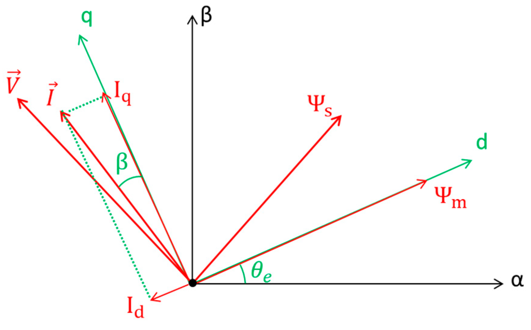
The purpose of applying the MTPA strategy is to minimize copper losses and thus optimize the machine efficiency by calculating the accurate ${\mathrm{I}}_{\mathrm{d}}$ and ${\mathrm{I}}_{\mathrm{q}}$ currents with the optimum angle of the stator current vector. Therefore, the necessity of solving the current angle $\mathsf{\beta }$, given in (1), to provide maximum torque with minimum stator current magnitude is a widely used MTPA method in the literature [25,26].

$$\mathsf{\beta }={\mathrm{s}\mathrm{i}\mathrm{n}}^{-1}\left({\displaystyle \frac{-{\mathsf{\Psi }}_{\mathrm{m}}+\sqrt{{{\mathsf{\Psi }}_{\mathrm{m}}}^2+8{\left({\mathrm{L}}_{\mathrm{q}}-{\mathrm{L}}_{\mathrm{d}}\right)}^2{{\mathrm{I}}_{\mathrm{s}}}^2}}{4\left({\mathrm{L}}_{\mathrm{q}}-{\mathrm{L}}_{\mathrm{d}}\right){\mathrm{I}}_{\mathrm{s}}}}\right)$$

(1)

where ${\mathrm{I}}_{\mathrm{s}}$ represents the stator current magnitude, ${\mathsf{\Psi }}_{\mathrm{m}}$ represents the magnet flux linkage value, and ${\mathrm{L}}_{\mathrm{d}}$ and ${\mathrm{L}}_{\mathrm{q}}$ represent the -dq axes inductance values, respectively. In addition, Figure 1 shows the vector diagram corresponding to the stator current angle calculated in (1).

However, since the conventional equation does not theoretically take the ${\mathrm{L}}_{\mathrm{d}}$, ${\mathrm{L}}_{\mathrm{q}}$, and ${\mathsf{\Psi }}_{\mathrm{m}}$ parameter variations into account, the drive may deviate from the optimal MTPA points in practical applications, unlike the simulation environment [28]. Yet, the real MTPA points can still be accurately obtained using the conventional equation, as long as the ideal machine model is represented in simulation studies. Although the motor parameters are nonlinear in practice, the use of the $\mathsf{\beta }$ angle obtained from the conventional equation given in (1) is still adopted to achieve precise torque control, which is possible as long as accurate parameters are adopted in the conventional equation. In other words, by compensating for parameter variations in the conventional equation, the torque gap can be closed in practical applications [25,27,29]. The torque-controlled IPM drive with the MTPA strategy has been improved by estimating nonlinear parameters of the machine with the parameter estimation algorithm in [29]. Similarly, in [27], the torque gap was closed by developing the MTPA by online estimation of the ${\mathrm{L}}_{\mathrm{d}}$, ${\mathrm{L}}_{\mathrm{q}}$, and ${\mathsf{\Psi }}_{\mathrm{m}}$ parameters. Hence, it is evident in the literature that numerical solutions are still adopted in modern drives to overcome the challenging problems pertinent to optimized current command generation in FOC drives. Although there are other strategies to obtain the optimized current angle, such as the perturb and observe algorithm (P&O), real signal injection, virtual signal injection, and other search methods [30,31,32,33], each has some practical issues. It is known that P&O and search-based strategies may have stability issues in rapid speed variation conditions. Additionally, signal-injection-based optimization strategies, regardless of the use of real or virtual signal injection, increase complexity, implementation difficulty, and total harmonic distortions (THDs) in phase currents, and thereby increase undesired torque ripples in a real-world drive [19]. Moreover, as is well known, there may be humming noise issues in signal-injection-based drives. Thus, obtaining optimized control points through numerical solutions may still be advantageous. This paper adopts numerical solutions to obtain current commands for the test system.

In recent years, innovative methods that also take nonlinear effects into account in order to improve the MTPA control performance in IPM drives have been developed. In [34], a virtual signal-injection-based MTPA method is presented, and the negative effects of cross-coupling, iron loss, and temperature on the control accuracy are reduced by online calculations. In [35], an online MTPA strategy is proposed, where the MTPA strategy is modified by using the proposed Gradient Projection Descent technique. It is shown that the proposed technique is advantageous in terms of computational efficiency and control accuracy when compared to the Levenberg–Marquardt algorithm used for online MTPA calculation. In [36], the problems of lookup table (LuT)-based MTPA strategies, or the need to know the actual machine parameters for accurate MTPA determination, are discussed, and an equivalent base current technique that avoids these problems is proposed. Comparisons conducted in the study also show that the proposed strategy has a lower computational burden than conventional MTPA strategies in real-time tests. In addition, in [37], the nonlinear flux linkage model of IPMs was applied to the MTPA model, and experimental studies showed that more accurate results were obtained compared to a conventional MTPA strategy. In [38], an MTPA strategy was improved that generates an objective function based on the torque/stator current ratio from the machine model with a small DC position offset injection and tracks the MTPA angle rapidly and independently of parameter changes using online curve fitting. As can be seen from these studies, MTPA strategies are improved by considering the nonlinearities of the machine. However, rather than improving the MTPA strategy, this study compares the conventional MTPA strategy with the ${\mathrm{I}}_{\mathrm{d}}=0$ control strategy to verify the correct operation of the components in the IPM drive system.

To handle the challenge to generate IPM drive current commands from a given torque command (due to the high system nonlinearities in practice as well as the requirement to utilize reluctance torque production), there are studies reported in the literature which compare the ${\mathrm{I}}_{\mathrm{d}}=0$ control strategy and current command generation utilizing Equation (1) [24,39,40,41,42]. The researchers in [24,26,39,40] make the comparisons in the simulation environment with particular attention to efficiency, torque, and stator current magnitudes, and it is evident that the drives utilizing Equation (1) achieve higher efficiencies for IPM machines. However, these studies lack practical implementation and therefore do not cover the potential issues that may arise during test system configuration. Refs. [41,42], on the other hand, make their comparisons with practical results and validate their proposed strategies by paying particular attention to improved accuracy. In this paper, however, unlike the above comparative studies, step by step implementation of IPM drive system development in real-world situations is the focus, achieved by paying attention to potential issues in test rigs and discussing accurate calibrations. Since the practical issues that may arise during test system setup are demonstrated using solutions in the paper, the procedures will be quite insightful for researchers willing to set up a drive system as well. Extensive comparative studies using different operating conditions have been carried out with ${\mathrm{I}}_{\mathrm{d}}=0$- and MTPA-controlled drives. In addition, by comparing the ${\mathrm{I}}_{\mathrm{d}}=0$ and MTPA strategies, it was analyzed how the offset value of the initial position angle could affect the MTPA strategy, and it was revealed that this comparison could be used for alignment.

2. Materials and Methods

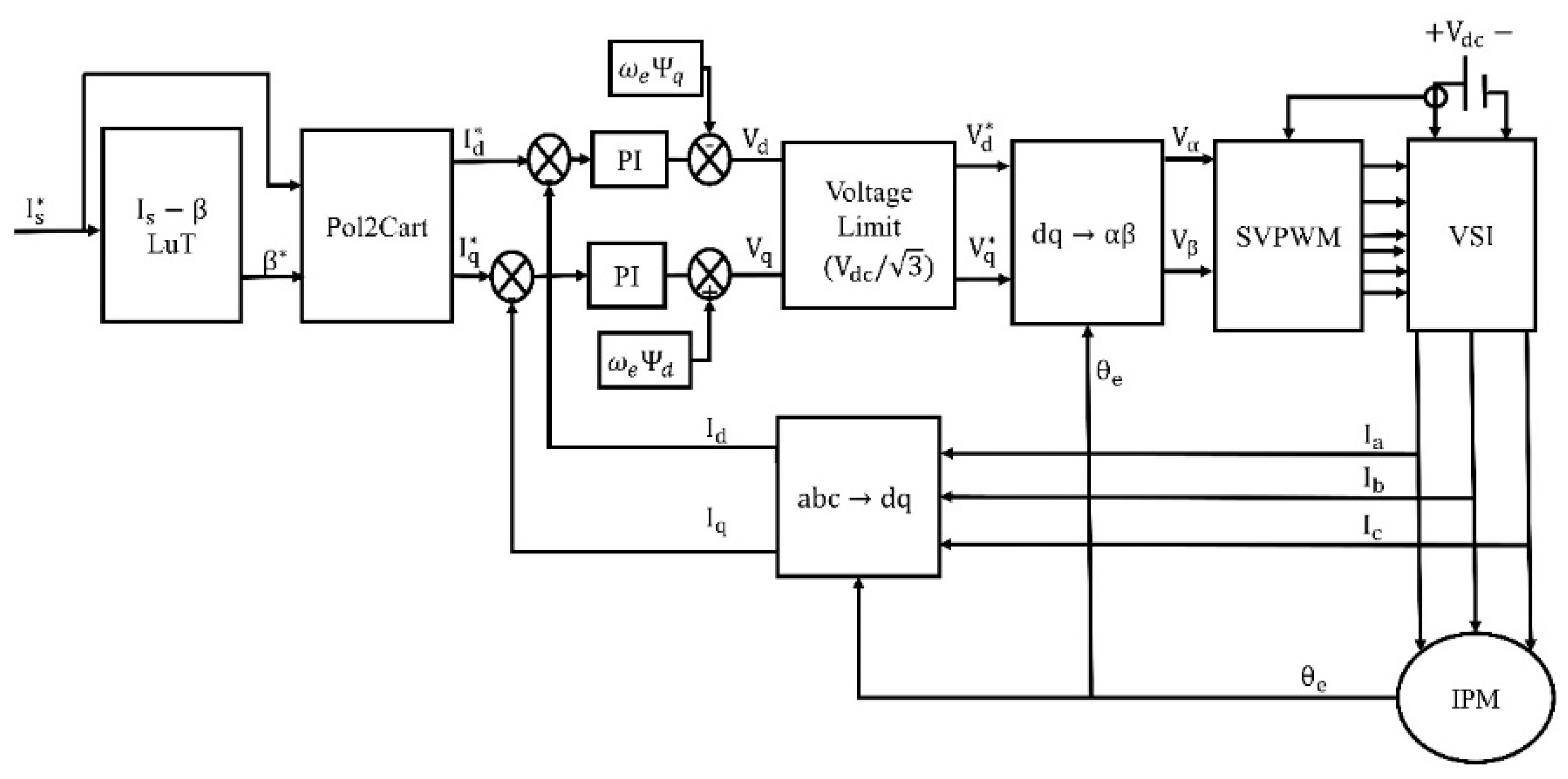
Figure 2 illustrates the block scheme of an IPM drive. As can be seen from Figure 2, in the FOC technique, the -dq axes errors are driven to zero by comparing the reference and the measured -dq axes currents [43]. The -dq axes constitute the rotating rotor reference frame and the -d axis is aligned with the rotor position angle.

Clark and Park transformations are vital for the FOC-based IPM drive implementation. These coordinate transformations are needed to control 3-phase machines, similar to control of DC machines. In order to control 3-phase AC machines in rotationary frame, first the equations in the stationary ABC frames are transformed into the αβ stationary frame using Clark equations, where α is aligned with phase A. Then, with the Park transformation, variables in αβ frame are transformed from a stationary frame into a rotating system defined by the -dq axes (rotor frame), and the control is achieved by separating the variables on the ABC axes into -d and -q axes utilizing peak convention [44]. The error between the command and the measured -dq axes currents is regulated with the help of two PI controllers. Reference -dq axes voltages are produced as the output of PI controllers and transmitted into the pulse width modulation block to generate the necessary gate signals for the voltage source inverter (VSI). As has been widely discussed in the literature, space vector pulse width modulation (SVPWM) is rather superior to other modulation techniques due to having higher battery utilization, less switching loss formation, fewer harmonic distortions, and so on [45,46,47]. Hence, the most common SVPWM strategy is employed throughout the manuscript. Since the αβ stationary frame voltages are needed to obtain the reference voltage vector for SVPWM implementation, inverse Park transformation is adopted before the SVPWM block in Figure 2. In addition, in order to maintain voltage limits (${\mathrm{V}}_{\mathrm{D}\mathrm{C}}/\sqrt{3}$), an over-modulation block is designed and applied in the drive. Further details associated with the SVPWM implementation strategy can be found in [46]. The FOC-based control scheme given in Figure 2 shows the current-controlled IPM drive. Although the input in real-time applications may be speed commands in some cases, this is not the case in electric vehicle traction applications. Also, optimized control strategies can only be obtained when stable current control is achieved with improved torque production for a given stator current magnitude. Hence, the input is not speed commands in this case study.

Mathematical modeling of IPM machines is given by (2)–(4) [48].

$$\left[\begin{array}{c}{\mathrm{V}}_{\mathrm{d}}\\ {\mathrm{V}}_{\mathrm{q}}\end{array}\right]=\mathrm{R}\left[\begin{array}{c}{\mathrm{I}}_{\mathrm{d}}\\ {\mathrm{I}}_{\mathrm{q}}\end{array}\right]+{\displaystyle \frac{\mathrm{d}}{\mathrm{d}\mathrm{t}}}\left[\begin{array}{c}{\mathsf{\Psi }}_{\mathrm{d}}\\ {\mathsf{\Psi }}_{\mathrm{q}}\end{array}\right]+\mathsf{\omega }\left[\begin{array}{c}-{\mathsf{\Psi }}_{\mathrm{q}}\\ {\mathsf{\Psi }}_{\mathrm{d}}\end{array}\right]$$

(2)

$$\left[\begin{array}{c}{\mathsf{\Psi }}_{\mathrm{d}}\\ {\mathsf{\Psi }}_{\mathrm{q}}\end{array}\right]=\left[\begin{array}{cc}{\mathrm{L}}_{\mathrm{d}}& 0\\ 0& {\mathrm{L}}_{\mathrm{q}}\end{array}\right]\left[\begin{array}{c}{\mathrm{I}}_{\mathrm{d}}\\ {\mathrm{I}}_{\mathrm{q}}\end{array}\right]+\left[\begin{array}{c}{\mathsf{\Psi }}_{\mathrm{m}}\\ 0\end{array}\right]$$

(3)

$${\mathrm{T}}_{\mathrm{e}}={\displaystyle \frac{3\mathrm{p}}{2}}\left({\mathsf{\Psi }}_{\mathrm{m}}{\mathrm{I}}_{\mathrm{q}}-{\mathrm{I}}_{\mathrm{d}}{\mathrm{I}}_{\mathrm{q}}\left({\mathrm{L}}_{\mathrm{q}}-{\mathrm{L}}_{\mathrm{d}}\right)\right)$$

(4)

where ${\mathrm{V}}_{\mathrm{d}}$ and ${\mathrm{V}}_{\mathrm{q}}$ are the voltage magnitudes (Volt) and ${\mathrm{I}}_{\mathrm{d}}$ and ${\mathrm{I}}_{\mathrm{q}}$ are the current magnitudes (A) in the -dq frame, $\mathrm{\omega }$ is the electrical speed in rad/s, p is the pole-pair number, ${\mathrm{L}}_{\mathrm{d}}$ and ${\mathrm{L}}_{\mathrm{q}}$ are the inductance values (H) of the -d and -q axes, respectively, ${\mathsf{\Psi }}_{\mathrm{m}}$ is the permanent magnet flux linkage (Wb), and R is the stator resistance (ohm). ${\mathrm{T}}_{\mathrm{e}}$ is the electromagnetic torque in Nm. ${\mathsf{\Psi }}_{\mathrm{d}}$ and ${\mathsf{\Psi }}_{\mathrm{q}}$ are flux magnitudes (Weber) in the -dq frame. Since ${\mathrm{L}}_{\mathrm{d}}$ and ${\mathrm{L}}_{\mathrm{q}}$ are equal in SPMs, the inductance values can be represented as ${\mathrm{L}}_{\mathrm{s}}$.

The equations for the MTPA strategy, where maximum torque production can be achieved with minimum stator current magnitude, are given in (1), (5), and (6) [49].

$$\left[\begin{array}{c}{\mathrm{I}}_{\mathrm{d}}\\ {\mathrm{I}}_{\mathrm{q}}\end{array}\right]={\mathrm{I}}_{\mathrm{s}}\times \left[\begin{array}{c}-\sin \mathrm{\beta }\\ \cos \mathrm{\beta }\end{array}\right]$$

(5)

$$\left|{\mathrm{I}}_{\mathrm{s}}\right|=\sqrt{{{\mathrm{I}}_{\mathrm{d}}}^2+{{\mathrm{I}}_{\mathrm{q}}}^2}$$

(6)

Once the current angle is obtained, the -dq axes currents can easily be obtained using (5) and (6). As can be seen from Equations (7) and (8), IPMs are capable of generating reluctance torque due to the differences in the ${\mathrm{L}}_{\mathrm{d}}$ and ${\mathrm{L}}_{\mathrm{q}}$ values. If the IPMs are driven with the ${\mathrm{I}}_{\mathrm{d}}=0$ control technique, the machine can only generate torque equal to the magnet torque in (7). However, by using the MTPA strategy, it is also possible to generate the reluctance torque in (8). This will increase the torque the IPM can produce at the same current value, thus increasing the drive’s efficiency.

$${\mathrm{T}}_{\mathrm{e}\_\mathrm{m}\mathrm{a}\mathrm{g}\mathrm{n}\mathrm{e}\mathrm{t}}={\displaystyle \frac{3\mathrm{p}}{2}}{\mathsf{\Psi }}_{\mathrm{m}}{\mathrm{I}}_{\mathrm{q}}$$

(7)

$${\mathrm{T}}_{\mathrm{e}\_\mathrm{r}\mathrm{e}\mathrm{l}\mathrm{u}\mathrm{c}\mathrm{t}\mathrm{a}\mathrm{n}\mathrm{c}\mathrm{e}}={\displaystyle \frac{3\mathrm{p}}{2}}\left({\mathrm{I}}_{\mathrm{d}}{\mathrm{I}}_{\mathrm{q}}\left({\mathrm{L}}_{\mathrm{d}}-{\mathrm{L}}_{\mathrm{q}}\right)\right)$$

(8)

3. Simulation Results

As can be seen in Figure 2, the commands of the system are the stator current magnitude and the current angle $\mathsf{\beta }$. If the drive is operated by setting the $\mathsf{\beta }$ angle to 0, the IPM is controlled with the ${\mathrm{I}}_{\mathrm{d}}=0$ control strategy. However, if the system is operated with the optimal $\mathsf{\beta }$ value corresponding to a given stator current magnitude, then the IPM uses the MTPA strategy. The specifications of the prototype machine under study are listed in

Table 1. Machine specifications.

Type	IPM
Number of Phases	3
Number of Pole Pairs	4
Continuous Torque	15.7 Nm-@51.6 Arms
Peak Torque	50 Nm-@165 Arms
Nominal Speed	2500 rpm-@120 V DC
Maximum Speed	10,000 rpm-@120 V DC
Continuous Power	4.1 kW-@120 V DC
-dq Axes Inductances	${\mathrm{L}}_{\mathrm{d}}=0.282$ mH, ${\mathrm{L}}_{\mathrm{q}}=0.828$ mH
Flux Linkage	${\mathsf{\Psi }}_{\mathrm{m}}=0.0182$ Wb
Stator Resistance	${\mathrm{R}}_{\mathrm{s}}=0.0463$ Ω
Inertia	J = 0.0071572 kg $\times$ m2
Input Voltage Range	120 V

, and these have been employed in the simulated machine model as well. Details regarding PI tuning are given in [44]. The inverter switching frequency is set to 8 kHz in the simulated drive.

The $\mathsf{\beta }$ angle corresponding to the given stator current magnitude for the prototype IPM machine has been obtained by the numerical solutions of (1), and the details regarding numerical iterative methods can be found in [26]. The strategy can be implemented using either an online or offline approach. Since online iterative solutions greatly increase the computational burden [26], the ${\mathrm{I}}_{\mathrm{s}}$-$\mathsf{\beta }$ LuT has been formed as shown in Figure 3, and the LuT has been used in the implementation of the MTPA strategy. It is worth noting that the study was conducted using MTPA equations derived without considering machine nonlinearities and magnetic saturation. This is because the aim of this study is to overcome potential problems in the experimental setup by comparing the MTPA and ${\mathrm{I}}_{\mathrm{d}}=0$ control techniques.

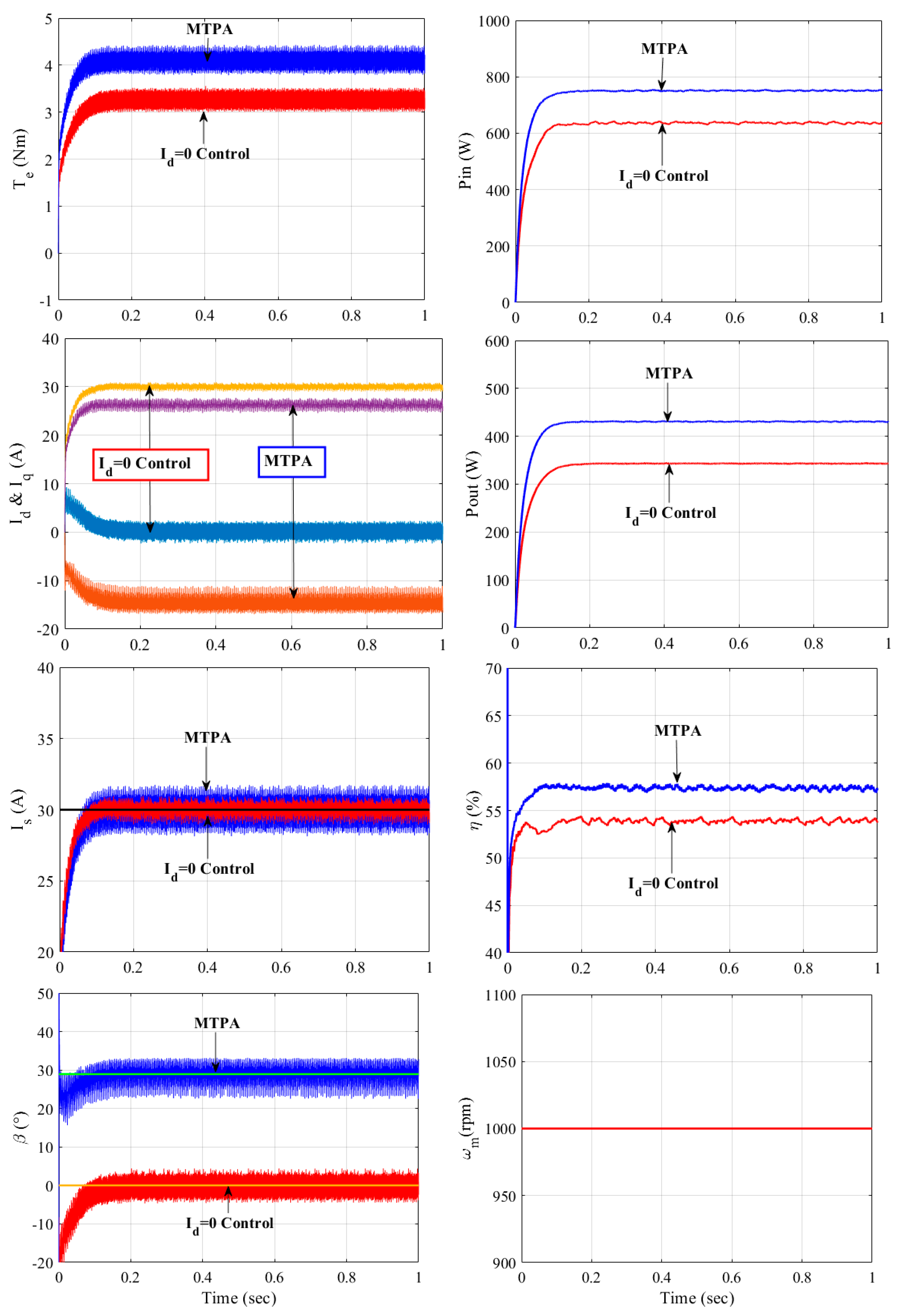
Figure 4 shows comparative results of the FOC-based IPM drive using both the ${\mathrm{I}}_{\mathrm{d}}=0$ and MTPA control strategies. The torque magnitude produced by the machine at 10, 20, and 30 A stator current commands, -dq axes currents, and mechanical speed are presented in Figure 4. The optimal β angles corresponding to 10, 20, and 30 A stator current magnitudes have been previously obtained as 14.77°, 23.89°, and 28.92°, respectively, and they have already been stored as lookup tables in the drive. For fair comparisons in Figure 4, the simulated drives have the same parameters and simulation elements except for the current angle commands. Also, the simulation results have been obtained at the same speed profiles. It is evident from the results that the drive with the MTPA strategy achieves higher torque production than the drive with the ${\mathrm{I}}_{\mathrm{d}}=0$ control strategy when the machine operates at standstill and in transition and constant speed states. Based on the results, it is clear that to produce the same torque, the ${\mathrm{I}}_{\mathrm{d}}=0$-controlled drive will need more stator current, and therefore the efficiency will be lower.

Figure 5 compares the actual torque values, input and output powers, and motor efficiencies of both drives at the same stator current magnitude and the same operating speed conditions, where the machines operate at constant 1000 rpm mechanical speed. Figure 5 validates that the MTPA strategy achieves ~1 Nm higher torque production, and this leads to ~4% higher motor efficiency at the same stator current magnitude operation. The equations employed to compare the input and output powers and the efficiencies in Figure 5 are given by (9)–(11) [26]. ${\mathsf{\omega }}_{\mathrm{m}}$ in (10) is the mechanical speed in rad/s.

$${\mathrm{P}}_{\mathrm{i}\mathrm{n}}={\displaystyle \frac{3}{2}}\times ({\mathrm{V}}_{\mathrm{d}}\times {\mathrm{I}}_{\mathrm{d}}+{\mathrm{V}}_{\mathrm{q}}\times {\mathrm{I}}_{\mathrm{q}})$$

(9)

$${\mathrm{P}}_{\mathrm{o}\mathrm{u}\mathrm{t}}={\mathsf{\omega }}_{\mathrm{m}}\times {\mathrm{T}}_{\mathrm{e}}$$

(10)

$$\mathsf{\eta }\mathrm{\%}={\displaystyle \frac{{\mathrm{P}}_{\mathrm{o}\mathrm{u}\mathrm{t}}}{{\mathrm{P}}_{\mathrm{i}\mathrm{n}}}}\times 100$$

(11)

4. Experimental Results

Figure 6 shows the test setup of the prototype IPM drive. The DC power supply (actually a battery simulator), which is connected to the grid, has a programmable DC output voltage level of 0–1500 V with an output power capacity of up to 15 kW. It is connected to a commercial inverter with a DC bus maximum voltage rating of 1100 V and a maximum AC output voltage of 530 V. The characteristics of the prototype IPM machine are given in Table 1. The DC power supply in the system has been operated at the voltage level of 120 V due to machine constraints.

The dSpace-RTI 1202 MLBX was employed as the controller in the machine drive system. The generated codes can be loaded into the device through the ControlDesk 6.1 software developed by dSpace. The signal outputs received from the dSpace controller are at a 5 V level. However, the inverter requires the signals at a 24 V level. An optocoupler circuit was designed to provide isolation between the dSpace and the inverter and to feed the inverter by pulling the 5 V level signal to 24 V level. In addition, the auxiliary power supply is supported by a UPS connection to prevent the inverter from experiencing a momentary outage due to the risk of power failure.

A dynamometer is employed to keep the machine operation speed at the desired level, and the load torque of the passive dyno is controlled by its input current. In addition, a commercial torque transducer is employed for accurate torque measurement. The nominal torque level of the transducer is 20 Nm. As can be deduced from Table 1, the transducer is suitable for the test system since the continuous torque capacity of the machine is 15.7 Nm.

4.1. Implementation of FOC-Based Test System Using dSpace 1202

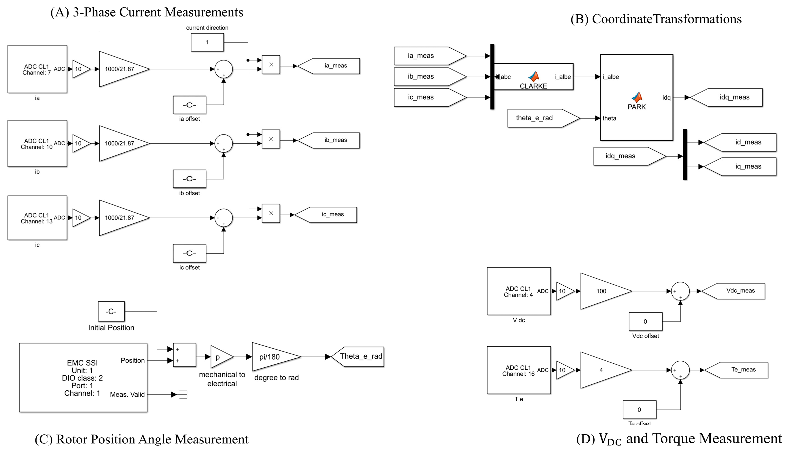
In Figure 7, the dSpace blocks facilitate critical aspects essential for the FOC technique, containing the measurements of phase currents, DC bus voltage, rotor position angle, and the electromagnetic torque via a torque transducer. Alignment of the rotor position angle with respect to phase A is crucial to achieve stable torque control; obtaining the initial rotor position angle will be discussed later in detail. 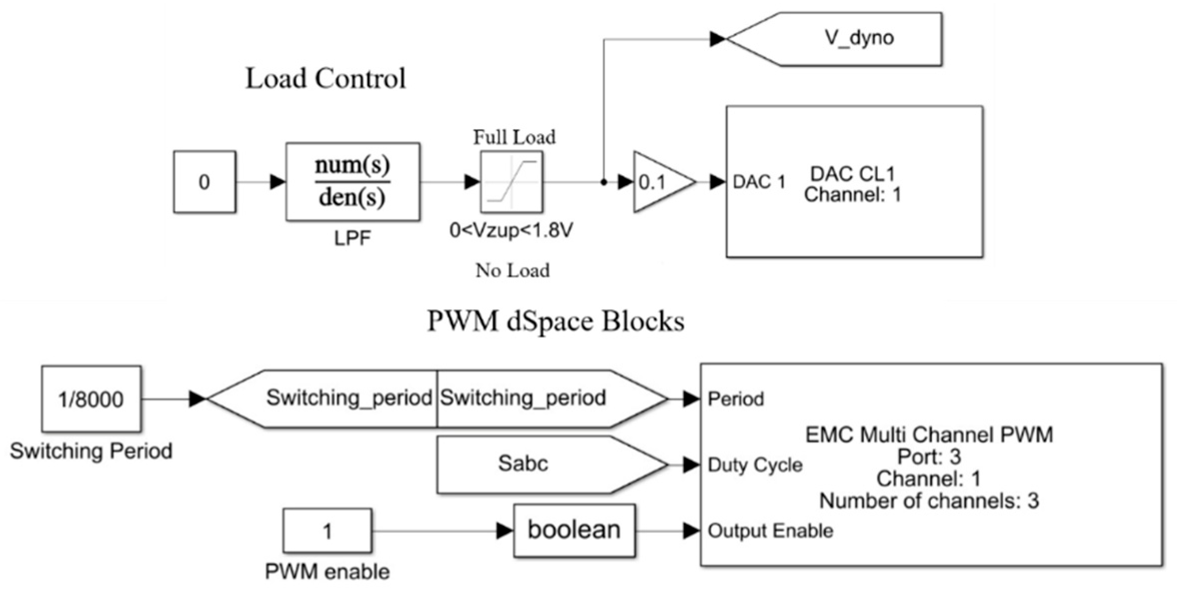Figure 8 illustrates the dSpace elements for schematic representation of the load control and delivering gate signals into the IGBT drivers at the desired switching frequency. It should be noted that S_abc shown in Figure 7 is obtained from the SVPWM strategy and represents duty ratios of semiconductor switches. It should also be noted that the dSpace has a built-in gain of 1/10×and 10× in DAC and ADC conversions, respectively. Also, the dyno (braking load) is controlled by a current source. Hence, its controller has been configured as a voltage-controlled current source, and the dyno controller in the case study generates 2.84 A (corresponds to ~34 Nm full load) once 1.8 V is applied to its input via dSpace 1202 analog output. In short, the dyno is controlled by the dSpace, and its dedicated DAC pin varies between 0 V and 1.8 V, referring to no load and full load, respectively.

4.2. $I_d=0$-Controlled Drive

The results obtained from the ${\mathrm{I}}_{\mathrm{d}}=0$-controlled drive shown in Figure 9 validate that the stable FOC-based control has been successfully achieved owing to necessary ADC and DAC conversions shown in Figure 7 and Figure 8. Figure 9 shows the filtered form of measured electromagnetic torque obtained from the torque transducer for clearer illustration. In addition, instantaneous phase currents received from the current transducers are monitored. The measured and calibrated phase currents are transformed into -dq axes currents with Clark and Park transformations, as shown in Figure 7, and employed in the controller to achieve control in the rotating reference frame. The stator current magnitude, ${\mathrm{I}}_{\mathrm{s}}$, is obtained from measured -dq axes currents by (6) and monitored via Controldesk as shown in Figure 9.

Figure 9 and Figure 10 belong to the same test, and Figure 10 validates the accurate implementation of the SVPWM strategy. Sector transitions based on the rotor position and the duty ratios are illustrated in Figure 10. After obtaining the -dq axes voltages at the output of the PI controllers with necessary coupling compensations in (2), they are transformed into the αβ stationary frame with the Clark equations. It should be noted that the coupling compensations are only needed when speed varies rapidly since the compensation improves the transient response and has theoretically no influence at steady states. Duty ratios are obtained by performing the modulation process using the voltage vector magnitude, its load angle, and the rotor position angle. The sector where the voltage vector lies is determined, and the obtained gate signals are delivered to the IGBT drivers at the desired switching frequency through the dedicated pins of dSpace, as shown in Figure 8. In this study, the switching frequency for SVPWM is set to 8 kHz, as in the simulation studies. It is important to note that the switching frequency is determined by the trade-off between reduced THD (improved current quality) and the increased power-electronics-based system losses in practical drives. Clearly, the switching frequency cannot be lower than the operating electrical frequency, as there will be issues with the control, such as the stability problem and sampling errors. The maximum electrical frequency in the case study is 667 Hz, which corresponds to 10 krpm mechanical speed. Typically, the switching frequency is determined as 5 to 10 times of the maximum electrical frequency [50]. It has also been noted that when the operations are at relatively lower switching frequencies, such as 1 kHz, the THD increases considerably, and audible noise issues such as whistling arise. On the other hand, it has also been noted that increasing the switching frequency to a considerably high level reduces current THDs at only marginal levels, and the improvement is smaller, as the losses theoretically become significant in that case. Hence, a typical sampling period is reasonable, and the PWM has been adopted with a sampling time of 125 µs in the case study in both the simulation and experiment.

Utilizing (9)–(11), instantaneous values of the machine’s input power, output power, and efficiency have been recorded from the same ${\mathrm{I}}_{\mathrm{d}}=0$-controlled test, and the results are plotted in Figure 11. Similar to the measured torque illustration, low-pass filters with low time constants have been adopted for clear illustration of the input power, output power, and efficiency of the IPM machine. It should be noted that the tested machine is deliberately operated at low speed and torque profiles to make sure that the test system achieves stable operation. Accordingly and expectedly, the efficiency is relatively lower than the rated operating conditions.

4.3. MTPA-Controlled Drive

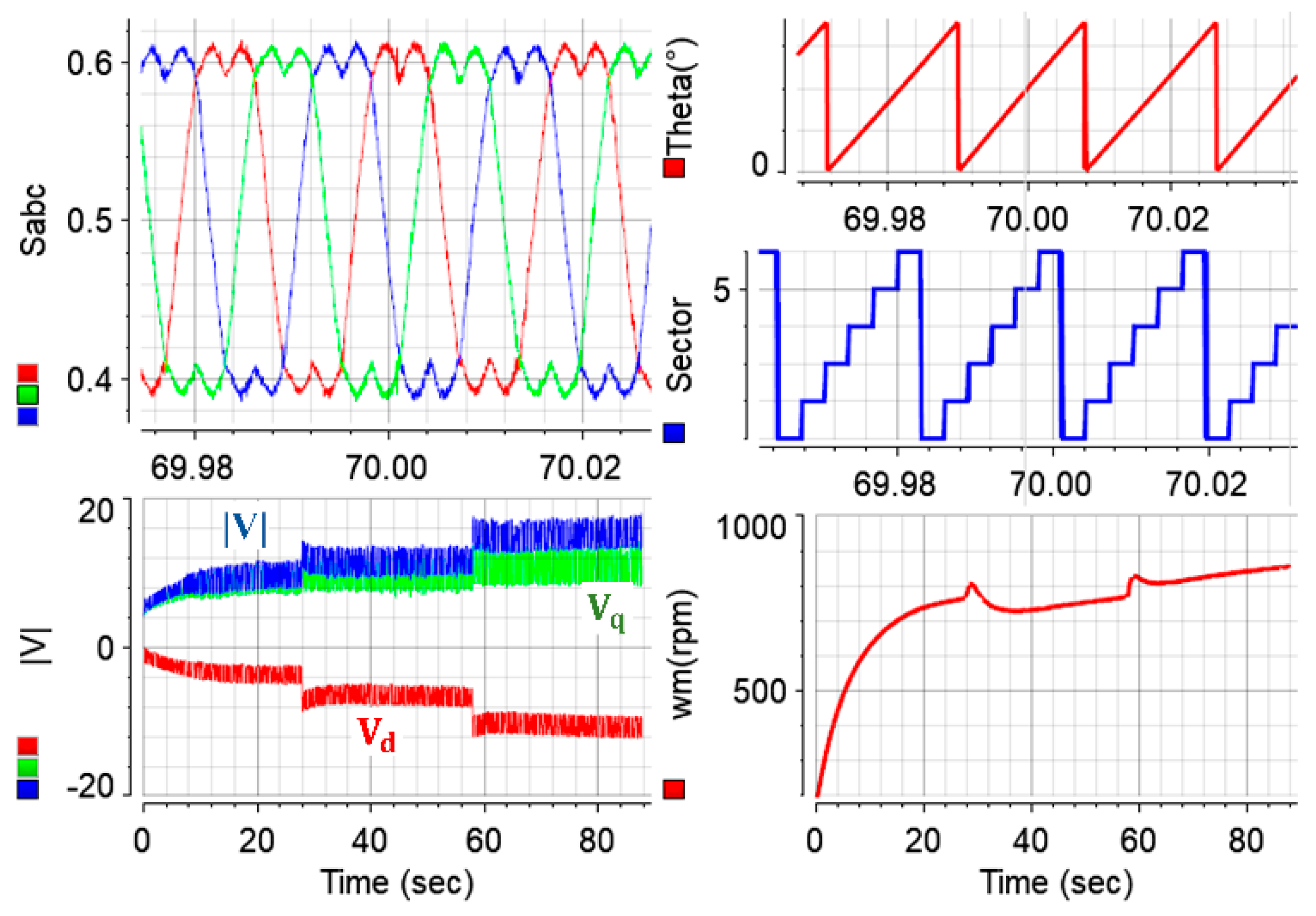
As discussed, the MTPA strategy for IPMs is important to utilize the reluctance torque production capability. As simulation results validate the significance of MTPA control to achieve higher torque production as well as higher efficiency operation, the strategy has also been experimentally validated with extensive tests, and the results are presented comprehensively in Figure 12. The measured electromagnetic torque produced by the IPM drive with the MTPA strategy, the waveforms of measured three-phase currents, measured and command -dq axes currents, the stator current command and its measured value, duty ratios generated by the SVPWM strategy, the sector where the voltage vector lies and the rotor position angle, the command -dq axes voltages and voltage magnitude, current angle β, input and output powers of the machine and its efficiency, and the operation speed are all illustrated in Figure 12. It is noteworthy that illustrating multiple state variables at one glance during experiments is quite insightful to study and understand the operation principle of the test drive, as it facilitates simple determination of the reason behind any potential issues. As evident in Figure 12, the drive achieves stable control of both -d and -q axes currents as their errors are driven to zero. As can be seen, the -d axis current magnitude is increased in the negative direction as torque increases (viz. the MTPA). One can deduce from Figure 12 that the operation speed freely varies based on the difference between the electromagnetic torque and the load torque. This is as expected since the drive operates under torque-control mode. Once the electromagnetic torque is higher than the load torque, the machine speed increases, and vice versa. As discussed earlier, the machine is deliberately operated below base speed, and one can deduce from Figure 12 that the efficiency increases when the machine approaches the base speed, and vice versa.

4.4. Comparisons of $I_d=0$- and MTPA-Controlled Drives

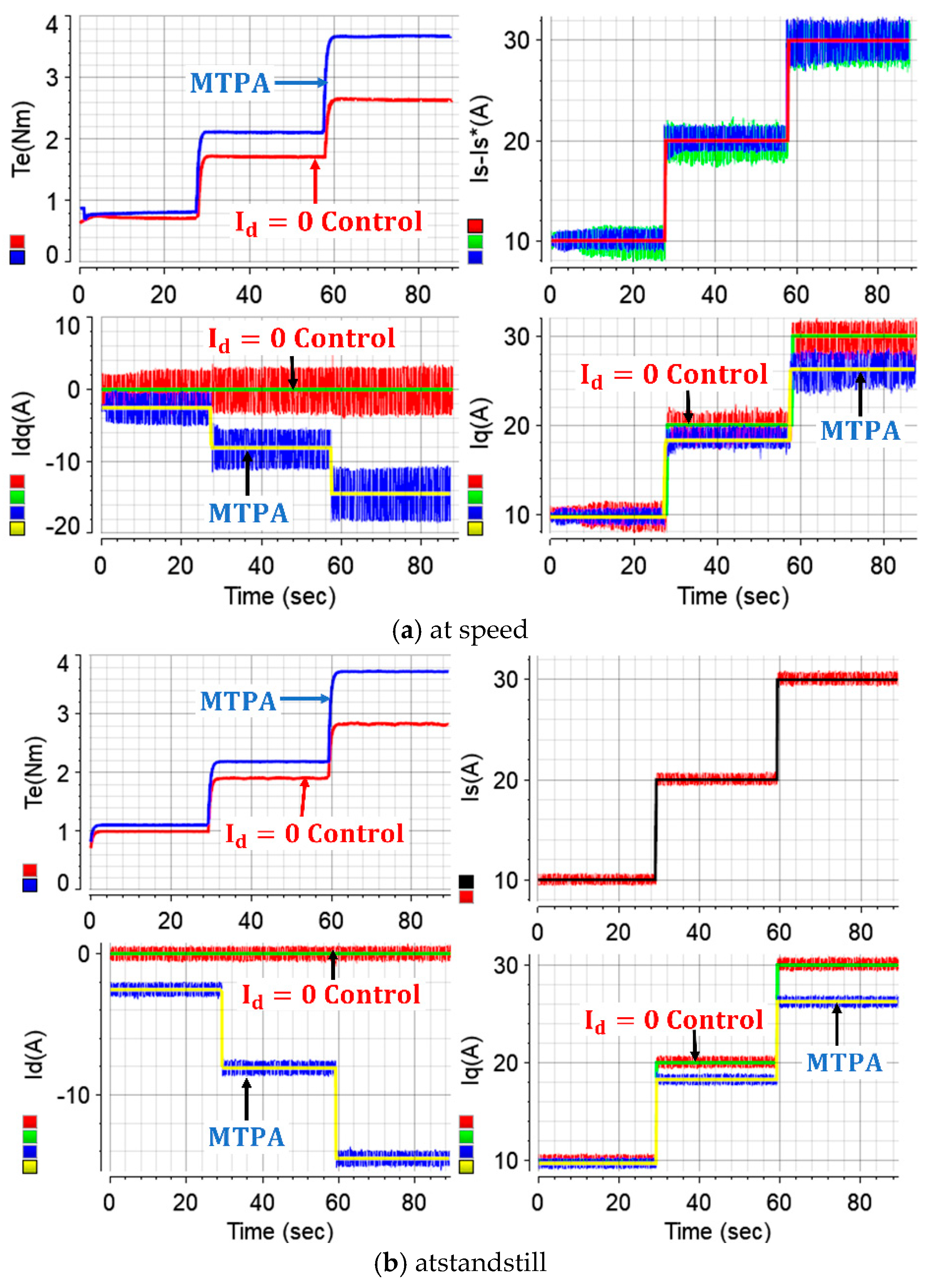
The ${\mathrm{I}}_{\mathrm{d}}=0$- and MTPA-controlled drives are compared in Figure 13. Although the two drives are operated separately, the current and torque responses in both drives are superimposed in Figure 13 for ease of comparison. It is noteworthy that the drives do not operate at the same speed profile. As explained, the speed freely varies, but it is kept within one-third of the base speed with the brake. This is because the drives are deliberately operated in the torque (current)-control mode. Due to the different speed profiles, the input/output powers and the efficiencies of the machines in both drives are not compared in Figure 13. However, it is important to note that the torque production in the constant torque region is theoretically independent from the operating speed, as evident in (4). Hence, Figure 13 fairly compares the torque production capabilities of both strategies at the same stator current magnitude. The figure also illustrates the -dq axes commands and measured currents of both drives. Although both drives are operated at the same 30 A stator current magnitude, as seen in Figure 13a, ~2.6 and ~3.7 Nm torque have been produced by the ${\mathrm{I}}_{\mathrm{d}}=0$- and MTPA-controlled drives, respectively. It is evident that utilization of the reluctance torque production capability of IPM machines by approaching the optimum current angle β trajectory increases the total electromagnetic torque production. The ~1.1 Nm higher torque production at 30 A in the case study matches well with the simulation results shown in Figure 5. The same phenomenon as in Figure 13a is also valid for Figure 13b, where the operation is performed at standstill. One can deduce from Figure 13 that the measured -dq axes currents have relatively high ripples. Indeed, this is as expected since the machine inductance is relatively lower than its typical counterparts.

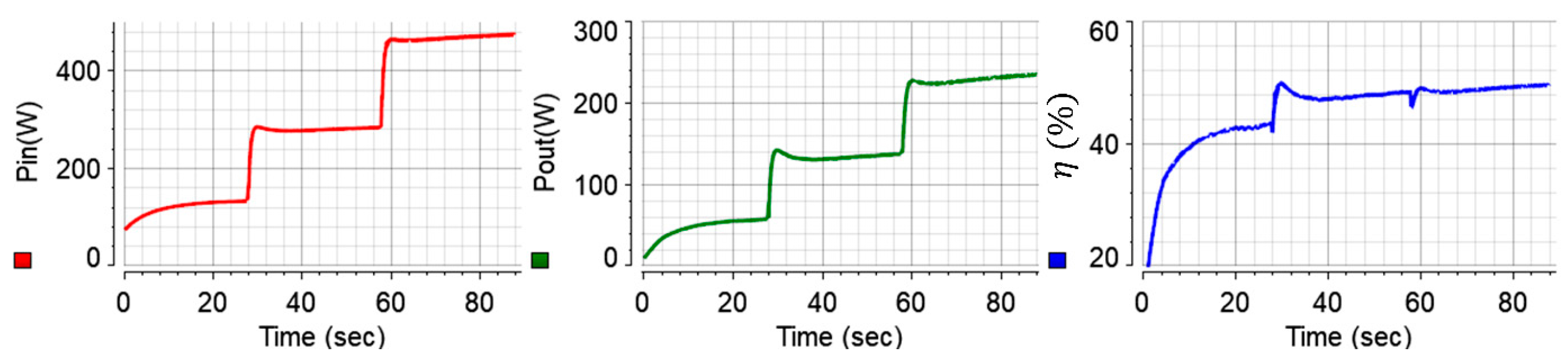
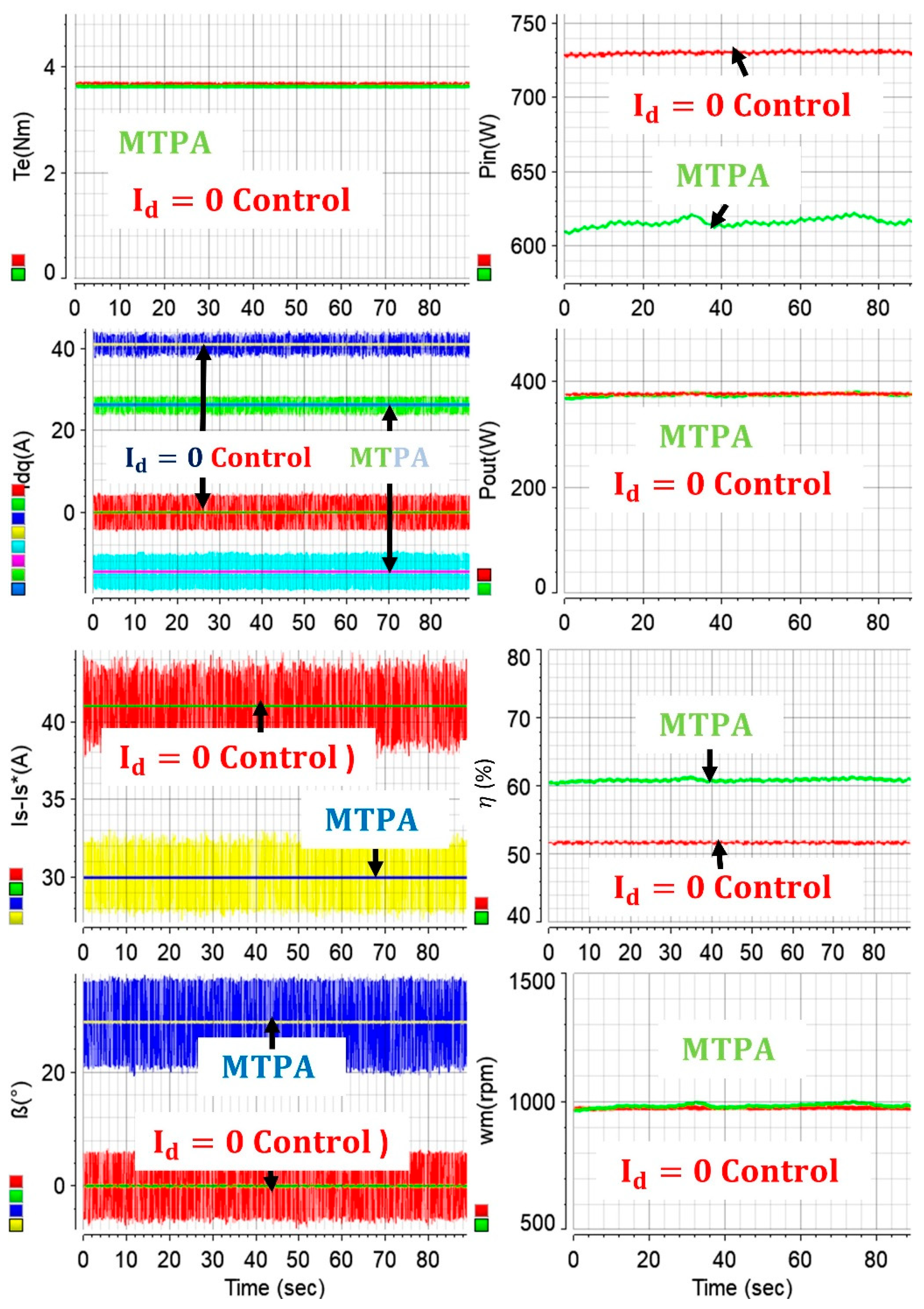
Comparative results have been further carried out. Unlike standstill or varying speed operations in Figure 13, both drives were operated around 1000 rpm, and the input/output powers, motor efficiencies, stator current magnitudes, -dq axes currents, $\mathsf{\beta }$ angles, and torque values of both approaches are presented in Figure 14. The drives have been operated to produce same output torque, and hence, based on (8), the output powers of the drives are similar. Therefore, the input powers of the drives illustrate the required powers to generate similar outputs. It is evident at this particular operating point that utilization of bonus reluctance torque in IPM drives greatly improves the system efficiency since the required input power is ~110 W less. This power corresponds to ~9 percent energy efficiency at the given operating point, at which the machines achieve same output. This is due to the fact that the utilization of reluctance torque enables achievement of the same total torque with lower stator current magnitude, which is reduced from 41 A to 30 A in the case study, as shown in Figure 14.

4.5. Discussion of Potential Experimental Issues

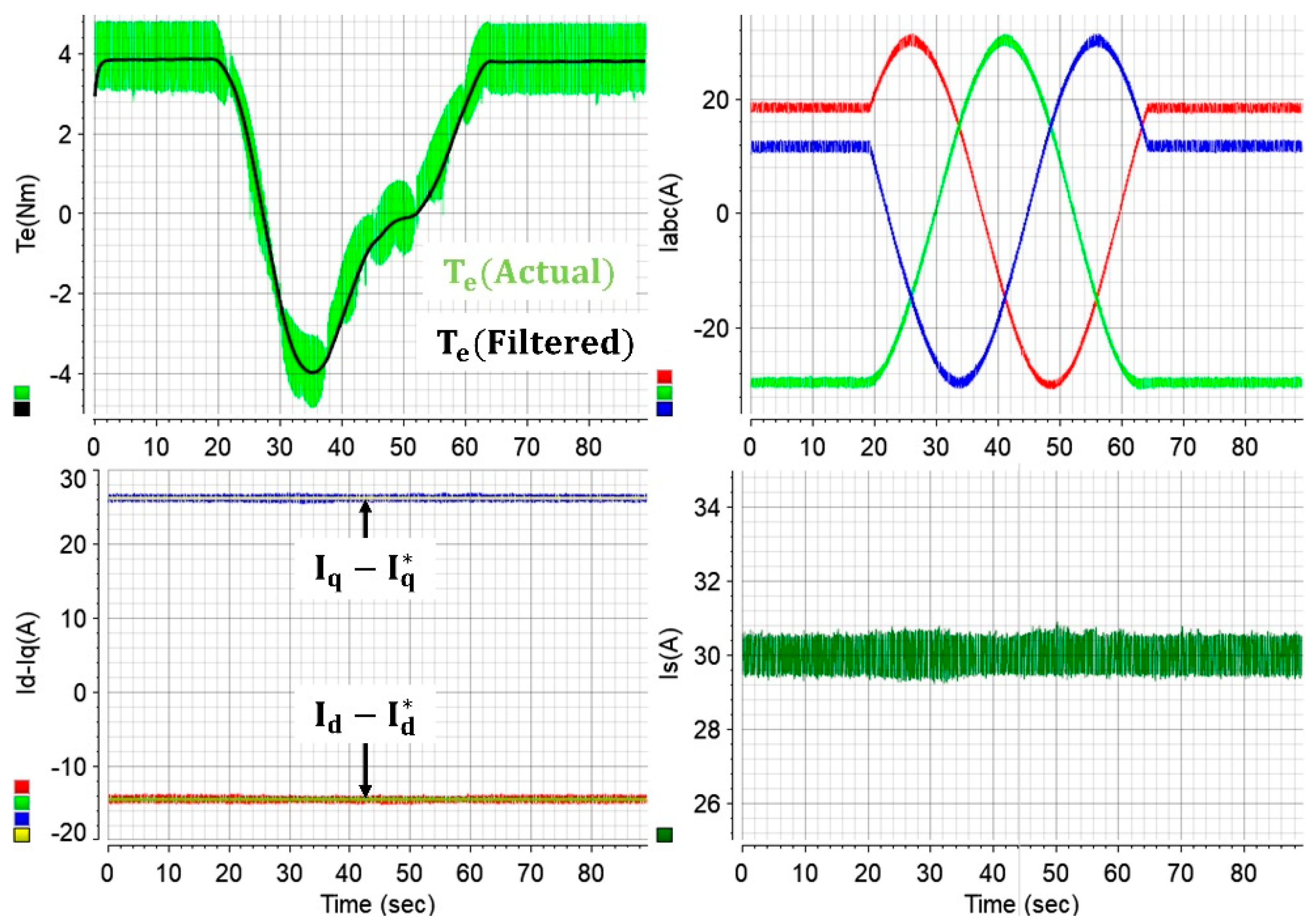
It should be noted that the simulation results and the experimental results do not perfectly match due to the highly nonlinear system parameters and different operating conditions in real-world drives. Temperature variations, PM flux linkage variations, load (and thereby current-magnitude-based motor inductance saturations), manufacturing tolerances, material property variations, stator resistance variations, and the inevitable use of nonlinear power semiconductor devices in power converters are among the leading reasons for nonlinearities in real-world drive systems, and these have significant influences on the overall system performance for a wide range of operations. Once any nonlinearity is represented in a simulation environment, the results better represent real-world drives.

It is crucial in experimental test systems that the rotor position angle is aligned accurately to achieve high efficiency operation. This is indeed challenging in real-world drives. As is known, the FOC strategy is realized in the rotor reference frame, where the -d axis rotates with electrical position angle. Once the initial position angle becomes inaccurate, despite the accurate rotational speed, the -d axis will rotate synchronously (to achieve stable control); however, there will be a gap between the actual and the measured -d axes in experiments. In other words, the measured -dq axes currents will not be accurate, and the deviation will depend on the initial position angle error. For example, once the ${\mathrm{I}}_{\mathrm{d}}=0$ control strategy is adopted with the above issue, the -d axis current error will be monitored as if it is accurately driven to zero, similar to the situation depicted in Figure 15. Stable control is still achieved, but there will be a nonzero -d axis current in the drive system that cannot be monitored. The issue is significant since it will render the efficiency-optimized control impossible. Thus, the untraceable issue is studied in Figure 15. The initial electrical position angle has been deliberately rotated 360°. Starting from ~19 s in Figure 15, the initial angle has been increased with a slope of 8, and hence 360° rotation has been completed in 45 s. Despite the measured -dq axes currents between ~19 and ~64 s being incorrect, the -dq axes currents seem to remain the same, and the drive seems to operate accurately since the current errors are still driven to zero (stable control is still achieved). For example, if the drive is operated with the initial position angle given in second 22, stable control will still be achieved, current errors will still be regulated, and a constant (but smaller) electromagnetic torque will still be produced. However, as evident in Figure 15, maximum electromagnetic torque production cannot be achieved with the inaccurate position alignment. This will lead to deteriorated drive performance and reduced efficiency. The challenge can also be studied from the following perspective. Based on (4), theoretically, the electromagnetic torque cannot be produced when the actual -q axis current is zero. The actual -q axis current will become zero twice during 360° angle rotation, as shown in Figure 15. Hence, the zero actual torque in Figure 15 implies that the actual -q axis current is zero. However, one can deduce from the figure that the alleged -q axis current (measured current) seems to be constant at ~26 A. This validates the misaligned position angle. Also, the peak and reverse peak torque productions can only be achieved with accurate alignment and 180° misalignment, respectively. This can be deduced from Figure 15, where the drive is operated at standstill. It is evident in Figure 15 that a ~40° misaligned rotor position leads to half output torque production. This implies that ~10° misalignment will lead to ~12.5% reduced output power at the same speed. Therefore, accurate alignment is crucial for high efficiency.

It is also noteworthy that to achieve optimized rotor alignment, accurate connection of the phase sequence requires a careful approach. The rotor position angle is aligned with respect to one of the phases, which may be defined as phase A, and then the other two-phase connections do not matter much, as it results in operation in the reverse direction. For example, if ABC sequence achieves clockwise rotation, ACB sequence will operate in counterclockwise rotation. Similarly, if BAC rotates clockwise, BCA rotates counterclockwise. However, it is important to consider that while the rotor position angle needs to be aligned with respect to phase A in the former case, it needs to be aligned with respect to phase B in the latter.

5. Conclusions

Due to their attractive features such as high efficiencies, high torque/power densities, good performance at wide speed range, and so on, widely used IPM drives need to be controlled in such a way that maximization of torque production for efficiency optimization is achieved by utilizing both the magnet-based and reluctance torque production capabilities of these machines, viz. MTPA. In IPM drives, the importance of reluctance torque utilization on the overall system efficiency has been validated by both simulation and experimental results with extensive tests at standstill and at speed, comparing both transient and steady-state responses by using a 4.1 kW prototype IPM machine designed and manufactured for research and development of advanced control strategies for traction applications. It has been shown that utilization of only magnet-based torque production in IPM drives with ${\mathrm{I}}_{\mathrm{d}}=0$ control (due to attractive control simplicity) considerably reduces the torque production capability of the machine. As can be seen from the comprehensive simulation and experimental results, the implementation of the MTPA strategy increased the machine’s generated torque by 42.3%. This allows for the utilization of reluctance torque. This benchmark study can also be used to analyze misaligned position sensor errors to address potential problems in the test system. As can be seen in Figure 15, a position sensor misaligned by ~40° can reduce the torque generation capacity by 50%. This leads to practical issues such as performance deteriorations, greatly reduced drive efficiency, prevention of a compact design approach of system components, early field weakening and thereby narrow speed range operation, prevention of maximum torque production capability that degrades the acceleration performance, and so on. Therefore, an adopted MTPA system configuration has been discussed step by step in detail by paying attention to potential practical issues in real-time experiments. Solutions to these issues, such as misaligned rotor position angle or whistling problems due to inconvenient power conversion strategies, have been discussed in greater detail. In conclusion, this paper paves the way for achieving high performance and efficiency-optimized control of highly nonlinear real-world IPM drives.