1. Introduction
In a decentralized and interconnected power grid, maintaining the balance between generation and consumption within each control region is vital. To ensure that scheduled power exchanges and system frequency remain close to their target values, a precisely designed regulatory strategy, commonly referred to as load frequency control (LFC), is essential. With the growing integration of renewable energy sources and distributed energy resources, maintaining system stability has become significantly more challenging, primarily due to the inherently stochastic and time-varying nature of such sources and their impact on grid dynamics [
1]. As modern power networks expand in scale and complexity, they become increasingly vulnerable to the propagation of oscillations across large regions, increasing the threat of large-scale blackouts. To mitigate these risks, advanced control methodologies have been embedded within LFC architectures to enhance grid resilience and maintain overall system stability.
Traditional LFC strategies commonly employ integral controllers [
2]. A key shortcoming of these controllers is that their dynamic behavior is restricted by the selection and tuning of the integral gain [
3]. Extensive research has focused on enhancing system stability by extending conventional proportional integral (PI) frameworks. However, these efforts often face challenges related to the design and parameter tuning of proportional integral derivative (PID) controllers in the context of load frequency control [
4,
5,
6]. The principal objective of LFC is to eliminate steady-state frequency deviations, accurately follow load variations, and simultaneously ensure that frequency and tie-line power deviations remain within acceptable limits in terms of overshoot and settling time [
7,
8]. Considering the crucial role of LFC, considerable scholarly attention has been directed toward advanced methodologies, such as optimal control [
9,
10], variable structure control [
11], and adaptive control techniques [
12] to improve dynamic performance and robustness. Recently, a wide range of optimization-based approaches have been introduced to enhance the performance of different controllers [
13]. However, in all these approaches, ensuring system stability while meeting user-defined objectives and constraints proves to be computationally expensive [
14]. Moreover, these approaches may require high-fidelity forecasting models or extensive real-time measurements, which may not always be feasible in practical deployments [
15,
16].
While these approaches hold promise for enhancing load frequency control, they are difficult to apply in practice due to unmeasured inputs, system uncertainties, and actuator malfunctions. Such disruptions can significantly affect the performance of the control system. Moreover, when these disturbances are unknown, achieving a robust disturbance estimation requires complex frameworks. Approaches such as the equivalent input disturbance (EID) method offer one solution [
17], but observer-based techniques provide a more structured and direct means of estimating and rejecting disturbances in LFC applications. The use of observer-based feedback controllers in LFC has been explored in [
18], employing both proportional observer (PO) and proportional integral observer (PIO) schemes. The comparative analysis revealed only marginal variations in the transient characteristics and the convergence behavior.
This study demonstrates that notable performance enhancements can be achieved through the application of the PIO, which offers distinct advantages in robust state estimation, particularly under parameter variations and external disturbances. The PIO was found to be useful in robust control in [
19]. However, its complete structure with full design freedom was first introduced in connection with robust LTR design of observer-based optimal LQR [
20]. Subsequently, it was also realized that PIO is capable of estimating unknown disturbances and faults [
21,
22].
This work presents an in-depth investigation of the PIO and its generalization, the GPIO, for LFC of power systems. We show that both observer structures are well-suited for the design of observer-based controllers in scenarios where unknown disturbances are incorporated into the system model. The distinguishing feature of the GPIO lies in its inclusion of a fading memory term, which can influence the effect of transients on decaying the integral action over time. A single-area power system model is considered to evaluate the effectiveness of the GPIO to achieve stable disturbance estimation and its integration into the LFC of the closed-loop control system. Although this work considers a single-area power system as the case study, the proposed methodology is inherently scalable and can be extended to multi-area power systems, for instance, by implementing the same observer-based control strategy in a distributed manner across interconnected regions.
The remainder of this paper is organized as follows: The system model is described in
Section 2. In
Section 3, the structure of the GPI observer is explained. The power system model and GPIO-based disturbance accommodation for LFC are described in
Section 4 and
Section 5, respectively.
Section 6 presents the simulation results and is followed by the conclusion in
Section 7.
2. System Model and Proportional Observer
Consider the linear time-invariant system
where
,
,
, and
represent state, input, output, and disturbance, respectively. The coefficient matrices in (
1) and (
2) are of appropriate sizes. Note that one can always extend the above model by including faults and unmodeled dynamics depending on the scenarios of interest. In
Section 4 we define the state space parameters for the power system associated with LFC. It is clear that when
, the conventional proportional observer (PO) given by
is sufficient to estimate the system states by proper selection of
such that
is stable. In fact, even if the disturbance
admits a model, e.g.,
, then an augmented system can be constructed with the combined states
. This allows the PO structure to be modified to an extended proportional observer known as the disturbance observer (DO), whereby the estimate of both states and disturbance can be obtained. On the other hand, if the disturbance is unknown, PO alone cannot be used since the disturbance term appears in its error dynamics
. Although one can estimate the states by decoupling the disturbance through an unknown input observer (UIO) [
23], the disturbance estimation and accommodation cannot be achieved in control design. Consequently, we take advantage of an alternative observer structure known as the proportional integral observer (PIO) and its generalization GPIO.
3. Analysis of PI and GPI Observers
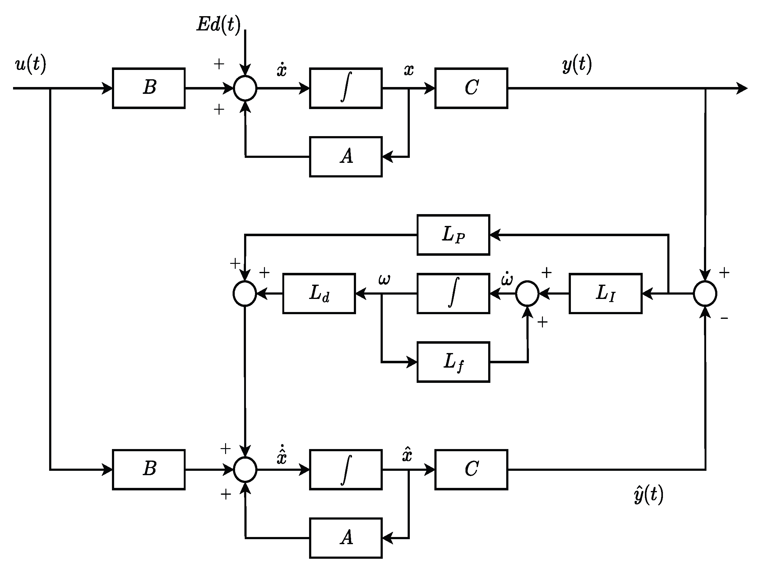
The drawback of PO can be resolved with PIO or GPIO. Depending on the assumptions made for the disturbance, one can either use PIO or GPIO, as will be described in this section. The structure of PIO is a special case of GPIO and will not be separately discussed. GPIO provides complete freedom for the design parameters of the observer and can fit for any desired objectives. So, let us define the GPIO by [
24]
where
represents the integral term and
are the gain matrices defined as the proportional, integral, fading, and direct integral parameter matrices, respectively. The GPIO Equations (
4) and (
5) can compactly be written as
where we dropped the time argument for simplicity of notation and define
with
It is easy to show that the error dynamics of GPIO can be obtained as
where
and the observability of the pair
guarantees that we can obtain
. Note that if the fading term
is eliminated and
, the GPIO reduces to the PIO structure as it was introduced in connection to the LTR design associated with an observer-based LQR [
18]. On the other hand, if one is interested to use GPIO for disturbance estimation and accommodation, then
w is replaced by
and
. In this case, the designer may also use the GPIO without the fading term
or by carefully selecting
, depending on the additional knowledge of the disturbance signal
.
Figure 1 shows the structure of GPIO, when disturbance estimation is of interest.
3.1. GPIO Without Fading Term
Theorem 1. Consider the systems (1), (2) and assume that is a smooth bounded disturbance such that exists. Then there exists a GPIO for the system (1), (2) of the form (4), (5) with , , and such that and , where and if and only if is an observable pair andwhere and with . Proof. Using the statement of the theorem, the GPIO without the fading term becomes a PIO, which is written as
The error dynamics of the state combined with (
10) can easily be constructed as
The eigenvalues of the matrix
can arbitrary be assigned in a stable region of complex planes by the appropriate selection of
and
matrices if and only if the matrix pair
is observable, i.e.,
for all
. This condition is equivalent to
when
, which is the condition 8 of theorem 1, and
for all
when
, which is the observability condition of the pair
. Thus, the dynamical equation (
11) is asymptotically stable and its solution will converge to the equilibrium point, i.e.,
where
. Denoting
and
, we can rewrite the above equation as
and
Since
is the design parameter, we have
, and augmenting it with
yields
Due to the observability of the pair , one can conclude that , or . Substituting it in the first equation, it follows that or . This completes the proof of the theorem. □
Remark 1. Note that for the special case of constant disturbance d, we have and Consequently, the stability of with proper selection of guarantees and .
3.2. GPIO with Fading Term
Theorem 2. Consider the system (1), (2) and assume that is a smooth bounded disturbance. Then there exists a high-gain GPIO for the system (1), (2) of the form (4), (5) with , and such that and , where and if and only if is an observable pair, andwhere ν is the observibility index. Proof. Similar to the Proof of Theorem 1, the GPI observer with the fading term is given by
where
,
, and
, as defined in the statement of the theorem. The error dynamics of the state combined with (
17) can easily be constructed as
The eigenvalues of the matrix
can arbitrary be assigned in the stable region of the complex plane by proper selection of the matrices
and
if and only if the matrix pair
is observable or equivalently, the pair
is observable and the rank condition (
14) is satisfied. The stability of
along with the bounded assumption of
guarantee the solution of (
18) to be bounded. Now, let
and
, then (
18) can be written as
It is easy to see that when
, the above expression reduces to
. Differentiating
and using (
18) we get
Applying condition (
15) and letting
, we get
. Repeating the process of differentiation and using condition (12) leads to
,
. Collecting all the terms, we can write them compactly as
where
can be regarded as the observability index of the pair
. Since the system is observable, it follows that
and its substitution in (
18) gives
. Thus, the stability of
along with conditions (
14), (
15) allow the high-gain GPIO to estimate the states and unknown disturbance as
. □
3.3. Analysis of the Fading Term
A quick derivation reveals that the error dynamics of state and disturbance can be written as
If the unknown input is assumed to be approximated by a fictitious dynamic system with stable matrix F, then the stability of is sufficient for convergence of and . However, when the disturbance is assumed to be bounded, we were able to estimate the disturbance by a high-gain GPIO with a fading term F. Furthermore, an analysis shows that the appropriate selection of F can be used to control the quality of estimation and convergence rate of by moderate-sized observer gains.
Let us write the Laplace transform of (
20) and perform simple algebraic manipulations to obtain
where
and
. To minimize the effect of the unknown input
on the estimation error
in (
22), it is required that
Since the unknown input is assumed to be bounded, the high-gain observer with
will reduce the estimation error
to the extent possible. However, a very high gain may have an undesirable effect on the measurement noise and unmodeled dynamics. The additional fading term
F may be adjusted to avoid unnecessary increases of high gain. It can also be tuned so that the effect of transients on the integral action decays over time. Note that when the bounded disturbance is constant, then
in (
20) and one immediately selects
. Thus, one can apply GPIO without the fading term as in Theorem 1.
4. Power System Model and LFC
4.1. State Space Model
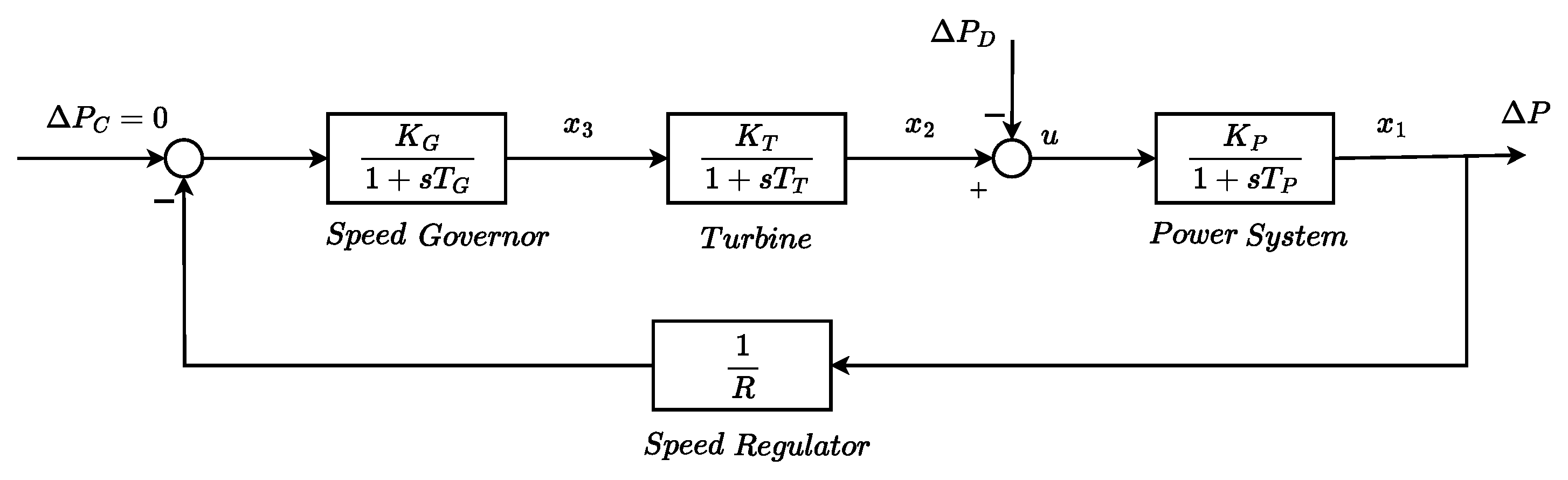
In this section, the case of a single generator supplying power to a single service area is considered. Since for the load frequency control problem the investigated power system is affected by small changes in load, it can be sufficiently represented by the linear model shown in
Figure 2 by linearizing the plant around the operating point [
2,
3].
It is well-known that the load frequency control system consists of four major parts: power system, turbine, governor, and speed regulator, which are defined in
Figure 2.
The associated gains for the first three blocks are and the corresponding time constants are denoted by , respectively. The speed regulator parameter of the governor is specified by R. The load disturbance, the reference input, and the output of the system are , and , respectively. For the purpose of regulation, we consider a free governor operation, i.e., .
Let us define the output of each block by state variables , and . The state represents the frequency variation of the system, the state is the output power of the turbine which is attached to the power generator by a shaft, and the state defines the valve position of the governor, which controls the flow of steam into the turbine.
Using the transfer functions associated with each block, defining the state variables
, and
, and assuming
, one can write the state equation of the system as follows
For the purpose of comparison with previous results we consider the typical values for parameters used in for the LFC model [
3,
18]. The third-order model defined in (
23) can be extended to a fourth-order model by considering an integral action on the state of frequency variation
, i.e.,
. This leads to the following state space representation
with
.
4.2. State Feedback Design of LFC
The power flow from the generator passes through several stations, which are connected by transmission lines. Frequency variation usually propagates in this process and affects the smooth operation of power systems. Load frequency control
is a proper procedure to maintain the frequency deviation within an acceptable tolerance. Applying the state feedback control law
to (
23), the characteristic equation of the closed-loop system can easily be derived and represented by a cubic equation
. The coefficients
, and
are given in terms of the known parameters and the feedback gains
, and
. One way to design the control law is to apply the Hurwitz stability condition and obtain the feasible solution to ensure stability and possibly to improve the performance. However, the procedure is not systematic and a more reliable approach is to apply optimal control using LQR. Nevertheless, let us obtain the allowable range of feedback gains for stability of the third-order system (
22). The necessary and sufficient condition for stability in terms of
,
, and
are
,
, and
, where
Using the numerical values defined for the third-order system (
23), the range for the stability of the controllable gains can be obtained as
,
, and
. If one considers the gravitational search algorithm (GSA) proposed in [
25], one can obtain
,
, and
with respect to the objective function defined for GSA.
On the other hand, if LQR is applied with the performance index
the feedback gain is given by
where
P is the solution of the algebraic Riccati equation
and
are the positive definite weighting matrices.
5. Disturbance Accommodation with GPI Observer-Based Controller
The problem of LFC becomes even more challenging when unknown disturbances are present and may cause undesirable effects on the performance of power systems. In addition, most available results on LFC assume that all states of the system are available for measurement. However, due to a number of reasons, such as physical constraints, sensor placement, and cost, it is desirable to use observers to estimate the states of power systems. Unfortunately, the conventional proportional observer (PO) cannot be used if unknown disturbances are incorporated in the system, as we elaborated in the introduction. Consequently, we provided the complete development of a generalized proportional integral observer (GPIO), which can reliably be an observer-based LFC.
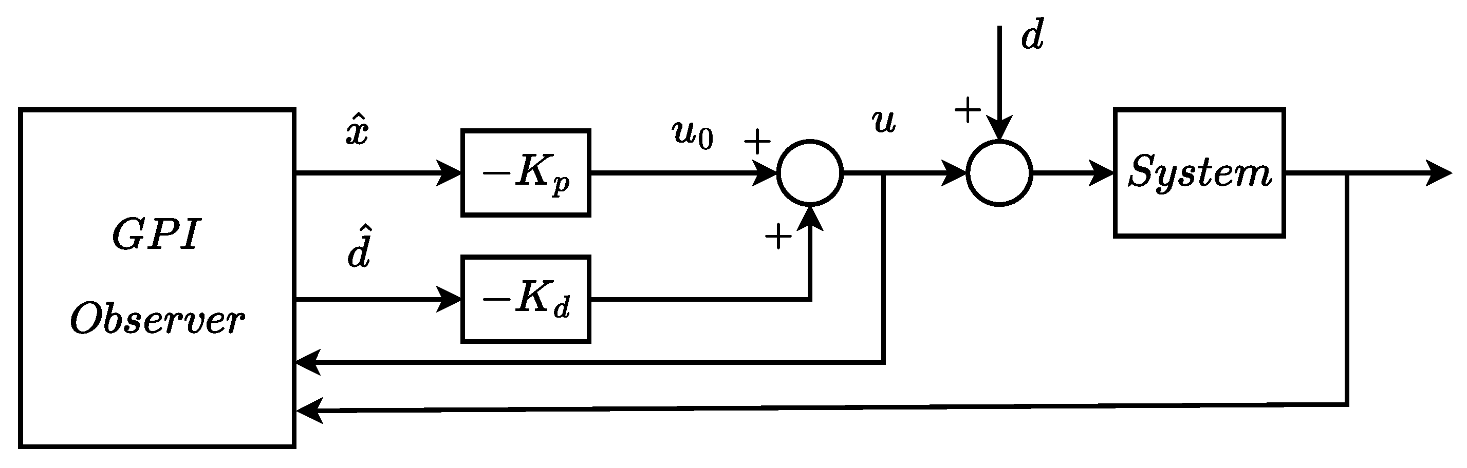
Since the GPIO is estimating both states and unknown disturbance, an indirect approach for disturbance accommodation is based on the equivalent input disturbance cancellation. To illustrate this approach, let us assume for simplicity that
in
Figure 1 and applying the state feedback control law
to
, as shown in the simplified
Figure 3.
In the following, we provide a direct approach to disturbance accommodation using GPIO-based optimal control.
GPIO-Based Controller
Applying the state feedback control law
to the systems (
1), (
2) and the GPIOs (
4), (
5), as specified in
Figure 1, we obtain the combined control loop system
where we used the parameters of GPIO with
,
, and
. If we define
and
, the first equation of (
30) leads to
Suppose
, which requires
, then
and (
30) reduces to
Equation (
33) clearly shows the separation property of the GPIO-based state feedback controller. Consequently, the eigenvalues of the composite matrix in (
33) is the union of those in
and those of the GPIO eigenvalues, as is evident from (
20). According to Theorem 1 or Theorem 2, the steady-state estimation errors approach zero, i.e.,
and
. Therefore, the effect of the error in (
33), or equivalently in (
31), can be neglected and we have the closed loop system.
where we eliminated the reference variable, i.e.,
. What remains to be done is to design the state feedback
, such that (
34) is asymptotically stable and minimizes the quadratic performance index (
26). Choosing the Lyapunov function as
and using standard techniques, one can guarantee stability and satisfy the following upper bound of the performance index
if the following inequality holds
Furthermore, in order to find the minimal cost function, we may minimize , where is required, i.e., .
Theorem 3. System (34) is asymptotically stable satisfying the cost control performance index (36), if the following LMI is feasible with variables X and Y:where and the state feedback gain can be obtained as . Proof. Multiplying (
37) on the left and right by
and applying the Schur complement formula, one can establish the equivalence of (
37) and (
38). The equivalence of (
39) and
can also be verified again by the Schur complement formula, i.e., for a symmetric matrix
M partitioned as
if and only if
. So, by defining
,
, and
, (
39) reduces to
. □
Remark 2. If the condition , i.e., is not satisfied, we can still apply the procedure by imposing the condition , which is equivalent to a least square solution for .
6. Simulation Results
The simulation results for the power system described in
Section 4 using the disturbance accommodation techniques introduced in
Section 5 are presented here. For a better comparison between the discussed methods, the LFC for the power system model described in
Section 4 is studied using Luenberger, PI, and GPI observers.
In this study, we used typical values of the power system parameters [
3,
18]:
, , , , , s, and .
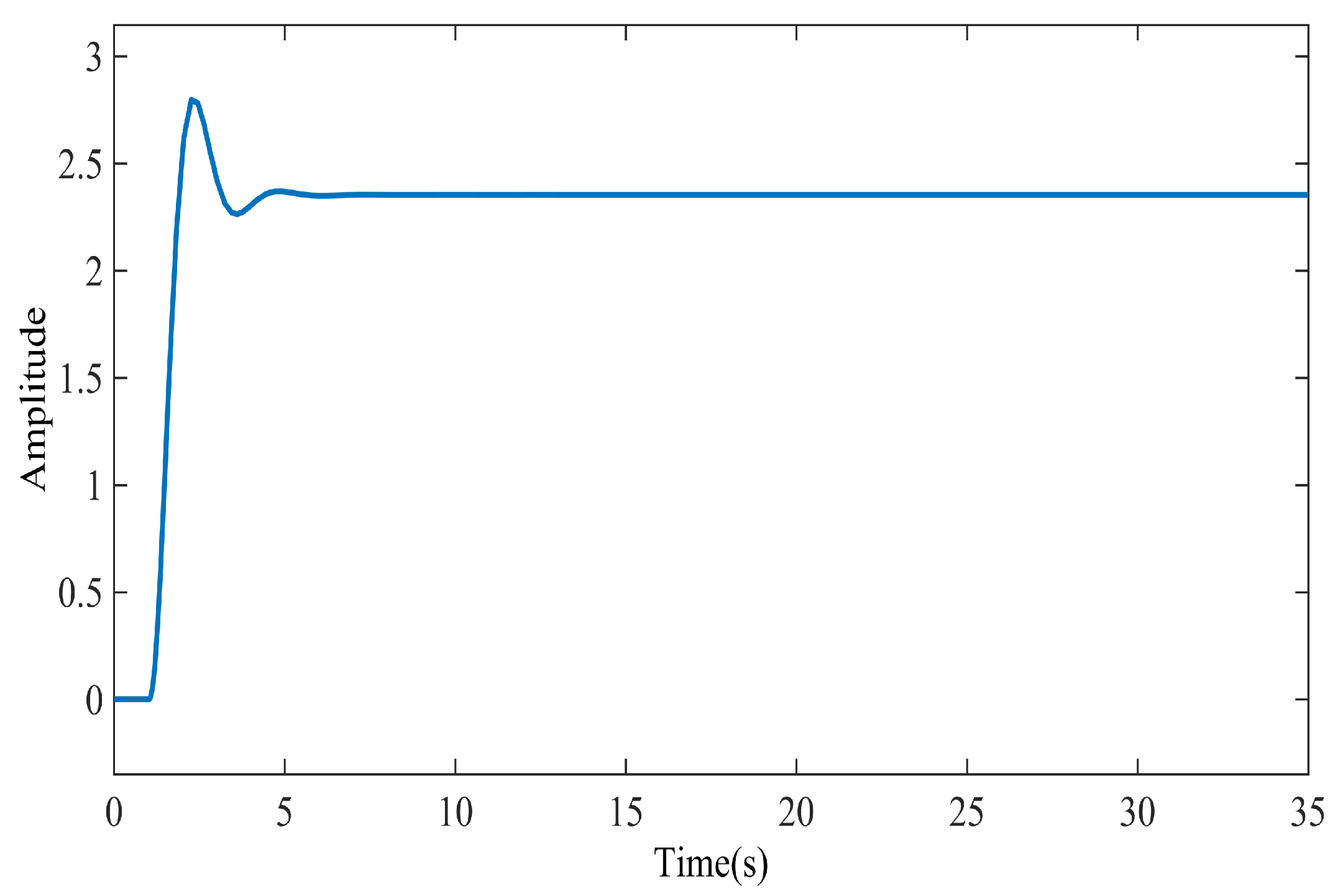
Figure 4 shows the step response for the power system discussed in
Section 4, in which the under damped property of the model is apparent.
6.1. Performance of the Proposed Control Strategy for LFC
Proportional, PI, and GPI observers are developed for the single-area power system modeled in
Section 4 using the following values determined via pole placement:
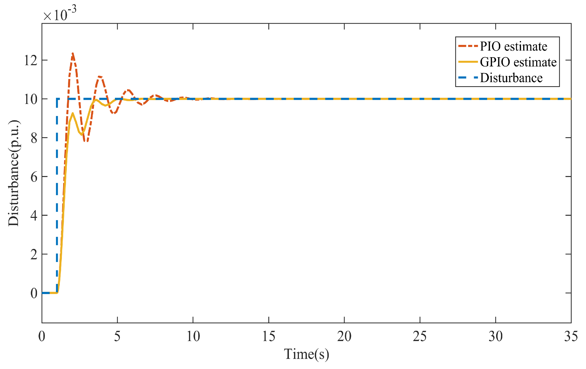
The disturbance is considered to be a step function of value p.u. and is injected into the system at . For an optimal observer design, the gain should be calculated in such a way that the error dynamics should regulate to zero.
The results of disturbance estimation and LFC using PO, PI, and GPI observers are presented in
Figure 5 and
Figure 6, and
Table 1 presents the numerical values of the maximum frequency deviation and the corresponding settling time, defined as the time required for
to enter and remain within a 0.005 Hz bound.
While the conventional Luenberger observer is not able to estimate the disturbance, it is evident in
Figure 5 that the GPIO estimates disturbances more quickly and with less overshoot compared to the PIO, attributed to the incorporation of the additional fading term in the GPIO framework. Consequently, the output frequency of the system demonstrates reduced overshoot and improved settling time, as shown in
Figure 6.
6.2. Disturbance Estimation
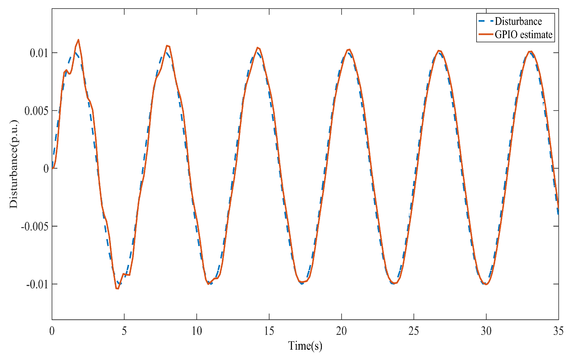
To further evaluate the effectiveness of the proposed method in estimating unknown disturbances, in this section, two additional scenarios involving more complex disturbance profiles are examined: first, a sinusoidal disturbance with an amplitude of p.u. and a frequency of 1 Hz is injected into the system at s and second, a combination of step functions with various magnitudes is applied at different time instances.
As shown in
Figure 7 and
Figure 8, the GPI observer is able to successfully estimate these disturbances. The results demonstrate that the proposed method is capable of accurately estimating complex forms of dynamic disturbances without requiring any prior knowledge about their nature.
While the GPIO-based LFC results presented in this section demonstrate robust performance across the considered scenarios, its effectiveness may be limited under certain practical conditions such as substantial modeling inaccuracies, nonlinear dynamics, or high measurement noise levels. These factors may affect the accuracy of disturbance estimation and observer convergence.
7. Conclusions
In this paper, a proportional integral observer (PIO) and its generalization (GPIO) are introduced for the load frequency control (LFC) of a single-area power system. This study demonstrates that the GPI observer can improve the LFC of the system in certain aspects such as reducing the maximum deviation of the system frequency from its nominal value and decreasing the settling time. Since GPIO is able to estimate both the states and unknown disturbances, it can be integrated in LFC with disturbance accommodation to ensure the system stability and to satisfy the specified performance measures. Specifically, by understanding the form of disturbance in power systems using GPIO, a more effective decision-making, enhancement of the system’s reliability, and contribution to the overall resilience of power systems becomes feasible. Future work will aim to improve the robustness of the observer under challenging conditions, including significant model uncertainties, nonlinear system behavior, and high levels of measurement noise. Additionally, adaptive and nonlinear extensions of the proposed approach will be investigated to enhance its applicability in more complex scenarios.


