Flexible Demand Side Management in Smart Cities: Integrating Diverse User Profiles and Multiple Objectives

Abstract

Demand Side Management (DSM) plays a crucial role in modern energy systems, enabling more efficient use of energy resources and contributing to the sustainability of the power grid. This study examines DSM strategies within a multi-environment context encompassing residential, commercial, and industrial sectors, with a focus on diverse appliance types that exhibit distinct operational characteristics and user preferences. Initially, a single-objective optimization approach using Genetic Algorithms (GAs) is employed to minimize the total energy cost under a real Time-of-Use (ToU) pricing scheme. This heuristic method allows for the effective scheduling of appliance operations while factoring in their unique characteristics such as power consumption, usage duration, and user-defined operational flexibility. This study extends the optimization problem to a multi-objective framework that incorporates the minimization of CO₂ emissions under a real annual energy mix while also accounting for user discomfort. The Non-dominated Sorting Genetic Algorithm II (NSGA-II) is utilized for this purpose, providing a Pareto-optimal set of solutions that balances these competing objectives. The inclusion of multiple objectives ensures a comprehensive assessment of DSM strategies, aiming to reduce environmental impact and enhance user satisfaction. Additionally, this study monitors the Peak-to-Average Ratio (PAR) to evaluate the impact of DSM strategies on load balancing and grid stability. It also analyzes the impact of considering different periods of the year with the associated ToU hourly schedule and CO₂ emissions hourly profile. A key innovation of this research is the integration of detailed, category-specific metrics that enable the disaggregation of costs, emissions, and user discomfort across residential, commercial, and industrial appliances. This granularity enables stakeholders to implement tailored strategies that align with specific operational goals and regulatory compliance. Also, the emphasis on a user discomfort indicator allows us to explore the flexibility available in such DSM mechanisms. The results demonstrate the effectiveness of the proposed multi-objective optimization approach in achieving significant cost savings that may reach 20% for industrial applications, while the order of magnitude of the trade-offs involved in terms of emissions reduction, improvement in discomfort, and PAR reduction is quantified for different frameworks. The outcomes not only underscore the efficacy of applying advanced optimization frameworks to real-world problems but also point to pathways for future research in smart energy management. This comprehensive analysis highlights the potential of advanced DSM techniques to enhance the sustainability and resilience of energy systems while also offering valuable policy implications.

1. Introduction

In recent years, the growing emphasis on energy efficiency and the rising importance of renewable energy sources has led to an increased focus on the optimization of electrical power consumption [1,2]. This is particularly pertinent in the context of Demand Side Management (DSM), which plays a critical role in modern energy systems by aligning consumer energy usage with supply conditions. DSM not only facilitates significant cost reductions and enhances the reliability of power systems but also contributes to the overarching goal of reducing carbon footprints. As the penetration of renewable energy sources increases, the flexibility that DSM offers becomes crucial in managing the variability associated with these sources.

The advancement of smart grid technologies has paved the way for a new era of possibilities for DSM [3]. Smart grids integrate various digital information and communication technologies into traditional power networks, enabling real-time monitoring and management of energy flows. This integration helps in optimizing the production and distribution of electricity and revolutionizes the way that energy is used and saved [4,5]. Smart cities can leverage smart grid developments to manage the load profiles of their diverse and complex mix of residential, commercial, and industrial consumers [5,6].

Very often the management of load in a smart city is performed with the aim of addressing one particular objective function, such as minimization of cost for its consumers, minimization of CO₂ emissions, or minimization of Peak-to-Average Ratio (PAR) load in the grid (aiming at improving grid resilience). Recent approaches increasingly try to address a combination of those and other objective functions [7,8,9,10,11], mindful of multiple stakeholders and technical and societal concerns [12]. In particular, most early studies did not explicitly consider the impact of the load shifting on consumers, especially regarding discomfort or business implications. Consumer discomfort is mostly considered from a thermal point of view or appliance availability, often considering single environment settings (e.g., residential or industrial), and usually in relation to particular optimization objectives [13,14,15,16]. As a result, the benefits proposed by these studies may not be sufficiently realistic [17,18,19].

Heuristic-based approaches emerged as powerful tools in optimization due to the increasing complexity and scale of real-world problems, which often render traditional exact methods impractical or infeasible [20]. Traditional optimization techniques, such as linear programming or gradient descent, rely on precise mathematical formulations and assumptions. These methods can become computationally expensive and inefficient when dealing with large-scale, high-dimensional, or non-linear problems with numerous local optima. Heuristic approaches, inspired by natural processes such as evolution, swarm behavior, and annealing, provide flexible, adaptive, and robust strategies for exploring complex search spaces. They are also frequently used when objective functions or/and constraints of the problem are non-linear. They do not guarantee an optimal solution but can find good-enough solutions within reasonable time frames, making them particularly suitable for problems where obtaining an exact solution is less critical than finding a feasible and satisfactory one. This adaptability and efficiency in handling diverse and intricate problems have driven the widespread adoption and development of heuristic-based optimization methods.

This paper delves into the application of heuristics optimization such as a GA and NSGA-II within a DSM framework, categorizing solutions across residential, commercial, and industrial sectors, with a large number of appliances and distinct constraints. Reasons for using a GA include its widespread use in the energy domain, being simple and robust in this type of problem, and easily handling the existing constraints. The Non-dominated Sorting Genetic Algorithm II (NSGA-II) is a potent tool in this domain, addressing the multi-objective optimization of scheduling electrical appliances to minimize cost, reduce CO₂ emissions, and alleviate user discomfort simultaneously. NSGA-II preserves trade-off by finding a Pareto front of optimal solutions, eliminating the need to aggregate objectives into a single one and thereby avoiding arbitrary weighting. This study highlights the algorithm’s efficacy in navigating the complex trade-offs between competing objectives and underscores the practical implications of such optimizations in real-world settings. Furthermore, it allows for the comparison of results against a single-objective approach where only one objective function (cost) is minimized at the expense of other objective functions (CO₂ emissions, user discomfort, Peak-to-Average Ratio). It is, however, more computationally intensive and requires post-analysis to select adequate solutions from the Pareto front.

In the context of DSM, it is also important to consider the hourly profile of pricing schemes and CO₂ emissions when addressing objective functions aimed at minimizing costs or emissions. Indeed, most pricing schemes vary depending on the year period (e.g., summer vs. winter), and hourly CO₂ emissions depend on the generation mix offered to the load, which also varies seasonally.

The focus of this paper is on the intersection of the following aspects:

• Smart city context with multiple user profiles (with analysis of differentiated impact of DSM in the different profiles);
• The consideration of multiple objective optimization (cost reduction, emissions reduction, discomfort reduction) given the increasing interest and importance of optimizing solutions, taking into consideration multiple aspects, and comparison with single objective optimization, for the evaluation of Demand Side Management;
• Analysis of the impact of seasonality and annual generation mixes on the optimal outcomes of Demand Side Management;
• The use of real data (electricity prices, Time-of-Use profiles, emissions annual profile, device characteristics);
• Extraction of insights for decision-makers with different preferences, including policy, such as the design of Time-of-Use profiles.

The focus is on demonstrating the usefulness of heuristics optimization, rather than advancing existing algorithms (such as the GA and NSGA-II). In this context, analyzing the performance of the energy system across different sectors and periods provides insights into specific challenges and opportunities, offering a comprehensive overview of the strategic application of DSM to enhance energy efficiency and inform potential policy measures.

2. Demand Side Management Techniques

Demand Side Management (DSM) encompasses a range of techniques aimed at encouraging consumers to modify their level and pattern of electricity usage [16]. The primary goal of DSM is to optimize energy consumption and improve the overall efficiency of the electrical grid. The main techniques of DSM can be broadly classified into the following categories of impact:

• Energy Efficiency: This involves measures that lead to a reduction in the energy used by specific end-use devices and systems, without affecting the services provided. These measures include high-efficiency appliances, improved insulation, and more efficient heating and cooling systems. Energy efficiency programs are cost-effective over time, reducing energy consumption and utility bills.
• Load Shifting: Also frequently known as demand response, this technique encourages consumers to increase or decrease their electricity use during specific periods where energy demand is high or when renewable energy availability is high. Load shifting helps in managing the load curve, reducing the need for peak power plants, and enhancing grid reliability. Technologies such as smart thermostats and appliances capable of responding to signals from energy providers to delay or advance their operation time are central to this strategy.
• Peak Load Reduction: This strategy involves programs designed to cut down energy use during peak demand times, such as on hot summer days. Techniques include offering incentives for reduced consumption and temporary increases in electricity prices during peak periods (Time-of-Use pricing).
• Load Filling: Load filling promotes increased energy usage during periods of low demand to maintain consistent electricity production levels. This technique is particularly relevant in systems with high levels of renewable energy generation, where excess energy can be used more effectively.
• Energy Conservation: Broad programs aimed at promoting a culture of energy savings among consumers through behavioral change. Education and information dissemination play key roles in these programs, encouraging sustained energy-saving habits.
• Integrated DSM: This approach combines several DSM strategies to achieve optimal energy savings. For instance, integrating real-time energy monitoring tools with consumer incentives and education can lead to more significant energy savings and operational efficiencies.

DSM techniques are instrumental in stabilizing the grid and making energy use more sustainable and cost-effective. The implementation of DSM can vary significantly depending on regional regulatory policies, the maturity of the local energy market, and consumer engagement levels. In the present study, load shifting was considered.

3. Problem Formulation and Algorithm Description

3.1. Problem Formulation

The problem under study addresses the optimization of electrical appliance scheduling within residential, commercial, and industrial sectors. This section provides a detailed formulation of the variables, objective functions considered throughout this work, and constraints involved, for the implementation of the GA and NSGA-II.

A. Variables:

$g=\left(a,s,d\right)$: Represents a gene in the chromosome, where

$a$: Appliance identifier.

$s$: Start time of the appliance’s operation within a 24 h period.

$d$: Duration of the appliance’s operation.

A chromosome is composed of sequences of genes; thus, it has as many genes as appliances in the considered problem.

B. Objective Functions:

• Cost ($\mathrm{C}$) Minimization:

$$C={\sum }_{h=0}^{23}\left({\sum }_{g\in G}{P}_g\times I_{g,h}\right)\times E_h$$

(1)

where $P_g$ is the power consumption of the appliance in gene $g$, $I_{g,h}$ indicates if the appliance in gene $g$ operates during hour $h$, $G$ is the set of all genes, and $E_h$ is the electricity price at hour $h$.

2.

Discomfort $\left(D\right)$ Minimization:

$$D={\sum }_{g\in G}\left|s_g- s_{g,pref}\right|\times {\delta }_g,$$

(2)

where $s_g$ is the effective start time (hour) for the appliance in gene $g$, $s_{g,pref}$ is the preferred start time (hour) for the appliance in gene $g$, and ${\delta }_g$ is the hourly discomfort penalty associated with the appliance in gene $g$.

3.

CO₂ Emission $\left(E\right)$ Minimization:

$$E={\sum }_{h=0}^{23}\left.\left({\sum }_{g\in G}{P}_g\times I_{g,h}\right.\right)\times X_h,$$

(3)

where $X_h$ represents the CO₂ emission factor at hour $h$.

C. Constraints:

• Power Constraint: Ensures that the power consumed at any hour does not exceed the maximum allowable limit:

$$\forall h\in \{0,\dots ,23\},{\sum }_{g\in G}{P}_g\times I_{g,h}\le L_{max},$$

(4)

where $L_{max}$ the peak power limit.

From the implementation point of view, this restriction can be included in the cost function with the following additional term:

$${\sum }_{h=0}^{23}max{\left(0,L_h-L_{max}\right)}^2,$$

(5)

where $L_h$ is the total load at hour $h$.

ii.

Operational Constraints: Each appliance must adhere to its operational limits regarding minimum and maximum usage durations and daily usage frequency.

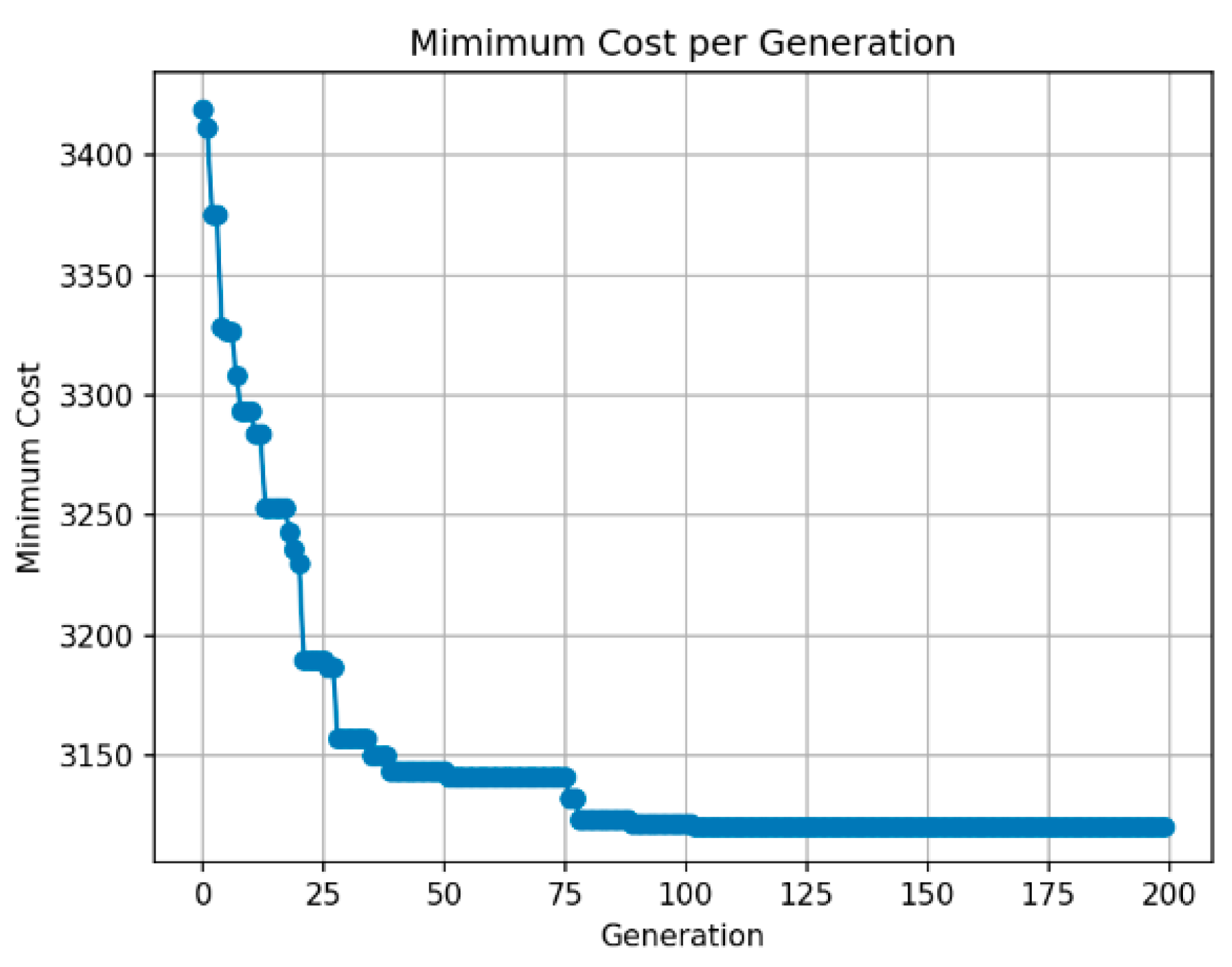
3.2. Algorithm Description

• Genetic Algorithm (GA)

A Genetic Algorithm, developed in Python, version 3.12.2, is used to search for optimal solutions for the single-objective problem of minimizing the cost function. It is a heuristic optimization technique inspired by the principles of natural selection and genetics. It is used to find approximate solutions to complex optimization problems by iteratively improving a population of candidate solutions. The main components of a GA include selection and tournament, crossover (recombination), mutation, and elitism. These components are used to explore the search space and exploit the best solutions found during the search process.

The population size determines the number of individuals (candidate solutions) in the population. A larger population size increases the diversity of solutions but also requires more computational resources.

The crossover rate is the probability with which crossover (recombination) occurs between pairs of individuals to create offspring. A higher crossover rate promotes the exchange of genetic material, leading to greater exploration of the search space. A uniform crossover mechanism allows genes (appliance schedules) from parent chromosomes to mix, promoting variability in the offspring.

The mutation rate refers to the probability of introducing random mutations into individuals within a population. A higher mutation rate increases diversity and helps prevent premature convergence in local optima but can also disrupt good solutions.

The number of generations is the number of iterations the algorithm will run. More generations allow the algorithm to refine solutions further but require more computational time.

The selection mechanism is the method used to select individuals for reproduction based on their fitness. Common mechanisms include tournament selection and roulette wheel selection. They influence the algorithm’s convergence rate and diversity. In our case we applied a tournament selection process.

Elitism aims at ensuring that the best solutions are carried over to the next generation. It preserves high-quality solutions and helps maintain the best-found solutions throughout the evolutionary process.

In our study the following parameters were used in the Genetic Algorithm (GA), based on multiple tests using different combinations of parameters:

• Population Size: 400;
• Number of Generations: 100;
• Crossover Probability: 0.9 (random single point);
• Mutation Probability: 0.1;
• Tournament size: 3;
• Elite Size: 10.

The stopping criteria for the algorithm was the total number of generations (200), thus limiting the maximum amount of time that the algorithm would run.

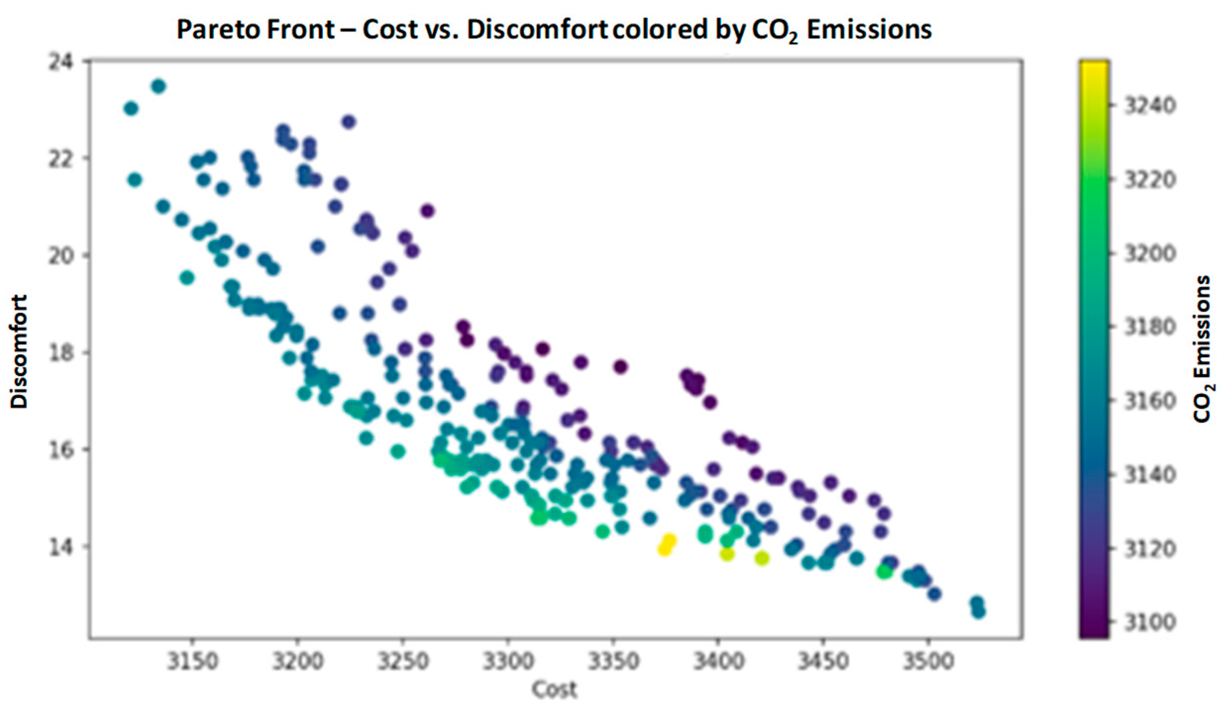
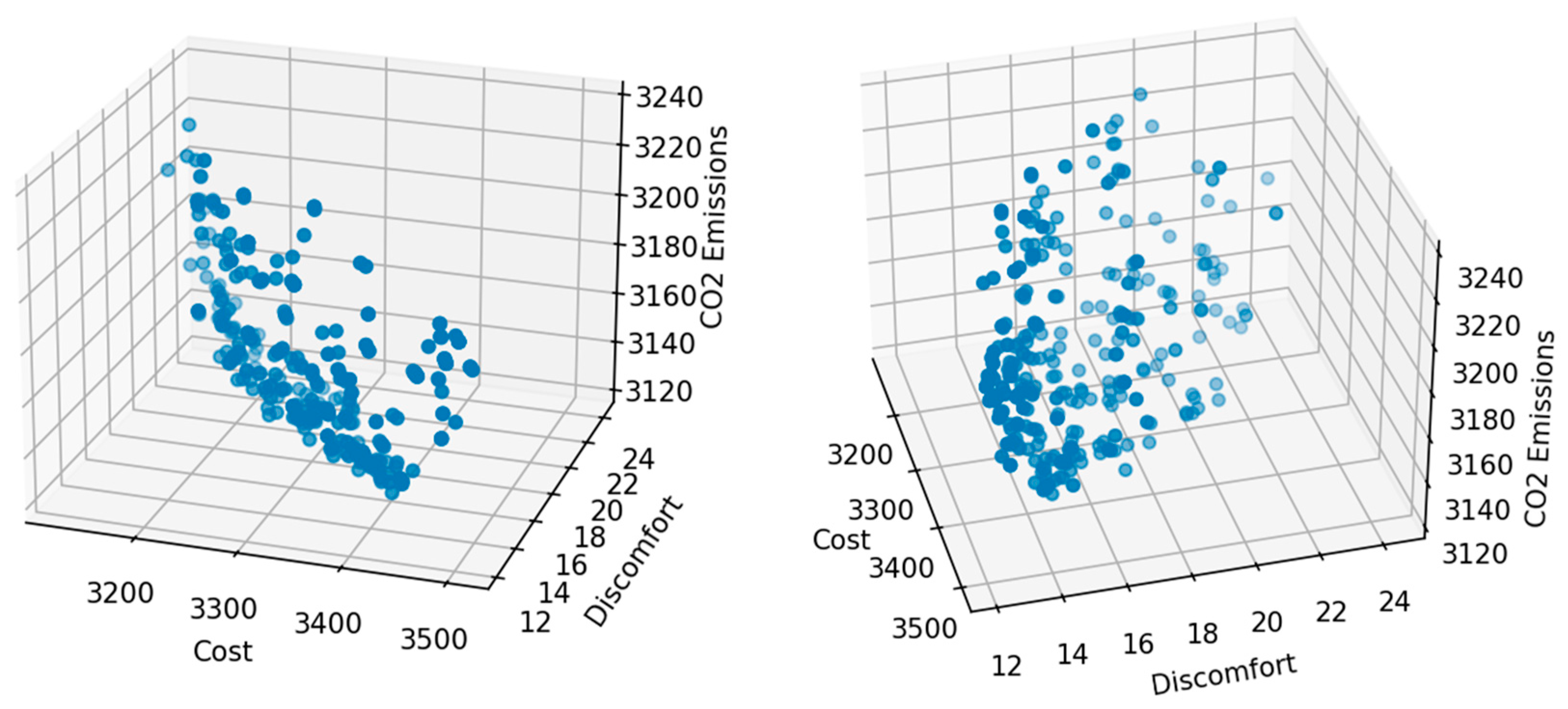
B.

Non-Dominated Sorting Genetic Algorithm II (NSGA-II)

The Non-dominated Sorting Genetic Algorithm II (NSGA-II) [21] is an advanced multi-objective optimization algorithm that extends the principles of GAs to handle multiple objectives. NSGA-II aims to find a set of Pareto-optimal solutions, where no single solution is strictly better than another across all objectives. It uses mechanisms like non-dominated sorting, crowding distance, and elitism to ensure diversity and convergence to the Pareto front.

The selection mechanism selects individuals for reproduction based on their rank and crowding distance, thus balancing convergence and diversity by preferring non-dominated individuals and maintaining spread.

The crowding distance provides a measure of the density of solutions surrounding a particular solution in the objective space. This ensures diversity by preserving a spread of solutions across the Pareto front.

The non-dominated sorting mechanism classifies individuals into different fronts based on Pareto dominance. This helps identify and rank solutions based on their dominance, facilitating multi-objective optimization.

In our study the following parameters were used in the NSGA-II algorithm, also developed in Python, based on multiple tests using different combinations of parameters:

• Population Size: 400;
• Number of Generations: 100;
• Crossover Probability: 0.9 (random single point);
• Mutation Probability: 0.1.

The stopping criteria considered were the same as for the GA.

4. Scenario and Model Specification

4.1. Scenario Details

The scenario was designed to reflect realistic household, commercial, and industrial environments in the context of a smart grid for a smart city where energy consumption optimization is crucial. This study evaluates a mixed residential, commercial, and industrial setting with the following characteristics:

• Residential Sector: Includes common appliances like refrigerators, washing machines, dryers, and ovens. Each appliance has varying power requirements, preferred operational times, and flexibility in operation, reflecting typical household energy consumption patterns.
• Commercial Sector: Focuses on energy-intensive appliances like water dispensers, ovens, and air conditioning units commonly found in office buildings and small businesses. These appliances typically have less flexibility in operation times but contribute significantly to the energy footprint of commercial establishments.
• Industrial Sector: Comprises heavy machinery such as water heaters, welding machines, and induction motors. These units are high-power consumers with strict operational schedules to maintain industrial productivity.

This study uses hourly electricity pricing and CO₂ emissions factors that vary throughout the day, reflecting the dynamic nature of energy markets and environmental impacts associated with electricity generation. Furthermore, different periods of the year are considered to account for distinct daily hourly profiles for energy prices and for CO₂ emissions. The optimization aims to balance cost, discomfort, and emissions, providing a comprehensive strategy for DSM in mixed-use environments.

4.2. Appliance Characterization

Appliances across the three sectors are characterized by their power requirements, operational timings, flexibility, and user-defined preferences. Realistic data was collected from the literature [22,23,24,25] to reflect the characteristics of a smart city. Each appliance type is detailed in the tables below, including their rated power (in W), minimum and maximum usage durations (in hours), maximum daily usage, preferred start time (between hour 1 and hour 23), start time flexibility (in number of hours), discomfort penalty (an integer index), and quantity. The “start time” is the moment of the day when it is expected to start using such an appliance. The “start time flexibility” represents the number of hours that such a starting moment is allowed to be anticipated or delayed. For example, a dish washer or a washing machine could in principle operate any time of the day; therefore, a 24 h “start time flexibility” is assigned. A toaster or a TV would in principle be used at a certain time of the day, hence a value of 1. Appliances that are non-controllable or are not allowed to have starting time flexibility have a starting time flexibility value of 0 (zero). As indicated in the study of [26], commercial loads offer more limited flexibility than residential due to the prioritization of occupant comfort and safety, and maintaining business operations, over energy savings, and the flexibility of industrial electricity demand is recognized as being considerably lower, due to technical constraints and greater immediate negative costs for stoppages or reductions, than for other sectors. For these reasons, the starting time flexibility is higher in most residential appliances than in commercial ones and higher in commercial appliances than in industrial ones [27]. This is also in line with empirical appliance utilization scheduling tables [25,28], constraints in appliance usage [26,29], and starting times, end times, and usage duration of appliances [25,30,31]. Accordingly, the discomfort penalty was considered to be between 1 and 2 for Residential appliances, 5 for Commercial appliances, and 10 for Industrial appliances in order to reflect a lower ability to move schedules in commercial and industrial environments. As mentioned in Section 1 above, most of the discomfort quantification approaches in the literature address it from either the thermal or waiting times points of view [32,33,34], which, although allowing for a detailed and complex analysis of some appliances’ behavior, do not capture the complete range of discomfort reasons in the residential, commercial, and industrial settings in a uniform manner (e.g., rescheduling of staff, ability to anticipate use, operational restrictions or implications). The discomfort penalty allows for encompassing several factors, in a uniform way and simplified manner, at the cost of more detail. Together with the “start time flexibility”, it can be used as a proxy for the concept of “flexibility”. By modifying the discomfort penalty values and flexibility ranges, the present framework can be adjusted for different cities’ characteristics, according to the type of industry present, the type of existing commercial and service buildings, and the characterization of the residential framework. This allows us to study the flexibility associated with different city settings. The fine tuning of the discomfort penalty values used and the consequent impact on metrics of the characteristics of different cities deserves dedicated consideration and is out of the scope of the present paper and is planned to be studied in follow-up research.

We have considered a total of 4621 appliances, with 3704 residential appliances across 17 appliance types, 808 commercial appliances across 9 appliance types, and 109 industrial appliances across 9 appliance types. These correspond to an amount of nominal power of the same order of magnitude for the different categories (2.88 MW for residential, 2.38 MW for commercial, and 3.64 MW for industrial).

Table 1. Residential appliances.

Appliance	Power (W)	Min Duration (h)	Max Duration (h)	Preferred Start Time (h)	Start Time Flexibility (h)	Discomfort Penalty	Quantity
Dryer	1200	1	1	21	24	1	189
Dish washer	700	1	2	21	24	1	288
Washing machine	500	1	2	21	24	1	268
Oven	1300	1	1	19	3	2	279
Iron	1000	1	1	18	10	1	340
Vacuum cleaner	400	1	1	11	10	1	158
Fan	200	2	5	13	5	1	288
Kettle	2000	1	1	17	2	1	406
Toaster	900	1	1	8	1	1	48
Rice cooker	850	1	1	19	3	2	59
Hair dryer	1500	1	1	8	1	1	58
Blender	300	1	1	17	10	1	66
Frying pan	1100	1	1	19	3	2	101
Coffee maker	800	1	1	8	1	2	56
Tv	300	2	4	20	1	1	300
Lights	200	3	6	19	1	2	400
Continuous loads	400	24	24	0	0	2	400

,

Table 2. Commercial appliances.

Appliance	Power (W)	Min Duration (h)	Max Duration (h)	Preferred Start Time (h)	Start Time Flexibility (h)	Discomfort Penalty	Quantity
Water dispenser am	2500	5	7	11	3	5	78
Water dispenser pm	2500	5	7	16	3	5	78
Dryer	3500	4	6	11	3	5	117
Kettle	3000	2	3	16	3	5	123
Oven	5000	1	2	13	2	5	77
Coffee maker	2000	2	3	13	2	5	99
AC/fan	3000	2	3	14	3	5	93
AC	3500	3	3	14	3	5	56
Lights	1750	24	24	0	0	5	87

and

Table 3. Industrial appliances.

Appliance	Power (W)	Min Duration (h)	Max Duration (h)	Preferred Start Time (h)	Start Time Flexibility (h)	Discomfort Penalty	Quantity
water heater	12,500	3	5	10	3	10	39
welding machine	25,000	5	5	9	1	10	35
fan/AC	30,000	5	6	11	2	10	16
arc furnace	50,000	6	7	9	2	10	8
induction motor	100,000	6	6	9	2	10	5
dc motor am	150,000	3	4	9	2	10	3
dc motor pm	150,000	3	4	15	2	10	3

below list the appliances, their quantities, and characteristics. Figure 1 depicts the load profile of the commercial setting without DSM activated.

4.3. Pricing Schemes

The scenario adopted employs a Time-of-Use electricity pricing considering real-world conditions. The ToU scheme varies throughout the day, with higher prices during peak demand periods and lower prices during off-peak times, encouraging load shifting. Real values from existing commercial offers in Portugal were considered [35]. Since, in the country, ToU presents different periods in summer and in winter, two sets of pricing schemes were considered where the ToU blocks are distributed through different hours of the day, as per the national regulator [36]. Although these data are specific to Portugal, they reflect a common practice in Europe, therefore making the results realistic to wider geographies.

The Time-of-Use Pricing values are the following (EUR/kWh):

• Peak Hours: 0.30;
• Mid-Peak Hours: 0.18;
• Off-Peak Hours: 0.15;
• Super Off-Peak Hours: 0.11.

Table 4. Daily pricing profile (EUR/kWh).

Hour		0	1	2	3	4	5	6	7	8	9	10	11
Price	Summer	0.15	0.15	0.11	0.11	0.11	0.11	0.15	0.15	0.18	0.18	0.18	0.3
	Winter	0.15	0.15	0.11	0.11	0.11	0.11	0.15	0.15	0.18	0.3	0.3	0.18
Hour		12	13	14	15	16	17	18	19	20	21	22	23
Price	Summer	0.3	0.18	0.18	0.18	0.18	0.18	0.18	0.18	0.3	0.18	0.15	0.15
	Winter	0.18	0.18	0.18	0.18	0.18	0.18	0.3	0.3	0.3	0.18	0.15	0.15

presents the daily pricing profile.

4.4. CO₂ Emissions

CO₂ emission factors vary on an hourly basis, reflecting the changing environmental impact of electricity generation throughout the day [37]. These factors are essential for quantifying the carbon footprint associated with appliance operation schedules. In this study, real data from Portugal’s 2023 generation mix was used, based on publicly available information from the national system operator (REN) [38]. The data, originally provided at 15 min intervals, was aggregated to an hourly resolution to enable analysis of the hourly emission profile. Emission factors specific to each generation source were considered for the Portuguese context [39,40]. With this data, an hourly profile of carbon intensity in consumption was generated. Portugal has a high penetration of renewable energy in its electricity mix, with more than 61% of demand met by renewables in 2023. As the generation mix fluctuates both daily and seasonally, CO₂ emissions vary accordingly. Therefore, it is essential to consider multiple days when evaluating the impact of Demand Side Management (DSM) on CO₂ emissions under varying generation conditions. In this study, five distinct days were analyzed based on their specific characteristics, as detailed in

Table 5. Periods analyzed.

Period	Date	Characterization
0	6 July 2023	Summer sunny	41% RES
1	30 January 2023	Winter sunny	62% RES
2	10 January 2023	Winter wet/natural gas	70% RES
3	10 September 2023	Low RES (annual minimum)	21% RES
4	11 November 2023	High RES (annual maximum)	85% RES

and

Table 6. CO₂ emissions daily profiles (hourly CO₂ emission factors—g CO₂ eq/kWh).

Hour	Period
	0	1	2	3	4
0	221.6	67.9	77.6	162.9	29.8
1	231	68.5	74.5	179.5	31.3
2	233.2	63.8	73	189.7	33.9
3	234.3	75.3	79.9	195.1	34.9
4	240.5	90	84	196.9	33.9
5	210.8	103.6	84.2	196	32
6	185.9	94.9	87.7	178.6	28.8
7	205.8	89.7	96.7	148	29.2
8	211.6	100.1	108.8	126.6	33.3
9	199.9	128	115	119.7	42.1
10	193.5	148.9	108.1	111.1	36.3
11	194.2	162.3	108.9	108.5	37
12	191.1	170.8	117.4	109.9	40.7
13	180.8	177.9	124	113.8	41
14	177.5	192	119	114.7	38.7
15	176.9	196.3	118.7	113.3	35.4
16	186.5	207.3	112.1	129.4	35.4
17	192.5	179.4	106.4	136.3	34.4
18	187.4	162.7	107.2	147.1	29.7
19	183.2	157.6	112.7	155.3	30
20	170.45	149.2	90.4	168	34.3
21	168.8	143.4	81.4	193	36.4
22	190.1	152.8	78.8	203	42.1
23	206.3	167.7	62.3	215.2	32.8

. The percentages shown represent the share of renewable energy sources (RESs) in the total energy supply for each day.

5. Results and Discussion

Results are presented for a single-objective approach and a multi-objective approach. In the single-objective approach, the objective function is the minimization of cost, and the resulting CO₂ emission, discomfort, and PAR value are also computed and analyzed. In the multi-objective approach, the simultaneous objective functions are minimization of cost, minimization of CO₂ emissions, and minimization of user discomfort. The resulting PAR value is also computed and analyzed.

• Single-objective with Genetic Algorithm

The convergence of the GA throughout the 200 generations considered for an exemplifying case (Period 0, Industrial category) is depicted in Figure 2. The results obtained (

Table 7. Period 0 results with GA.

Period 0	6 July 2023	Summer Sunny		41% RES
-	Cost Reduction (with DSM vs. w/o DSM)	CO2 Reduction (with DSM vs. w/o DSM)	Discomfort Index (with DSM/w/o DSM)	PAR Reduction (with DSM vs. w/o DSM)
Residential	8.3 %	−1.0 %	3.9/0	56.2 %
Commercial	10.7 %	3.1 %	8.5/0	21.0 %
Industrial	32.5 %	4.3 %	37.8/0	7.8 %

,

Table 8. Period 1 results with GA.

Period 1	30 January 2023	Winter Sunny		62% RES
	Cost Reduction (with DSM vs. w/o DSM)	CO2 Reduction (with DSM vs. w/o DSM)	Discomfort Index (with DSM/w/o DSM)	PAR Reduction (with DSM vs. w/o DSM)
Residential	6.2 %	2.7 %	4.1/0	54.3 %
Commercial	5.4 %	5.5 %	7.4/0	19 %
Industrial	23.3 %	0.5 %	32.6/0	12.3 %

,

Table 9. Period 2 results with GA.

Period 2	10 January 2023	Winter Wet/Natural Gas		70% RES
-	Cost Reduction (with DSM vs. w/o DSM)	CO2 Reduction (with DSM vs. w/o DSM)	Discomfort Index (with DSM/w/o DSM)	PAR Reduction (with DSM vs. w/o DSM)
Residential	5.9 %	0.7 %	4.0/0	54.0 %
Commercial	4.4 %	3.3 %	7.0/0	14.9 %
Industrial	25.6 %	7.8 %	30.8/0	9.6 %

,

Table 10. Period 3 results with GA.

Period 3	10 September 2023	Low RES (Annual Minimum)		21% RES
-	Cost Reduction (with DSM vs. w/o DSM)	CO2 Reduction (with DSM vs. w/o DSM)	Discomfort Index (with DSM/w/o DSM)	PAR Reduction (with DSM vs. w/o DSM)
Residential	8.6 %	1.1 %	4.0/0	55.1 %
Commercial	10.8 %	0.3 %	8.7/0	21.3 %
Industrial	31.9 %	−15.7 %	37.2/0	8.2 %

and

Table 11. Period 4 results with GA.

Period 4	11 November 2023	High RES (Annual Maximum)		85% RES
-	Cost Reduction (with DSM vs. w/o DSM)	CO2 Reduction (with DSM vs. w/o DSM)	Discomfort Index (with DSM/w/o DSM)	PAR Reduction (with DSM vs. w/o DSM)
Residential	5.6 %	0.2 %	4.0/0	55.1 %
Commercial	5.9 %	4.8 %	7.1/0	13.4 %
Industrial	26.0 %	11.0 %	31.1/0	12.8 %

B. Multi-objective with Non-dominated Sorting Genetic Algorithm-II.

) are discussed in the subsequent paragraphs and show that the DSM strategy achieved cost reductions in all cases analyzed, across different categories of loads (residential, commercial, and industrial) or annual periods (summer or winter, with distinct hourly price profiles). In each table, shaded columns indicate the objective function being considered. Cost reductions are calculated as a percentage difference between the cost with the DSM strategy and the cost without the DSM strategy.

• Result for different categories

The Industrial category consistently shows the highest cost reduction, with values ranging from 23.3% to 32.5% (depending on the period of the year considered). Although this category includes fewer appliances to manage, their higher power consumption enables significant cost reductions even with small hourly load shifts. Since the strategy and algorithm are only aiming at cost reduction, this reduction is achieved at the cost of CO₂ emissions varying between an increase of 15.7% (in the period with the lowest penetration of RESs) and a reduction of 11%. The observation that CO₂ emissions can increase as a result of a price incentive offers valuable insight for policymakers, highlighting the need to carefully design measures that effectively stimulate emissions reductions. Also, the Discomfort Indexes (calculated as the average of the Discomfort (D), as calculated in Formula (2) in Section 3.1, across the different appliances) present values varying between 30.8 and 37.8 (absolute values), rather than zero (0), which characterize the scenario without DSM. Since each hour of deviation from the preferred operation time has a discomfort value of 10 for Industrial appliances, this corresponds to an average deviation of 3–4 h. Finally, the reduction in the PAR values (which reflect the effectiveness of the load shifting mechanism) is in the 7.8–12.8% range. These are the lowest among the different categories. This may be explained by the long operation hours of the appliances and lower flexibility when compared to other categories.

Most frequently the Commercial category presents the second highest cost reduction, with values between 4.4 and 10.8%. CO₂ reductions obtained are between 0.3 and 5.5%. Discomfort Indexes increase to values between 7 and 8.7. Given that each hour of deviation from the preferred operation time has a discomfort value of 5 for Commercial appliances, this corresponds to an average deviation of 1–2 h. Finally, the reduction in the PAR values is in the range 13.4–21.3%.

Finally, the Residential category presents the lowest cost reduction with values between 5.6 and 8.6%. Again, since the strategy and algorithm are only aiming at cost reduction, this reduction is achieved at the cost of CO₂ emissions, varying between an increase of 1% (representing a price incentive producing an increase in CO₂ emissions) and a reduction of 2.7%. Discomfort Indexes increase to values between 3.9 and 4.1. Given that each hour of deviation from the preferred operation time has a discomfort value of most frequently 1 and in some cases 2 for Residential appliances, this corresponds to an average deviation of 3–4 h. Finally, the reduction in the PAR values is in the order of 54–56%, representing the largest percentual load shifting effect. This is the highest range within the categories and can be attributed to the fact that, given the low number of hours of operation of each appliance, it is easier to avoid simultaneity of operation and consequently peak synchronization.

These values of cost reduction, CO₂ reduction, Discomfort Indexes, and PAR reduction for each category, considering cost as the single objective function, will be used as a basis for comparison with the results obtained when considering multiple-objective functions.

2.

Results for different periods

Different periods have different hourly cost profiles (due to winter vs. summer ToU structure) and different hourly CO₂ profiles (due to electricity generation mix).

Summer periods (Periods 0 and 3) exhibit higher cost reductions compared to winter periods (Periods 1, 2, and 4), regardless of the consumer category (Residential, Commercial, or Industrial). This trend may be attributed to the Time-of-Use (ToU) pricing blocks defined for each season, which enable load shifts resulting from DSM to align with lower-priced time slots, while remaining within the allowed flexibility constraints for each appliance.

The periods with higher consumption of electricity produced from RESs frequently present higher CO₂ emissions reductions than periods with lower consumption of electricity produced from RESs. This is evident in the Industry and Commercial categories and can be explained by the fact that shifts to lower-cost ToU blocks are more likely to coincide with periods of high renewable energy generation and, thus, lower CO₂ emissions. This result is not evident for the Residential category, which may be attributed to a much higher number of appliances, lower load per appliance, and higher flexibility in load shifting, resulting in a widespread distribution of loads throughout the day.

An example of the convergence process of the NSGA-II through the 200 generations (Period 0, Industry category) is depicted in Figure 3. The results obtained are presented in

Table 12. Period 0 results with NSGA-II.

Period 0	6 July 2023	Summer Sunny		41% RES
-	Cost Reduction (with DSM vs. w/o DSM)	CO2 Reduction (with DSM vs. w/o DSM)	Discomfort Index (with DSM)	PAR Reduction (with DSM vs. w/o DSM)
Residential	6.5–7.6 %	0.3–0.5 %	3.2–3.4	51.7–54.4 %
Commercial	7.0–8.0 %	4.1–4.5 %	5.6–6.0	19.5–21.2 %
Industrial	10.3–19.9 %	4.2–7.0 %	13.1–24.4	20.2–49.6%

,

Table 13. Period 1 results with NSGA-II.

Period 1	30 January 2023	Winter Sunny		62% RES
-	Cost Reduction (with DSM vs. w/o DSM)	CO2 Reduction (with DSM vs. w/o DSM)	Discomfort Index (with DSM)	PAR Reduction (with DSM vs. w/o DSM)
Residential	2.5–4.1 %	2.5–3.6 %	3.4–3.7	51.9–55.4 %
Commercial	2.3–3.3 %	7.9–9.2 %	5.9–6.6	26.3–30.6 %
Industrial	11.6–17.3 %	8.0–21.4 %	12.3–24.4	22.1–50.3 %

,

Table 14. Period 2 results with NSGA-II.

Period 2	10 January 2023	Winter Wet/Natural Gas		70% RES
-	Cost Reduction (with DSM vs. w/o DSM)	CO2 Reduction (with DSM vs. w/o DSM)	Discomfort Index (with DSM)	PAR Reduction (with DSM vs. w/o DSM)
Residential	3.4–4.3 %	0.6–1.1 %	3.4–3.6	52.2–53.7 %
Commercial	3.6–4.3 %	6.2–6.7 %	5.9–6.4	25.0–28.1 %
Industrial	13.2–18.7 %	6.4–12.3 %	12.9–23.4	21.7–46.7%

,

Table 15. Period 3 results with NSGA-II.

Period 3	10 September 2023	Low RES (Annual Minimum)		21% RES
-	Cost Reduction (with DSM vs. w/o DSM)	CO2 Reduction (with DSM vs. w/o DSM)	Discomfort Index (with DSM)	PAR Reduction (with DSM vs. w/o DSM)
Residential	5.7–7.0 %	1.6–2.4 %	3.4–3.8	56.6–58.8 %
Commercial	5.2–7.1 %	3.2–4.0 %	5.7–6.2	19.6–22.5 %
Industrial	8.8–19.5 %	−1.6–6.6 %	12.3–24.1	14.6–45.4 %

and

Table 16. Period 4 results with NSGA-II.

Period 4	11 November 2023	Hi RES (Annual Maximum)		85% RES
-	Cost Reduction (with DSM vs. w/o DSM)	CO2 Reduction (with DSM vs. w/o DSM)	Discomfort Index (with DSM)	PAR Reduction (with DSM vs. w/o DSM)
Residential	2.9–4.2 %	0.4–1.0 %	3.4–3.7	52.9–57.8 %
Commercial	3.8–4.4 %	6.0–6.5 %	5.6–5.9	20.2–24.1 %
Industrial	10.7–17.8 %	8.2–12.4 %	12.8–20.1	19.8–45.9 %

and show that the DSM strategy also achieved cost reductions in all cases analyzed, both across categories of loads (Residential, Commercial, And Industrial) and across different annual periods (summer or winter, with distinct hourly price profiles). However, the cost reductions are lower than those achieved with the single-objective algorithm (GA) for all categories and all periods. This is a consequence (and trade-off) of the improvements achieved in objective functions of minimization of CO₂ emissions and minimization of Discomfort Index, as discussed below and represented in

Table 17. Comparison between results from cost-only optimization and results from multi-objective optimization, for Residential category (values presented are in the form: “result from GA optimization” → “lower value in the Pareto front from NSGA-II optimization”–“higher value in the Pareto front from NSGA-II optimization” “mid-point from Pareto front”, with this last element in italic).

Residential
Cost Reduction (%)						CO2 Reduction (%)						Discomfort Index (#)						PAR Reduction (%)						Period
GA	NSGA-II				NSGA-II Midpoint	GA	NSGA-II				NSGA-II Midpoint	GA	NSGA-II				NSGA-II Midpoint	GA	NSGA-II				NSGA-II Midpoint
8.3%	→	6.5%	–	7.6%	7.1%	−1.0%	→	0.3%	–	0.5%	0.4%	3.9	→	3.2	–	3.4	3.3	56.2%	→	51.7%	–	54.4%	53.1%	0 (41% RES)
6.2%	→	2.5%	–	4.1%	3.3%	2.7%	→	2.5%	–	3.6%	3.1%	4.1	→	3.4	–	3.7	3.6	54.3%	→	51.9%	–	55.4%	53.7%	1 (62% RES)
5.9%	→	3.4%	–	4.3%	3.9%	0.7%	→	0.6%	–	1.1%	0.9%	4	→	3.4	–	3.6	3.5	54.0%	→	52.2%	–	53.7%	53.0%	2 (70% RES)
8.6%	→	5.7%	–	7.0%	6.4%	1.1%	→	1.6%	–	2.4%	2.0%	4	→	3.4	–	3.8	3.6	55.1%	→	56.6%	–	58.8%	57.7%	3 (21% RES)
5.6%	→	2.9%	–	4.2%	3.6%	0.2%	→	0.4%	–	1.0%	0.7%	4	→	3.4	–	3.7	3.6	55.1%	→	52.9%	–	57.8%	55.4%	4 (85% RES)

,

Table 18. Comparison between results from cost-only optimization and results from multi-objective optimization, for Commercial category (values presented are in the form: “result from GA optimization” → “lower value in the Pareto front from NSGA-II optimization”-“higher value in the Pareto front from NSGA-II optimization” “mid-point from Pareto front”).

Commercial
Cost Reduction (%)						CO2 Reduction (%)						Discomfort Index (#)						PAR Reduction (%)						Period
GA	NSGA-II				NSGA-II Midpoint	GA	NSGA-II				NSGA-II Midpoint	GA	NSGA-II				NSGA-II Midpoint	GA	NSGA-II				NSGA-II Midpoint
10.7%	→	7.0%	–	8.0%	7.5%	3.1%	→	4.1%	–	4.5%	4.3%	8.5	→	5.6	–	6.0	5.8	21.0%	→	19.5%	–	21.2%	20.4%	0 (41% RES)
5.4%	→	2.3%	–	3.3%	2.8%	5.5%	→	7.9%	–	9.2%	8.6%	7.4	→	5.9	–	6.6	6.3	19.0%	→	26.3%	–	30.6%	28.5%	1 (62% RES)
4.4%	→	3.6%	–	4.3%	4.0%	3.3%	→	6.2%	–	6.7%	6.5%	7	→	5.9	–	6.4	6.2	14.9%	→	25.0%	–	28.1%	26.6%	2 (70% RES)
10.8%	→	5.2%	–	7.1%	6.2%	0.3%	→	3.2%	–	4.0%	3.6%	8.7	→	5.7	–	6.2	6.0	21.3%	→	19.6%	–	22.5%	21.1%	3 (21% RES)
5.9%	→	3.8%	–	4.4%	4.1%	4.8%	→	6.0%	–	6.5%	6.3%	7.1	→	5.6	–	5.9	5.8	13.4%	→	20.2%	–	24.1%	22.2%	4 (85% RES)

and

Table 19. Comparison between results from cost-only optimization and results from multi-objective optimization, for Industrial category (values presented are in the form: “result from GA optimization” → “lower value in the Pareto front from NSGA-II optimization”-“higher value in the Pareto front from NSGA-II optimization” “mid-point from Pareto front”).

Industry
Cost Reduction (%)						CO2 Reduction (%)						Discomfort Index (#)						PAR Reduction (%)						Period
GA	NSGA-II				NSGA-II Midpoint	GA	NSGA-II				NSGA-II Midpoint	GA	NSGA-II				NSGA-II Midpoint	GA	NSGA-II				NSGA-II Midpoint
32.5%	→	10.3%	–	19.9%	15.1%	4.3%	→	4.2%	–	7.0%	5.6%	37.8	→	13.1	–	24.4	18.8	7.8%	→	20.2%	–	49.6%	34.9%	0 (41% RES)
23.3%	→	11.6%	–	17.3%	14.5%	0.5%	→	8.0%	–	21.4%	14.7%	32.6	→	12.3	–	24.4	18.4	12.3%	→	22.1%	–	50.3%	36.2%	1 (62% RES)
25.6%	→	13.2%	–	18.7%	16.0%	7.8%	→	6.4%	–	12.3%	9.4%	30.8	→	12.9	–	23.4	18.2	9.6%	→	21.7%	–	46.7%	34.2%	2 (70% RES)
31.9%	→	8.8%	–	19.5%	14.2%	−15.7%	→	−1.6%	–	6.6%	2.5%	37.2	→	12.3	–	24.4	18.4	8.2%	→	14.6%	–	45.4%	30.0%	3 (21% RES)
26.0%	→	10.7%	–	17.8%	14.3%	11.0%	→	8.2%	–	12.4%	10.3%	31.1	→	12.8	–	20.1	16.5	12.8%	→	19.8%	–	45.9%	32.9%	4 (85% RES)

where comparison between results from cost-only optimization (GA) and from multi-objective optimization (NSGA-II), for the three categories, is presented.

The results presented in Table 12, Table 13, Table 14, Table 15 and Table 16 show the range of values associated with the three-dimensional Pareto front from each of the objective metrics (cost, CO₂ emissions, and Discomfort Index). Given that there is often a conflict between the objective functions, the solution with the lower end value in one of the metrics does not coincide with the solution with the lower end value in other metrics. This enables decision-makers to identify, within the Pareto front, the solution(s) that best align with their preferred trade-off among the three metrics. Figure 4 depicts a typical example and the trade-off just described presented in a two-dimensional view where the third objective (CO₂ emissions, in the figure) is represented with a color code. As can be seen in Figure 4, a decision-maker prioritizing lower cost would select an operation point towards the left side of the graphic. This region also corresponds to higher levels of discomfort (upper left) and fewer dark blue points—indicating areas with higher CO₂ emissions. Alternatively, a decision-maker who prioritizes maintaining appliance usage patterns with minimal impact on operational activities, such as in an industrial setting, would opt for an operating point toward the lower part of the graph, corresponding to a lower Discomfort Index. This region is associated with higher costs (lower right side of the graph) but still offers a range of options in terms of CO₂ emissions, as indicated by the presence of both light green and dark blue points.

Figure 5 depicts the same population set in a 3-D representation from different rotation angles to have a visual idea of the 3-D Pareto front. The same effect regarding the mentioned trade-offs can be observed. It is particularly evident in the case between lower discomfort and higher cost (and vice versa). The implications on CO₂ emissions depend more on the energy mix throughout the day and the seasons (as visible in Table 12, Table 13, Table 14, Table 15 and Table 16), because load shifting, while pursuing lower cost or lower discomfort, can result simultaneously in lower emissions if the dislocation of load is carried out towards hours when more RESs are used. This insight can offer valuable guidance to authorities and other decision-makers in shaping policies, particularly those aimed at decarbonization.

3.

Results for different categories

The same patterns between the different categories as seen with the single-objective algorithm are observed.

The results for cost reduction for the Industrial category are again consistently the highest, with values between 8.8% (Table 15) and 19.9% (Table 12) (depending on the period of the year considered). This compares to the reduction of 23.3% to 32.5% obtained above when only considering cost reduction as the objective function, as can be seen in Table 19, thus showing a more modest cost reduction benefit as mentioned above in the graphical analysis. The results of CO₂ emissions improved to between an increase of 1.6% (Table 15, period with 21% RES) and a reduction of 21.4% (Table 13, period with 62% RES). This compares with values that ranged from an increase of 15.7% to a reduction of 11%, when considering only cost as the objective function, as presented in Table 19, thus showing the improvement in emissions when also including it in the objective functions. Also, the Discomfort Indexes improved to values that vary between 12.3 and 24.4 (absolute values) (Table 13 and Table 12, respectively). Since each hour of deviation from the preferred operation time has a discomfort value of 10 for Industrial appliances, this corresponds to an average deviation of 1–2.5 h. This compares to Discomfort Indexes between 30.8 and 37.8 (corresponding to average deviations between 3 and 4 h), when considering only cost as the objective function (see Table 19), thus showing the improvement in convenience (less discomfort) when also including it in the objective functions. Finally, the reduction in PAR values is in the 14.6–50.3% range (Table 15 and Table 13, respectively). This compares with PAR values between 7.8% and 12.8% that were obtained when considering only cost as the objective function (see Table 19). This shows that, when cost reduction is the sole objective, load shifting tends to concentrate load in periods when costs are lower, thus resulting in a lower reduction in PAR values (only 7.8–12.8%). When multiple objectives are considered (adding CO₂ emissions reduction and Discomfort Index reduction), loads are shifted into a wider range of daily periods and, consequently, the reduction in PAR values is higher (14.6–50.3%). This is particularly noticeable in this Industry category due to the high value of load that each appliance represents.

Regarding the Commercial category, it consistently shows the second highest cost reduction, with values between 2.3% (in Table 13) and 8.0% (in Table 12). This compares to the reduction of 4.4% to 10.8% obtained above when only considering cost reduction as the objective function, as can be seen in Table 18, thus evidencing the reduced benefit in cost reductions. On the other hand, the CO₂ reductions improved to values between 4.1 and 9.2%. This compares with more modest values that ranged between 0.3% and 5.5%, when considering only cost as the objective function, as presented in Table 18. Also, Discomfort Indexes have reduced and are between 5.6 and 6.6. Given that each hour of deviation from the preferred operation time has a discomfort value of 5 for Commercial appliances, this corresponds to an average deviation of just above 1 h. This compares to Discomfort Indexes between 7.0 and 8.7, when considering only cost as the objective function (see Table 18), thus showing the improvement in convenience (less discomfort) when also including it in the objective functions. Finally, the reduction in PAR values also improved and is in the range 19.5–30.6% (instead of reductions between 13.4% and 21.3% obtained when only cost reduction was the objective function).

Finally, the Residential category again shows the lowest cost reductions, now ranging between 2.5% and 7.6%. This compares to the reductions between 5.6% to 8.6% obtained above when only considering cost reduction as the objective function, as can be seen in Table 17, thus evidencing a slightly reduced benefit in cost reductions. However, CO₂ emission reductions improved, with values between 0.3% and 3.6%. This compares with an increase of 1.0% and a reduction of 2.7%, when considering only cost as the objective function, as presented in Table 17. The Discomfort Index also showed slight improvement, falling within the range of 3.2 to 3.8. Given that each hour of deviation from the preferred operation time typically corresponds to a discomfort value of 1 (and occasionally 2 for certain residential appliances), this indicates an average deviation of approximately 3 h. This compares with values that ranged between 3.9 and 4.1, when considering only cost as the objective function, as presented in Table 17. Lastly, the reduction in Peak-to-Average Ratio (PAR) values ranged between 51.7% and 58.8%. This compares with PAR values between 54.0% and 56.2% that were obtained when considering only cost as the objective function (see Table 17).

Analysis of Table 17, Table 18 and Table 19 further allows us to extract insights on the trade-offs at play that we will discuss now. For that purpose,

Table 20. Residential category—ratios between the results obtained with the multi-objective optimization (NSGA-II) and the results obtained with the single-objective cost reduction optimization (GA), from Table 17.

Period	Cost Reduction Ratio	CO2 Reduction Ratio	Discomfort Index Ratio	PAR Reduction Ratio
0 (41% RES)	0.85	n/a	0.85	0.94
1 (62% RES)	0.53	1.13	0.87	0.99
2 (70% RES)	0.65	1.21	0.88	0.98
3 (21% RES)	0.74	1.82	0.90	1.05
4 (85% RES)	0.63	3.50	0.89	1.00

,

Table 21. Commercial category—ratios between the results obtained with the multi-objective optimization (NSGA-II) and the results obtained with the single-objective cost reduction optimization (GA), from Table 18.

Period	Cost Reduction Ratio	CO2 Reduction Ratio	Discomfort Index Ratio	PAR Reduction Ratio
0 (41% RES)	0.70	1.39	0.68	0.97
1 (62% RES)	0.52	1.55	0.84	1.50
2 (70% RES)	0.90	1.95	0.88	1.78
3 (21% RES)	0.57	12.00	0.68	0.99
4 (85% RES)	0.69	1.30	0.81	1.65

and

Table 22. Industrial category—ratios between the results obtained with the multi-objective optimization (NSGA-II) and the results obtained with the single-objective cost reduction optimization (GA), from Table 19.

Period	Cost Reduction Ratio	CO2 Reduction Ratio	Discomfort Index Ratio	PAR Reduction Ratio
0 (41% RES)	0.46	1.30	0.50	4.47
1 (62% RES)	0.62	29.40	0.56	2.94
2 (70% RES)	0.62	1.20	0.59	3.56
3 (21% RES)	0.44	n/a	0.49	3.66
4 (85% RES)	0.55	0.94	0.53	2.57

present the improvement/decline of each of the metrics, as a result of considering additional objectives besides cost reduction, by calculating the ration between (i) the results obtained with the multi-objective optimization (for simplification, the mid-point value of the Pareto front segment presented in Table 17, Table 18 and Table 19 is used) and (ii) the results obtained with the single-objective cost reduction optimization. For example, it can be seen that, for the Industrial category, Period 0 with 41% RES, the cost reduction under multi-objective optimization is 46% (0.46) of what is achieved under single-objective optimization. At the same time, a 30% (1.30) improvement is obtained in terms of emissions reduction, a 50% (0.50) improvement in discomfort is achieved, and an almost five-fold (447%) improvement is achieved in terms of Peak-to-Average Ratio (PAR) reduction is obtained. This helps to understand the order of magnitude of the trade-offs involved. As another example, we can consider the Commercial category and Period 2 with 70% RES. In this case, we can see that the cost reduction under multi-objective optimization is 90% (0.9) of what is achieved under single-objective optimization (thus, eventually considered a small difference). At the same time, a two-fold (195%) improvement is obtained in terms of emissions reduction, discomfort levels reduce to 88% (0.88) of what they were with cost-only optimization, and an almost two-fold (175%) improvement is achieved in terms of Peak-to-Average Ratio (PAR) reduction. This analysis allows us to have a proxy of a “substitution rate” between different objectives or different metrics.

Different categories naturally present different “substitution rates”. From Table 22 we can see that, for the Industrial category, the consideration of multi-objectives has a consequence of having cost reductions that are approximately halved, with, however, PAR reductions that are three to four times higher, discomfort levels that are also halved, and some emission reductions (although with very heterogeneous values across different periods).

From Table 20 we can see that, for the Residential category, the consideration of multi-objectives has a consequence of having cost reductions that are approximately two-thirds of what were with cost-only optimization, with PAR reductions that are almost the same, discomfort levels that are almost 85–90% of what they were with cost-only optimization, and some emission reductions (again, with very heterogeneous values across different periods).

This analysis offers insight into the worthiness of the trade-offs for different categories and in different periods, seasons, or RES penetration. Also, it provides insights on policy effectiveness under those categories, periods, and RES penetration levels.

4.

Results for different periods

The same patterns between the different periods as seen with the single-objective algorithm are observed. Once again, summer periods (periods 0 and 3) present higher cost reductions than winter periods (periods 1, 2, and 4), independently of the category (Residential, Commercial, or Industrial). Also, for the Industrial and Commercial categories, the periods with lower consumption of electricity produced from RES present lower CO₂ emissions reductions than periods with higher consumption of electricity produced from RES. Again, this pattern is not observed for the Residential category, as mentioned above.

6. Conclusions

Demand Side Management is one of the promising strategies to address several of the challenges posed by the current and future smart grids in the context of an increasing penetration of renewable energy sources in the electricity system. This paper evaluates the impact of load shifting as one of the Demand Side Management approaches. In particular, the context of a smart grid in a smart city was considered where residential, commercial, and industrial contexts co-exist, with a large set of controllable and non-controllable devices in each area. The problem was initially mathematically formulated as a single-objective cost minimization problem, with restrictions on the flexibility of time shifting of each appliance type, and a heuristic-based evolutionary algorithm (Genetic Algorithm) was developed to solve the problem. Implications on CO₂ emissions, discomfort levels, and the Peak-to-Average Ratio in the load hourly profile were analyzed. The problem was subsequently formulated as a multi-objective problem aiming at simultaneously minimizing cost, CO₂, and discomfort while still monitoring the PAR. To assess the impact of the price daily profile and CO₂ emissions daily profile on the considered metric and objective functions, real data was used for five specific days throughout the year, providing some sensitivity analysis to the parameters. The results show that, although the single-objective approach achieves higher reductions in terms of cost, the multi-objective approach still obtains noticeable cost reductions while providing an additional reduction in terms of CO₂ emissions, discomfort level of consumers (residential, commercial, and industrial), and PAR values. It should be noted that, in addition to the PAR, the absolute peak value also decreased across all categories, Residential, Commercial, and Industrial, and in all periods considered. The novel Discomfort Index incorporated into a multi-objective, multi-environment optimization approach allows us to obtain more realistic results regarding the feasible improvements obtained with DSM. Also, the simultaneous consideration of CO₂ emissions sheds light on policy measures in terms of pricing period definition (winter and summer periods), the number of ToU blocks and periods allowed, and potential different approaches for different periods of the year given the corresponding CO₂ intensity of the electricity consumed. Besides public policies, the results can also guide private companies to identify strategies to attract customers via reduced discomfort or other metrics.

The work performed offers potential for future developments. One is the approach regarding the appliance’s characterization in terms of the preferred time of operation, the allowed flexibility for each appliance, and the discomfort penalties associated with the allowed flexibility. Although the values used are qualitatively sound, more detailed information regarding appliance use, including elasticity concepts, should be used in future developments in order to have more quantitatively precise results. The other is the use of the same prices for Residential, Commercial, and Industrial users. That is, however, frequently not the case. The obtained results, nevertheless, provide a qualitative indication of the order of magnitude of the metrics analyzed. Finally, this study considers that the load profiles based on the appliances considered are the same in summer and in winter. However, usage of energy services such as lighting or heating and cooling differ across seasons. The impact of this fact in the results is, however, mitigated by the fact that we are performing a comparative study and not analyzing absolute values.

The work performed also identified future areas to explore. In particular, it would be important to evaluate results under different pricing schemes and understand the gains with DSM when the variation in prices throughout the day is lower (with less ToU blocks), higher (such as with dynamic pricing), inclining blocks or real-time pricing. Besides the daily analysis, it would also be important to perform a longer cycle analysis, such as an annual analysis. Also, to ensure robustness of emissions-based DSM scheduling, comparisons can be drawn with the current literature that considers CO₂-aware and uncertainty-aware planning frameworks [41]. It could provide insights not only in terms of the DSM performance but also in terms of heuristics-based optimization techniques in addressing such problems. The detailed appliance characterization or the inclusion of electric vehicles [42] would also provide richer future studies. In particular, methods for improving the accuracy of load forecasting under DSM can be used [43]. From the optimization technique point of view, it could be appropriate to explore coding within the GA (e.g., binary encoding) that could impact processing speed or even other (multi-objective) heuristics approaches (e.g., associated with particle swarm optimization, or with ant colony optimization). Additionally, other optimization techniques could be considered [44,45,46]. Finally, it should be highlighted that, although outside of the scope of the current study, such large-scale DSM programs should consider the fairness and distribution of stakeholders’ benefits, as identified and discussed in [47,48].

DSM continues to be an effective and promising mechanism for achieving challenging objectives in the context of the energy transition. It is key to understand the flexibility available on the users’ side, taking into consideration users’ preferences and comfort levels. The increasing digitalization and automation introduced by smart grids in smart cities favor their deployment and the ability to capture their benefits.

References

- Mimi, S.; Ben Maissa, Y.; Tamtaoui, A. Optimization Approaches for Demand-Side Management in the Smart Grid: A Systematic Mapping Study. Smart Cities 2023, 6, 1630–1662. [Google Scholar] [CrossRef]
- Leitão, J.; Gil, P.; Ribeiro, B.; Cardoso, A. A Survey on Home Energy Management. IEEE Access 2020, 8, 5699–5722. [Google Scholar] [CrossRef]
- Gaur, G.; Mehta, N.; Khanna, R.; Kaur, S. Demand side management in a smart grid environment. In Proceedings of the 2017 IEEE International Conference on Smart Grid and Smart Cities (ICSGSC), Singapore, 23–26 July 2017; pp. 227–231. [Google Scholar] [CrossRef]
- Logenthiran, T.; Srinivasan, D. Short term generation scheduling of a Microgrid. In Proceedings of the TENCON 2009-2009 IEEE Region 10 Conference, Singapore, 23–26 January 2009; pp. 1–6. [Google Scholar] [CrossRef]
- Nucci, C.; Stecchi, U.; Bruno, S.; Lamonaca, S.; La Scala, M. From Smart Grids to Smart Cities: New Challenges in Optimizing Energy Grids; Wiley: Hoboken, NJ, USA, 2017; pp. 129–175. [Google Scholar] [CrossRef]
- e Silva, N.S.; Castro, R.; Ferrão, P. Smart Grids in the Context of Smart Cities: A Literature Review and Gap Analysis. Energies 2025, 18, 1186. [Google Scholar] [CrossRef]
- Li, D.; Chiu, W.-Y.; Sun, H.; Poor, H.V. Multiobjective Optimization for Demand Side Management Program in Smart Grid. IEEE Trans. Ind. Inform. 2018, 14, 1482–1490. [Google Scholar] [CrossRef]
- Kinhekar, N.; Padhy, N.P.; Gupta, H.O. Multiobjective demand side management solutions for utilities with peak demand deficit. Int. J. Electr. Power Energy Syst. 2014, 55, 612–619. [Google Scholar] [CrossRef]
- Lokeshgupta, B.; Sadhukhan, A.; Sivasubramani, S. Multi-objective optimization for demand side management in a smart grid environment. In Proceedings of the 2017 7th International Conference on Power Systems (ICPS), Pune, India, 21–23 December 2017; pp. 200–205. [Google Scholar] [CrossRef]
- Wang, J.; Ren, X.; Zhjang, S.; Xue, K.; Wang, S.; Dai, H.; Chong, D.; Han, X. Co-optimization of configuration and operation for distributed multi-energy system considering different optimization objectives and operation strategies. Appl. Therm. Eng. 2023, 230, 120655. [Google Scholar] [CrossRef]
- Coello, C. A Short Tutorial on Evolutionary Multiobjective Optimization. Lect. Notes Comput. Sci. 2001, 1993, 21–40. [Google Scholar] [CrossRef]
- Shahsavar, A.; Ghadamian, H.; Saboori, H. Building energy and environmental sustainability. In Building Energy Flexibility and Demand Management; Elsevier: Amsterdam, The Netherlands, 2023; pp. 3–15. [Google Scholar] [CrossRef]
- Koukaras, P.; Gkaidatzis, P.; Bezas, N.; Bragatto, T.; Carere, F.; Santori, F.; Antal, M.; Ioannidis, D.; Tjortjis, C.; Tzovaras, D. A Tri-Layer Optimization Framework for Day-Ahead Energy Scheduling Based on Cost and Discomfort Minimization. Energies 2021, 14, 3599. [Google Scholar] [CrossRef]
- Bakare, M.S.; Abdulkarim, A.; Zeeshan, M.; Shuaibu, A.N. A comprehensive overview on demand side energy management towards smart grids: Challenges, solutions, and future direction. Energy Inform. 2023, 6, 4. [Google Scholar] [CrossRef]
- Alhasnawi, B.N.; Jasim, B.H.; Alhasnawi, A.N.; Hussain, F.F.K.; Homod, R.Z.; Hasan, H.A.; Khalaf, O.I.; Abbassi, R.; Bazooyar, B.; Zanker, M.; et al. A novel efficient energy optimization in smart urban buildings based on optimal demand side management. Energy Strategy Rev. 2024, 54, 101461. [Google Scholar] [CrossRef]
- Iqbal, S.; Sarfraz, M.; Ayyub, M.; Tariq, M.; Chakrabortty, R.K.; Ryan, M.J.; Alamri, B. A Comprehensive Review on Residential Demand Side Management Strategies in Smart Grid Environment. Sustainability 2021, 13, 7170. [Google Scholar] [CrossRef]
- Atefi, A.; Gholaminia, V. Flexible demand-side management program in accordance with the consumers’ requested constraints. Energy Build. 2024, 309, 114013. [Google Scholar] [CrossRef]
- Yahia, Z.; Pradhan, A. Optimal load scheduling of household appliances considering consumer preferences: An experimental analysis. Energy 2018, 163, 15–26. [Google Scholar] [CrossRef]
- O’Reilly, R.; Cohen, J.; Reichl, J. Achievable load shifting potentials for the European residential sector from 2022–2050. Renew. Sustain. Energy Rev. 2024, 189, 113959. [Google Scholar] [CrossRef]
- Awais, M.; Javaid, N.; Shaheen, N.; Iqbal, Z.; Rehman, G.; Muhammad, K. An Efficient Genetic Algorithm Based Demand Side Management Scheme for Smart Grid. In Proceedings of the 2015 18th International Conference on Network-Based Information Systems, Taipei, China, 10 September 2015; pp. 351–356. [Google Scholar] [CrossRef]
- Deb, K.; Pratap, A.; Agarwal, S.; Meyarivan, T. A Fast and Elitist Multiobjective Genetic Algorithm: NSGA-II. IEEE Trans. Evol. Comput. 2022, 6, 182–197. [Google Scholar] [CrossRef]
- Logenthiran, T.; Srinivasan, D.; Shun, T.Z. Demand side management in smart grid using heuristic optimization. IEEE Trans. Smart Grid 2012, 3, 1244–1252. [Google Scholar] [CrossRef]
- Rajarajeswari, R.; Vijayakumar, K.; Modi, A. Demand Side Management in Smart Grid using Optimization Technique for Residential, Commercial and Industrial Load. Indian J. Sci. Technol. 2016, 9, 1–7. [Google Scholar] [CrossRef]
- Saravanan, B. DSM in an area consisting of residential, commercial and industrial load in smart grid. Front. Energy 2015, 9, 211–216. [Google Scholar] [CrossRef]
- Nasef, A.; Khattab, H.; Awad, F. Evaluating the Impact of Demand Side Management Techniques on Household Electricity Consumption, A real case. Eng. Res. J. 2021, 44, 149–157. [Google Scholar] [CrossRef]
- Williams, B.; Bishop, D.; Gallardo, P.; Chase, J.G. Demand Side Management in Industrial, Commercial, and Residential Sectors: A Review of Constraints and Considerations. Energies 2023, 16, 5155. [Google Scholar] [CrossRef]
- Shafie-Khah, M.; Siano, P.; Aghaei, J.; Masoum, M.A.S.; Li, F.X.; Catalao, J.P.S. Comprehensive review of the recent advances in industrial and commercial DR. IEEE Trans. Ind. Inform. 2019, 15, 3757–3771. [Google Scholar] [CrossRef]
- Sajini, M.; Suja, S.; Raj, G.; Kowsalyavedi, S.; Maria, C. Finite State Machine-Based Load Scheduling Algorithm for Smart Home Energy Management. IETE J. Res. 2021, 69, 7460–7475. [Google Scholar] [CrossRef]
- Oprea, S.-V.; Bâra, A.; Marales, R.; Florescu, M.-S. Data Model for Residential and Commercial Buildings. Load Flexibility Assessment in Smart Cities. Sustainability 2021, 13, 1736. [Google Scholar] [CrossRef]
- Rong, J.; Liu, W.; Jiang, F.; Cheng, Y.; Li, H.; Peng, J. Privacy-aware optimal load scheduling for energy management system of smart home. Sustain. Energy Grids Netw. 2023, 34, 101039. [Google Scholar] [CrossRef]
- Taha, H.; Haider, H. Multi-Objective Residential Load Scheduling Approach Based Pelican Optimization Algorithm with Multi-Criteria Decision Making. J. Eng. Sustain. Dev. 2025, 29, 242–254. [Google Scholar] [CrossRef]
- Li, Y.; Wang, C.; Li, G.; Chen, C. Optimal Scheduling of Integrated Demand Response-Enabled Integrated Energy Systems with Uncertain Renewable Generations: A Stackelberg Game Approach. Energy Convers. Manag. 2021, 235, 113996. [Google Scholar] [CrossRef]
- Leprince, J.; Schledorn, A.; Guericke, D.; Daminkovic, D.; Madsen, H.; Zeiler, W. Can occupant behaviors affect urban energy planning? Distributed stochastic optimization for energy communities. Appl. Energy 2023, 348, 121589. [Google Scholar] [CrossRef]
- Khan, Z.; Zafar, A.; Javaid, S.; Aslam, S.; Muhammad, R.; Nadeem, J. Hybrid meta-heuristic optimization based home energy management system in smart grid. J. Ambient. Intell. Humaniz. Comput. 2019, 10, 4837–4853. [Google Scholar] [CrossRef]
- TarifarioElectricidade. Available online: https://www.edp.pt/particulares/energia/tarifarios (accessed on 16 May 2025).
- ERSE, “Tarifas e Precos Regulados.”. Available online: https://www.erse.pt/atividade/regulacao/tarifas-e-precos-eletricidade/#tarifas-e-precos-regulados (accessed on 27 May 2025).
- Peters, J.F.; Iribarren, D.; Juez Martel, P.; Burguillo, M. Hourly marginal electricity mixes and their relevance for assessing the environmental performance of installations with variable load or power. Sci. Total Environ. 2022, 843, 156963. [Google Scholar] [CrossRef]
- REN_DataHub. Available online: https://datahub.ren.pt/en/electricity/daily-balance/ (accessed on 16 May 2025).
- ElectricityMaps. Available online: https://app.electricitymaps.com/map (accessed on 16 May 2025).
- EnergyMonitor. Available online: https://www.energymonitor.ai/sectors/power/live-eu-electricity-generation-map/?cf-view (accessed on 16 May 2025).
- Li, Y.; Ma, W.; Li, Y.; Li, S.; Chen, Z.; Shahidehpour, M. Enhancing cyber-resilience in integrated energy system scheduling with demand response using deep reinforcement learning. Appl. Energy 2025, 379, 124831. [Google Scholar] [CrossRef]
- Li, Y.; Han, M.; Yang, Z. Coordinating Flexible Demand Response and Renewable Uncertainties for Scheduling of Community Integrated Energy Systems With an Electric Vehicle Charging Station: A Bi-Level Approach. IEEE Trans. Sustain. Energy 2021, 12, 2321–2331. [Google Scholar] [CrossRef]
- Ye, Q.; Wang, Y.; Li, X.; Guo, J.; Huang, Y.; Yang, B. A power load prediction method of associated industry chain production resumption based on multi-task LSTM. Energy Rep. 2022, 8 (Suppl. S4), 239–249. [Google Scholar] [CrossRef]
- Li, P.; Wang, L.; Zhang, P.; Yan, P.; Li, C.; Nan, Z.; Wang, J. Strategic Demand Response for Economic Dispatch in Wind-Integrated Multi-Area Energy Systems. Energies 2025, 18, 2188. [Google Scholar] [CrossRef]
- Kou, L.; Wang, Y.; Zhang, F.; Yuan, Q.; Wang, Z.; Wen, Z.; Ke, W. A Chaotic Simulated Annealing Genetic Algorithm with Asymmetric Time for Offshore Wind Farm Inspection Path Planning. Int. J. Bio-Inspired Comput. 2025, 25, 69–78. [Google Scholar] [CrossRef]
- Soni, V.; Bhatt, D.P.; Yadav, N.S.; Saxena, S. DAIS: Deep artificial immune system for intrusion detection in IoT ecosystems. Int. J. Bio-Inspired Comput. 2024, 23, 148–156. [Google Scholar] [CrossRef]
- Meng, Q.; Xu, J.; Ge, L.; Wang, Z.; Wang, J.; Xu, L.; Tang, Z. Economic Optimization Operation Approach of Integrated Energy System Considering Wind Power Consumption and Flexible Load Regulation. J. Electr. Eng. Technol. 2024, 19, 209–221. [Google Scholar] [CrossRef]
- Sousa, J.; Soares, I. Benefits and barriers concerning demand response stakeholder value chain: A systematic literature review. Energy 2023, 280, 128065. [Google Scholar] [CrossRef]