Article

Friction and Regenerative Braking Shares Under Various Laboratory and On-Road Driving Conditions of a Plug-In Hybrid Passenger Car

by
Dimitrios Komnos
1,
Alessandro Tansini
1,
Germana Trentadue
1,
Georgios Fontaras
1,
Theodoros Grigoratos
2 and
Barouch Giechaskiel
1,*
1
Joint Research Centre (JRC), European Commission, 21027 Ispra, Italy
2
Directorate-General for Environment (DG-ENV), European Commission, 1040 Brussels, Belgium
*
Author to whom correspondence should be addressed.
Energies 2025, 18(15), 4104; https://doi.org/10.3390/en18154104 (registering DOI)
Submission received: 5 July 2025 / Revised: 25 July 2025 / Accepted: 31 July 2025 / Published: 2 August 2025

Abstract

Although particulate matter (PM) pollution from vehicles’ exhaust has decreased significantly over the years, the contribution from non-exhaust sources (brakes, tyres) has remained at the same levels. In the European Union (EU), Euro 7 regulation introduced PM limits for vehicles’ brake systems. Regenerative braking, i.e., recuperation of the deceleration kinetic and potential energy to the vehicle battery, is one of the strategies to reduce the brake emission levels and improve vehicle efficiency. According to the regulation, the shares of friction and regenerative braking can be determined with actual testing of the vehicle on a chassis dynamometer. In this study we tested the regenerative capabilities of a plug-in hybrid vehicle, both in the laboratory and on the road, under different protocols (including both smooth and aggressive braking) and covering a wide range of driving conditions (urban, rural, motorway) over 10,000 km of driving. Good agreement was obtained between laboratory and on-road tests, with the use of the friction brakes being on average 7% and 5.3%, respectively. However, at the same time it was demonstrated that the friction braking share can vary over a wide range (up to around 30%), depending on the driver’s behaviour.

1. Introduction

Particulate matter (PM) air pollution has significantly improved over the past years in the European Union (EU) [1,2]. The reduction in vehicle exhaust PM emissions has played a significant role in this improvement, due to the progressively more stringent vehicle exhaust emissions regulation limits [3,4]. In Europe, the contribution of non-exhaust PM emissions from tyres and brakes has exceeded that of exhaust PM [5]. Both relative and absolute levels of non-exhaust PM are expected to increase without any action [6]. The health and environmental effects of non-exhaust particles seem to be at least equally harmful as the rest PM [7]. In the EU, the latest Euro 7 regulation step includes limits for both brakes and tyres [8]. The determination of the brake emissions is carried out using a brake dynamometer, where the brake assembly (i.e., pad, disc, and calliper) is enclosed [9]. The details are given in United Nations Economic Commission for Europe (UNECE) Global Technical Regulation (GTR 24) [10]. The Euro 7 brake PM limits for passenger cars are 7 mg/km (3 mg/km for pure electric vehicles) and will be reduced to 3 mg/km for all vehicles in 2035 [8].
Various strategies can mitigate brake emissions: coated discs, non-asbestos organic (NAO) pads, brake dust filters, and regenerative braking. Of particular interest is regenerative braking [11]. All future vehicles will have a degree of electrification, and many studies have demonstrated the benefits of regenerative braking [12,13,14,15,16]. The research practically covers all means of transportation [17,18,19].
In addition to energy savings, regenerative braking is of high importance for reducing brake particle emissions, as the friction brake system is used less frequently [20]. The GTR 24 brake testing methodology has predefined coefficients for the effectiveness of regenerative braking in reducing emissions. These coefficients represent the least performing strategies in the market. For example, the friction braking share coefficient is 17% for a pure electric vehicle, while it is 34% for a plug-in hybrid. Research on the topic estimates a reduction in emissions between 50% and 95% due to regenerative braking [21,22]. It is also clear that the braking style is important. One study found 60% recuperation with smooth braking, but only 8% with hard braking for hybrid vehicles [23]. The reduced brake emissions of electrified vehicles compared to non-electrified vehicles have also been demonstrated experimentally [24,25,26,27,28].
GTR 24 (Annex C) provides brake and vehicle manufacturers the opportunity to determine their own vehicle-specific friction braking share coefficients. The procedure requires testing the brake system mounted on a vehicle and measuring the contribution of the friction brakes to the total braking energy, following a test cycle prescribed in the regulation. The procedure is new, and there are no studies that have applied the methodology.
The objective of this study is to experimentally determine the braking friction share coefficient of a plug-in hybrid both in the laboratory and on the road, under realistic driving conditions. The results of this study, which are a pioneer in the literature, not only shed light on the procedures prescribed in the regulation but also explain how they can be adjusted to be applied to road applications. Future studies on more electrified vehicles will demonstrate the capabilities of regenerative braking in reducing PM brake emissions.

2. Materials and Methods

2.1. Theoretical Background

2.1.1. Equations

Equation (1) presents the kinematics for the forward movement of a vehicle. Several forces F (N) resist the forward movement of the vehicle: the road grade ( F g r a d e ), the rolling resistances ( F R R ), aerodynamics ( F a e r o ), and drivetrain mechanical losses ( F m e c h ) [29]. The resistances F R R , F a e r o and F m e c h construct the road loads and depend on the vehicle shape, tyres and drivetrain characteristics. The last term in Equation (1) is linked to the force needed to overcome the vehicle’s inertia. The parameter M (kg) denotes the actual mass of the vehicle, increased by a percentage (typically 3%) to account for the inertia of rotating parts.
P w = F g r a d e + F R R + F m e c h + F a e r o + M · a · v 3600
where v (km/h) is the vehicle speed, a (m/s2) is the vehicle acceleration, and P w (kW) is the power flowing from and to the wheels.
The EU CO2 certification for light-duty vehicles, Regulation (EU) 2017/1151 [30], sets the grounds for the experimental determination of vehicle road loads in proving grounds (with gears in neutral, engines disconnected). The resulting road load coefficients, F 0 (N), F 1 (N/(km/h)), and F 2 (N/(km/h)2), explain the three resistances applied on a vehicle as a function of vehicle speed with the following Equation (2).
F R R + F m e c h + F a e r o = F r o a d l o a d = F 0 + F 1 · v + F 2 · v 2
Then Equation (1) becomes:
P w = F g r a d e + F r o a d l o a d s + M · a · v 3600
For an accelerating vehicle, in a general form, the energy source for balancing the resistance forces and providing the required propulsion power for a vehicle comes either from an internal combustion engine (ICE), or from a battery pack through electric motor(s) EM(s), or a combination of the two for hybrid vehicles.
P w = P I C E + P E M
where P I C E (kW) is the ICE power and P E M (kW) is the EM (s) power.
For a decelerating vehicle, when any energy converter, ICE or EMs, does not contribute to the vehicle’s propulsion but is mechanically connected to the wheels through the drivetrain, it becomes a resistance. For example, when the ICE does not propel the vehicle through its link to the wheels, it resists forward movement due to pumping losses and component friction, altogether referred as motoring losses ( P I C E , m o t o r i n g ). During a deceleration event, EMs convert part of the vehicle’s kinetic and potential energy to electric energy stored in the battery ( P E M , r e g ). In the above two cases, the energy flows from the wheels to the ICE and the electric motors through the drivetrain, which controls their speed (negative power). The direction of energy from the wheels to other components is negative.
P w = P I C E , m o t o r i n g + P E M , l o s s + P E M , r e g + P b r a k e , f r
where P b r a k e , f r (kW) represents the friction power from the friction brakes controlled by the driver. P b r a k e , f r (kW) can be calculated:
P b r a k e , f r = τ b r a k e · ω w
where ω w (rad/s) can be calculated
ω w = v 3.6 · r d y n
where r d y n (m) is the dynamic radius of the tyre that the brake is mounted on. According to Regulation (EU) 2017/1151 [30], the dynamic rolling circumference U d y n (mm) and radius r d y n (mm) of a tyre are:
U d y n = 3.05 · [ 2 · ( ( H / W ) / 100 ) · W + 25.4 · R ]
r d y n = U d y n / ( 2 · 1000 · π )
where H/W is the tyre’s aspect ratio, W is the tyre’s width and R is the rims radius. For the vehicle in our study (tyre code 195/50 R19): H/W = 50, W = 195, R = 19, rdyn = 0.329 m.
Based on GTR 24, Annex C, τ b r a k e (Nm):
τ b r a k e = p F A · C p F A · F D F A + p R A · C p R A · F D R A
where p F A (kPa) is the pad-disc pressure at the front axle, p R A is the pressure at the rear axle, C p (Nm/kPa) is the torque to pressure ratio of the considered brake(s), and F D (-) is the force distribution for the front and rear axles ( F A and R A , respectively). Note that C p which represents the friction properties of the brake, should not be confused with the friction braking share coefficient, c f r i c t i o n , calculated in energy terms for a specific cycle as follows:
c f r i c t i o n = E b r a k e , f r / E w , n e g
where each of the energy values E (kJ) is calculated from the integration of the respective powers (Equations (6) and (3), respectively) during the braking events of the cycle. E b r a k e , f r is the energy dissipated from the friction brake systems of the vehicle during all braking events. E w , n e g is the energy required to slow the vehicle down through active braking, i.e., excluding the natural braking applied by the resistive forces acting on the vehicle. What needs to be highlighted here is that only the parts of the cycle where the power at wheels (Equation (3)) is negative should be considered. The reason is that the resistive forces estimated through the road load coefficients should be excluded, otherwise c f r i c t i o n would be underestimated. Without subtracting the vehicle’s resistive forces, c f r i c t i o n would never become unity, as the part of the braking power coming from these would never appear in the numerator. This definition is also in agreement with GTR 24, Annex C, where the deceleration energy (work) is lowered 13% to account for the road loads. We did not follow the equations of the regulation with fixed value for the road loads and fixed time points of the braking events, because this procedure is not applicable to other cycles, particularly for on-road tests. The comparison of our method with the one prescribed in the regulation can be found in the Appendix A.1 and Appendix A.2.

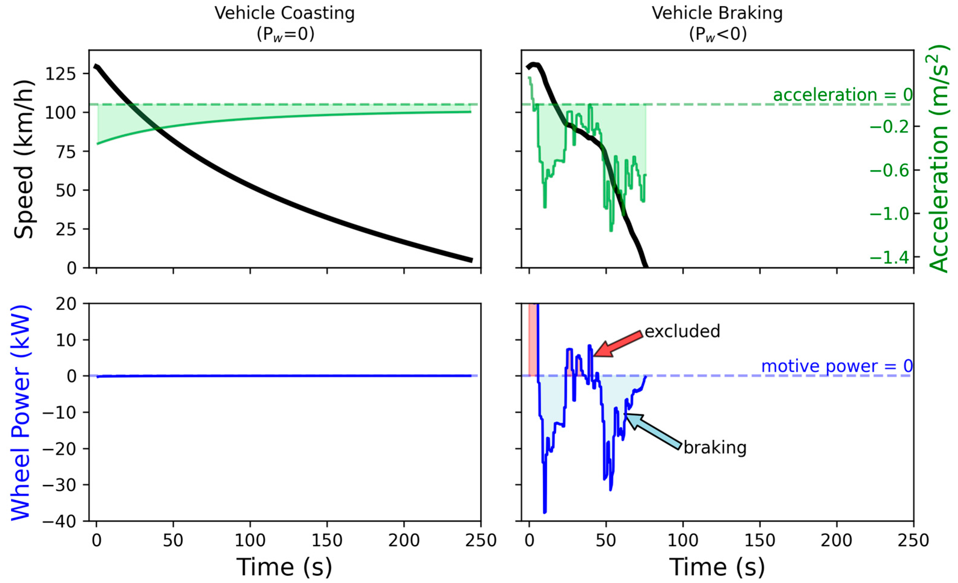
2.1.2. Coasting and Braking

It should be emphasized that the deceleration phases do not fully coincide with the braking phases. Figure 1 shows two examples of vehicle deceleration. Figure 1 (left panels) shows a vehicle coasting from a speed of 130 km/h. During coasting, a vehicle is left to decelerate with its wheels disengaged from the powertrain, i.e., the drivetrain, the ICE and the EMs. No friction braking is applied. In this case, the deceleration is produced only by the road loads, P w   =   0 (Equation (3)), and there is no friction braking applied. Such parts of decelerations should not be taken into account in the calculation of the c f r i c t i o n .
Figure 1 (right panels) plots a deceleration from 130 km/h as this is realised in the last deceleration phase of a worldwide harmonised light vehicles test procedure (WLTP) exhaust cycle. Compared to the coasting case of Figure 1 (left panel), the speed drop is steeper. The deceleration is supported by the friction braking applied by the driver, drivetrain friction, and energy recuperation through EΜs, depending on the powertrain configuration. There is one part in Figure 1 (right panel), which gives positive P w . This is a case where the deceleration is less than what would be achieved via the road load’s natural braking, thus, there is some positive power flowing to the wheels (propulsion). Indeed, at such instances, the driver needs to slightly press the accelerator pedal to keep the speed profile of the test cycle. The positive P w is excluded from the calculation of the deceleration energy (braking phase). Even though there is deceleration, taking that energy into account (when P w   >   0 ) would result in a higher c f r i c t i o n (see Equation (11)). Thus, in our analysis, braking events are defined based on the calculated power at the wheels and not the negative accelerations.

2.2. Experimental Setup

2.2.1. Vehicle

The vehicle was a plug-in hybrid with its main characteristics summarised in Table 1. The brake pressure signal was collected from the extended on-board diagnostics (OBD), and we considered that the pressure was the same for both front and rear axles ( p F A   =   p R A ). The validity of this assumption will be discussed later. Market fuel was used for all tests.

2.2.2. Chassis Dynamometer and Cycles

The tests were carried out on a chassis dynamometer compliant with UNECE Regulation 154 and GTR 15. The procedure for the determination of the friction braking share followed as closely as possible GTR 24 (Annex C), with any differences explained below. The same experienced driver drove the car in the laboratory tests. Two separate campaigns were performed with the same car (Table 2). The chassis dynamometer was set in road simulation all-wheel driving mode. For the all-wheel driving mode, the force distribution was assumed to be 77% (front axle) to 23% (rear axle). Note that typically, the sum of the front and rear force distribution is above 100% to take into account the inertia of rotating parts. However, in order to be closer to the procedure of Annex C of the GTR 24, where there is no distribution to front and rear axles for the calculation of the friction braking share coefficient, we applied values to give a sum of 100%. The actual speed was provided by the chassis dynamometer. The temperature of the test cell was 23 °C (the regulated temperature) or 31 °C (±2 °C) (outside the regulation boundaries). In most cases, the battery was fully charged, but for some tests, only partly (see Table 2). Note that GTR 24 requires a fully charged battery, but we applied a lower state of charge (SOC) in some tests to see if there was any impact on the results.
In the first campaign, the focus was on the different SOC and ambient temperature. The selected road load coefficients were F 0 = 174.4 N, F 1 = 0.7 N/(km/h), F 2 = 0.026 N/(km/h)2, accumulating 13,179 kJ of positive cycle energy demand in WLTP exhaust class 3b theoretical profile. In the second campaign, the focus was on the braking style. The official vehicle-specific road load coefficients were used, as derived following Regulation (EU) 2017/1151 [30] and reported to the vehicle’s certificate of conformity: F 0 = 121.2 N, F 1 = 0.93 N/(km/h), F 2 = 0.024 N/(km/h)2. This set of road load coefficients accumulates 12,266 kJ in WLTP class 3b. The second campaign used the official coefficients of the vehicle, while the first campaign simulated higher friction conditions. In the second campaign, the braking style was assessed by exploring deceleration ratios resulting in vehicle speeds outside or close to the regulation boundaries of the WLTP brake cycle. Thus, tests were performed with smooth, moderate, and aggressive braking styles apart from normal braking styles, respecting the regulation speed tolerances.
The WLTP exhaust cycle is used for pollutants and CO2 emissions and fuel efficiency benchmarking (Regulation 2017/1151 [30]) (Figure 2). However, this cycle was not designed to be representative of braking behaviour. For the determination of the brake emissions, the WLTP brake cycle is applied on a brake dynamometer (GTR 24). For the determination of the c f r i c t i o n on the chassis dynamometer, the whole WLTP brake cycle, or just the last part called Trip 10, can be used. For our tests, we used only Trip 10 and WLTP exhaust. In Figure 2, the speed profiles of the two certification protocols are shown, together with Trip 10.
Figure 3 shows an illustration of the different braking styles during Trip 10: normal (according to the regulation), and then the extreme cases: smooth, moderate, and aggressive (i.e., harder than the common ones defined by the regulation speed profile). Compared to the normal speed profile, it is evident that in the smooth braking, the braking starts earlier and finishes later (longer and smoother decelerations) resulting in lower acceleration spikes. In contrast, in the moderate and aggressive braking, the decelerations are more abrupt but still respect the regulation tolerances (grey shaded area). The difference between aggressive and moderate is that the latter does not fully take advantage of the speed tolerances, but there are more braking events during the deceleration. The moderate style simulates an inexperienced driver trying to follow the speed profile, pressing often and abruptly the brake pedal, while the fully aggressive simulates a driver taking advantage of the regulation tolerances.

2.2.3. Determination of Cp

For the determination of C p (i.e., the ratio of the brake torque and brake pressure), the chassis dynamometer was set at a constant speed of 30 and 50 km/h, and the driver was braking abruptly and shortly (Figure 4a). This is a specific dynamometer mode moving the vehicle, and not a road simulation as at the previous tests. Even when the driver tries to brake the vehicle, the dynamometer applies additional force to keep the speed constant. This way, the braking power can be calculated. The reason for not performing smooth braking events was to minimize energy recuperation. Furthermore, all tests started with a fully charged high-voltage battery. The ambient temperature and vehicle driving mode were set to the corresponding values of the main tests.
Due to the specific chassis dynamometer setting (constant speed fixed by the dynamometer), we could assume that the brake torque was equal to the one measured from the chassis dynamometer. The torque was calculated by multiplying the force measured by the chassis dynamometer with the dynamometer radius (Figure 4a). The brake pressure was given by the OBD. The C p was assumed to be the slope of torque and brake pressure (see Figure 4b). For all calculations, we applied fixed values, the average of all tests’ slopes: 37.0 Nm/kPa (±35%) for the front brakes and 13.5 Nm/kPa (±45%) for the rear brakes. If we didn’t fit the line through the origin (zero), the values would be approximately 35% higher and would result in 35% higher friction braking share coefficients (Equations (6), (10) and (11)). We took the average value, as data points with low pressure and high brake torque might be impacted more by the regenerative capabilities of the vehicle, and consequently overestimate the capabilities of the friction brakes.
The estimation of the C p from the chassis dynamometer does not necessarily represent the average value over the laboratory cycles or even the actual value on the road. For example, (brake) temperature can have an impact on the C p value [31]. Considering the uncertainty of the estimated value and the impact of actual conditions, the value we used should be considered as an approximation. The regulated procedure requires estimation of the C p value applying the WLTP brake cycle.
In real life applications, the pressure distribution between axles differs to improve stability and control during braking. This variability and the pressure reduction at the rear brakes was partly covered during the determination of the C p . However, not all cases can be captured with the few braking events at the dynamometer. Thus, it is possible that during the laboratory or on-road tests the pressure at the rear brakes would be lower, and the friction braking share coefficient lower.

2.2.4. Real-World Trips

To address the contribution of the friction braking under real-world conditions, we selected some trips from a real-world campaign performed by the Joint Research Centre (JRC) in 2024 with a total distance of 10,900 km [32]. The trips took place in northern Italy mostly, with 10 different drivers. Details of data acquisition and trips analysis can be found in previous campaigns [33,34]. In short, among other parameters, the vehicle speed and the brakes pressure were recorded from the OBD. We considered urban trips as those with a total distance between 2 and 20 km, and urban driving share higher than 50%. The urban, rural, and motorway time share were calculated for each trip following the principles of the Regulation (EU) 2017/1151 [30]: speeds below 60 km/h were considered as urban driving, speeds between 60 and 90 km/h as rural driving, and speeds above 90 km/h as motorway driving. Since many trips met this condition (502 trips), one trip was selected per 1 km interval from inside the range of 2–20 km; that is the one having the closest average speed to the sample of that interval. As a result, 18 trips with urban characteristics were derived. We considered rural trips those with distances above 5 km, and rural share above 50%; in total, 11 rural trips were found. We considered motorway trips, those with distances above 100 km having 50% or more of highway share; in total, 20 trips. Additionally, we selected 7 trips resembling the characteristics of the trips prescribed in the real-driving emissions (RDE) regulation (2017/1151) [30]. The RDE-proxy trips had distances between 30–100 km, and balanced urban, rural, and highway shares between 20 and 50%. In total, we analysed 56 trips, covering a distance of 5000 km. Additionally, the full dataset containing 786 trips was also assessed in the same way in order to provide a lifetime value for the friction brakes share calculated for the 10,900 km driven between March to December of 2024.
The trip average ambient temperature recorded during the trips spanned from 4 °C to 36 °C (1st and 99th percentile, respectively) for both reduced dataset of 56 trips and the full dataset. Information about the precipitation and snow was not recorded during the trips, but they were later retrieved via an Application Programming Interface (API) from Meteostat Python Package [35], version 1.7.4, for the GPS coordinates in the middle distance of each trip. According to this information, the average precipitation was 4%, with 14% and 56% for the 90th and the 99th percentiles, respectively, overall, denoting limited rain during the trips. Regarding snow, the API showed snow only for one day and 4 trips, which are not included in the reduced dataset of 56 trips.
Regarding the topography of the area, the 56 selected trips are placed inside a radius of 60 km around Milan, covering cities such as Varese, Bergamo, and Piacenza, with the vast majority of trips held near Varese, where the JRC is located. RDE-proxy and motorway trips showed the highest variations in elevation between start and finish, with absolute elevation difference averaging 195 m, but also reaching 500 m (90th percentile) or above in the case of RDE-proxy. Rural trips elevation change was limited, averaging 18 m, with a 90th percentile of 30 m. The 18 urban trips had a change in the elevation averaging 58 m, with a 90th percentile of 140 m. Regarding the total number of trips meeting the criteria set for urban driving, the average absolute difference in elevation was 58 m, with a 90th percentile value of 53 m.
Combining Equations (2) and (3), the power at the wheels is calculated via the kinematics equation calculated using the road load coefficients, the vehicle mass, and the actual speed profile. In the laboratory, the calculated wheel power has high accuracy as the dynamometer is adjusted with the road load coefficients and the test mass. However, this is not the case for on-road conditions. Environmental and traffic parameters such as road surface quality, ambient temperature, humidity, and car following schemas can affect the road load coefficients. These variations result in discrepancies between the calculated wheel power via the (fixed) road loads and the actual power realised under real-world conditions [29]. Additionally, during the real-world campaign, the passenger occupancy or extra load was not recorded to have a better understanding of the actual vehicle mass. For simplicity, the official road load coefficients and test mass were also used for the real-world assessment, since these are designed to be realistic in-use conditions. For example, the test mass value that was used according to the certification regulation includes some extra load for real-world representativeness. For the calculation of the braking energy at the wheels in the real world, the slope of the road was also considered.
The area is rather mountainous, as it is visible via metrics presented for the altitudes covered during the trips, and might not fully reflect the typical terrain, as for example, a typical urban area of a city in Europe. In general, although the environmental and traffic conditions (and others such as vehicle load, road surface, and topography) have an impact on the use of friction brakes, the driving style (including the braking energy) has an even higher impact, as it will be shown later.

3. Results

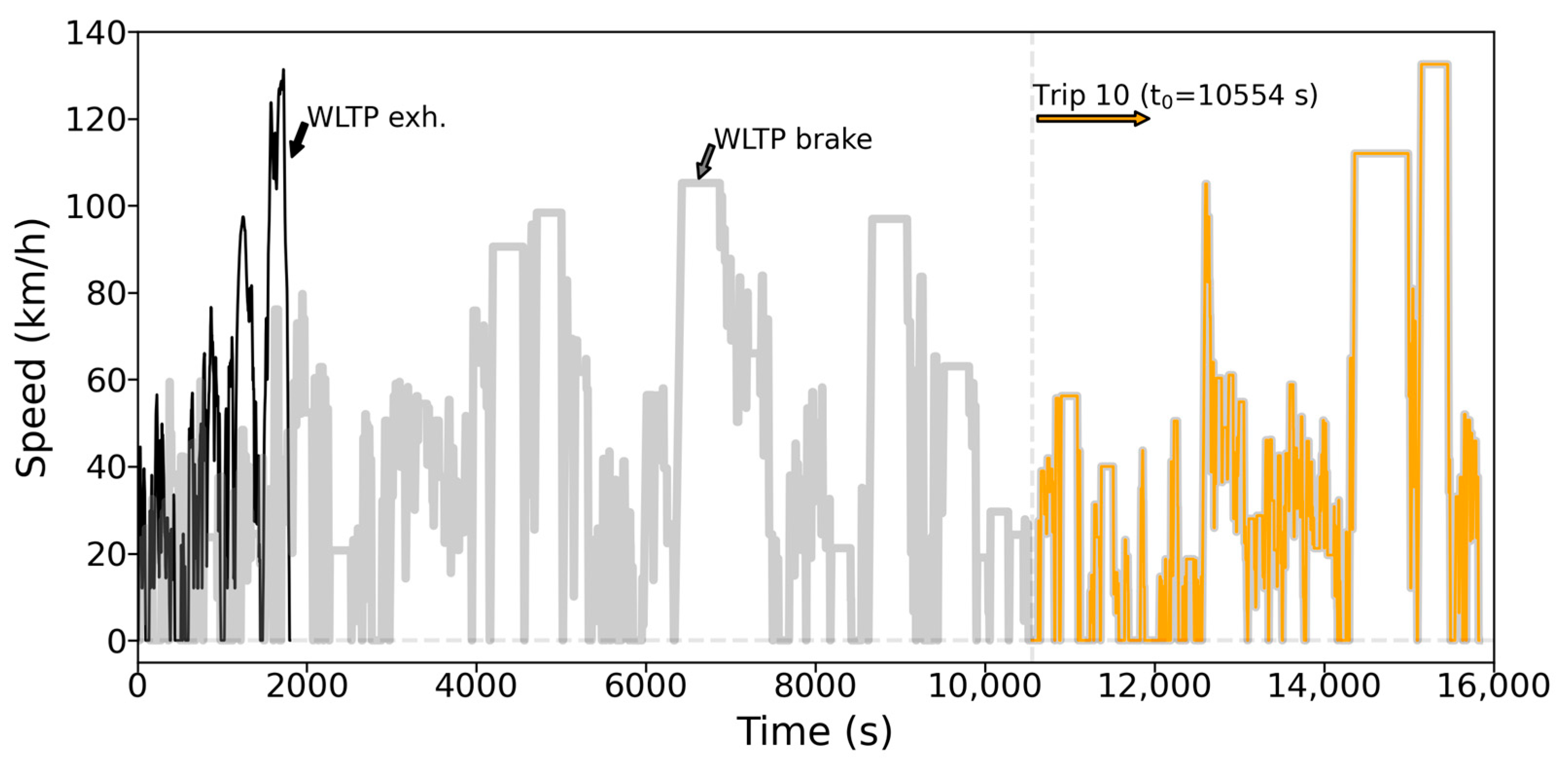
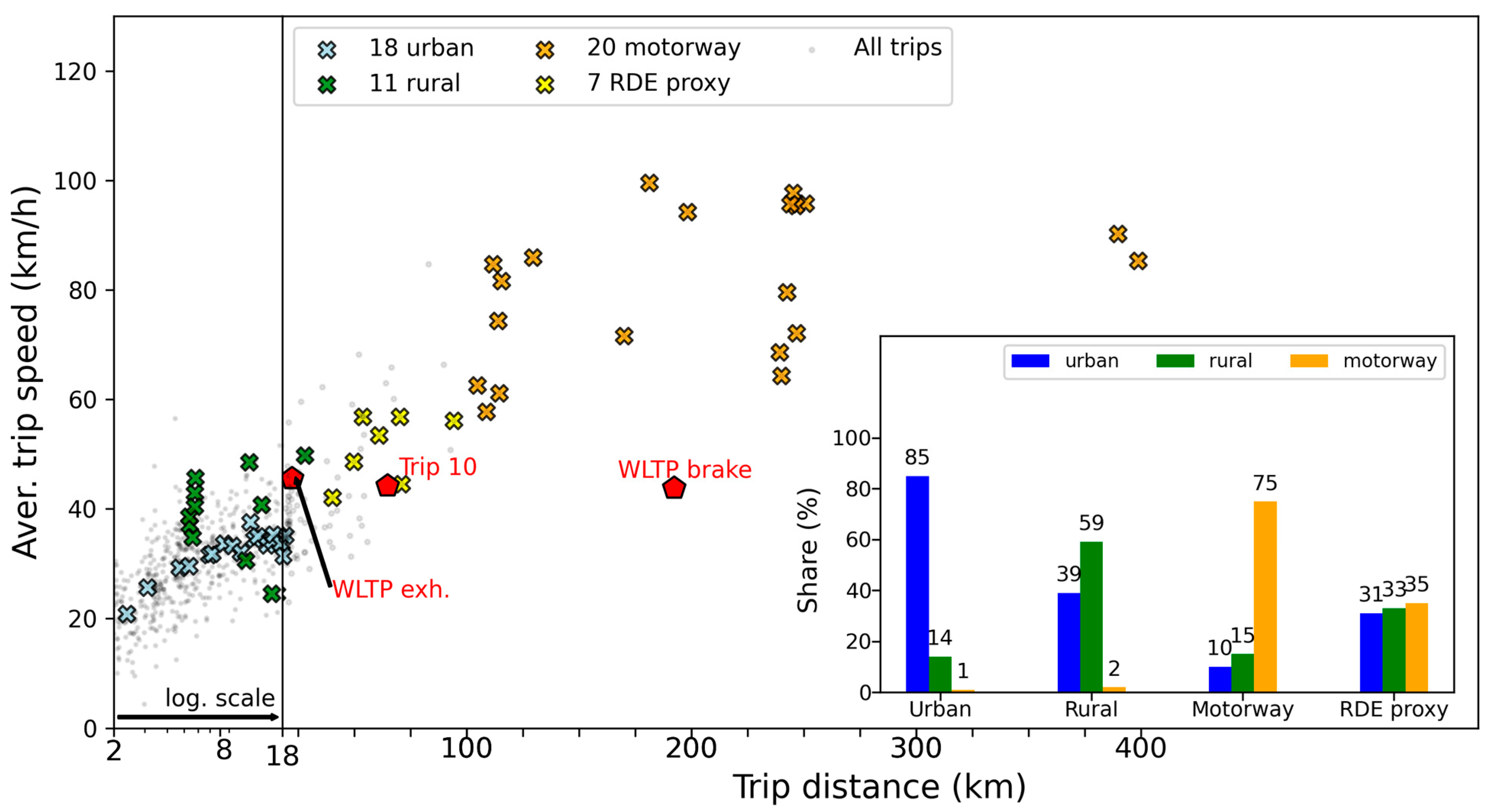
3.1. Characteristics of Real-World Trips

Figure 5 provides an overview of the urban, rural, motorway, and RDE-proxy trips. The figure plots average speed and distance, while the distance-weighted share of urban, rural, or motorway driving is given in the inset. Based on our definitions (see experimental part), the urban trips were on average 11 km long, with an average trip speed of 32 km/h. The driving was mainly below 60 km/h, overall accumulating 85% of urban driving. Rural trips’ average distance was 10 km, with an average trip speed of 40 km/h, having a mainly rural share of driving of 59%. The 20 motorway trips selected had an average trip distance of 205 km, and an average trip speed of 81 km/h. The motorway trips consisted of 75% of motorway driving, 10% of urban, and 15% of rural driving. Finally, the 7 RDE-proxy trips had an average trip distance of 63 km, with an average speed of 51 km/h, and urban/rural/motorway driving balanced around 33%.

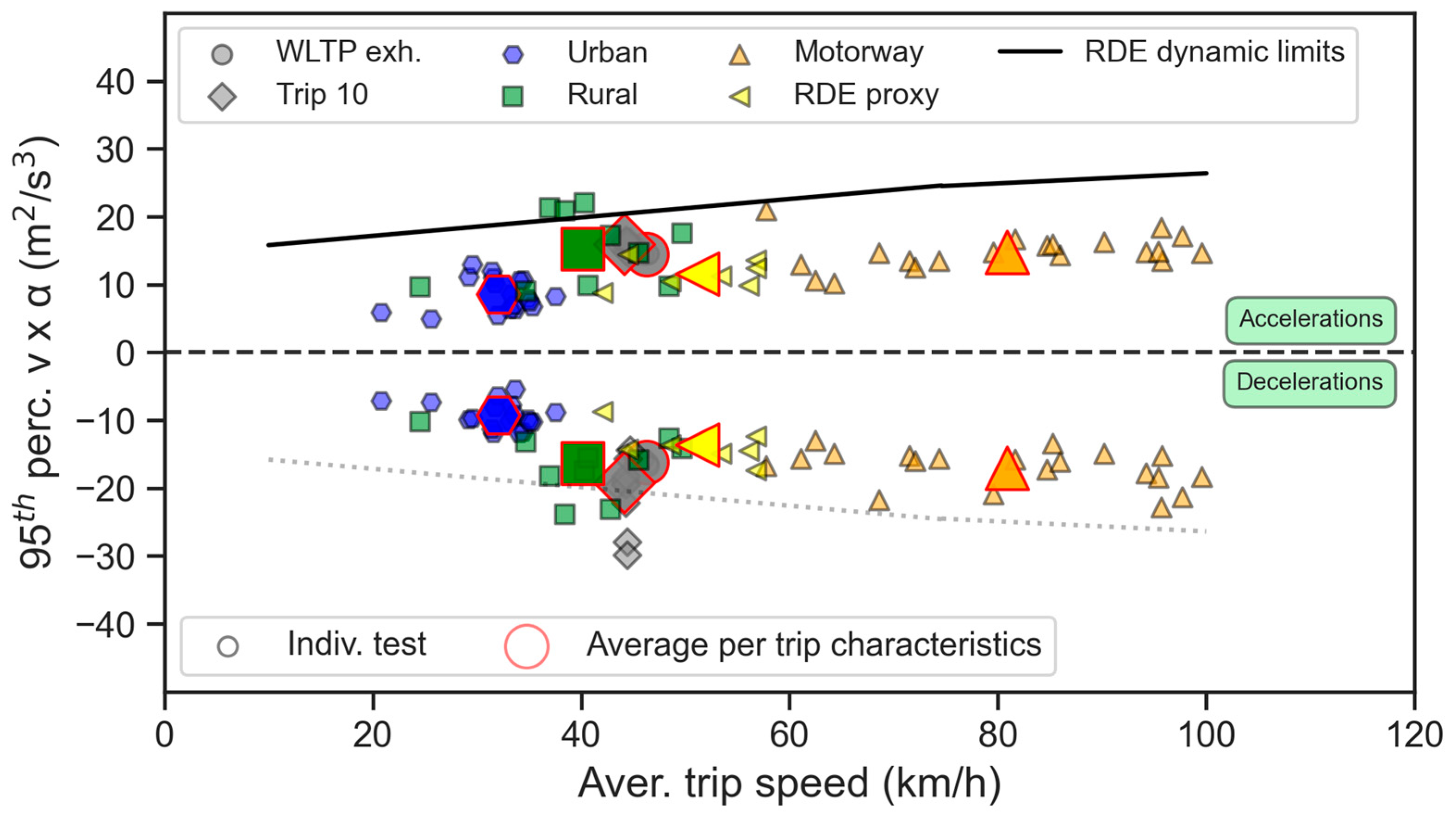
3.2. Dynamics of Laboratory Cycles and Real World Trips

In this sub-section we provide some quantitative characteristics of the cycles followed in the laboratory and on the road. Figure 6 plots the 95th percentile of the positive accelerations times the average speed ( v   ×   a ), an index typically used in RDE regulation to check the driving dynamics. Although the focus of the paper is the braking (decelerations), for informative reasons, we provide the values for the acceleration events to give indications of the tested cycles compared to other cycles in the literature. As described in the Regulation (EU) 2017/1151 [30], the acceleration phases were restricted to the ones having accelerations above 0.1 m/s2 for positive accelerations. We also applied the same criterion for the decelerations (i.e., lower than −0.1 m/s2 for the decelerations). An indicator for the dynamicity of the real-world trips is the proximity of the 95th percentile v   ×   a against the RDE limits, as they are defined in Regulation (EU) 2017/1151 [30]. The v   ×   a limits are 18.5 m2/s3 at 30 km/h average speed, 20.6 m2/s3 for 45 km/h, 24.5 m2/s3 for 75 km/h, and 26.4 m2/s3 for 100 km/h.
The 95th percentile of v   ×   a for WLTP exhaust cycle and Trip 10 were quite close (Figure 6 upper part). The on-road rural trips were on average close but show a high spread, with some trips exceeding the regulation boundaries. The on-road urban trips had lower v   ×   a values, while the RDE-proxy trips showed a low range of v   ×   a values and they were on average between urban and motorway trips.
In Figure 6 (lower part), the distributions of the 95th percentile of the deceleration times the average speed are presented for different trips. On average, the WLTP exhaust cycle had similar decelerations to real-world rural trips. The urban trips had the lowest (absolute) values, while the RDE-proxy trips were between urban and motorway. Trip 10 had the highest (absolute) values, with the aggressive braking styles reaching very high values.

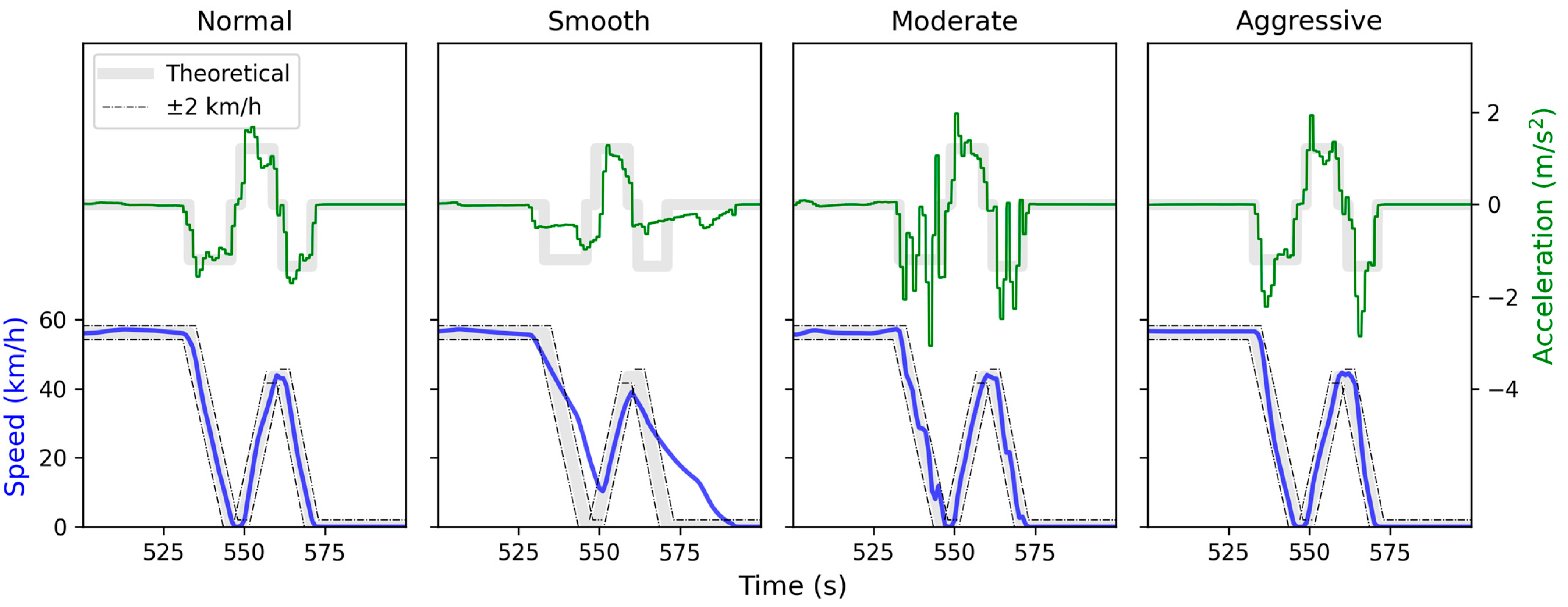
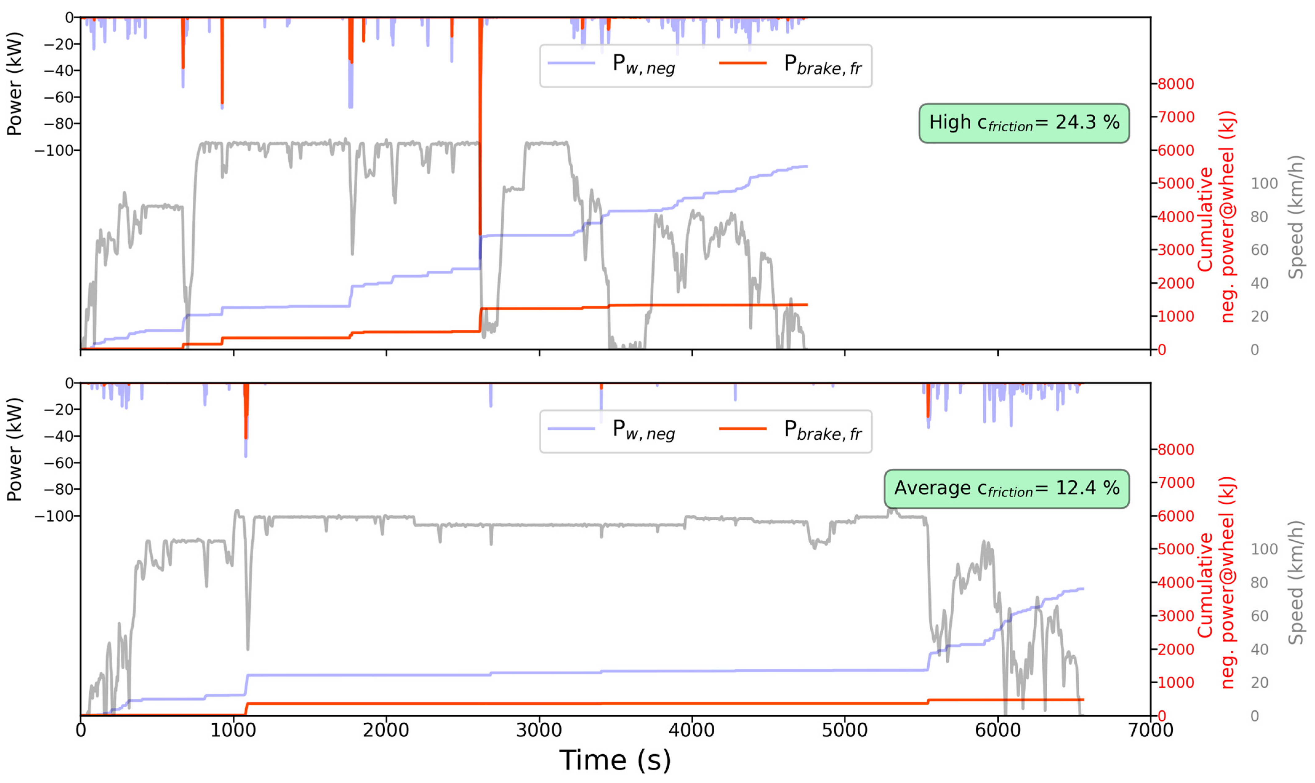
3.3. Real-Time Examples of Braking

Following the GTR 24 procedure for the identification of the braking events, the WLTP brake cycle has 303 braking events identified from the theoretical speed profile, while Trip 10 has 114 events. Applying the same procedure for the WLTP exhaust theoretical speed profile, 54 events were identified. Figure 7 presents some representative real-time experimental results from the laboratory tests. For each individual test, the calculated P b r a k e , f r (in red) is overlapped with the negative power at wheel, P w , n e g (in blue). The average P b r a k e , f r for WLTP exhaust is −0.35 kW, with peaks reaching −3.4 kW (the red lines are hardly visible in the graph). For the normal Trip 10 test, the mean friction brake power was −1.9 kW, reaching up to −36 kW. Friction brakes were used at 46 out of the 114 events. In the aggressive Trip 10, the average power on the brakes was −6 kW, and reached −135 kW.
The overall distributions of the friction brakes share per brake event are presented in Figure 8. The shares of 0%, i.e., friction brakes not activated during braking, have been excluded. In the normal Trip 10, the average energy share attributed to friction brakes inside the remaining 46 events with share greater than 0%, was 19.7%. For the Trip 10 performed with smooth decelerations, the friction brakes were used in 36 events, having an average friction share of 26.7%. The reason the average brake share is higher in the smooth braking style compared to the normal is that there is a lower number of events with braking share higher than 0%, and secondly, the actual braking phases were sometimes falling outside the strict phases considered in the GTR 24, as also seen in the examples in Figure 3. For Trip 10, performed with more aggressive braking, the friction brakes were used at 110 events out of the total 114. The average energy share of friction brakes was 28%. Finally, for the WLTP exhaust, friction brakes were applied at 8 out of the 54 events, having an average energy share of 8% for the friction brakes.

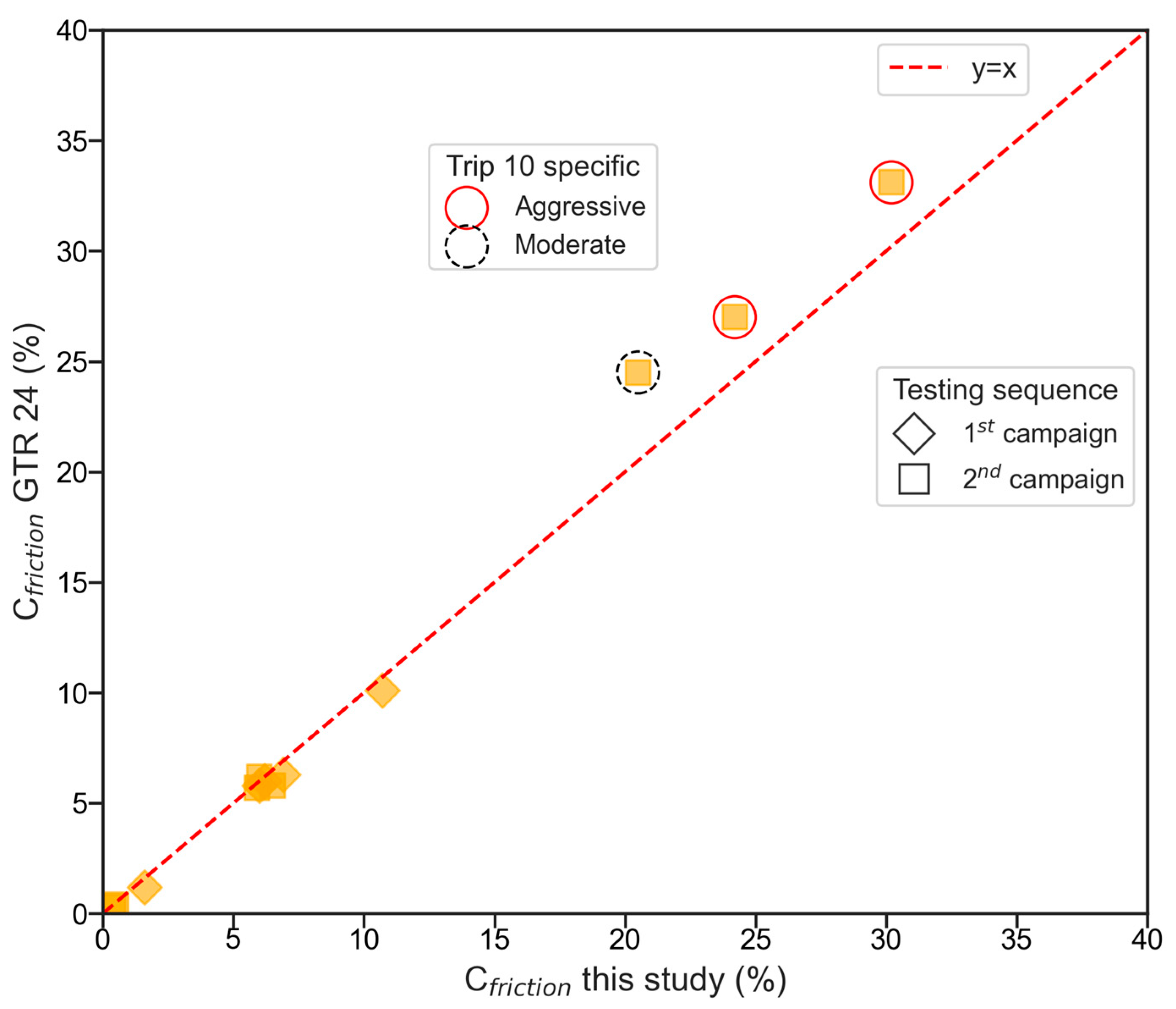
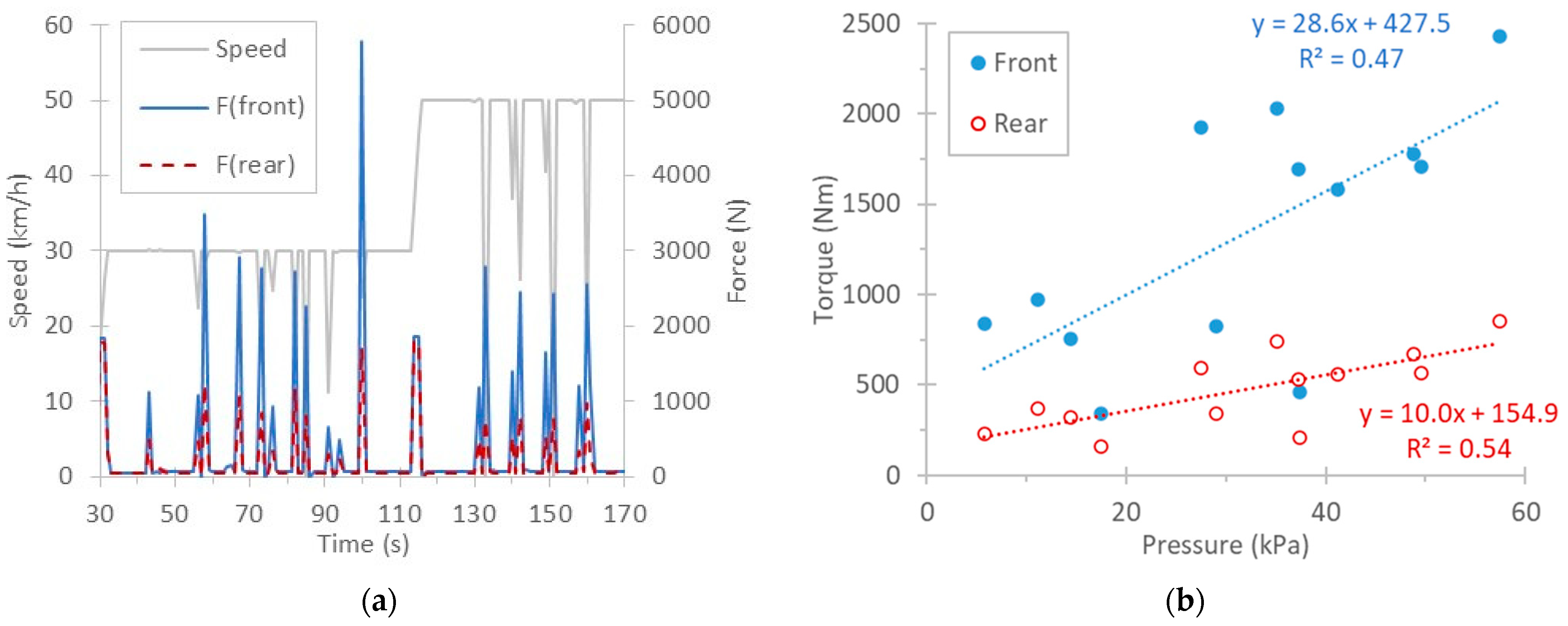
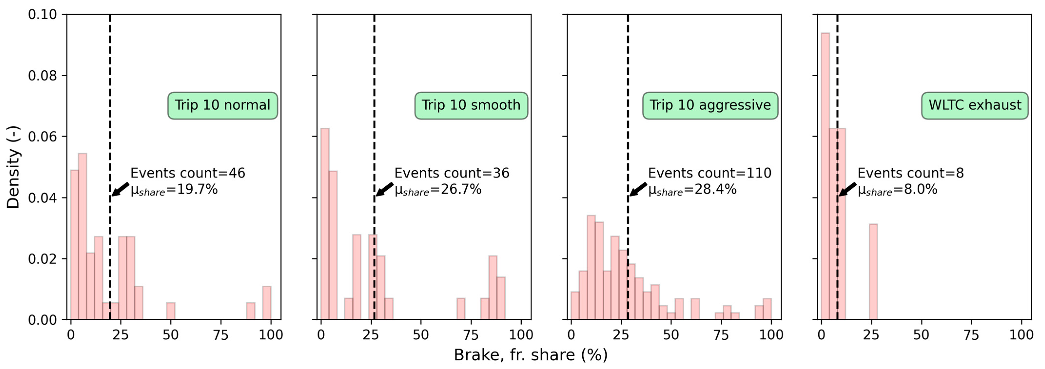
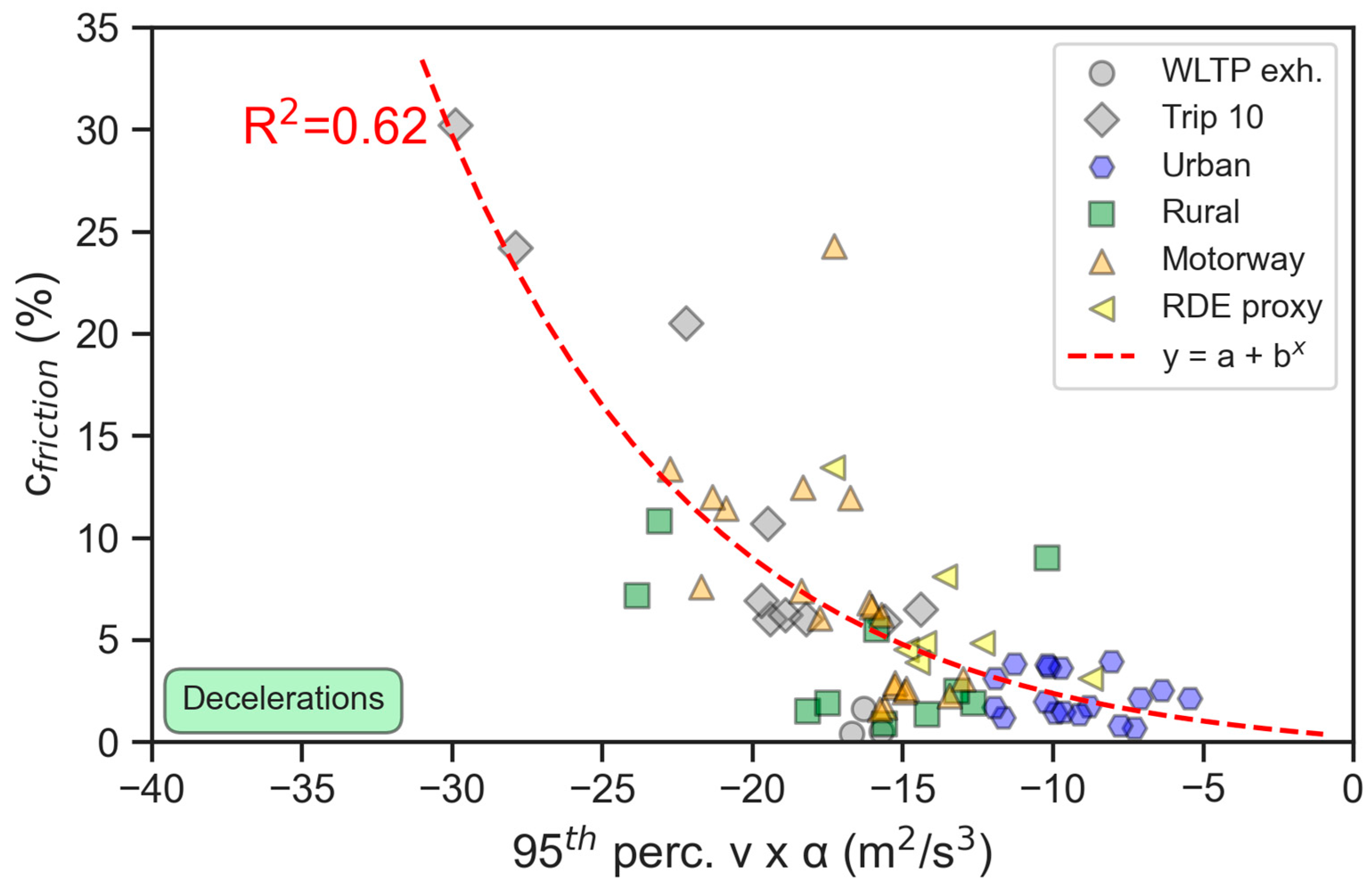
3.4. Friction Braking Shares

Figure 9 summarises the friction braking share coefficients for the laboratory and on-road tests. For the tested plug-in hybrid vehicle at the WLTP exhaust test, the average friction braking share coefficient c f r i c t i o n was 0.8% with a maximum of 1.6%. The five normal Trip 10 had c f r i c t i o n on average 7.2%. For the two tests performed with smooth decelerations, an average coefficient of 6.2% was calculated. The coefficient for the moderate Trip 10 was 20.5%, while the two aggressive tests had coefficients of 24.2% and 30.2%. The 18 selected urban trips showed lower friction share coefficients ranging from 0.7% to 3.9%. As explained in the description of the topography of the area that the real-world campaign took place, some of the selected urban trips have a high altitude difference between start and finish, possibly not fully representing a typical urban area. To confirm the validity of the results for the urban conditions, the range of c f r i c t i o n values from all the 502 trips meeting the criteria of urban driving is presented in Figure 9. The comparison of the distributions of the two samples for the urban conditions shows the validity of the initial results. For rural driving, there was a high spread of values, with the majority ranging below 3%, but there were also values reaching 10.8%, altogether averaging to 4.2%. For the trips performed in motorway conditions, three separate clusters were observed, one with values below 4%, one with values ranging between 6 and 8%, and one between 11 and 14%. There is a trip with coefficient of 24.3%. The difference between these clusters is the existence of sudden braking events with a big part of the energy dissipated via the friction brakes, as it will be discussed in the next paragraphs. Altogether, the c f r i c t i o n in motorway driving averaged at 7.3%. Finally, the trips selected as proxy of RDE showed an average c f r i c t i o n of 6.1%.
The c f r i c t i o n values derived from the full real-world dataset consisting of 786 trips are also presented in Figure 9. Accordingly, an understanding of the lifetime friction brake usage can be derived. The median value of c f r i c t i o n was 2.4% and the of 25th–75th percentiles were 1.4% and 4.4%, respectively. Accounting for the distance of each individual trip, the lifetime distance-weighted c f r i c t i o n was calculated to 5.3%. It should be recalled that these trips were performed around rural areas in Northern Italy.
It should be emphasised that the data of this study apply to one specific plug-in hybrid and findings cannot be generalised to other plug-in hybrids, mild/full hybrids or battery electric vehicles. For example, a study from the International Organization of Motor Vehicle Manufacturers (OICA, in French Organisation Internationale des Constructeurs d’Automobiles) presented c-factors ranging from 5% to 18% for plug-in hybrids [36].
As explained in the methodology section, the official test mass and road load coefficients were used for the determination of the power at the wheels under real-world driving. Since data were not available for considering the dependence of the actual mass during the campaign, a sensitivity analysis on the c f r i c t i o n was performed by fluctuating the mass by ±10%, i.e., 175.3 kg. Accordingly, the F 0 coefficient, which is dependent on the normal force applied by the vehicle’s weight [29], was normalised to the new mass of the vehicle. Table 3 presents the mean values using the official test mass and the road load coefficients, and the two extreme scenarios with a ±10% change in the test mass. The change in the mass had limited impact on urban and rural driving, which was below 0.6% absolute. The highest change appeared in motorway and RDE-proxy conditions, where the change of the mass influenced the c f r i c t i o n by up to 1% absolute. Overall, it can be safely assumed that the use of the official test mass and road load coefficients fits the purpose of the analysis, and has minimal impact on the results (<1% absolute or <15% relative).
To better understand the high scatter of braking shares under real-world conditions, Figure 10 shows two different examples of motorway trips with c f r i c t i o n of 24.3% and 12.4%. The top figure shows a motorway trip with abrupt decelerations from high speeds. In this case, the negative power at the wheels is high, reaching values above 150 kW. This is because of the high speed and the respective kinetic energy of the vehicle that the driver tries to reduce. The vehicle at these moments likely uses friction brakes to a larger extent due to safety reasons [37,38]. Additionally, as specified in Table 1 with the vehicle characteristics, the maximum motor power is 120 kW. Thus, in such high deceleration powers developed at the wheels, the electric motor of the vehicle cannot absorb such an amount of power. In contrast, the bottom figure of Figure 10 shows a motorway trip with less use of friction brakes. Still, there are times when friction brakes consume high shares of the kinetic energy due to steep decelerations. Anyhow, such decelerations are less frequent, resulting in lower c f r i c t i o n values compared to the trip in the upper panel. The figures confirm that the high values of c f r i c t i o n at the motorway trips of Figure 9 are not outliers but real braking behaviour.
Figure 11 plots the c f r i c t i o n values as a function of the 95th percentiles of the v   ×   a . The exponential fitting of the results (R2 = 0.62) and indicates an acceptable correlation of the two parameters, although the variability is not entirely captured. In other words, a higher contribution of friction brakes is expected with more aggressive braking. Similar trends can be seen plotting c f r i c t i o n in function of the quality criteria in GTR 24: the Inertial Power Difference Rating (IPDR (%) and Work IPDW (J/kg). However, they are not plotted as these parameters are available only for laboratory tests.

4. Conclusions

In this study, we first developed a methodology to calculate the contribution of friction brakes to vehicle decelerations (braking). The methodology is based on the regulated procedure for laboratory tests. We expanded this approach to driving cycles where the speed profile is not prescribed, such as during on-road trips. We defined the friction braking share as the ratio of the friction power calculated from brake discs pressure to the total negative power at the wheel during the braking event.
Our approach gave almost identical results with the regulated method for the regulated test cycles. Some differences were noticed, as expected, when the driver was intentionally deviating from the prescribed cycle. Nevertheless, the methodology has also some limitations. The negative power at the wheels strongly depends on the vehicle road load coefficients (friction and coasting), which is a critical factor for the c f r i c t i o n estimation. In real-world applications, road load coefficients are unknown and this causes uncertainty. Laboratory tests with different F 0 values did not reveal any significant impact on the friction share coefficient. Similarly, variation of the ambient temperature between 23 and 32 °C or the SOC of the battery did not impact the c f r i c t i o n . Variations of the mass (±10%) had an almost proportional impact (12–15%). Our calculations used a fixed value for the C p (coefficient that captures the friction properties of the brakes), based on a few laboratory braking events. Thus, the absolute value we used has some uncertainty. Furthermore, the value can change during driving, depending on the actual brake temperature e.g., due to the braking frequency or travelling speed that impacts the brakes cooling. We also used the brake pressure we had available at the vehicle’s OBD. However, the actual pressure at the brakes might be different and even variable depending on the driving conditions. Future studies need more detailed modelling to quantify the impact of these parameters. In general, our results showed that their impact is rather small (<2% absolute in the friction coefficient) compared to the braking style (smooth or hard) (impact 5–25% absolute).
In a second step, we analysed the contribution of friction brakes during braking events in laboratory and on-road tests for a plug-in hybrid vehicle. The laboratory cycles included certification tests for exhaust (WLTP exhaust) or brake emissions (Trip 10 from the WLTP brake cycle). Braking style ranged from smooth to aggressive (harsh). The on-road tests, covering a distance of over 10,900 km with 10 different drivers, were categorised into urban, rural, motorway, or real-driving emissions (RDE) proxy trips. The average friction braking share was around 7% for the laboratory Trip 10, while 5% was found for the selected real-world trips. In more detail, urban and rural trips showed low median c f r i c t i o n values of 2.1%, but the average c f r i c t i o n for rural was 4.2% due to some trips with high values. Motorway and RDE proxy trips showed higher values, averaging to 7.3% (median 6.4%) and 6.1% (median 4.8%), respectively. A few motorway trips reached values of 12–25%, while laboratory Trip 10 tests with deliberately aggressive braking reached values of 22–32%. The lifetime distance-weighted value for the whole real-world campaign showed a c f r i c t i o n value of 5.3%. Overall, the friction braking share was found to moderately correlate exponentially with the 95th percentile of speed multiplied by deceleration, a metric derived from exhaust regulations to characterise trip dynamics from accelerations.
The results confirm the suitability and representativeness of the brake laboratory cycle. Additionally, we demonstrated the variability of the friction brakes’ contribution under real life conditions, providing some first values to support literature in the field. Our methodology could be applied in future testing of the friction braking share coefficients on the road for research or market surveillance purposes, as at the moment, only in-service compliance testing in the laboratory is foreseen.

Author Contributions

Conceptualization, B.G. and T.G.; formal analysis, D.K.; writing—original draft preparation, D.K. and B.G.; writing—review and editing, A.T., G.T. and G.F. All authors have read and agreed to the published version of the manuscript.

Funding

This research received no external funding.

Data Availability Statement

Dataset available on request from the authors.

Acknowledgments

The authors would like to acknowledge the technical staff of VELA 8 (M. Centurelli, M. Stefanini, A. Bonamin, and E. Longo) for running the tests. The authors acknowledge JRC BDAP (Big Data Analytics Platform) for hosting the data for this study.

Conflicts of Interest

The authors declare no conflicts of interest. The information and views set out are those of the authors and do not necessarily reflect the official opinion of the European Commission. Neither the European Union institutions and bodies nor any person acting on their behalf may be held responsible for the use which may be made of the information contained therein. Mention of trade or commercial products does not constitute endorsement or recommendation by the authors or the European Commission.

Abbreviations

The following abbreviations are used in this manuscript:
APIApplication programming interface
EMElectric motor
EUEuropean Union
FAFront axle
FDForce distribution
ICEInternal combustion engine
IPDRInertial power difference rating
IPDWInertial power difference work
JRCJoint Research Centre
GTRGlobal technical regulation
NAONon-asbestos organic
OBDOn-board diagnostics
OICAInternational Organization of Motor Vehicle Manufacturers (Organisation Internationale des Constructeurs d’Automobiles)
PMParticulate matter
RARear axle
RDEReal-driving emission
SOCState of charge
UNECEUnited Nations Economic Commission for Europe
WLTPWorldwide harmonised light vehicles test procedure

Appendix A

Appendix A.1. Comparison to the Regulatory Method

In GTR 24 (Annex C), the friction braking coefficient c f r i c t i o n is calculated comparing the measured negative energy at the deceleration events (e.g., based on brake pressure measurements) to the theoretical negative energy of the deceleration event and applying a factor of 0.87 to take into account 13% of vehicle losses (Equation (A1)). There are two main differences compared to our approach, described in Section 2 of the main text: (i) the fixed 13% for vehicle losses; (ii) the fixed time periods and speed profile for the calculation of the measured and theoretical energy. Even though this approach makes sense in laboratory conditions and known cycles, it cannot be applied on real world trips, where there is no prescribed (theoretical) speed profile. Our approach in determining the energy when the power at the wheels becomes negative overcomes this issue.
Figure A1 compares the two methods for the laboratory Trip 10 cycles. The agreement is excellent for the normal trips, but we see deviations in smooth and aggressive driving. The reason is that the time periods of these extreme events are different from those prescribed in the regulation (braking in advance for smooth driving or last second for aggressive braking). Such examples were given in Figure 2 of the main text. Thus, our method is not only applicable for on-road tests, but also gives more accurate results for non-ideal driving style (which should not be the case for regulatory tests).
c f r i c t i o n , G T R 24 = E b r a k e , f r   a t   n e g . t h e o r   a c c e l   E t h e o r   k i n e t i c   a t   n e g . t h e o r .     a c c e l   · 0.87
Figure A1. Cfriction as calculated in this study versus as defined in regulation GTR 24, Annex C.
Energies 18 04104 g0a1

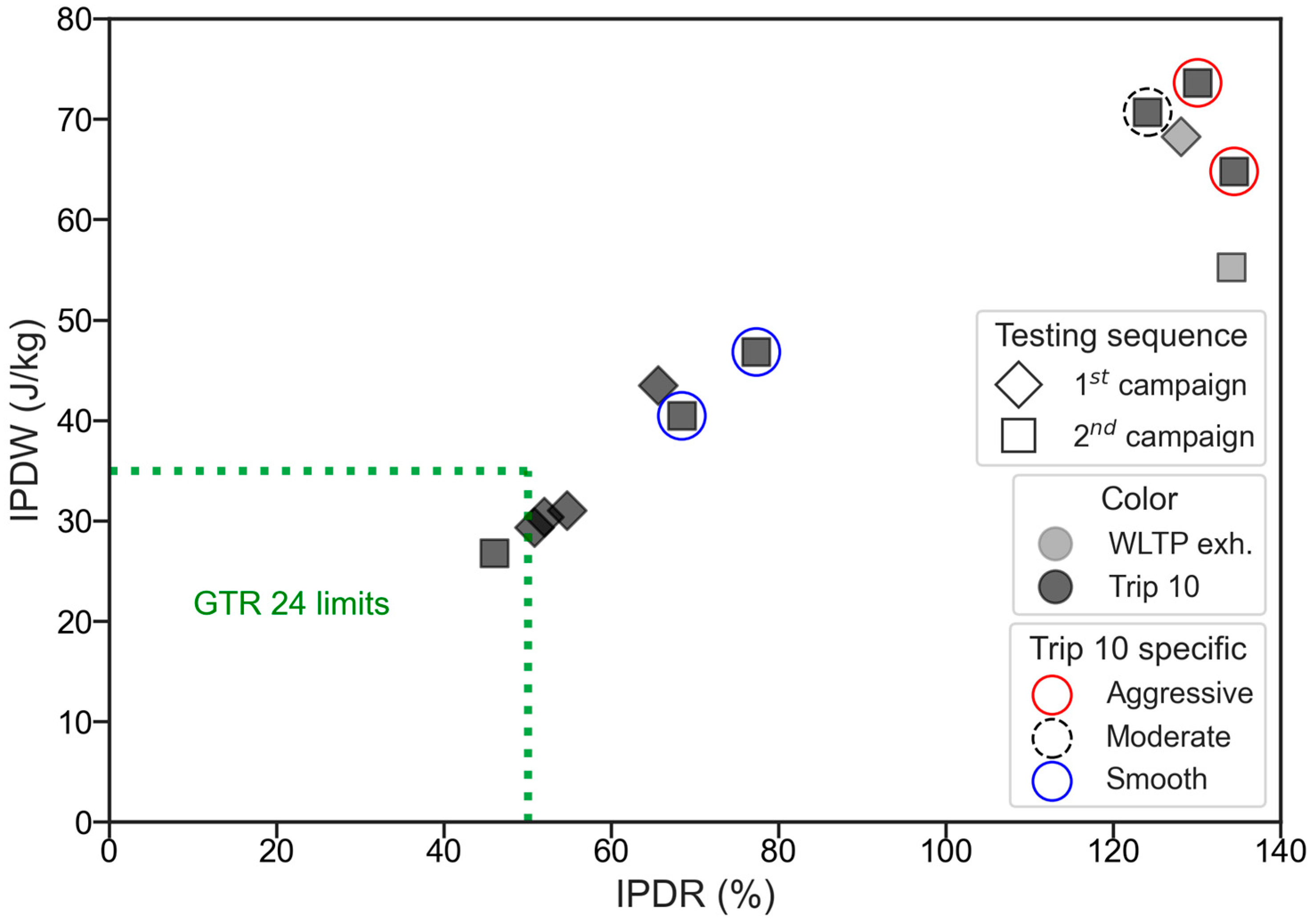
Appendix A.2. Test Quality Criteria for Laboratory Cycles

In order to assess the braking style of the driver, there are few quality criteria in GTR 24, the so-called inertial power difference rating IPDR (%) and work IPDW (J/kg). Figure A2 plots the values for the tests carried out and the limit values of the regulation. The normal trips are close to the limits, while smooth and aggressive are far outside, as expected. It should be emphasized that the criteria were developed for the complete WLTP brake cycle. For this reason, the WLTP exhaust cycle seems to be far away from the limit values. For Trip 10, the limits seem reasonable and would detect biased driving.
Figure A2. Laboratory tests driving quality criteria.
Energies 18 04104 g0a2

References

  1. Sicard, P.; Agathokleous, E.; De Marco, A.; Paoletti, E.; Calatayud, V. Urban population exposure to air pollution in Europe over the last decades. Environ. Sci. Eur. 2021, 33, 28. [Google Scholar] [CrossRef]
  2. Beloconi, A.; Vounatsou, P. Substantial Reduction in Particulate Matter Air Pollution across Europe during 2006–2019: A Spatiotemporal Modeling Analysis. Environ. Sci. Technol. 2021, 55, 15505–15518. [Google Scholar] [CrossRef]
  3. Wallington, T.J.; Anderson, J.E.; Dolan, R.H.; Winkler, S.L. Vehicle Emissions and Urban Air Quality: 60 Years of Progress. Atmosphere 2022, 13, 650. [Google Scholar] [CrossRef]
  4. Ravi, S.S.; Osipov, S.; Turner, J.W.G. Impact of Modern Vehicular Technologies and Emission Regulations on Improving Global Air Quality. Atmosphere 2023, 14, 1164. [Google Scholar] [CrossRef]
  5. Giechaskiel, B.; Grigoratos, T.; Dilara, P.; Karageorgiou, T.; Ntziachristos, L.; Samaras, Z. Light-Duty Vehicle Brake Emission Factors. Atmosphere 2024, 15, 97. [Google Scholar] [CrossRef]
  6. Hooftman, N.; Oliveira, L.; Messagie, M.; Coosemans, T.; Van Mierlo, J. Environmental Analysis of Petrol, Diesel and Electric Passenger Cars in a Belgian Urban Setting. Energies 2016, 9, 84. [Google Scholar] [CrossRef]
  7. Christou, A.; Giechaskiel, B.; Olofsson, U.; Grigoratos, T. Review of Health Effects of Automotive Brake and Tyre Wear Particles. Toxics 2025, 13, 301. [Google Scholar] [CrossRef]
  8. European Commission Regulation (EU) 2024/1257 of the European Parliament and of the Council on type-approval of motor vehicles and engines and of systems, components and separate technical units intended for such vehicles, with respect to their emissions and battery durability (Euro 7), amending Regulation (EU) 2018/858 of the European Parliament and of the Council and repealing Regulations (EC) no 715/2007 and (EC) no 595/2009 of the European Parliament and of the Council, Commission Regulation (EU) no 582/2011, Commission Regulation (EU) 2017/1151, Commission Regulation (EU) 2017/2400 and Commission implementing Regulation (EU) 2022/1362. Off. J. Eur. Comm. 2024, L, 1–49.
  9. Grigoratos, T.; Mamakos, A.; Vedula, R.; Arndt, M.; Lugovyy, D.; Hafenmayer, C.; Moisio, M.; Agudelo, C.; Giechaskiel, B. Characterization of Laboratory Particulate Matter (PM) Mass Setups for Brake Emission Measurements. Atmosphere 2023, 14, 516. [Google Scholar] [CrossRef]
  10. UNECE. UNECE Global Technical Regulation (GTR) 24; UNECE: Geneva, Switzerland, 2025; Available online: https://unece.org/transport/standards/transport/vehicle-regulations-wp29/global-technical-regulations-gtrs (accessed on 5 July 2025).
  11. Xu, G.; Li, W.; Xu, K.; Song, Z. An Intelligent Regenerative Braking Strategy for Electric Vehicles. Energies 2011, 4, 1461–1477. [Google Scholar] [CrossRef]
  12. Qiu, C.; Wang, G. New evaluation methodology of regenerative braking contribution to energy efficiency improvement of electric vehicles. Energy Convers. Manag. 2016, 119, 389–398. [Google Scholar] [CrossRef]
  13. Valladolid, J.; Calle, M.; Guiracocha, A. Analysis of regenerative braking efficiency in an electric vehicle through experimental tests. Ingenius Rev. Cienc. Tecnol. 2023, 29, 24–31. [Google Scholar] [CrossRef]
  14. Cai, W.; Liu, C. Long Downhill Braking and Energy Recovery of Pure Electric Commercial Vehicles. World Electr. Veh. J. 2024, 15, 51. [Google Scholar] [CrossRef]
  15. Pusztai, Z.; Kőrös, P.; Szauter, F.; Friedler, F. Implementation of Optimized Regenerative Braking in Energy Efficient Driving Strategies. Energies 2023, 16, 2682. [Google Scholar] [CrossRef]
  16. Georgiev, P.; De Filippis, G.; Gruber, P.; Sorniotti, A. On the Benefits of Active Aerodynamics on Energy Recuperation in Hybrid and Fully Electric Vehicles. Energies 2023, 16, 5843. [Google Scholar] [CrossRef]
  17. Castillo Aguilar, J.; Pérez Fernández, J.; Velasco García, J.; Cabrera Carrillo, J. Regenerative Intelligent Brake Control for Electric Motorcycles. Energies 2017, 10, 1648. [Google Scholar] [CrossRef]
  18. Fayad, A.; Ibrahim, H.; Ilinca, A.; Sattarpanah Karganroudi, S.; Issa, M. Energy Recovering Using Regenerative Braking in Diesel–Electric Passenger Trains: Economical and Technical Analysis of Fuel Savings and GHG Emission Reductions. Energies 2021, 15, 37. [Google Scholar] [CrossRef]
  19. Rego, N.; Castro, R. Regenerative Braking Applied to a Student Team’s Electric Racing Motorcycle Prototype: A Theoretical Study. Appl. Sci. 2023, 13, 3784. [Google Scholar] [CrossRef]
  20. Zhang, Q.; Yin, J.; Fang, T.; Guo, Q.; Sun, J.; Peng, J.; Zhong, C.; Wu, L.; Mao, H. Regenerative braking system effectively reduces the formation of brake wear particles. J. Hazard. Mater. 2024, 465, 133350. [Google Scholar] [CrossRef]
  21. Liu, Y.; Chen, H.; Gao, J.; Li, Y.; Dave, K.; Chen, J.; Federici, M.; Perricone, G. Comparative analysis of non-exhaust airborne particles from electric and internal combustion engine vehicles. J. Hazard. Mater. 2021, 420, 126626. [Google Scholar] [CrossRef]
  22. Woo, S.-H.; Jang, H.; Lee, S.-B.; Lee, S. Comparison of total PM emissions emitted from electric and internal combustion engine vehicles: An experimental analysis. Sci. Total Environ. 2022, 842, 156961. [Google Scholar] [CrossRef]
  23. Jung, H. Fuel Economy of Plug-In Hybrid Electric and Hybrid Electric Vehicles: Effects of Vehicle Weight, Hybridization Ratio and Ambient Temperature. World Electr. Veh. J. 2020, 11, 31. [Google Scholar] [CrossRef]
  24. Agudelo, C.; Vedula, R.T.; Collier, S.; Stanard, A. Brake Particulate Matter Emissions Measurements for Six Light-Duty Vehicles Using Inertia Dynamometer Testing. SAE Int. J. Adv. Curr. Pract. Mobil. 2020, 3, 994–1019. [Google Scholar] [CrossRef]
  25. Storch, L.; Hamatschek, C.; Hesse, D.; Feist, F.; Bachmann, T.; Eichler, P.; Grigoratos, T. Comprehensive Analysis of Current Primary Measures to Mitigate Brake Wear Particle Emissions from Light-Duty Vehicles. Atmosphere 2023, 14, 712. [Google Scholar] [CrossRef]
  26. Dimopoulos Eggenschwiler, P.; Schreiber, D.; Habersatter, J. Brake Particle PN and PM Emissions of a Hybrid Light Duty Vehicle Measured on the Chassis Dynamometer. Atmosphere 2023, 14, 784. [Google Scholar] [CrossRef]
  27. Bondorf, L.; Köhler, L.; Grein, T.; Epple, F.; Philipps, F.; Aigner, M.; Schripp, T. Airborne Brake Wear Emissions from a Battery Electric Vehicle. Atmosphere 2023, 14, 488. [Google Scholar] [CrossRef]
  28. Hagino, H. Feasibility of Measuring Brake-Wear Particle Emissions from a Regenerative-Friction Brake Coordination System via Dynamometer Testing. Atmosphere 2024, 15, 75. [Google Scholar] [CrossRef]
  29. Komnos, D.; Broekaert, S.; Zacharof, N.; Ntziachristos, L.; Fontaras, G. A method for quantifying the resistances of light and heavy-duty vehicles under in-use conditions. Energy Convers. Manag. 2024, 299, 117810. [Google Scholar] [CrossRef]
  30. European Commission, Commission Regulation (EU) 2017/1151 of 1 June 2017 supplementing Regulation (EC) No 715/2007 of the European Parliament and of the Council on type-approval of motor vehicles with respect to emissions from light passenger and commercial vehicles (Euro 5 and Euro 6) and on access to vehicle repair and maintenance information, amending Directive 2007/46/EC of the European Parliament and of the Council, Commission Regulation (EC) No 692/2008 and Commission Regulation (EU) No 1230/2012 and repealing Commission Regulation (EC) No 692/2008. Off. J. Eur. Comm. 2017, L175, 1–643. Available online: http://data.europa.eu/eli/reg/2017/1151/2023-09-01 (accessed on 5 July 2025).
  31. Ilie, F.; Cristescu, A.-C. Tribological Behavior of Friction Materials of a Disk-Brake Pad Braking System Affected by Structural Changes—A Review. Materials 2022, 15, 4745. [Google Scholar] [CrossRef]
  32. JRC Transport Data Lab. Experimental Activities. 2024. Available online: https://green-driving.jrc.ec.europa.eu/Experimental_activities (accessed on 5 July 2025).
  33. Suarez, J.; Laverde, A.; Tansini, A.; Ktistakis, M.A.; Komnos, D.; Fontaras, G. Observations on the Driving of Plug-In Hybrid Cars in Real-World Conditions. In Smart Energy for Smart Transport; Lecture Notes in Intelligent Transportation and Infrastructure; Nathanail, E.G., Gavanas, N., Adamos, G., Eds.; Springer Nature: Cham, Switzerland, 2023; pp. 143–154. ISBN 978-3-031-23720-1. [Google Scholar]
  34. Pavlovic, J.; Tansini, A.; Suarez, J.; Fontaras, G. Influence of vehicle and battery ageing and driving modes on emissions and efficiency in Plug-in hybrid vehicles. Energy Convers. Manag. X 2024, 24, 100776. [Google Scholar] [CrossRef]
  35. GitHub Meteostat—Python. 2025. Available online: https://github.com/meteostat/meteostat-python (accessed on 5 July 2025).
  36. PMP Revised Technical Report for a New Amendment to UN GTR No. 24. 2025. Available online: https://unece.org/transport/documents/2025/03/informal-documents/pmp-revised-technical-report-new-amendment-un-gtr-no (accessed on 5 July 2023).
  37. Geng, C.; Ning, D.; Guo, L.; Xue, Q.; Mei, S. Simulation Research on Regenerative Braking Control Strategy of Hybrid Electric Vehicle. Energies 2021, 14, 2202. [Google Scholar] [CrossRef]
  38. Szumska, E.M. Regenerative Braking Systems in Electric Vehicles: A Comprehensive Review of Design, Control Strategies, and Efficiency Challenges. Energies 2025, 18, 2422. [Google Scholar] [CrossRef]
Figure 1. Examples of vehicle deceleration. (Left panels) plot deceleration during vehicle coasting. (Right panels) plot deceleration due to braking. Upper parts plot speed and acceleration profiles, while lower panels power at the wheel.
Energies 18 04104 g001
Figure 2. Certification cycles used for laboratory testing. WLTP = worldwide harmonised light vehicles test procedure.
Energies 18 04104 g002
Figure 3. Examples of different braking styles for the performance of Trip 10 test. Blue lines show the actual speed profile as recorded by the chassis dynamometer, and the magnitude is read on the left of each panel. Dotted lines are the speed limits of the regulation. Green lines show the accelerations, whose magnitude is read in the right side of each panel.
Energies 18 04104 g003
Figure 4. Example of Cp determination on the chassis dynamometer: (a) Constant speed mode at the chassis dynamometer with short braking events; (b) Torque vs. brake pressure for the determination of Cp from the slope.
Energies 18 04104 g004
Figure 5. Average trip speed vs. trip distance from the real-world test campaign. Crosses indicate the selected urban, rural, motorway, and RDE-proxy trips. The distance-weighted percentages of urban, rural, and motorway are presented in the nested bar plot on the bottom right. The laboratory WLTP exh., WLTP brake and Trip 10 cycles are plotted with red diamonds to put the results into context.
Energies 18 04104 g005
Figure 6. 95th percentile of speed times acceleration of the tests performed at the laboratory (WLTP exh. and Trip 10) and on the road (urban, rural, motorway, RDE-proxy trips). Lines give the limit for the positive accelerations included in the real-driving emissions (RDE) regulation. The dotted line at the decelerations, which mirrors the limits for the positive accelerations, is only an aid to the eye. Bigger-sized symbols with red edges are the averages of each trip category.
Energies 18 04104 g006
Figure 7. Real time experimental results for each individual test in laboratory conditions. The first three panels show Trip 10 test with different braking styles, and the last one shows a WLTP exh. test. In each panel, on the top side, the negative power at the wheel is presented in blue, and the friction braking power in red; the magnitude of the power values can be read from the left side of each panel. On the bottom side, in each panel, red coloured bars show the shares of the braking energy in each deceleration event.
Energies 18 04104 g007
Figure 8. Distribution of friction braking share during the braking events from real-time experimental results for each individual test in laboratory conditions. The first three panels show Trip 10 test with different braking styles, and the last one shows a WLTP exh. test.
Energies 18 04104 g008
Figure 9. Overview of friction braking shares (cfriction) results. The boxes extend from the first quartile (Q1) to the third quartile (Q3) of the data, with a blue line at the median. Red diamonds present the average values. Grey dots present the cfriction of individual tests in the lab (WLTP exh. and Trip 10). Blue, green, orange, yellow dots represent the cfriction of individual trips in urban, rural, motorway, and RDE proxy conditions, respectively. The cfriction from the whole campaign is represented in small light grey dots.
Energies 18 04104 g009
Figure 10. Two motorway trip examples. Upper panel cfriction = 24.3% and lower panel cfriction = 12.4%. In each panel, on the top side, the negative power at the wheel is presented in blue, and the friction braking power in red; the magnitude of the power values can be read from the left side of each panel. On the bottom of each panel, the negative wheel energy accumulation is presented in blue, and the friction braking energy accumulation is presented in red; the magnitude of energy accumulation can be read from the right side of each panel.
Energies 18 04104 g010
Figure 11. 95th percentile of decelerations times speed versus friction braking share coefficients for each trip and cycle.
Energies 18 04104 g011
Table 1. Vehicle characteristics.
Engine Capacity
[cm3]
Engine Power
[kW]
Battery Capacity
[KWh]
Motor Max Power
[kW]
Test Mass 1
[kg]
Electric Range 1,2
[km]
198711113.6120175372
1 According to WLTP certification; 2 Equivalent all-electric range (EAER).
Table 2. Laboratory tests description.
CampaignOriginBraking StyleNumber of TestsMax-Min Initial SOC (%)Max-Min Delta SOC (%)Cell Temperature (°C)
FirstTrip 10normal468–9154–7723 or 31
WLTP exh.normal1812723
SecondTrip 10aggressive2917823
normal1927823
smooth2917623
moderate1917823
WLTP exh.normal255–5826–2923
exh. = exhaust; SOC = state of charge; WLTP = worldwide harmonised light vehicles test procedure.
Table 3. Sensitivity analysis of the average c f r i c t i o n by applying a ±10% change in the vehicle mass and the respective change to F0.
ScenarioUrbanRuralMotorwayRDE Proxy
Base case2.3%4.2%7.3%6.1%
+10% mass2.0%3.8%6.3%5.4%
−10% mass2.6%4.8%8.5%7.0%
Disclaimer/Publisher’s Note: The statements, opinions and data contained in all publications are solely those of the individual author(s) and contributor(s) and not of MDPI and/or the editor(s). MDPI and/or the editor(s) disclaim responsibility for any injury to people or property resulting from any ideas, methods, instructions or products referred to in the content.

