An Automated Method of Parametric Thermal Shaping of Complex Buildings with Buffer Spaces in a Moderate Climate

Abstract

This article presents a new method of parametric shaping of buildings with buffer spaces characterized by complex forms and effective thermal operation in the moderate climate of the Central Europe Plane. The parameterization of an elaborated thermal qualitative model of buildings with buffer spaces and its configuration based on computer simulations of thermal operation of many discrete models are the specific features of the method. The model uses various original building shapes and a new parametric artificial neural network (a) to automate the calculations and recording of results and (b) to predict a number of new buildings with buffer spaces characterized by effective thermal operation. The configuration of the parametric quantitative model was carried out based on the simulation results of 343 discrete models defined by means of ten independent variables grouping the properties of the building and buffer space related to their forms, materials and air circulation. The analysis performed for the adopted parameter variability ranges indicates a varied impact of these independent variables on the thermal operation of buildings located in a moderate climate. The infiltration and ventilation and physical properties of the windows and walls are the independent variables that most influence the energy savings utilized by the examined buildings with buffer spaces. The optimal values of these variables allow up to 50–60% of the energy supplied by the HVAC system to be saved. The accuracy and universality of the method will continuously be increased in future research by increasing the types and ranges of independent variables.

1. Introduction

One of the most important aspects of building design and renovation is the pursuit of low energy consumption, especially if the energy is supplied from external nets. This action is required by applicable legal acts [1,2]. It is fully justified by the protection of the natural environment [3] and the costs related to the production of materials and the service of buildings [4].

The main factor causing the high energy consumption of traditional buildings is maintaining the internal temperature at a strictly defined level using traditional Heat Ventilation and Air Conditioning (HVAC) systems. The energy consumption and the internal temperature can be greatly influenced by solar energy supplied from the environment to the interior if the solar potential of a building is skillfully employed [5,6]. The main part of the energy penetrating the interior of a building is related to direct solar radiation [7] radically changing its direction and intensity during the day and the year [8,9].

To obtain information about the amount of solar radiation falling on a building envelope during the day and the year, many studies have been carried out on the solar potential of buildings in diversified climatic zones. H. Xi et al. [10] analyzed different solar potentials of buildings. The potential depends on the location [11,12] and geometry of buildings [13,14]. An important factor related to the use of solar potential to influence the internal temperature of a building is energy converted into heat [15].

Passive systems are used for effective direct transfer of solar energy to the interior in the form of heat without its conversion into, for example, electricity. For this purpose, the structure of a building must be shaped in a way that provides the desired air circulation inside. In addition, appropriate materials for transparent and opaque partitions should be used [16]. The selection of the above elements should ensure comfort and ideal air temperature inside the building in cold, transitional and hot periods of the year [17].

On the one hand, the structure of a passive building should allow for the transfer of solar energy in an appropriate manner to maintain the target temperature inside. On the other hand, the structure must determine the required form of the envelope of a building, ensuring the appropriate amount and time of direct solar irradiation [18]. Therefore, the envelope should be treated as a system of planes with strictly defined mutual inclinations and sizes determined by the expected satisfactory solar potential [19] and low energy demand [20].

Different inclinations and sizes of the envelope’s planes should be adjusted to the intensity and direction of direct solar radiation changing during the day and the year [21]. J. Feng et al. [22] conducted an analysis of the impact of the envelope’s shape on its direct solar irradiation. Other parameters that may have a significant effect on the irradiation of the envelope and the internal temperature are the physical properties of the materials used, the azimuth and the geographical location of the building [23,24].

Parameterization of the geometric and physical properties of various groups of passive buildings with buffer spaces leads to a precise description of their thermal operation; however, this action requires employing a number of discrete thermal models. This makes it possible to search for new effective discrete solutions within the assumed ranges of variability of all independent variables [25]. Parameters related to geometric and physical properties are most often assumed as independent variables, i.e., input parameters of the created models. On the other hand, parameters related to the solar and thermal operations of buildings are assumed to be dependent variables or output parameters [26]. Parametric models have been developed to allow for a quantitative description of the relations between independent and dependent variables based on the results of various tests or computer simulations using many discrete models [27,28].

To improve the thermal performance of buildings, various types of buffer spaces are used outside and inside insulated buildings [29,30]. These spaces help (a) to increase the solar potential of the entire building envelope, (b) to increase the efficiency of converting solar energy into heat and (c) to delay heat losses resulting from the difference in the internal and external temperatures of buildings [31]. Different mutual arrangements of buildings and buffer spaces are used [32]. Batanineh and Fayez [33] showed that the location of a buffer space in relation to a building space significantly affects the thermal performance of buildings and can cause a 42% reduction in annual heating and cooling loads.

Yao et al. [34] presented the results of their analysis, showing that the examined buffer spaces placed between the floor and the roof, i.e., in a vertical arrangement, allows for energy consumption savings at the level of 30 to 60% if a constant comfortable temperature must be maintained inside buildings located in a cold climate. On the other hand, a buffer space arranged horizontally and constituting a building façade results in energy savings ranging from 20 to 30%. The authors examined fifteen different buffer space–building systems, paying attention to the very diverse operations and energy demands of the buildings. Based on a review of these systems, they selected a number of independent variables to perform computer simulations. They carried out a parametric quantitative analysis of the thermal performance of buildings with various buffer spaces by changing the values of the selected parameters to create discrete diversified envelope systems. In the case of façade spaces located in warm climates, including blocks with balconies, Monge-Barrio and Sanchez-Ostiz [35] showed a significant effect of thermal buffer space operation on the reduction in heating energy by 25 to 50%.

In a number of analyses, a buffer space is shaped as one of the rooms of a building with the same thermal characteristics as its opaque walls and roof [36]. L. Ma et al. [37] showed that partial incorporation of a buffer space into a building using two common walls and the same roof has a beneficial effect on internal comfort, air thermal conditions and the amount of heating and cooling energy in all seasons. The authors showed the energy gains at the level of 4.6 to 11.3% in January in a severe cold region of China.

The numbers and the types of parameters defining buildings and buffer spaces discussed in the literature are different. K. Hilliahoa et al. [38] analyzed the effect of vertical and horizontal buffer space layouts along a whole façade with balconies of a block of flats. The authors examined the impact of using material properties, the types and locations of blocks, the window-to-wall ratio and methods of maintaining an appropriate indoor temperature on the thermal performance of 154 different configurations of buildings with buffer spaces using IDA-ICE 4.6.1 software with a dynamically varying time-step. The authors demonstrated an identical effect of vertical and horizontal layouts of buffer spaces on the savings of the energy supplied to heat the buildings in the cold climate of Finland. Their research showed that higher heating energy savings can be achieved in the northern climate compared to the southern climate of Finland, although percentage-wise, the total energy savings are higher in Central Europe than in Finland. Their conclusions are as follows: (a) the heating energy consumption of the examined building was 3593.2 kWh for the case of a flat with a glazed balcony and 4135.9 kWh without glazing; (b) glazing saved 542.7 kWh, that is, 13.1% of heating energy; (c) the impact of the orientation on the energy savings varied from 499 to 543 kWh (11.0–13.1%) and (d) the total difference in energy savings varied from 526 to 543 kWh (10.6–15.9%) between these configurations.

A. Alzamil & M. Hamed [39] analyzed the influence of the height-to-width ratio of a buffer space and the azimuth of a building on reducing the heating and cooling loads required to maintain the appropriate temperature and comfort inside the building. They experimentally proved that the optimum value of the width-to-height ratio is 0.25 and the cooling load of the south-facing office may be reduced by 70%. Similarly, the heating load of the north-facing office may be decreased by about 30% in the humid continental climate of Ottawa, located in a region with distinct seasons.

Q.S. Ma et al. [40] analyzed an important function of a buffer space operating as an internal room constituting the transitional insulated corridor of the attic of a passive building. It is a pity that the authors did not introduce parameterization or simulation of the cooperation of the buffer space with the building. They only checked the changes in the temperature inside the buffer space and calculated the energy savings resulting from the connection of the space to the building. The energy savings regarding heating amounted to 12.2%.

Because of the complexity of the structures, forms, envelopes and operation of passive buildings with buffer spaces, simplified, stationary or quasi-stationary methods for calculating the energy demand of the buildings are used [40,41]. Simplified methods do not meet the expectations in terms of the calculation accuracy of the daily operation of buildings. A quasi-stationary method with a small time-step 10 to 15 min of the iterative calculations was used by J. Kurnitski et al. [42]. The authors obtained very good accuracy comparable to accurate methods based on the continuous description of unsteady heat flow.

Accurate methods use analytical descriptions of unsteady heat flow and require solving complex systems of differential equations. One of these methods was presented by Y. Gao et al. [43]. Because of the need to impose very restrictive boundary conditions, the use of the methods is limited to simple building forms and flat partitions. Finite difference methods and finite element methods are accurate and more often used [44]. In these cases, very large computer resources are employed, and the duration of simulations is long, which results from the need to create three-dimensional solids [45].

Since the examined passive building forms with buffer spaces have relatively complex shapes and structures, the 3rdOrderBackwardDifference method implemented in the IBLAST algorithm [46] was used. The quasi-stationary method based on the so-called Conduction Transfer Functions [47] is used in a number of computer heat balance calculations. The method consists of many iterative calculations performed in intervals four times shorter than one hour. In each subsequent iteration, some results selected from a few previous iterations are taken into account. Based on the above reasons, the calculation accuracy achieved for relatively complex building forms is satisfactory and comparable to the accuracy of the results obtained for unsteady heat flows [46]. Popular computer tools based on this method are Energy Pus and TRNSYS. Examples of their use are presented by H.G. Bauer et al. [48] and J. Zhao et al. [49]. This method was also employed in the research presented in this article.

Because of the variety and complexity of the issues related to geometric, solar and thermal shaping of buildings with buffer spaces, it is necessary to create qualitative models that allow for a parametric description of their forms, structures and thermal operation. The input parameters of these models are the independent variables that most often define the geometric and material properties of buildings. In turn, the output parameters are the dependent variables that most often define the solar potential, thermal operation and internal comfort. Qualitative models must be configured with the help of various experimental tests and computer simulations to obtain qualitative parametric models.

Rahiminejad and Khovalyg [50] developed an analytical model, where the values related to the temperatures of all surfaces and the temperatures of the internal and external spaces of a partition with a ventilated buffer space were the exclusively independent and dependent variables. This model was obtained as a result of transforming the equations of the surface and air space heat balances related to a single partition with a ventilated air space. This model is useful to describe the unsteady, continuous heat flow through a single partition. The complexity of the issues related to the formation of passive buildings with buffer spaces causes significant complications in the use of the above model in a description of the thermal operation of a whole building.

X. Wang et al. [51] proposed increasing the number of independent and dependent variables defining the physical and thermal properties of buildings with buffer spaces. Significant limitations related to modeling and simulations of the thermal performance of buildings with buffer spaces required the use of a few simplified methods based on the quasi-stationary description of the heat flow between all building spaces. The researchers assumed the input parameters of the U-value of glass panels and the width of the buffer space as two independent variables. Using the equations of heat balances of all partitions and spaces, they obtained results confirming the validity of using buffer spaces (where at least one wall is made of glass) in the highland climate of the Tibetan Plateau in China. The authors proved that adopting the respective values of these variables leads to savings in heating energy of up to 40%.

A further increase in the variety of parametric descriptions of buildings with buffer spaces was obtained by W. Wang et al. [52]. They invented a parametric model using two other independent variables: the angle of a roof slope and the ratio of the area of glass panels to the area of a roof. The diagram presented by those authors showed that changing the ratio of the area of windows to the area of a roof leads to a reduction in the heating energy by 15 to 30%, while changing the angle of the roof slope can reduce energy by 8 to 15%.

A significant increase in the number of the parameters used to describe the thermal performance of buildings with buffer spaces was proposed by A. Vukadinović et al. [53]. The authors defined ten independent variables related to the window-to-wall ratio, the type of glass panels, the building structure and the shading elements. At first, they used correlation procedures to examine the strength of the relationships found between each of the independent variables and the dependent variables defined as the heating energy and the cooling energy. The authors discovered that significant relationships occur in the cases of three window-to-wall ratios related to the eastern, western and southern directions. As a result of the use of artificial intelligence and optimization procedures, including genetic algorithms, they obtained the optimal amount of heating energy and the optimal number of discomfort hours for the considered buildings with buffer spaces (sunspaces) in the humid subtropical climate conditions occurring in Serbia in the European Union.

A relatively broad and detailed analysis concerning the parameterization of the shape, size and arrangement of a buffer sunspace was conducted by A. Vukadinović et al. [54]. The authors considered uninsulated glass spaces separated from buildings and limited by glass panels of skew roofs and vertical walls. The main conclusion resulting from the parametric calculations and simulations concerns the optimal flat rectangular base of a parametric building model. They found that the optimal proportion between the lengths of two sides of the building’s base is 2.25:1 and the optimal orientation of the longer wall is the south. The above parameters guarantee the optimization of the heating energy of buildings localized to Serbia in Central Europe. On the other hand, the optimal cooling energy of buildings with sunspaces corresponds to the optimal proportion between the lengths of two sides of the building’s base equal to 1.56:1, and the optimal orientation of the longer wall of the building is to the south. The authors proved that heat gains can reach up to 24% when sunspaces are employed.

Hosamo et al. [55] defined a number of parametric thermal models of buildings characterized by complex forms and structures with a very large number of variables. To configure the model, a number of computer simulations were performed using the IDA ICE program, machine learning algorithms and the optimization technique. The supplied energy and the internal thermal comfort were the basic dependent variables. The authors took into account forty parameters, of which nineteen of the most important ones were considered during their research and simulations. Their analysis of the obtained results was carried out using the NNOVA-SVM method based on the analysis of variance and vector machine learning. In the optimizing calculations, they used the Matlab program and the implemented NSGA-II algorithm. Their presentation was based on a Pareto diagram. They obtained three optimal thermal models characterized by different energy consumption values: 77.8, 26.2 and 22.9 kWh. It is worth emphasizing that the presented model could easily be extended with buffer spaces and used to describe their thermal operation.

The following critical remarks can be drawn based on the examined problems. There is a need

• To develop a parametric description of the relationships appearing between the form of passive buildings and the geometry of the attached or built-in buffer spaces, especially in the case of complex envelopes;
• To create qualitative and quantitative parametric models describing the geometric, physical and thermal features of buildings with buffer spaces;
• To analyze the thermal performance of buildings with built-in buffer spaces using the invented models;
• To develop various research, test and simulation plans to obtain the expected universality and accuracy of the configured quantitative models (it is reasonable to use statistical methods to minimize the number of the independent variables necessary to obtain the universality and accuracy of the developed models);
• To develop a new method to assist the invented quantitative parametric model, the algorithm of which makes it possible (a) to define the input and output variables of the models, (b) to develop research plans, (c) to perform simulations of the thermal performance of buildings with buffer spaces in a temperate climate of the Central Europe Plane, (d) to describe the relationships found during tests and simulations and (e) to search for new solutions in terms of the effective thermal operation of a building with a buffer space;
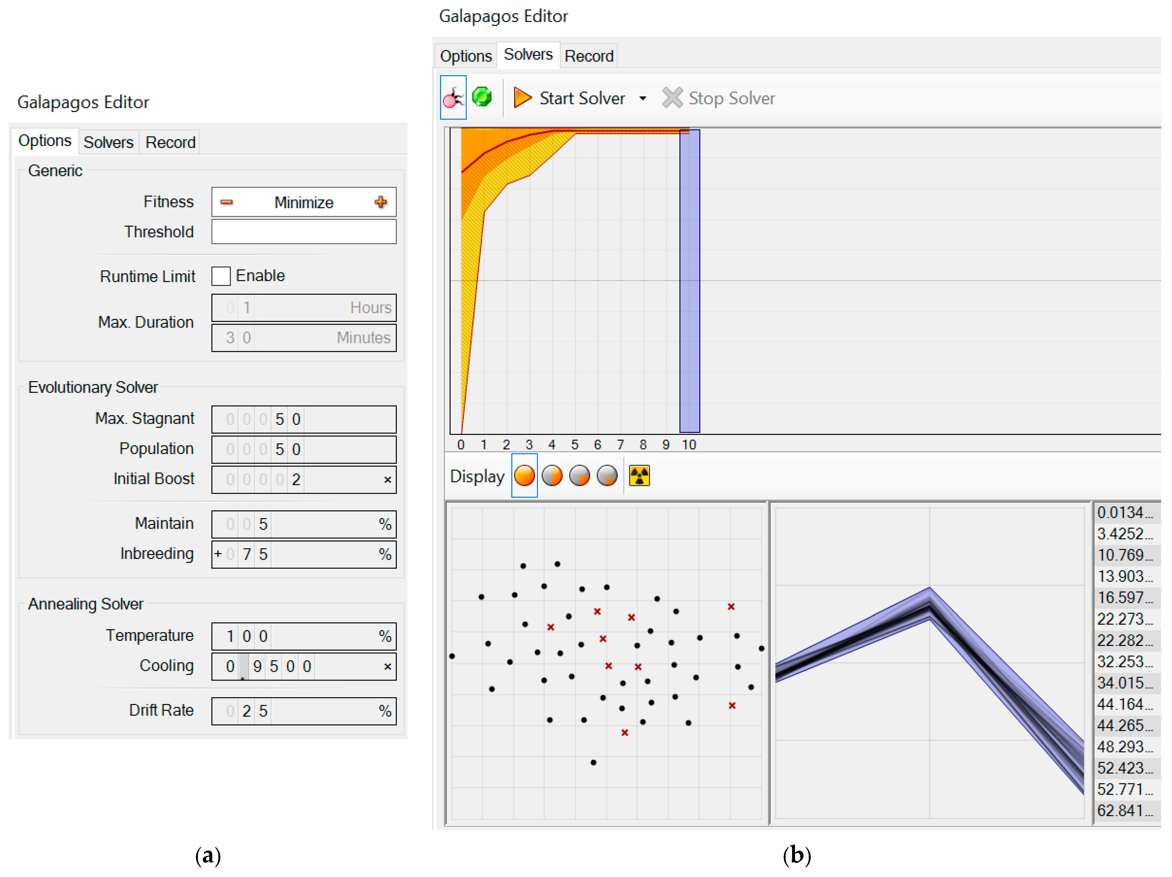
• To support the search for optimal solutions using artificial intelligence, including parametric artificial neural networks and optimizing genetic algorithms, due to the large number of independent and dependent variables and the complexity of the observed relationships between the properties of the models used;
• To automate the activities in the field of simulations, analysis and description of the existing relationships as well as predictions of the thermal operation of buildings with buffer spaces using computer techniques.

The main objective of this article is to present a new method for describing the thermal performance of buildings with unconventional forms and built-in buffer spaces designed to constitute solar efficient corrugated façades, especially in cold periods of a moderate climate. The atypical form of the building’s shapes results from the fact that each buffer space has glazed walls parallel to the planes of the corrugated and insulated southern wall of the designed building and an inclined insulated roof that is an extension of the roof of the building.

The developed parametric quantitative thermal model makes it possible to analyze the influence of the unconventional forms of buildings with buffer spaces on their thermal performance. The analysis was carried out based on the results of the computer simulations using many diversified discrete models. In addition, the analysis was extended to the search for the simultaneous influence of other parameters related to material properties, azimuth, infiltration and ventilation on the thermal performance of these buildings.

2. Methodology

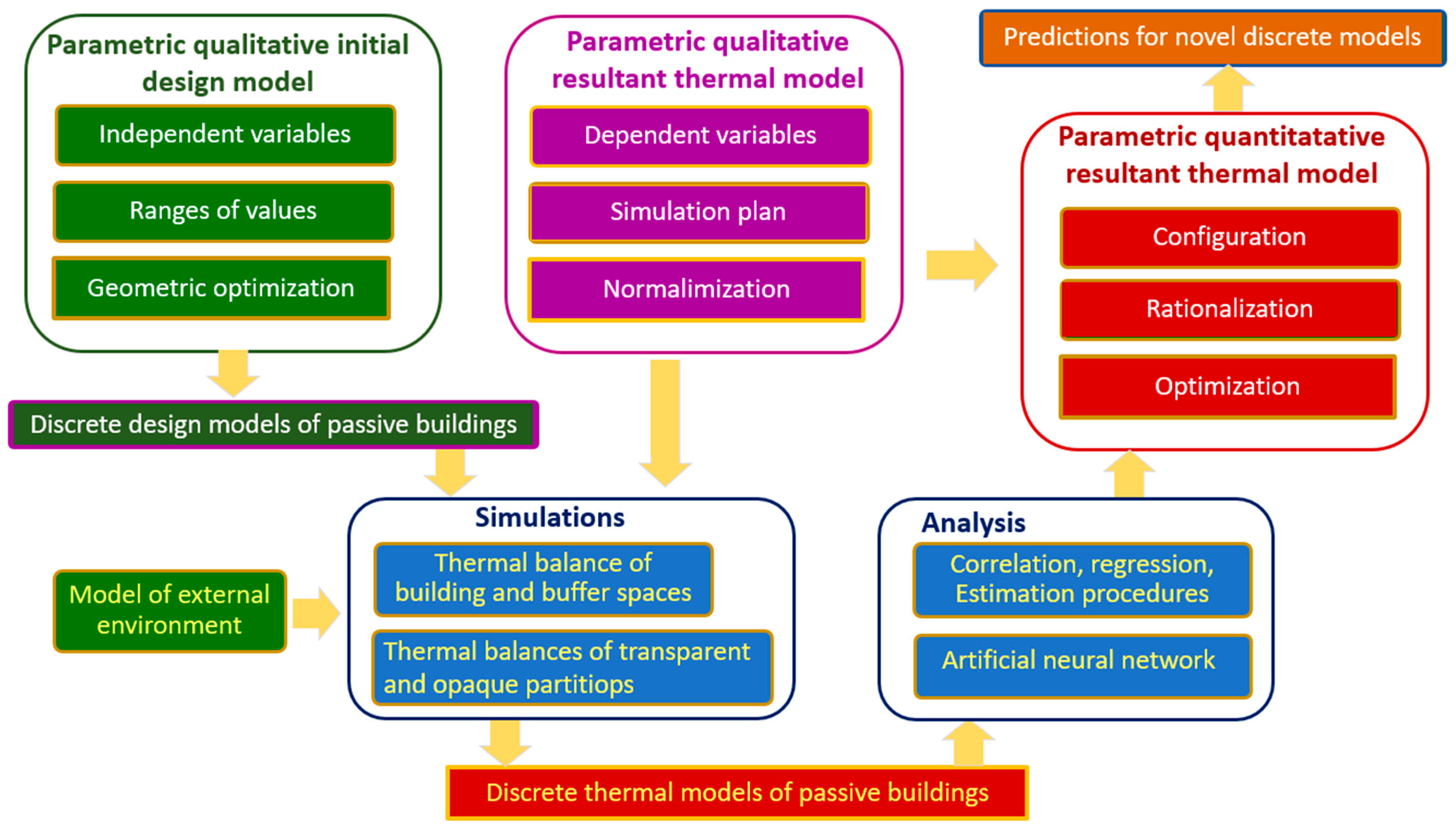
2.1. The Method’s Algorithm

The algorithm of the new method consists of five basic steps. The result of each step is a qualitative or quantitative model of a building with a buffer space employed in the next step. In the first step, a parametric qualitative physical model was created to define many discrete design models used in simulations, as shown in Figure 1. Thus, as a result of adopting a set of specific discrete values of various input parameters, the above-mentioned qualitative parametric model was used to define one discrete model of a building with a buffer space employed during one thermal simulation.

In the second step, a parametric qualitative thermal output model of buildings with buffer spaces was created to define the output parameters whose values are the results of the thermal simulations. The values of the dependent variables calculated during the simulations were assigned to the values of the input independent variable by means of this model. Thus, ten independent variables defining a few groups of parameters describing the geometric and physical properties of buildings with buffer spaces and five dependent variables defining the thermal performance of the buildings were used.

In the third step, a number of computer simulations using the discrete design models were performed to configure the qualitative parametric thermal model defined in the second step. Many discrete thermal models of passive buildings with buffer spaces were the result of this step. They related the set of the arbitrary input values of the independent variables with the set of the calculated output values of the resulting dependent variables. Because of the relatively large number of variables, discrete models and simulations, an automation of the calculations and file recording was introduced and supported by computer technology. Various tools offered by the Rhino/Grasshopper program [56] were used to perform a number of computer simulations. On the other hand, the tools offered by the Statistica program [57] were used to elaborate the parametric description of the observed relations and to search for new effective solutions using the implemented parametric artificial neural network.

The results of each step were automatically saved in an Excel spreadsheet [58]. In the fourth step, the relationships found between independent and dependent variables in this research were analyzed. Based on this analysis, the parametric qualitative thermal model created in the second step was configured to define a resultant parametric quantitative thermal model of buildings with buffer spaces. Thus, in the fifth step of the method’s algorithm, the resultant parametric quantitative thermal model was created using a number of various correlation, linear regression and nonlinear estimation procedures.

Because these procedures did not lead to satisfactory accuracy of the calculations, the method assisted in creating a parametric neural network meeting the required accuracy. In the additional last step, the method allowed predictions on a number of the effective discrete thermal models of buildings with buffer spaces, which were not created during the simulations and which fit within the assumed ranges of variability of the independent variables, guaranteeing the expected accuracy.

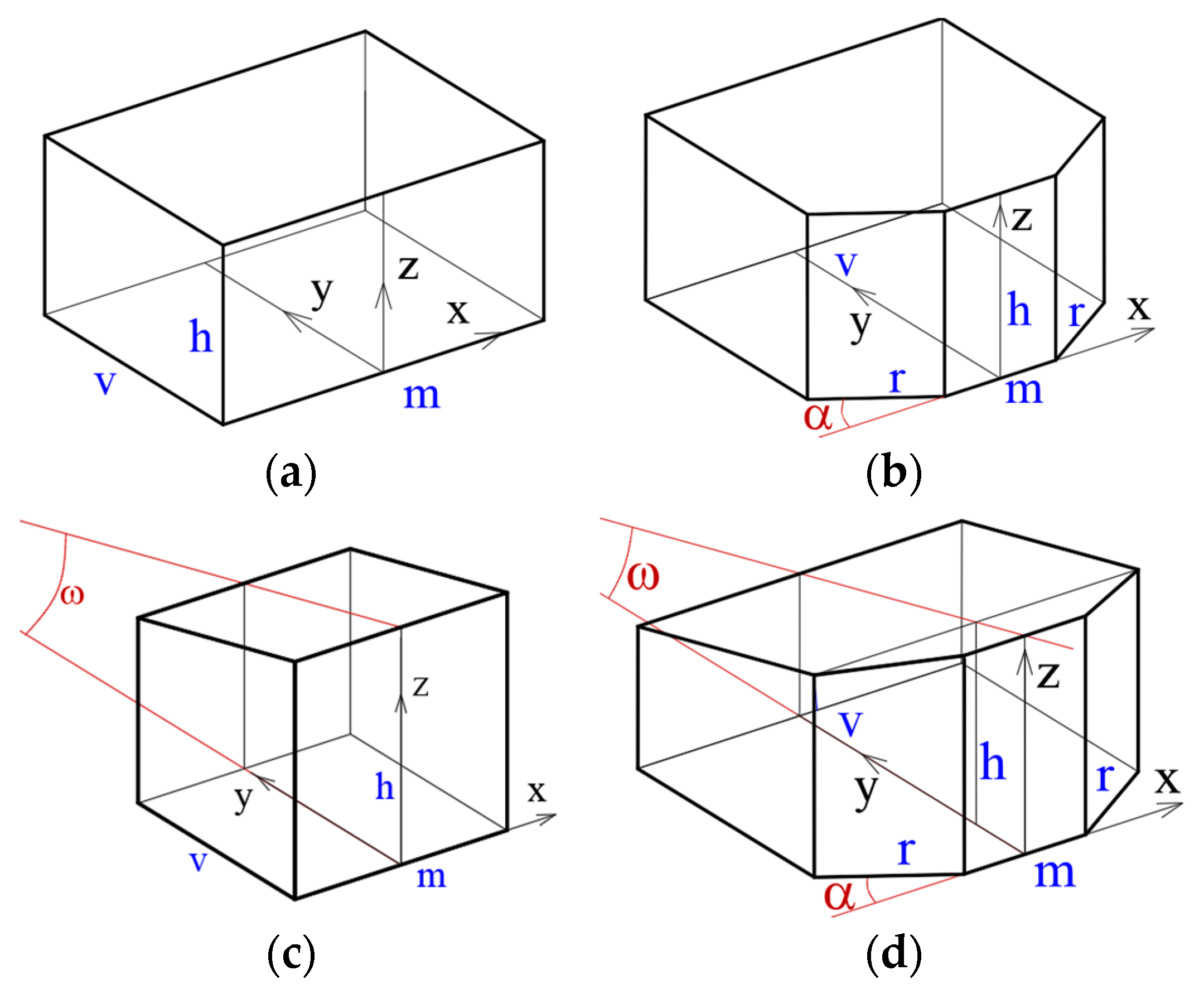
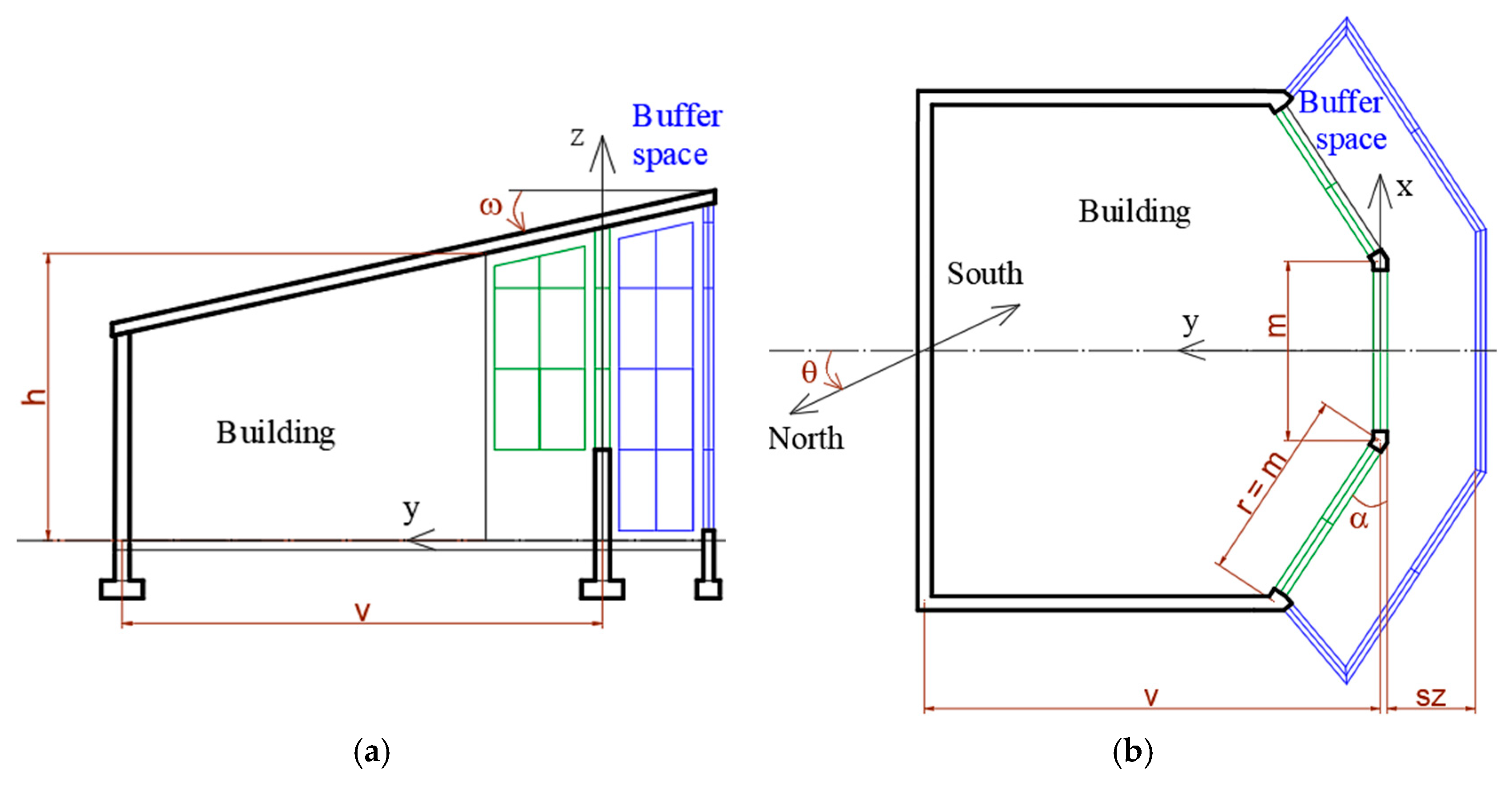
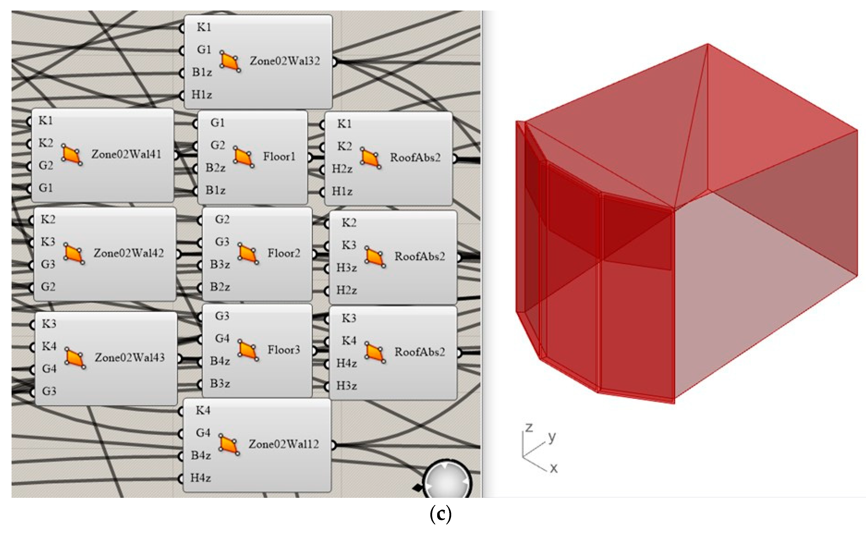
2.2. Geometric Models

The parametric qualitative design model created in the first step of the method’s algorithm was employed to create four types of building forms, as shown in Figure 2a–d. The basic cuboid form is presented in Figure 2a. The remaining forms were derived from the cuboid. These are (a) prismatic forms (see Figure 2b); (b) trapezoidal forms, as shown in Figure 2c; and (c) unconventional polyhedral forms (see Figure 2d). Thus, the input parameters defining the above forms are the reference height, h, and the length, v, of a building; the widths, r and m, of the southern wall strips; the angle α of the folding of the southern wall and the angle ω of the roof’s horizontal inclination.

To limit the variety of building forms to a reasonable number and to obtain a simple comparison between the created discrete models, the following three boundary conditions were adopted. The cubature V_ref of each considered form is equal to 3024 m³. The surface area P_cref of the envelope of each considered building is 1020 m². The area of the folded southern elevation wall of each building is equal to 168 m² or 210 m². The overall dimensions of the basic form can be calculated using Equations (1a)–(1c).

$${\mathrm{V}}_{\mathrm{r}\mathrm{e}\mathrm{f}}=\mathrm{v}·\mathrm{m}·\mathrm{h}=3024$$

(1a)

$${\mathrm{P}}_{\mathrm{c}\mathrm{r}\mathrm{e}\mathrm{f}}=2·\left(\mathrm{m}+\mathrm{v}\right)·\mathrm{h}+\mathrm{m}·\mathrm{v}=1020$$

(1b)

$${\mathrm{P}}_{\mathrm{r}\mathrm{e}\mathrm{f}}=\mathrm{m}·\mathrm{h}=168\mathrm{or}210$$

(1c)

The remaining dimensions of each derivative form must be adopted at the beginning of the calculations as the values of other independent variables. In the case of the form presented in Figure 2d, the values of two independent variables, ω and α, were selected from the predicted ranges of their variability. The values of the output parameters (the dependent variables) m, r, h and v (in meters) were calculated based on Equations (2a)–(2d).

$$F_{Vref}(\mathsf{\alpha },\mathsf{\omega },\mathrm{m},\mathrm{r},\mathrm{h},\mathrm{v})=V_{ref}$$

(2a)

$$F_{Pcref}(\mathsf{\alpha },\mathsf{\omega },\mathrm{m},\mathrm{r},\mathrm{h},\mathrm{v})=P_{cref}$$

(2b)

$$F_{Pref}(\mathsf{\alpha },\mathsf{\omega },\mathrm{m},\mathrm{r},\mathrm{h},\mathrm{v})=P_{ref}$$

(2c)

$$m=r$$

(2d)

To calculate the sets of values of the parameters m, v and r defining the subsequently simulated models, an optimizing computer program named Galapagos using genetic algorithms was implemented in the Rhino/Grasshopper application. This program iteratively calculated the values of m, h and v so that the sum of the squares of the differences between the values assumed for V_ref, P_{c_ref} and P_ref, and those calculated in the subsequent iterations, was as small as possible while maintaining the required accuracy of the calculations. The initial values of m, h and v are given intuitively at the beginning. The boundary conditions and values loaded into the program are presented in Figure 3. The operation of the program is not the main topic of this article, so it is not discussed in detail.

The form of each buffer space was adapted to the form of a building so that (a) the plane of the building roof was also the plane of the roof of the buffer space and (b) the planes of each glazed southern wall of the buffer space were parallel to the planes of the building (see Figure 4a,b). The only independent variable related to buffer spaces was their width, constant over the entire width and height of the southern elevation.

2.3. Physical Design Model

The developed parametric geometric model was extended to include the physical properties of a building and buffer space related to materials of all transparent and opaque partitions and arbitrary ventilation and infiltration. Thus, ten independent variables were adopted. Three of them were geometric variables, namely a, w and sz, defined in the previous section. The remaining independent variables were as follows: (1) the variable pb, defining the surface area of the southern wall; (2) the variable gwb, defining the ratio of the window area to the southern wall area; (3) the variable ot, representing the azimuth of the building; (4) the variable tp, defining a certain group of parameters related to the thickness of the thermal insulation of the roof, the thickness of the thermal insulation of the façade walls and the thickness of the concrete of the floor; (5) the variable pwb, defining the physical properties of the glass panels of each building such as thickness, transmissivity, emissivity and conductivity; (6) the variable pws, defining the physical properties of the glass panels of the buffer space related to their thickness, transmissivity, emissivity and emissivity back; and (7) the variable ivb, defining the ventilation and infiltration of the building.

Because of the relatively large number of simulations and the discrete physical models used to obtain satisfactory accuracy of the conducted calculations, the number of employed values of the independent variables was limited to two, as shown in

Table 1. The values of ten independent variables adopted for the designed discrete models employed in the simulations.

Type	Independent Variable	Set1	Set2
Geometric Model	ω	0°	12°
	α	0°	30°
	pb	168 m2	210 m2
	gwb	0.3	0.885
Material Model	tp	25 cm	35 cm—roof
		15 cm	25 cm—walls
		10 cm	30 cm—floor
	pwb	0.003 m	0.004 m—pane thickness
		0.88 W/m-K	0.88 W/m-K—transmittance
		0.85 W/m-K	0.88 W/m-K—emissivity
		1.0 W/m-K	0.70 W/m-K conductivity
Buffer Space Model	sz	3 m	0.5 m
	pws	0.003 m	0.004 m—pane thickness
		0.70 W/m-K	0.95 W/m-K—transmittance
		0.50 W/m-K	0.25 W/m-K—emissivity front
		0.50 W/m-K	0.25 W/m-K—emissivity back
Physical Model	ivb	0.00236/person	0.001180/person—ventilation
		0.00030/m2	0.000152/m2—ventilation
		0.000226/m2	0.000113/m2—infiltration
	ot	0°	−40°

.

The HVAC system operating in the building space and the range of the internal air temperature <20°, 25°> were adopted. Roller shades with 15 mm insulation that turn on every night when the temperature drops below 17° were also exploited. The above level of temperature was obtained as a result of an optimizing process. The values of the basic constants used during the simulations are given in

Table A1. The internal gains.

Type	Personnel Density [People/m2]	Lighting Power Density [W/m2]	Power Density of Equipment [W/m2]
	0.108	4.6	10.8

,

Table A2. The structure of building partitions.

External Wall	Layer	Value [mm]
South-facing external wall	Plaster	10
	Thermal insulation	Variable
	Concrete	400
	Cement–lime mortar	15
External wall (east-facing, north-facing, west-facing)	Plaster	10
	Thermal insulation	Variable
	Concrete	200
	Cement–lime mortar	15
Roof	Steel trapezial sheets	0.1 Variable 350 15
	Thermal insulation
	Reinforced concrete beam-slab cement–lime mortar
Floor	Concrete	100
	Thermal insulation	Variable
	Cement mortar	30
Triple-glazed windows	Pane1	Variable
	Argon	13
	Pane2	Variable
	Air	13
	Pane3	Variable

and

Table A3. The structure of the buffer space’s partitions.

Element	Layer	Value
South-facing external wall	Plaster	10 [mm]
	Thermal insulation	Variable
	Concrete	200 [mm]
	Cement–lime mortar	15 [mm]
Single-glazed windows	Thickness	4 [mm]
	U-value	[W/m·K]
	Solar transmittance	0.95
	Solar reflectance	0.04
	Emissivity	0.25
	Solar diffuse	No

in Appendix A.

The values of the parameters defining the external loads were downloaded from websites published by the ground meteorological stations and satellites [59,60]. The downloaded data concern a site near Rzeszow located in the Central European Plain. Its geographical coordinates are 50.07 N and 22.01 E, and the sea level is 300 m. The total gains ${\mathrm{Q}}_{\mathrm{s}\mathrm{o}\mathrm{l}}$ [kWh] resulting from the solar irradiation falling on the building envelopes were calculated with the help of the ASHARE tau model based on the Muneer model using Equation (3) [61,62].

$${\mathrm{Q}}_{\mathrm{s}\mathrm{o}\mathrm{l}}=\mathsf{\alpha }·\left({\mathrm{I}}_{\mathrm{b}}·\mathrm{c}\mathrm{o}\mathrm{s}\left({\displaystyle \frac{{\mathrm{S}}_{\mathrm{s}}}{\mathrm{S}}}\right)+{\mathrm{I}}_{\mathrm{s}}{·\mathrm{F}}_{\mathrm{s}\mathrm{s}}+{\mathrm{I}}_{\mathrm{g}}{·\mathrm{F}}_{\mathrm{s}\mathrm{g}}\right)$$

(3)

where α—the solar absorptance of the respective surface; S [m²]—the area of the irradiated surface; S_s [m²]—the sunlit area; I_b [kWh/m²]—the intensity of beam (direct) radiation; I_s [kWh/m²]—the intensity of sky diffuse radiation; I_g [kWh/m²]—the intensity of ground-reflected diffuse radiation; F_ss—the angle factor between the surface and the sky; F_sg—the angle factor between the surface and the ground.

2.4. The Research Plan

On the basis of the qualitative parametric design and thermal models, as shown in Figure 1, a simulation plan was elaborated using the Monte Carlo method [63] based on a random selection of one of two values of all adopted independent variables given in Table 1. The values of these variables were normalized to 0 and 1 to compare the strength of the correlations between each independent variable and the resultant thermal model. The value 0 after normalization was assigned to each independent variable belonging to Set1; see Table 1 and

Table 2. The normalized values of ten renamed independent variables defining the first ten discrete design models named the Cfgi configurations.

Config.	g_al	g_om	g_sz	g_tp	g_ot	g_pb	g_wb	v_ivb	p_wb	p_ws
Cfg1	1	1	1	0	1	1	1	1	1	1
Cfg2	0	0	0	0	1	1	0	1	0	0
Cfg3	0	0	0	0	1	1	1	1	0	0
Cfg4	1	0	1	1	0	1	0	1	1	0
Cfg5	0	1	1	1	1	1	1	1	1	0
Cfg6	0	0	1	1	1	0	1	0	1	0
Cfg7	1	1	0	1	0	0	1	0	0	0
Cfg8	1	1	1	0	0	1	0	0	0	0
Cfg9	1	1	0	0	0	0	1	0	1	0
Cfg10	0	1	1	0	1	1	1	0	0	0

. The value of 1 as the normalized value was assigned to each independent variable belonging to the Set2 column of Table 1. After normalization, the independent variables were denoted as g_al, g_om, g_sz, g_tp, g_ot, g_pb, g_wb, v_ivb, p_wb and p_ws. Their normalized values calculated for the first ten simulated configurations, Cfgi, are given in Table 2. In the first column of this table, the names of the first ten configurations are shown.

2.5. Parametric Thermal Model

The thermal performance of passive buildings with buffer spaces was simulated with the help of 343 discrete design models to configure the parametric thermal model defined in the second step of the method’s algorithm. Five dependent variables defining the resultant parametric thermal model were defined. The first variable E_tot is a sum of the heating and cooling energy. The solar radiation energy E_sol is the second dependent variable. The last three dependent variables, h, m and v, are related to the adopted geometric boundary conditions.

Based on the simulation results related to the discrete design and thermal models, an analysis of the relationships found between these models was carried out. This analysis primarily concerned a description of the relationships between the independent and dependent variables of these models. The relationships were determined during the simulations using building heat balances.

In the heat balance calculations, the quasi-stationary 3rdOrderBackwardDifference method based on the so-called Conduction Transfer Functions was used [47]. The method consists of iterative calculations performed in intervals four times shorter than one hour. In each subsequent iteration, some results selected from a few previous iterations are taken into account.

For the subsequently performed simulations and the discrete design models, thermal balances based on Equation (4) were cyclically executed.

$${\dot{Q}}_{za}={\dot{Q}}_i+{\dot{Q}}_{cnv}+{\dot{Q}}_{izn}+{\dot{Q}}_{inf}+{\dot{Q}}_{sys}$$

(4)

The definitions of the individual components of Equation (4) are as follows. ${\dot{\mathrm{Q}}}_{\mathrm{z}\mathrm{a}}$ is the thermal energy stored in an internal air and partitions; ${\dot{\mathrm{Q}}}_{\mathrm{i}}$ is the sum of the convective internal loads; ${\dot{\mathrm{Q}}}_{\mathrm{c}\mathrm{n}\mathrm{v}} \mathrm{i}\mathrm{s}$ the convective heat transfer from the internal space surfaces; ${\dot{\mathrm{Q}}}_{\mathrm{i}\mathrm{z}\mathrm{n}}$ is the heat transfer due to interzone air mixing between the building and its buffer space; ${\dot{\mathrm{Q}}}_{\mathrm{i}\mathrm{n}\mathrm{f}}$ is the heat transfer due to infiltration and ventilation of outside air; and ${\dot{\mathrm{Q}}}_{\mathrm{s}\mathrm{y}\mathrm{s}} \mathrm{i}\mathrm{s}$ the air system energy provided to the internal space. All quantities were measured in [kWh]. The air system delivers hot and cold air to the internal space to meet heating or cooling requirements.

The heat balance of each outside surface is given by

$${\dot{q}}_{sol}+{\dot{q}}_{thr}+{\dot{q}}_{outcv}-{\dot{q}}_{cd}=0$$

(5)

The meaning of the individual components is as follows: ${\dot{q}}_{sol}$ is the absorbed solar radiation heat flux; ${\dot{q}}_{thr}$ is the long wavelength (thermal) radiation flux exchange between the internal space and surrounding space; ${\dot{q}}_{outcv}$ is the convective flux exchange with outside air; and ${\dot{q}}_{cd}$ is the conduction heat flux into the wall. All quantities were measured in [kWh/m²].

3. Simulation Results

A total of 343 simulations of the thermal operation of passive buildings with buffer spaces were carried out by means of the subsequent discrete Cfgi configurations. The simulations were performed with the conformity of the stochastic plan. Thus, 343 sets of values of five dependent variables defining the resultant discrete thermal models were calculated. The values of these dependent variables corresponding to the first ten exemplary Cfgi configurations are presented in

Table 3. The values of the dependent variables defining the first ten discrete thermal models, Cfgi.

Config.	Etot kWh/m2	Esol kWh/m2	r = m [m]	v [m]	h [m]
Cfg1	35,237	151,907	4.59	18.80	14.94
Cfg2	44,605	125,467	5.69	14.40	12.30
Cfg3	44,686	125,457	5.69	14.40	12.30
Cfg4	34,211	108,652	4.84	16.58	14.47
Cfg5	23,455	103,295	5.09	16.51	13.74
Cfg6	44,071	813,989	4.67	18.00	12.00
Cfg7	65,172	131,427	4.71	26.35	11.55
Cfg8	68,890	109,515	4.59	18.80	14.94
Cfg9	66,304	131,427	4.71	26.35	11.55
Cfg10	65,035	103,295	5.09	16.51	13.74

.

A visualization of the simulated discrete Cfg8 configuration made in the Rhino/Grasshopper program is presented in Figure 5a. Several selected graphical elements of the programming code, called containers, employed to load the initial data values required during the simulation, are shown in Figure 5b. A building model of part of the computer program consisting of eleven containers defining eleven individual planes of a row is presented in Figure 5c (shown on the right).

4. The Analysis of the Simulation Results

In the first part of the analysis of the obtained simulation results, the correlation strength between all independent and dependent variables was examined to obtain initial information on the dependence between the initial parametric design model and the resultant parametric thermal model of the passive buildings with buffer spaces. In the second part, an analytical description of the dependencies found between the variables of the input design model and the output thermal model was sought. This description was made using analytical formulas with a particular emphasis placed on the expected accuracy. The search for these formulas was carried out in two phases. In the first phase, several linear dependencies and formulas were sought using linear regression procedures. In the second phase, various nonlinear regression procedures were employed to obtain the required accuracy. The level of significance of p < 0.05 was adopted to develop a quantitative description with the regression procedures.

In the third part of this analysis, several types of artificial neural networks were used because of the small accuracy of the obtained analytical formulas. The implemented new artificial neural network allowed for a fairly accurate elaborated quantitative description of the relations found during the simulations to be obtained.

The developed resultant parametric thermal model allows one to shape the effective thermal performance of passive buildings with buffer spaces in a moderate climate. Thus, in the last step of the analysis, the developed qualitative parametric thermal model and the neural network were employed to search for a number of rational passive buildings with buffer spaces characterized by effective thermal performance.

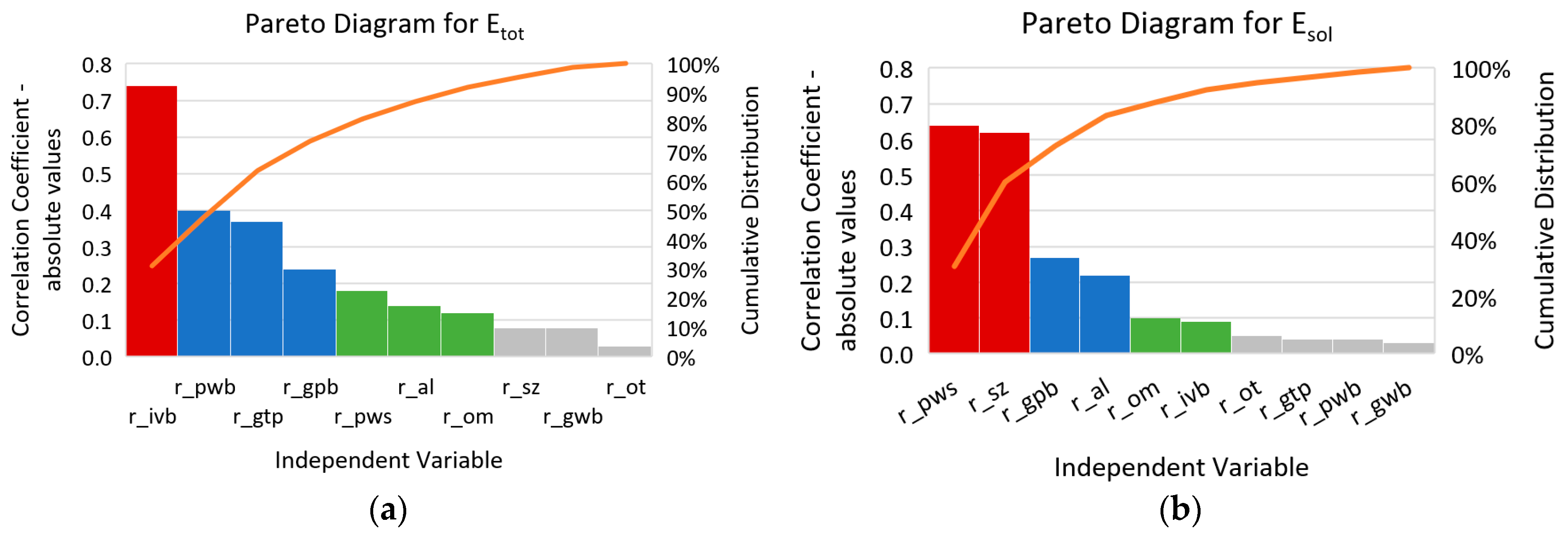
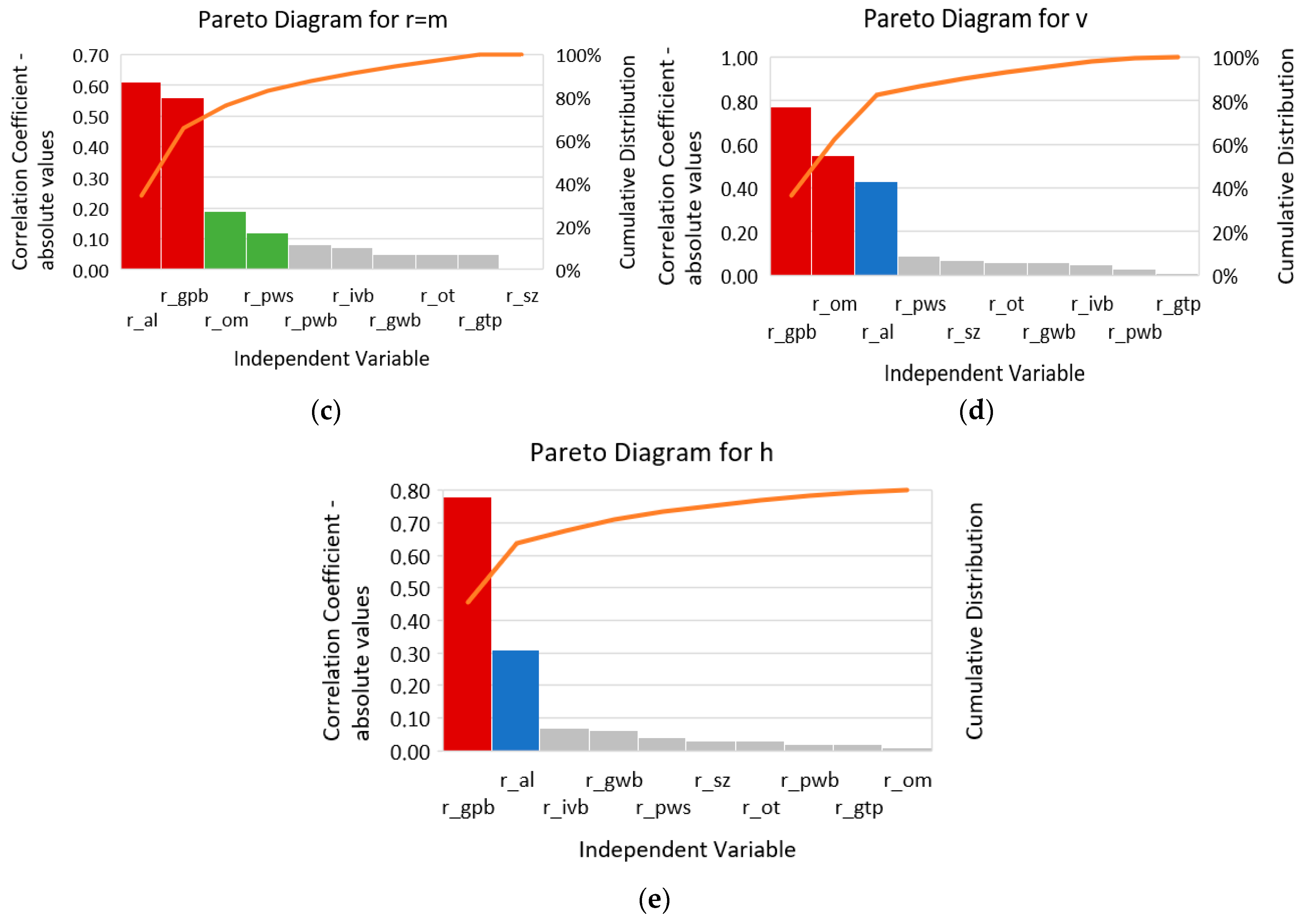
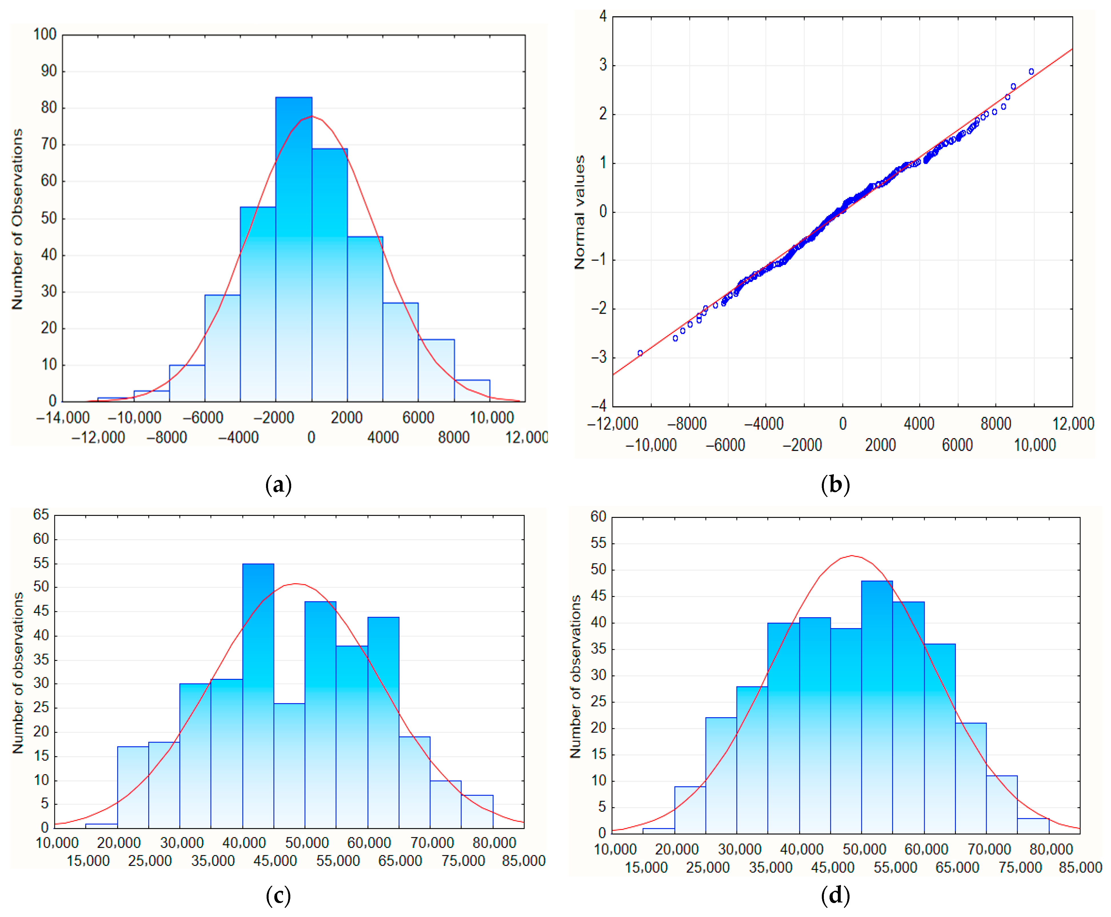
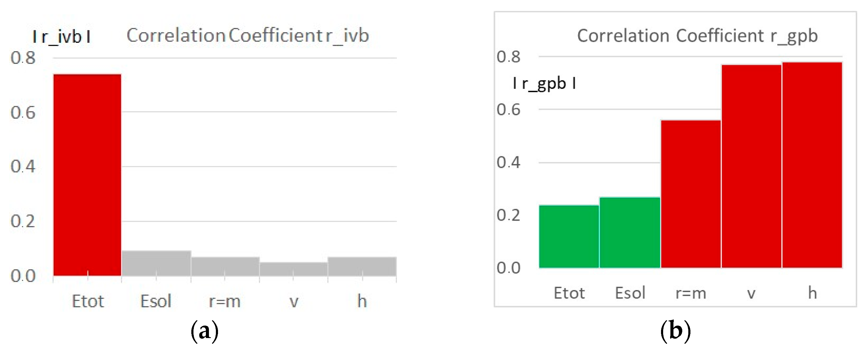
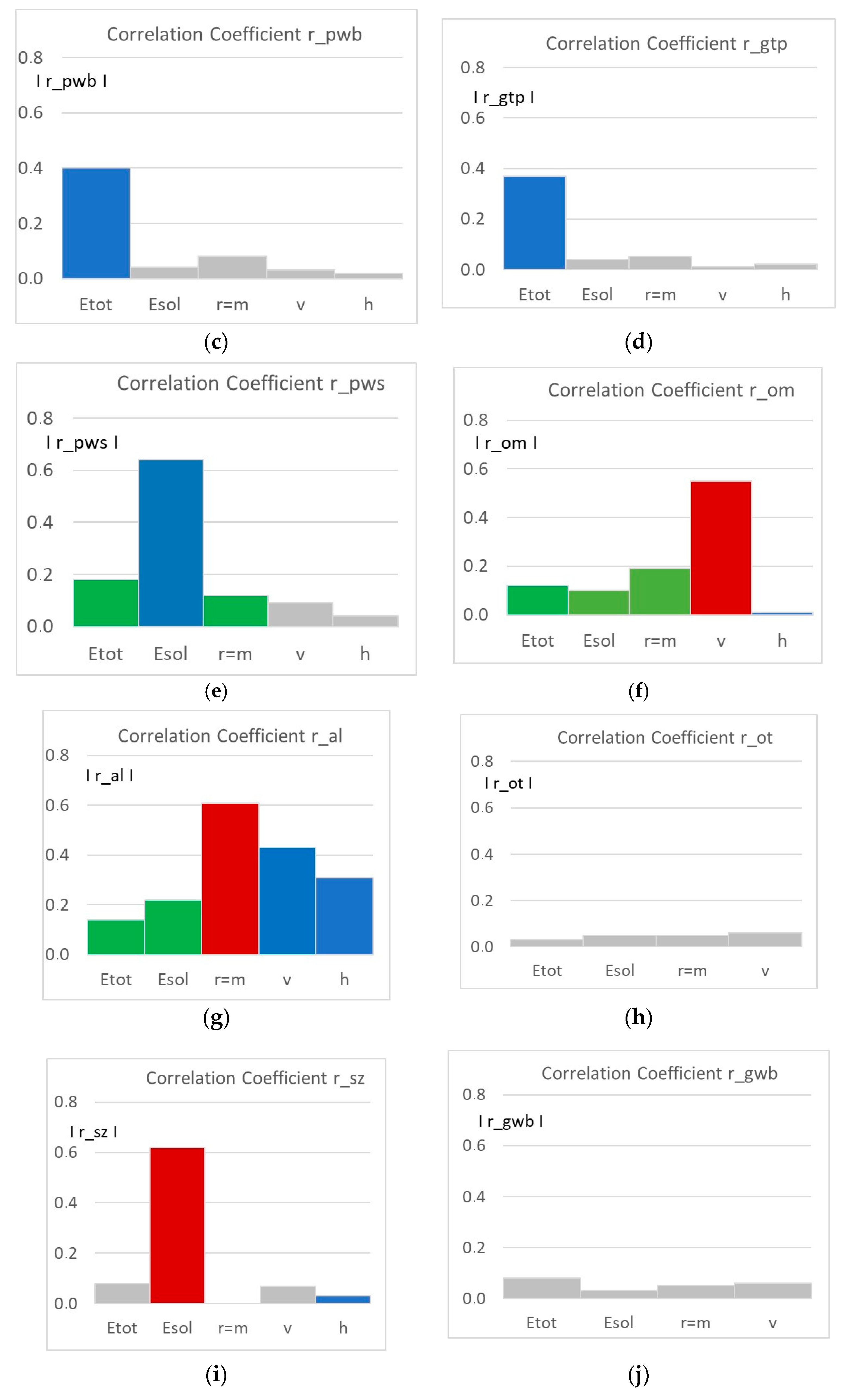
4.1. Correlation Analysis

To determine the dependence between the initial parametric design model and the resultant parametric thermal model, a few statistical procedures available in the Statistica computer program [57] were used. A basic parameter used to examine dependence was the correlation coefficient r(x_i). The correlations between all dependent and independent variables were found at the level of significance of p < 0.05. The calculated values of the correlation coefficients are given in

Table 4. The correlation coefficients between ten independent and five dependent variables of the parametric thermal model at the significance level p < 0.05.

Dependent Variable	Correlations
	r_al	r_om	r_sz	r_gtp	r_ot	r_gpb	r_gwb	r_ivb	r_pwb	r_pws
Etot	0.14	0.12	−0.08	−0.37	0.03	−0.24	−0.08	−0.74	−0.40	−0.18
Esol	0.22	0.10	−0.62	−0.04	−0.05	0.27	0.03	0.09	0.04	0.64
r = m	−0.61	−0.19	0.00	0.05	0.05	0.56	0.05	0.07	−0.08	−0.12
v	0.43	0.55	−0.07	0.01	−0.06	−0.77	0.06	−0.05	0.03	0.09
h	0.31	−0.01	0.03	−0.02	0.03	0.78	−0.06	0.07	0.02	−0.04

. If the value of r(x_i) is close to 1 or −1, then correlations are very strong. A negative value of this coefficient close to −1 indicates an inversely proportional correlation between the respective independent and dependent variables. To illustrate the obtained diversified strength of these correlations in an orderly manner, five diagrams, presented in Figure 5a–d, were developed. These diagrams were made with Excel [58].

A very significant impact of four independent variables, v_ivb, p_wb, g_tp and g_pb, on E_tot can be seen in Figure 6a. For each of these variables, the calculated absolute value of r(x_i) is greater than 0.2. In the case of three independent variables, g_ot, g_sz and g_wb, r(x_i) is less than 0.1. This fact indicates a lack of correlations between these variables and the thermal performance of the considered passive buildings with buffer spaces. The vertical axis placed on the right side of each diagram shows the percentage share of the subsequent independent variables in the impact on the thermal performance of the examined passive buildings with buffer spaces. It starts from approx. 25% of the v_ivb’s share (see Figure 6a), which can be read from the orange curve. The beginning not being very vertical, the uniformly changing slope and curvature of this line indicate steadily decreasing power of the correlation between x_i and E_tot.

In the second diagram, shown in Figure 6b, we can see that the correlations between two independent variables, p_ws and g_sz, and E_sol are very strong because the values of their coefficients are greater than 0.6. The big inclination of the starting fragment of the segment line points to a very strong magnitude of correlations between the first two variables and the thermal performance of the passive buildings. Therefore, we are able to deduce that the amount of solar energy E_sol delivered to the interior can be decisively influenced by the properties of the windows and the width of the buffer space. The strength of the correlations between g_pb or g_al and E_sol is temperate. The infiltration, ventilation and roof slope seem to have a relatively small impact on E_sol. The correlations between four variables, g_ot, g_tp, g_wb and p_wb, and E_sol can be negligible.

Two independent variables, g_al and g_pb, are strongly correlated with the third dependent variable, m (equal to r). The correlation between two independent variables, p_ws and g_om, and m is weak, as shown in Figure 6c. The remaining variables seem to be very weakly correlated with m.

The correlations between the dependent variable v and the same three variables are also strong; however, their strength is a little different than in the previous case (see Figure 6d). From the diagram, it follows that the impact of the size and magnitude of the southern wall’s corrugation as well as the roof slope on the building length, v, may be very strong with the high probability.

The correlations between the variables g_pb and g_al and the last dependent variable, h, are strong, as shown in Figure 6e. Thus, the size and corrugation of the southern wall should determine the building height h.

4.2. Regression Analysis

To elaborate an analytical description of the relations occurring between the parameters of the input parametric design model and the output parametric thermal models, a regression analysis was carried out. In the first phase of this analysis, a linear description of these relations was performed using Equation (6).

$${\mathrm{y}}_{\mathrm{k}}={\sum }_{i=1}^{10}\left(b_i·x_i\right)+b_0$$

(6)

The following symbols are used in Equation (6). y_k is the kth dependent variable; x_i is the ith independent variable; and b_i and b₀ are the searched constant coefficients that must be calculated with the help of the linear regression procedures [57]. The obtained values of b_i coefficients are shown in

Table 5. The regression coefficients calculated for five linear dependencies.

Coefficients Calculated for Etot, pc = 0.000, R = 0.96, R2 = 0.93
b0	b1	b2	b3	b4	b5	b6	b7	b8	b9	b10
69,566	3271	46,678	−1666	−10,573	695	−4105	−3150	−19,001	−10,273	−40,079
Coefficients calculated for Esol, pc = 0.000, R = 0.96, R2 = 0.93
b0	b1	b2	b3	b4	b5	b6	b7	b8	b9	b10
112,833	17,342	4213	−4286	−984	−4501	29,453	−1482	−493	1127	49,965
Coefficients calculated for r = m, pc = 0.000, R = 0.81, R2 = 0.65
b0	b1	b2	b3	b4	b5	b6	b7	b8	b9	b10
4.984	−0.420	−0.100	−0.042	0.0354	0.002	0.354	0.047	0.021	−0.028	−0.059
Coefficients calculated for v, pc = 0.000, R = 0.98, R2 = 0.95
b0	b1	b2	b3	b4	b5	b6	b7	b8	b9	b10
18.826	2.681	3.799	−0.177	0.155	0.017	−5.446	0.213	0.072	−0.158	−0.145
Coefficients calculated for h, pc = 0.000, R = 0.87, R2 = 0.76
b0	b1	b2	b3	b4	b5	b6	b7	b8	b9	b10
11.251	0.952	0.096	0.108	−0.100	0.006	2.022	−0.122	−0.077	0.083	0.150

.

The modeling accuracy obtained using Equation (6) and the above regression coefficients was very low and unacceptable. Although the explained variance R² seems quite attractive, as shown in

Table 6. The results obtained for the first ten Cfgi configurations with the help of the regression analysis.

Configuration	Calculated Values of Etot kWh/m2	Predicted Values of Esol Linear Regression kWh/m2	Residuals	Predicted Values of Esol Neural Network kWh/m2	Residuals
Cfg1	35,237	35,708	−471	35,439	−203
Cfg2	44,605	47,138	−2533	44,635	−30
Cfg3	44,686	44,041	645	44,775	−89
Cfg4	34,211	27,142	7069	34,349	−138
Cfg5	23,455	26,104	−2649	22,771	685
Cfg6	44,071	44,684	−613	43,834	238
Cfg7	65,172	63,905	1267	65,189	−17
Cfg8	68,890	71,639	−2751	68,893	−3
Cfg9	66,304	64,108	2196	66,613	−309
Cfg10	65,035	65,980	−945	65,065	−30

, and the obtained distributions confirm the correctness of the calculations (see Figure 7a–d), the dispersion of the obtained results within the limits ± 20% of the values obtained during the simulations does not meet the requirements, e.g., the value of 7069 from the fourth column of Table 6.

In the second phase, a number of nonlinear formulas were taken into account to describe the influence of the independent variables on the resultant model with the help of various nonlinear regression and estimation procedures to maintain the expected modeling accuracy. The obtained results did not improve the accuracy of the previously obtained analytical description of the thermal performance of the passive buildings with buffer spaces.

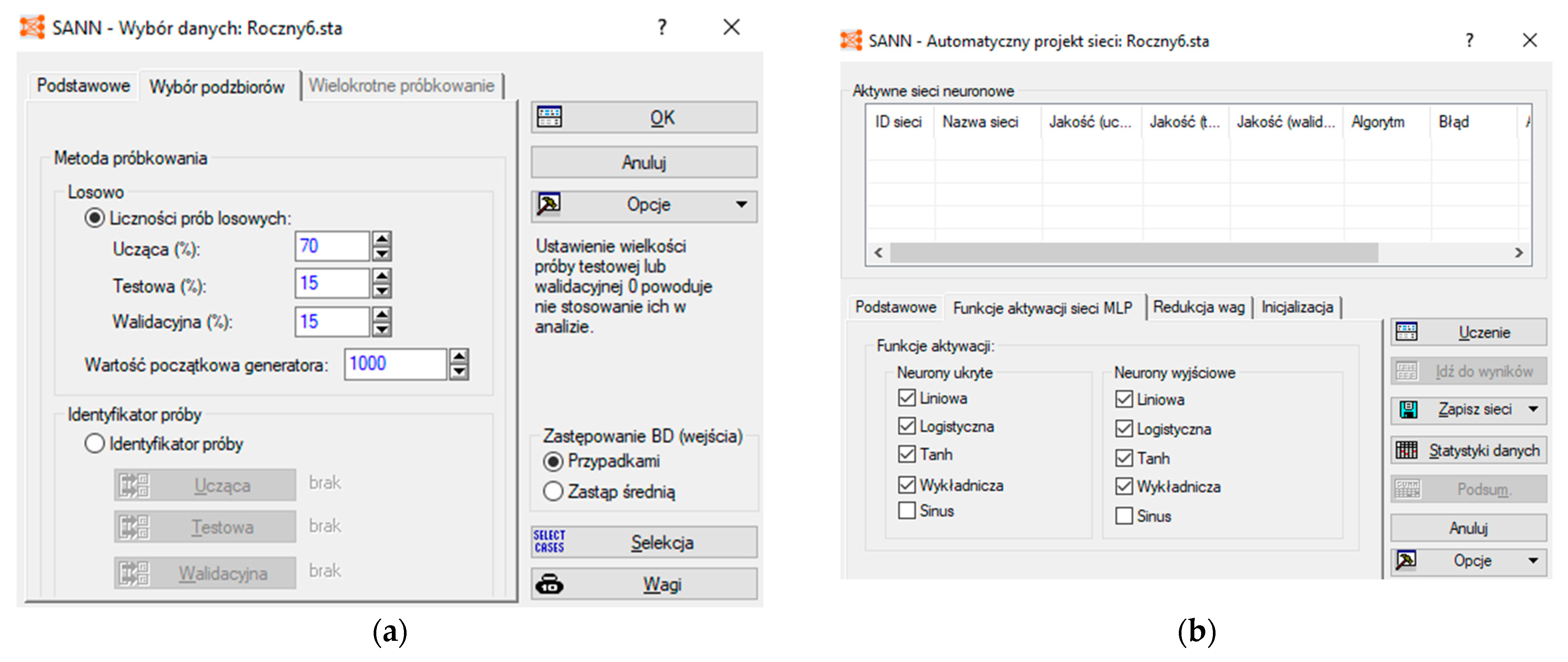
4.3. The Parametric Neural Network Describing the Relations Found During the Simulations

The relatively large number of independent and dependent variables and the impossibility of obtaining a satisfactory description of the relations between these variables with the regression methods forced the search for an artificial neural network meeting the required accuracy. It was assumed that the new neural network must ensure that the differences between the calculated values and the values obtained during the simulations should not exceed ±3.5%. To determine the accurate artificial neural network, the automatic option provided by the statistics computer package Statistica [57] was selected.

The optimal MLP type of artificial neural networks with the BFSG learning algorithm (coming from the names of its authors, Broyden, Fletcher, Goldfarb and Shanno) was selected due to its high quality of learning, testing and validation. The BFGS algorithm belongs to the family of quasi-Newtonian algorithms based on the finite differences in gradient approximations of objective functions [59].

The implemented optimal neural network, MLP 10-25-5, is based on three hidden layers. The first layer consists of 10 neurons, the second consists of 25 hidden neurons and the last layer consists of 5 neurons. The network was selected from a lot of standardized networks because it is characterized by (1) very high values of training, testing and validation quality coefficients that are equal to 0.99997, 0.99987 and 0.99991, respectively, and (2) symmetric normal histograms of the E_tot’s values and residuals; see Figure 8a–d.

These results indicate a fairly high accuracy of the developed neural network. This neural network has a correct normal distribution of the residuals resulting from the stochastic simulation plane, as shown in Figure 8a,b. Additionally, the histogram of the values calculated using the network is almost identical to the histogram of the values obtained during the simulations, as shown in Figure 8c,d. The network is characterized by the 744 BFSG learning algorithm, a logistic input function and a linear output function.

The input data were automatically divided using the Statistica program. To create the neural network, 70% of the input data was used to train the network, 15% was used for testing and 15% for validation. The functions used to find the properties of the neural network are shown in Figure 9a,b. The employed procedures allowed for satisfactory results in terms of the effective passive buildings with buffer spaces.

5. Discussion

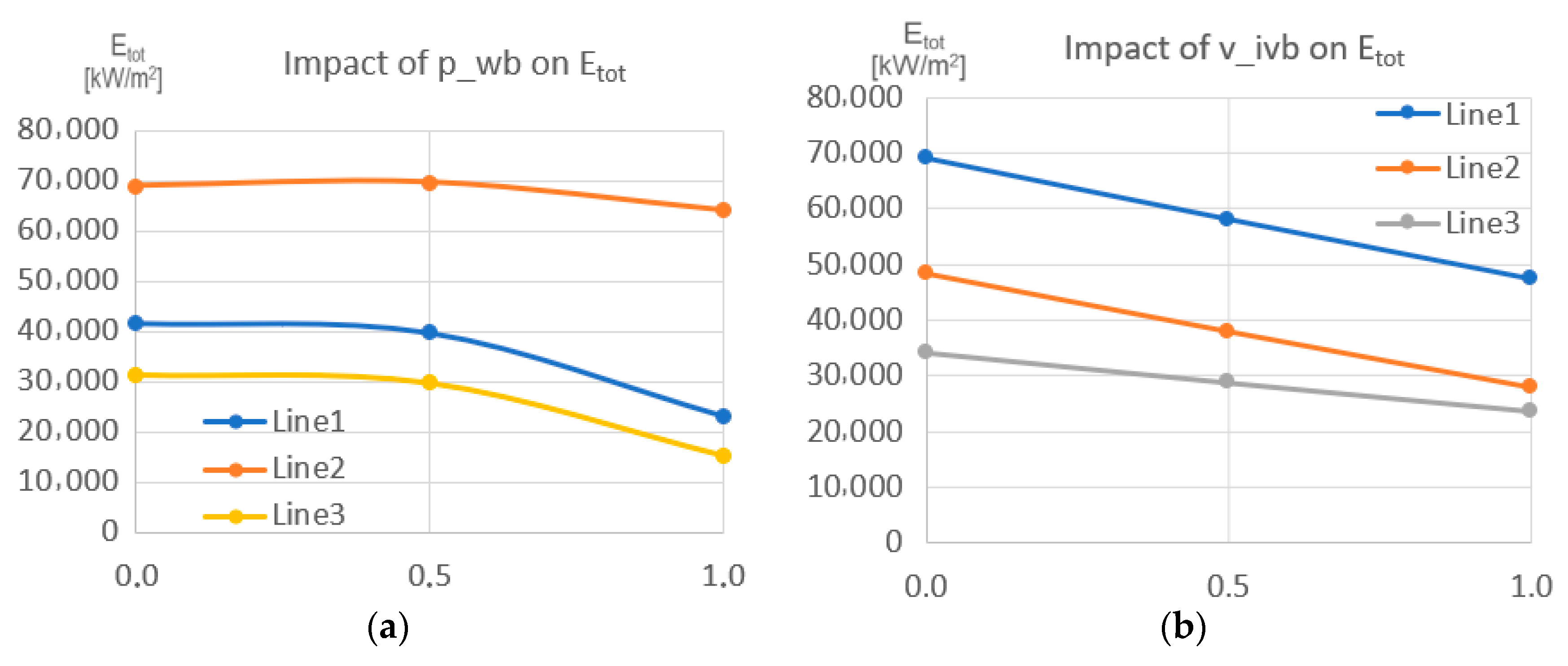
5.1. The Impact of Each Independent Variable on the Thermal Model of Buildings with Buffer Spaces

The diversified strength of the correlations between the individual independent variables and the resultant thermal model represented by the total energy E_tot can be seen in the diagrams presented in Figure 10a–j. The diagram in Figure 10a shows a very strong correlation between the v_ivb (ventilation and infiltration) and E_tot. The strength of the correlations between other dependent variables and E_tot is negligible.

The correlations between the independent variables p_wb and g_tp and E_tot are strong, as shown in Figure 10c,d. The correlations between four independent variables, g_pb, p_ws, g_om and g_al and, two dependent variables, E_tot and E_sol, are temperate; see Figure 10b,e–g. The correlations between three independent variables, g_ot, g_sz and g_wb, and the dependent variable E_tot are weak, as shown in Figure 10b,h–j. In the case of the independent variable g_sz, the correlation between this variable and E_sol is very strong, as shown in Figure 10i.

In the research, emphasis is mainly placed on searching for the relationships between the energy E_tot supplied to the building and the independent variables x_i of the design model. The influence of all independent variables on the remaining dependent variables of the parametric resultant thermal model of passive buildings with buffer spaces can be analyzed in a similar way.

The differences between the predicted values calculated using the elaborated neural network and the values obtained from the simulations are acceptable and amount to (a) 2 cm for the r (width), h (height) and v (length) of the buildings; (b) 600 kWh for the E_tot value regarding total heating and cooling energy; and (c) 2500 kW of gains from the solar irradiation falling on the building envelope. Thus, the obtained differences are up to 3.5%.

5.2. A Comparison of the Obtained Results with the Available Results from Other Studies

Several buildings with buffer spaces, the type, structure and function of which are most similar to those considered in this article, were analyzed by A. Vukadinović et al. [53]. The authors adopted ten parameters (independent variables) defining individual properties of the buildings and buffer spaces. They examined the influence of these parameters on the thermal performance of these buildings, mainly on the heating and cooling energy. These buildings are located in the Humid Subtropical Climate conditions occurring in Serbia in Central Europe.

Two independent variables, the façade glazing type and façade wall structure, analyzed by A. Vukadinović et al. [53], are considered to correspond to the independent variables g_pwb and g_tp with some approximation. The correlation between the above independent variables and the heating and cooling energy was found to be strong in both studies, i.e., the buildings analyzed by A. Vukadinović et al. and the buildings analyzed in this article. The correlation between the window-to-wall ratio of the south-facing façade and the heating and cooling energy was found to be insignificant in both studies as well. On the other hand, a moderate correlation between the physical properties of the windows of the buffer space was proven by A. Vukadinović et al., which also coincides with the analogous correlation strength observed between g_pws and E_tot in this paper.

The disadvantage of the research conducted by A. Vukadinović et al. is that they did not check the accuracy of the parametric model made with statistical methods, for example, using the explained variance R². However, the fundamental difficulties in comparing the results obtained in this work with the results of the research conducted by other researchers result from the fact that the independent variable v_ivb defining ventilation and infiltration was taken into account and the strength of its correlation with E_tot was high. The novelty of this work results, among other things, from the above-mentioned inclusion of ventilation and infiltration as a single independent variable.

A. Vukadinović et al. [54] analyzed the influence of the shape factor of a building with a glass buffer space attached to its south-facing elevation wall. However, the geometric, physical and thermal characteristics of their sunspaces differ from the characteristics of the buffer spaces analyzed in this article. First of all, the sunspace did not have a non-transparent insulating roof, side walls and floor. The buildings were also located in the humid subtropical climate occurring in Serbia in Central Europe. The authors proved a moderate influence of the building shape, i.e., the proportion between the overall dimensions of a building on the heating and cooling energy, which coincides with the moderate strength of the correlation found between the independent variables g_al, a_al, h, v and m. The novelty of this work also results from the above consideration of the roof pitch and the corrugation of the southern elevation as independent variables and the height, width and corrugation of the southern elevation as dependent variables.

The stochastic Monte Carlo method was used to elaborate the research plan based on the unordered selection of the arbitrary discrete values adopted for the independent variables. As a result, unordered sets of discrete values of the dependent variables defining the resultant thermal model were obtained. Based on these sets, it is fairly difficult to present the impact of changes in the values of the individual independent variables on the resultant model.

5.3. New Effective Configurations of Buildings with Buffer Spaces Based on the Parametric Quantitative Model

The resultant quantitative parametric thermal model based on the elaborated neural network led the authors to predict a number of subsequent discrete thermal models by changing the values of the subsequent independent variables in an ordered manner. This action allows one to create several diagrams illustrating the relationships between the independent and dependent variables defining the parametric design model and the resultant parametric thermal model.

The results of the ordered predictions are presented in two diagrams shown in Figure 11a-b. In the first case, the normalized values of the p_wb parameter were taken from the set {0.0, 0.5, 1.0} and measured on the abscissa axis in Figure 11a. In the second case, the discrete values of the v_ivb parameter were also taken from the above set; see Figure 11b.

The diagram presented in Figure 11a shows the diversified influence of the independent variable p_wb, representing the physical properties of the building windows, on the dependent variable E_tot depending on the values of other independent variables. The greater the slope of any of the lines (Line1, Line2 and Line3), the greater the influence of p_wb on E_tot. Line1 was determined for the values of the remaining independent variables equal to 0. The position and shape of Line1 indicate that the change in the value of the p_wb variable within the adopted variability range results in E_tot energy savings of approximately 10%. Line2 was obtained for the remaining independent variables equal to 1. Its position and shape indicate that the change in the value of the p_wb variable within the adopted variability range results in E_tot energy savings of approximately 55%. Line3 was determined for the diversified values of the remaining variables. In this case, the position and shape of Line3 indicate that E_tot energy savings can reach up to 50%.

The diversified positions of a buffer space relative to a building affecting the form and thermal performance of the building were analyzed by G. Yao et al. [34]. The authors analyzed the properties of fifteen different types of buildings with buffer spaces to select the type and number of parameters defining their models for computer simulations. The parameters whose influence was studied were the width of buffer space, the glazing type, the window-to-wall ratio, the external wall U-value and the roof U-value. The considered buildings were divided into three groups: trombe walls, sunrooms and ceiling-mounted buffer rooms. The first type was characterized by the fact that the examined buildings included cumulative walls. In this case, the heating and cooling energy gains were up to 14.5%. The second type was characterized by the fact that all roofs and walls were made of glass. In this case, the heating and cooling energy gains were up to 15%. In the third case, the buffer space was built into the building so it had opaque walls and a roof. In this case, the heating and cooling energy gains amounted to 53% depending on the geometric and physical properties of the opaque and transparent elements.

Of the three types of buffer spaces mentioned above, the sunspace is the most similar to the types of buildings with buffer spaces considered in this section because it is the southern glass façade of the building. This buffer space allows for savings in heating and cooling energy at the level of 15%, which is much less than 50%, resulting from Line3 shown in Figure 11a. This fact results from the arrangement of buffer spaces on the entire insulating elevation, the covering with an insulated roof, the insulated side walls and floor and the use of insulated movable roller sheds on the windows of the buffer space.

The accuracy of statistical modeling using neural networks is expressed by three coefficients: learning, testing and validation errors. In the case of the developed neural network MLP 10-25-5, these coefficients are greater than 0.999, and the distribution of the calculated residuals is normal, which indicates a very good fit of the developed MLP networks to the relations found during the simulations, as shown in Table 4. The obtained modeling accuracy is higher than that in the research presented in the Introduction, where the reported maximum modeling accuracy of the complex building without the buffer space was defined by the explained variance R² equal to 0.99. A similar analysis for buildings with buffer spaces was not performed.

Three lines, shown in Figure 11b, present a very strong influence of v_ivb on E_tot depending on the diversified values of the remaining variables. Line1 was obtained by the values of the remaining independent variables equal to 0. The position and shape of Line1 indicate that the change in the value of the v_ivb variable within the adopted variability range results in E_tot energy savings of approximately 30%. Line2 was achieved when the remaining independent variables were equal to 0 or 1. Its position and shape indicate that the change in the value of the v_ivb variable within the adopted variability range results in E_tot energy savings of approximately 42%. Line3 was obtained by the remaining independent variables equal to 1, except for the variable g_sz, whose value was equal to 0. In this case, the position and shape of Line3 indicate that E_tot energy savings can reach up to 50%. An important aspect of this research is therefore an innovative analysis of the impact of ventilation and infiltration, defining the single independent variable v_ivb, on the resultant parametric model of buildings with buffer spaces.

The above diagrams show a very significant impact of p_wb and v_ivb on E_tot. In the first case, the relative decreases in the value of E_tot range from 7% to 51% in relation to the initial value of E_tot obtained for p_wb and v_ivb equal to 0 depending on the values of other independent variables. In the second case, the decreases in the value of E_tot range from 31% to 43% depending on the different values of other independent variables, too.

To summarize, it can be stated that the results presented in this article are comparable with the results obtained by A. Vukadinović et al. [53] and G. Yao et al. [34]. The accuracy of the parametric modeling of the thermal performance of buildings with buffer spaces built into the southern elevation using the new method is comparable to that presented by H. Hosamo et al. [55] and sufficient for engineering purposes.

6. Conclusions

The elaborated new method of searching for a parametric description of the thermal performance of passive buildings with buffer spaces in a temperate climate is based on a new input parametric design model defined by 10 independent variables. This model supports the process of simulating the thermal performance of passive buildings with buffer spaces to develop a new quantitative parametric resultant thermal model. The resultant model enables one to describe the thermal performance of passive buildings with buffer spaces. The resultant parametric thermal model was defined by five dependent variables and a new parametric thermal network. Thus, this parametric model can be used to search for (1) an analytical description of the thermal performance of diversified rational buildings with buffer spaces and (2) new unconventional buildings with buffer spaces characterized by the effective thermal performance.

The developed quantitative parametric thermal model of buildings with built-in buffer spaces offers the inclusion of a number of parameters defining many diversified geometric, physical and thermal properties of the buildings and thus the satisfactory accuracy of the method, among others, due to the implemented parametric neural network. This model is distinguished from other models presented in the literature related to buildings and built-in buffer spaces by greater versatility and automation of operations, which allows for the use of diverse functions, structures and properties of the buildings designed in a temperate climate. The method makes it possible to fill the gaps in existing knowledge. It can be further developed and applied to shape more diverse and complex forms of buildings with buffer spaces operating in different climate zones.

The description of the relations between the design and thermal models with the help of the regression methods turned out to be not very precise, where the accuracy was about 20% for the calculated values of the dependent variables defining the thermal model in relation to the simulation results. Therefore, the parametric MLP neural network meeting the required accuracy at the level of 3.5% was developed. The accuracy characteristics of the developed 744 MLP network based on the BFSG algorithm are defined by three factors related to training, testing and validation that equal 0.99997, 0.99987 and 0.99991, respectively.

The analysis concerning (1) the correlations between the elaborated parametric design and thermal models, (2) the developed artificial neural network and (3) the presented diagrams showed the significant influence of two independent variables, p_wb and v_ivb, on the E_tot energy supplied to passive buildings. In a similar way, it is possible to present the influence of other variables on the resulting parametric thermal model. These variables are related to infiltration and ventilation and the physical properties of the windows and walls. The optimal values of the examined variables allow for up to 50–60% of savings in the energy supplied by the HVAC system in the range of the examined buildings and the built-in buffer spaces.

References

1. EU. Directive (EU) 2018/844 of the European Parliament and of the Council of 30 May 2018 Amending Directive 2010/31/EU on the Energy Performance of Buildings and Directive 2012/27/EU on Energy Efficiency, Brussels: J. Eur. Communities L 156/75 from 19.6.2019 EU. 2016, European Commission—Environment-Sustainable Buildings; EU: Maastricht, The Netherlands, 2018; Available online: http://ec.europa.eu/environment/eussd/buildings.htm (accessed on 10 January 2025).
2. EU. Directive (EU) 2024/1275 of the European Parliament and of the Council of 24 April 2024 Amending Directive 2010/31/EU on the Energy Performance of Buildings; EU: Maastricht, The Netherlands, 2024; Available online: http://data.europa.eu/eli/dir/2024/1275/oj (accessed on 10 January 2025).
3. Cai, K.; Wu, L. Grey prediction of carbon emission and carbon peak in several developing countries. Eng. Appl. Artif. Intell. 2024, 133, 108210. [Google Scholar] [CrossRef]
4. D’Agostino, D.; Daraio, L.; Marino, C.; Minichiello, F. Cost-optimal methodology and passive strategies for building energy efficiency: A case-study. Archit. Sci. Rev. 2018, 61, 400–409. [Google Scholar] [CrossRef]
5. Jiang, W.; Jin, Y.; Liu, G.; Li, Q.; Li, D. Passive nearly zero energy retrofits of rammed earth rural residential buildings based on energy efficiency and cost effectiveness analysis. Renew. Sustain. Energy Rev. 2023, 180, 113300. [Google Scholar] [CrossRef]
6. Young-Sub, A.; Jongkyu, K.; Hong-Jin, J.; Gwang-Woo, H.; Haneul, K.; Wangje, L.; Min-Hwi, K. Retrofit of renewable energy systems in existing community for positive energy community. Energy Rep. 2023, 9, 3733–3744. [Google Scholar] [CrossRef]
7. Shekar, V.; Abraham, V.; Calo, A.; Pongracz, E. Determining the optimal azimuth for solar-ready buildings: Simulating for maximising the economic value of solar PV installations in Lapland, Finland. Renew. Energy 2025, 241, 122357. [Google Scholar] [CrossRef]
8. Liu, J.; Zang, H.; Zhang, F.; Cheng, L.; Ding, T.; Wei, Z.; Sun, G. A hybrid meteorological data simulation framework based on time-series generative adversarial network for global daily solar radiation estimation. Renew. Energy 2023, 219, 119374. [Google Scholar] [CrossRef]
9. European Commission Science Hub PVGIS. Available online: https://ec.europa.eu/jrc/en/PVGIS/docs/methods (accessed on 10 May 2025).
10. Xi, H.; Zhang, Q.; Ren, Z.; Li, G.; Chen, Y. Urban Building Energy Modeling with Parameterized Geometry and Detailed Thermal Zones for Complex Building Types. Buildings 2023, 13, 2675. [Google Scholar] [CrossRef]
11. Zhao, H.; Yang, R.J.; Liu, C.; Sun, C. Solar building envelope potential in urban environments: A state-of-the-art review of assessment methods and framework. Build. Environ. 2023, 244, 110831. [Google Scholar] [CrossRef]
12. Desthieux, G.; Carneiro, C.; Camponovo, R.; Ineichen, P.; Morello, E.; Boulmier, A.; Abdennadher, N.; Dervey, S.; Ellert, C. Solar Energy Potential Assessment on Rooftops and Façades in Large Built Environments Based on LiDAR Data, Image Processing, and Cloud Computing. Methodological Background, Application, and Validation in Geneva (Solar Cadaster). Front. Built Environ. 2018, 4, 14. [Google Scholar] [CrossRef]
13. Abramczyk, J. Parametric building forms rationalizing the incident direct solar irradiation. Build. Environ. 2022, 215, 108963. [Google Scholar] [CrossRef]
14. Abramczyk, J.; Bielak, W. Parametric Building Envelopes Rationalized in Terms of Their Solar Performance in a Temperate Climate. Energies 2025, 18, 2479. [Google Scholar] [CrossRef]
15. Kalogirou, S.A. Processes and Systems. In Solar Energy Engineering, 2nd ed.; ScienceDirect, Academic Press: Oxford, UK, 2013. [Google Scholar] [CrossRef]
16. A, Y.; Li, N.; Long, J.; He, Y. Thermal performance of a novel solar thermal facade system in a hot summer and cold-winter zone. Sol. Energy 2020, 204, 106–114. [Google Scholar] [CrossRef]
17. Chwieduk, D. Solar Energy in Buildings, 1st ed.; Elsevier Science & Technology: Oxford, UK, 2014. [Google Scholar] [CrossRef]
18. Maturo, A.; Buonomano, A.; Athienitis, A. Design for energy flexibility in smart buildings through solar based and thermal storage systems: Modelling, simulation and control for the system optimization. Energy 2022, 260, 125024. [Google Scholar] [CrossRef]
19. Bushra, N. A comprehensive analysis of parametric design approaches for solar integration with buildings: A literature review. Renew. Sustain. Energy Rev. 2022, 168, 112849. [Google Scholar] [CrossRef]
20. Kistelegdi, I.; Horváth, K.R.; Storcz, T.; Ercsey, Z. Building Geometry as a Variable in Energy, Comfort. and Environmental Design Optimization—A Review from the Perspective of Architects. Buildings 2022, 12, 69. [Google Scholar] [CrossRef]
21. Chorak, A.; Mahdaoui, M.; Taher, M.A.B.; Kaitouni, S.I.; Afass, A.; Ouardouz, M.; Ahachad, M. Integrating active and passive solar strategies in modular residential positive energy building in semi-arid climates: Insights from the TDART project. Energy Rep. 2025, 13, 1239–1265. [Google Scholar] [CrossRef]
22. Feng, J.; Luo, X.; Gao, M.; Abbas, A.; Xu, Y.P.; Pouramini, S. Minimization of energy consumption by building shape optimization using an improved Manta-Ray Foraging Optimization algorithm. Energy Rep. 2021, 7, 1068–1078. [Google Scholar] [CrossRef]
23. Jiao, Y.; Yu, Y.; Yu, H.; Wang, F. The impact of thermal environment of transition spaces in elderly-care buildings on thermal adaptation and thermal behavior of the elderly. Build. Environ. 2023, 228, 109871. [Google Scholar] [CrossRef]
24. Juan, X.; Wenjing, M.; Wenting, Y.; Ziliang, L.; Gengfang, X.; Xiaomin, W. Impact of transition spaces on the indoor thermal environment: A case study of traditional dwellings in Southern Shaanxi, China. J. Build. Eng. 2024, 95, 110283. [Google Scholar] [CrossRef]
25. Liu, Z.; Wu, D.; Li, J.; Yu, H.; He, B. Optimizing building envelope dimensions for passive solar houses in the Qinghai-Tibetan region: Window to wall ratio and depth of sunspace. J. Therm. Sci. 2019, 28, 1115–1128. [Google Scholar] [CrossRef]
26. Luo, S.; Yuan, P.F.; Zhao, M.; Yao, J.; Yang, F. Developing a framework for sustainable retrofit of residential buildings based on ensemble learning algorithm: A case study of Shanghai. Build. Environ. 2025, 282, 113311. [Google Scholar] [CrossRef]
27. Zhang, L.; Wang, Y. Shape optimization of free-form buildings based on solar radiation gain and space efficiency using a multi-objective genetic algorithm in the severe cold zones of China. Sol. Energy 2016, 132, 38–50. [Google Scholar] [CrossRef]
28. Uniyal, S.; Lodhi, M.S.; Pawar, Y.; Thakral, S.; Garg, P.K.; Mukherjee, S.; Nautiyal, S. Passive solar heated buildings for enhancing sustainability in the Indian Himalayas. Renew. Sustain. Energy Rev. 2024, 200, 114586. [Google Scholar] [CrossRef]
29. Gainza-Barrencua, J.; Odriozola-Maritorena, M.; Hernandez-Minguillon, R.; Gomez-Arriaran, I. Energy savings using sunspaces to preheat ventilation intake air: Experimental and simulation study. J. Build. Eng. 2021, 40, 102343. [Google Scholar] [CrossRef]
30. Liua, Z.; Wua, D.; Heb, B.-J.; Wanga, Q.; Yuc, H.; Mad, W.; Jina, G. Evaluating potentials of passive solar heating renovation for the energy poverty alleviation of plateau areas in developing countries: A case study in rural Qinghai-Tibet Plateau, China. Sol. Energy 2019, 187, 95–107. [Google Scholar] [CrossRef]
31. Chiesa, G.; Simonetti, M.; Ballada, G. Potential of Attached Sunspaces in Winter Season Comparing Different Technological Choices in Central and Southern Europe. Energy Build. 2017, 138, 377–395. [Google Scholar] [CrossRef]
32. Zhang, L.; Dong, Z.; Liu, F.; Li, H.; Zhang, X.; Wang, K.; Chen, C.; Tian, C. Passive solar sunspace in a Tibetan buddhist house in Gannan cold areas: Sensitivity analysis. J. Build. Eng. 2023, 67, 105960. [Google Scholar] [CrossRef]
33. Bataineh, K.M.; Fayez, N. Analysis of thermal performance of building attached sunspace. Energy Build. 2011, 43, 1863–1868. [Google Scholar] [CrossRef]
34. Yao, G.; Guo, X.; Qian, Z.; Pang, Y.; Zhang, Y.; Xie, C. Application of thermal buffer spaces in the renovation of rural dwellings for nearly zero energy consumption in severe cold regions of China. J. Build. Eng. 2025, 99, 111543. [Google Scholar] [CrossRef]
35. Monge-Barrio, A.; Sanchez-Ostiz, A. Energy efficiency and thermal behaviour of attached sunspaces, in the residential architecture in Spain, Summer Conditions. Energy Build. 2015, 108, 244–256. [Google Scholar] [CrossRef]
36. Ignjatovic, D.; Popovic, M.J.; Kavran, J. Application of sunspaces in fostering energy efficiency and economic viability of residential buildings in Serbia. Energy Build. 2015, 98, 3–9. [Google Scholar] [CrossRef]
37. Ma, L.; Zhang, X.; Li, D.; Arıcı, M.; Yıldız, Ç.; Li, Q.; Zhang, S.; Jiang, W. Influence of sunspace on energy consumption of rural residential buildings. Sol. Energy 2020, 211, 336–344. [Google Scholar] [CrossRef]
38. Hilliahoa, K.; Mäkitalob, E.; Lahdensivu, J. Energy saving potential of glazed space: Sensitivity analysis. Energy Build. 2015, 99, 87–97. [Google Scholar] [CrossRef]
39. Alzamil, A.; Hamed, M. Prediction of thermal buffer zone effectiveness in real-size buildings—An experimental and analytical study. Int. J. Energy Res. 2019, 43, 5284–5300. [Google Scholar] [CrossRef]
40. Ma, Q.S.; Fukuda, H.; Lee, M.; Kobatake, T.; Kuma, Y.; Ozaki, A.; Wei, X.D. Experimental analysis of the thermal performance of a sunspace attached to a house with a central air conditioning system. Sustainability 2018, 10, 1428. [Google Scholar] [CrossRef]
41. Fernandes, J.; Malheiro, R.; de Fátima Castro, M.; Gerv’asio, H.; Silva, S.M.; Mateus, R. Thermal performance and comfort condition analysis in a vernacular building with a glazed balcony. Energies 2020, 13, 624. [Google Scholar] [CrossRef]
42. Kurnitski, J.; Guasco, M.; Orlanno, M.; Piccardo, C.; Giachetta, A.; Dodoo, A.; Kalamees, T. Design optimization of a building attached sunspace through experimental monitoring and dynamic modelling. In Proceedings of the 12th Nordic Symposium on Building Physics (NSB 2020), Tallinn, Estonia, 6–9 September 2020; Volume 172, p. 03010. [Google Scholar] [CrossRef]
43. Gao, Y.; Meng, X.; Shi, X.; Wang, Z.; Long, E.; Gao, W. Optimization on non-transparent envelopes of the typical office rooms with air-conditioning under intermittent operation. Sol. Energy 2020, 201, 798–809. [Google Scholar] [CrossRef]
44. Kang, X.; Yan, D.; Xie, X.; An, J.; Liu, Z. Co-simulation of dynamic underground heat transfer with building energy modeling based on equivalent slab method. Energy Build. 2022, 256, 111728. [Google Scholar] [CrossRef]
45. Huang, Z.; Sun, Y.; Gan, L.; Liu, G.; Zhang, Y.; Zhou, T. Durability Analysis of Building Exterior Thermal Insulation, System in Hot Summer and Cold Winter Area Based on ANSYS. Sustainability 2022, 14, 5702. [Google Scholar] [CrossRef]
46. Twidell, J.; Weir, T. Renewable Energy Resources, 3rd ed.; Taylor & Francis: London, UK, 2015. [Google Scholar] [CrossRef]
47. Walton, G.N. The Thermal Analysis Research Program Reference Manual Program (TARP); National Bureau of Standards (Now National Institute of Standards and Technology): Washington, DC, USA, 1983.
48. Bauer, H.-G.; Nembrini, J.; Samberger, S.; Gengnagel, C. Assessing Renovation Interventions Towards “Energy Plus” Buildings Through Parametric Exploration—The Case Of Glazed Buffer Spaces. In Proceedings of the Building Simulation 2013: 13th Conference of IBPSA, Chambery, France, 26–28 August 2013. [Google Scholar] [CrossRef]
49. Zhao, J.; Liu, D.H.; Lu, S.L. Research on the indoor thermal environment of attached sunspace passive solar heating system based on zero-state response control strategy. Appl. Sci. 2022, 12, 855. [Google Scholar] [CrossRef]
50. Rahiminejad, M.; Khovalyg, D. Thermal resistance of ventilated air-spaces behind external claddings; definitions and challenges (ASHRAE 1759-RP). Sci. Technol. Built Environ. 2021, 27, 788–805. [Google Scholar] [CrossRef]
51. Wang, X.; Lei, B.; Bi, H.; Yu, T. Study on the Thermal Performance of a Hybrid Heat Collecting Facade Used for Passive Solar Buildings in Cold Region. Energies 2019, 12, 1038. [Google Scholar] [CrossRef]
52. Wang, W.; Yuan, M.; Li, Y.-Z.; Li, C. Numerical investigation on the impact of an on-top sunspace passive heating approach for typical rural buildings in northern China. Sol. Energy 2019, 186, 300–310. [Google Scholar] [CrossRef]
53. Vukadinović, A.; Radosavljević, J.; Đorđević, A.; Protić, M.; Petrović, N. Multi-objective optimization of energy performance for a detached residential building with a sunspace using the NSGA-II genetic algorithm. Sol. Energy 2021, 224, 1426–1444. [Google Scholar] [CrossRef]
54. Vukadinović, A.; Radosavljević, J.; Đorđević, A.; Petrović, N. Effects of the geometry of residential buildings with a sunspace on their energy performance. Facta Univ. Ser. Archit. Civ. Eng. 2019, 17, 105–118. [Google Scholar] [CrossRef]
55. Hosamo, H.H.; Tingstveit, M.S.; Nielsen, H.K.; Svennevig, P.R.; Svidt, K. Multiobjective optimization of building energy consumption and thermal comfort based on integrated BIM framework with machine learning—NSGA II. Energy Build. 2022, 277, 112479. [Google Scholar] [CrossRef]
56. Rhinoceros. Rhino; Rhinoceros: Seattle, WA, USA, 2024; Available online: https://www.rhino3d.com/ (accessed on 10 May 2025).
57. StatSoft. Statistica; StatSoft: Tulsa, OK, USA, 2024; Available online: https://www.statsoft.pl/ (accessed on 10 May 2025).
58. Office. Excel; Microsoft: Redmond, MA, USA, 2019; Available online: https://chromewebstore.google.com/ (accessed on 10 May 2025).
59. European Commission Science Hub PVGIS. Available online: https://re.jrc.ec.europa.eu/pvg_tools/ (accessed on 10 May 2025).
60. SAT23.COM—The Meteo Company. Available online: https://www.sat24.com/en-gb (accessed on 29 July 2025).
61. ASHRAE. ASHRAE Handbook of Fundamentals; ASHRAE: Peachtree Corners, GA, USA, 2017; Available online: https://www.ashrae.org/technical-resources/ashrae-handbook (accessed on 29 July 2025).
62. ASHRAE. ASHRAE Handbook of Fundamentals; ASHRAE: Peachtree Corners, GA, USA, 2021; Available online: https://www.ashrae.org/technical-resources/ashrae-handbook (accessed on 29 July 2025).
63. Ding, J.; Su, J.; Tang, H.-K.; Yu, W.C. Efficient sampling using macrocanonical Monte Carlo and density of states mapping. Phys. Rev. Res. 2024, 6, 043070. [Google Scholar] [CrossRef]
Figure 1. Methodology of this research.
Energies 18 04050 g001
Figure 2. Geometric characteristics defining (a) the basic cuboid form, (b) the derivative prismatic forms, (c) the derivative trapezoidal forms and (d) the derivative unconventional polyhedral forms.
Energies 18 04050 g002
Figure 3. The interface of the Galapagos program: (a) the loaded boundary conditions; (b) the interface during calculations.
Energies 18 04050 g003
Figure 4. The structure of a passive building with a buffer space: (a) a longitudinal intersection; (b) the top view.
Energies 18 04050 g004
Figure 5. Elements developed with the Rhino/Grasshopper program: (a) the discrete configuration Cfg8, (b) a selected input data point and (c) a selected section of the visual programming code.
Energies 18 04050 g005aEnergies 18 04050 g005b
Figure 6. Five Pareto diagrams illustrating the diversified magnitude of the correlations between ten independent variables and five dependent variables, (a) Etot, (b) Esol, (c) m = r, (d) v and (e) h, defining the developed parametric thermal model.
Energies 18 04050 g006aEnergies 18 04050 g006b
Figure 7. The distributions obtained for Etot: (a) the histogram of the calculated residuals, (b) the diagram of the residual normality, (c) the histogram of the calculated absolute values and (d) the histogram of the predicted values.
Energies 18 04050 g007
Figure 8. The distributions of results related to Etot [kWh]: (a) a histogram of the residuals calculated with the elaborated neural network, MLP 10-25-5; (b) a histogram of the calculated standardized residuals; (c) a histogram of the values calculated during the simulations and (d) a histogram of the predicted values with the elaborated neural network.
Energies 18 04050 g008
Figure 9. The configuration of the determined neural network: (a) the values used for training, testing and validation and (b) the selected activation functions.
Energies 18 04050 g009
Figure 10. The correlation coefficients found between the individual independent variables, namely (a) v_ivb, (b) g_pb, (c) p_wb, (d) g_tp, (e) g_pws, (f) g_om, (g) g_al, (h) g_ot, (i) g_sz and (j) g_wb, and the dependent variable Etot.
Energies 18 04050 g010aEnergies 18 04050 g010b
Figure 11. Visualization of the impact of (a) p_wb and (b) v_ivb on Etot using three lines, Line1, Line2 and Line3, representing different sets of values of other independent variables.
Energies 18 04050 g011