Harmonic and Interharmonic Measurement Method Using Two-Fold Compound Convolution Windows and Zoom Fast Fourier Transform

Abstract

With the rapidly increasing penetration of new energy resources, the power grid faces significant threats from harmonics. To measure and suppress these harmonics, numerous harmonic measurement methods have been proposed. However, accurately identifying the parameters of harmonics and interharmonics remains challenging. To address this issue, we propose a new method that combines two-fold convolution windows and ZoomFFT. This method leverages the advantages of low side lobe peaks and high side lobe attenuation rates of compound convolution windows to suppress spectral leakage. Additionally, a six-spectral-line interpolation method is employed to correct the calculation results. Furthermore, ZoomFFT is utilized to locally amplify the spectrum, enabling the distinction between interharmonics and harmonics with closely spaced frequencies. The simulation results demonstrate that the proposed algorithm effectively identifies interharmonics with similar frequencies, outperforming single-window functions and ZoomFFT in terms of accuracy.

1. Introduction

With the rapidly increasing penetration rate of new energy sources, such as wind power and photovoltaics in China and some other parts of the world, the capacity of power electronic equipment, such as electrical vehicle charging stations on the load side, is growing. Additionally, the proportion of power electronic equipment on the generation side has significantly changed in recent decades. Consequently, high-order harmonics, interharmonics, and superharmonics, which can cause severe potential damage to power equipment, such as capacitors and cables, are prevalent in the power grid. These harmonics not only deteriorate the power quality, leading to waveform distortion, but also threaten the safety and stability of the power system [1,2,3,4,5].

The accurate measurement of harmonics is a prerequisite for effective harmonic management. The most common method for harmonic measurement is FFT, which is widely used due to its fast calculation speed and low computational hardware cost. Full cycle sampling is a mandatory requirement for FFT. However, ensuring complete full cycle sampling in practice is nearly impossible due to various interference factors such as frequency fluctuation. For example, a 20 ms sampling time corresponds to one cycle length waveform for a power system with a rated frequency of 50 Hz. If the frequency fluctuates from 50 Hz to 50.2 Hz, the 20 ms sampling time corresponds to one cycle length waveform and some additional sampling points rather than a complete cycle length waveform. In this case, spectral leakage occurs, necessitating windowing and interpolation methods for correction.

Window functions can generally be categorized into two types: single-window functions and composite window functions. Several scholars have applied various single-window functions to harmonic measurement, including the Blackman window [6], Blackman–Harris window [7], Nuttall window [8], Hanning window [9], and Rife–Vincent window [10,11]. Although these window functions differ, they are essentially combinations of several cosine functions with different coefficients. Due to the varying coefficients of each cosine function, the main lobe width and side lobe attenuation rates of the window differ. Meanwhile, interpolation algorithms include three-spectral-line interpolation [12,13], four-spectral-line interpolation [14,15], six-spectral-line interpolation [16], etc.

Based on single-window functions, some scholars have designed compound convolution window methods to reduce the side lobe peaks and improve the side lobe attenuation rate. In [17], the Rife–Vincent self-multiplication convolution window is utilized, which essentially performs one multiplication and one convolution operation on the Rife–Vincent window, resulting in superior spectral characteristics compared to a single Rife–Vincent window. In [18], a Rife–Vincent compound convolution window with an adjustable parameter is designed, involving p-fold self-multiplication and q-fold convolution on the Rife–Vincent window. In [19], the Blackman window and Nuttall window are convolved twice, achieving better measurement accuracy than a single window. However, this method still suffers from harmonic interference at approximate frequencies. The authors of [20] applied the Kaiser convolution window to harmonic analysis, achieving high accuracy results.

In [21,22,23], ZoomFFT is utilized to overcome the problem of approximate harmonic interference. The advantage of this method is its effective resolution of approximate harmonic interference. In [24], a two-fold Hanning convolution window method is introduced; in [25], the Hermite interpolation-based harmonic measurement method is studied; and in [26], the fractional-order wavelet method is created. References [27,28] discuss several other harmonic detection algorithms, which are essentially similar to the aforementioned methods and will not be elaborated repeatedly due to space limitations. Additionally, references [29] study a dynamical system of a spring–pendulum, contributing significantly to the inspiration of the algorithm.

Based on the aforementioned research, a new algorithm for wide frequency band harmonic measurement is proposed, combining different windows and ZoomFFT. Firstly, the phase difference of two adjacent spectral lines within the main lobe is 180° to preliminarily determine whether there is main lobe interference. When there is no interference within the main lobe, the composite window and spectral line interpolation algorithms are utilized to determine the parameters of the harmonics. When there is interference within the main lobe, the ZoomFFT algorithm is used to stretch the frequency axis of the harmonics with approximate frequencies, and then the above method is used for calculation. The simulation results demonstrate that the proposed algorithm can effectively identify harmonics and interharmonics with better resolution and accuracy of harmonic parameters than the competition algorithms.

2. Compound Convolution Window

To suppress spectrum leakage caused by frequency fluctuations, windowing and the interpolation method are performed on the discrete power signal to determine the parameters, including amplitude, frequency, and the initial phase of each harmonic. Generally, the expression of the window is given as follows.

$$w(n)={\displaystyle \sum _{m=0}^{M-1}{(-1)}^m{b}_m\cos (\frac{2\pi nm}{N})}$$

(1)

where N is the length of the window, n represents the n-th point of the window, and m denotes the m-th cosine component. The window consists of M cosine signals, and the sum of the coefficients satisfies the following Equation (2).

$${\displaystyle \sum _{m=0}^{M-1}{b}_m}=1$$

(2)

The window function is a combination of multiple cosines, which can be composed of different windows by changing the number of terms M and coefficients $b_m$. The main lobe widths and side lobe attenuation rates vary according to the types of windows, as shown in Figure 1, and the key parameters, including main lobe width, side lobe level, and side lobe attention rate, are given in

Table 1. Properties of five typical window functions.

Type of Window	Width of Main Lobe	Side Lobe Level/dB	Side Lobe Attenuation Rate/(dB/oct)
Hamming	8 $\pi$/N	−43	6
Hanning	$\pi$/N	−32	18
Blackman	12 $\pi$/N	−58	18
Blackman–Harris	16 $\pi$/N	−92	6
Nuttall	16 $\pi$/N	−83	30

.

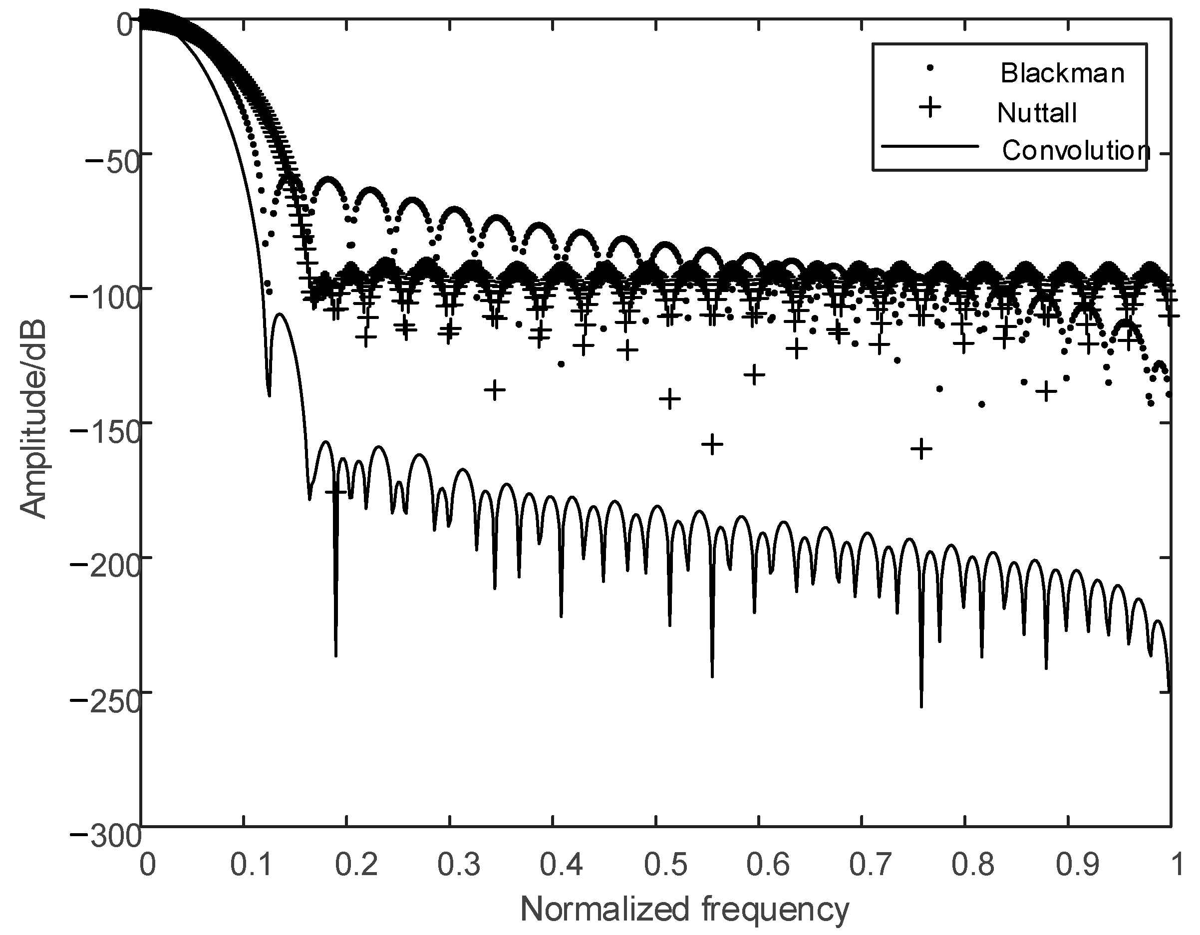
Table 1 presents the main and side lobe properties of five typical windows. It is concluded that the main lobe width of the Hamming and Hanning windows is relatively narrow, while the side lobe level is high and the attenuation rate is slow. The sidelobe levels of the Blackman–Harris and Nuttall windows are −92 dB and −83 dB, respectively, which are lower than the side lobe levels of the Hamming and Hanning windows. Although the Blackman–Harris and Nuttall windows have the advantages of low side lobe levels and high attenuation rates, their main lobe width is larger than that of the Hamming and Hanning windows. It can be seen that it is difficult for a single window to meet the requirements of a low main lobe width and high side lobe attenuation rate simultaneously.

To overcome the above contradictions, several scholars proposed compound convolution windows, which can be obtained via convolution operations using different single windows, such as the compound convolution window based on the Rife–Vincent window. According to the convolution theorem, the convolution of a signal in the time domain corresponds to the product on the frequency spectrum. Hence, the main lobe width of compound convolution windows is narrower than that of a typical single window, while the side lobe levels of compound convolution windows are much lower, and the side lobe attenuation rates are much higher than that of a single window.

To illustrate the advantages of compound convolution windows, the side lobe properties on the frequency spectrum of a compound convolution window, which is convolution of a Blackman window and a Nuttall window, are presented. The spectrum corresponding to Formula (1) is shown as follows.

$$W_B(\omega )={\displaystyle \sum _{i=0}^{M-1}\frac{{(-1)}^i{b}_i}{2}}\times [W_R(\omega -{\displaystyle \frac{2\pi i}{M}})+W_R(\omega +{\displaystyle \frac{2\pi i}{M}})]$$

(3)

where $W_R(\omega )$ is the frequency spectrum of the rectangular window, which is shown as follows.

$$W_R(\omega )={\displaystyle \frac{\sin \frac{\omega M}{2}}{\sin \frac{\omega }{2}}}{e}^{-j{\displaystyle \frac{\omega (M-1)}{2}}}$$

(4)

Let $\omega$ be $2\pi /N$; Formula (3) can be transformed into Formula (5), which is expressed as follows.

$$W_B({\displaystyle \frac{2\pi k}{N}})={\displaystyle \sum _{i=0}^{M-1}\frac{{(-1)}^i{b}_i}{2}}\times [W_R({\displaystyle \frac{2\pi k}{N}}-{\displaystyle \frac{2\pi i}{M}})+W_R({\displaystyle \frac{2\pi k}{N}}+{\displaystyle \frac{2\pi i}{M}})]$$

(5)

By substituting Equation (4) into Equation (5), the following expression is derived:

$$\begin{array}{l}{W}_B({\displaystyle \frac{2\pi k}{N}})=\sin ({\displaystyle \frac{\pi k}{2}})e{\displaystyle \frac{-jk\pi }{2}}{\displaystyle \sum _{i=0}^{M-1}\frac{{(-1)}^i{b}_i}{2}}\times \\ [{\displaystyle \frac{\sin (\frac{2\pi k}{N})+2j(1-{\sin }^2(\frac{2\pi k}{N})-\cos (\frac{\pi k}{N}))}{\sin [\pi (\frac{k}{N}-\frac{i}{M})]\sin [\pi (\frac{k}{N}+\frac{i}{M})]}}]\end{array}$$

(6)

Generally, N, the length of the signal, is much larger than 1, or N ≫ 1. Therefore, Formula (6) can be simplified as Formula (7), which is given as follows.

$$w({\displaystyle \frac{2\pi k}{N}})={\displaystyle \frac{N}{\pi }}\sin ({\displaystyle \frac{k\pi }{2}})e^{-j{\displaystyle \frac{\pi k}{2}}}\times {\displaystyle \sum _{i=0}^{M-1}{(-1)}^i\frac{b_i}{{\omega }^2-{(i)}^2}}$$

(7)

The number of cosine terms in the Blackman window is M = 3, with coefficients of 0.42, 0.5, and 0.08, respectively. The cosine coefficients of the Nuttall window are 0.3125, 0.46875, 0.1875, and 0.03125, respectively. Therefore, the formulae of the Blackman window and the Nuttall window are expressed as follows.

$$w_B(\omega )={\displaystyle \frac{N}{\pi }}\sin ({\displaystyle \frac{k\pi }{2}})e^{-j{\displaystyle \frac{\pi k}{2}}}\times ({\displaystyle \frac{0.42}{{\omega }^2}}-{\displaystyle \frac{0.5}{{\omega }^2-1}}+{\displaystyle \frac{0.08}{{\omega }^2-4}})$$

(8)

$$w_N(\omega )={\displaystyle \frac{N}{\pi }}\sin ({\displaystyle \frac{k\pi }{2}})e^{-j{\displaystyle \frac{\pi k}{2}}}\times ({\displaystyle \frac{0.3125}{{\omega }^2}}-{\displaystyle \frac{0.46875}{{\omega }^2-1}}+{\displaystyle \frac{0.1875}{{\omega }^2-4}}-{\displaystyle \frac{0.03125}{{\omega }^2-9}})$$

(9)

According to the convolution theorem, the frequency spectrum resulting from one convolution of the Blackman and Nuttall windows is equivalent to the product of Equations (8) and (9). This relationship is expressed by Formula (10) as follows.

$$w_{BN1}(\omega )=w_B(\omega )w_N(\omega )$$

(10)

The frequency spectra of the three formulas are shown in Figure 2.

Figure 2 shows that the peak side lobe of the compound convolution window is around −150 dB, which is lower than the −58 dB of the Blackman window and the −83 dB of the Nuttall window. It is clear that the side lobe attenuation rate of the convolution window is also much faster than that of the two windows. Therefore, the suppression effect of a compound convolution window on spectral leakage caused by incomplete periodic sampling is better than that of a single window.

If a two-fold convolution operation is applied to the Blackman window and the Nuttall window, the resulting spectrum is the square of Formula (10) as follows.

$$w_{BN2}(\omega )=w_B^2(\omega )w_N^2(\omega )$$

(11)

The spectra of Formulas (10) and (11) are shown in Figure 3.

As shown in Figure 3, the side lobe of the two-fold compound convolution window is better than that of the one compound convolution window, and the peak value of the side lobe of the two-fold compound convolution window is around −224 dB. Additionally, the side lobe attenuation rate is much higher. Similarly, the spectral characteristics of the triple compound convolution window are better than the two-fold compound convolution window. However, a two-fold compound convolution window is sufficient when the computational cost is taken into account. Considering all factors, the Blackman window and the Nuttall window are selected to compose the two-fold compound convolution window.

3. Spectral Line Interpolation

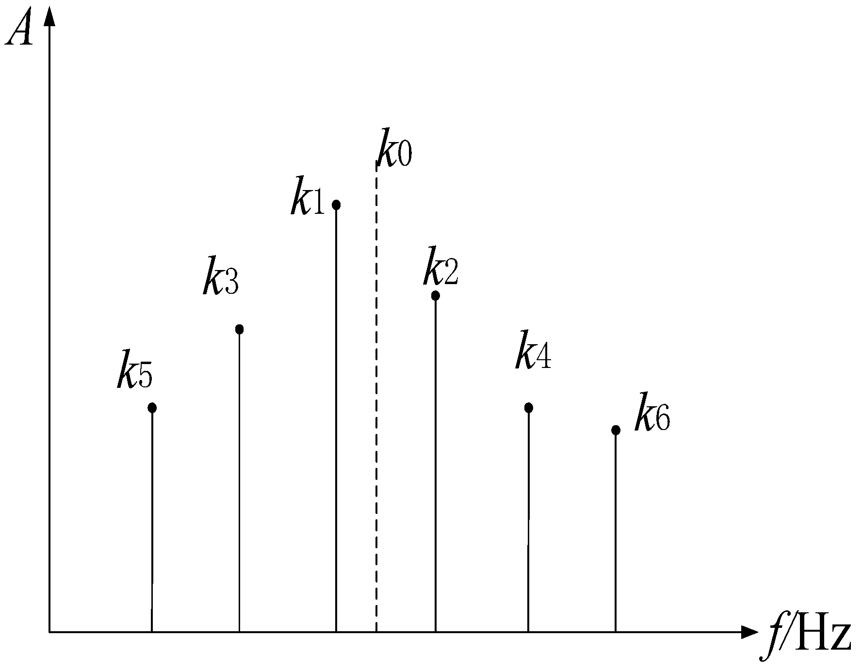
Due to frequency fluctuation and other factors, power line signals may experience incomplete periodic truncation. As a result, multiple spectral lines emerge near the true frequency points on the frequency axis rather than directly reflecting the true frequency values, as shown in Figure 4. Therefore, spectral line interpolation is required to accurately determine the true values of harmonic frequencies.

Generally, spectral line interpolation algorithms consist of three spectral lines, four spectral lines, six spectral lines, etc. The accuracy of the calculation improves as the number of selected spectral lines increases. Since harmonic analysis does not require high real-time performance, six spectral lines are employed for the interpolation algorithm to achieve higher precision results.

For simplifying the expression and excluding the influence of harmonics, the discrete formula of a sine wave signal is expressed as follows.

$$s(n)=A\sin (2\pi {\displaystyle \frac{f_0}{f_s}}n+\phi )$$

(12)

where A, $f_0$, and $\phi$ are amplitude, frequency, and initial phase, respectively. $f_s$ denotes the sampling rate, and n corresponds to the n-th sampling point. By multiplying this sinusoid signal, as given in Equation (12), with a two-fold compound convolution window, as described in Equation (11), the resulting equation is given by Equation (13).

$$x(n)=s(n)w_{BN2}(n)$$

(13)

and the corresponding spectrum is given in Equation (14), as follows.

$$X(\omega )={\displaystyle \frac{A}{2j}}[e^{j\phi }{W}_{BN2}(\omega -{\omega }_0)-e^{-j\phi }{W}_{BN2}(\omega +{\omega }_0)]$$

(14)

The formula above consists of two parts: the positive frequency part and the negative frequency part. In practice, only the positive frequency part is preserved, and the negative frequency part is omitted, so Formula (14) can be simplified to Formula (15).

$$X(\omega )={\displaystyle \frac{A}{2j}}{e}^{-j\phi }{W}_{BN2}(\omega -{\omega }_0)$$

(15)

The discretization form of Formula (15) is given as follows.

$$X({\displaystyle \frac{2\pi k}{N}})={\displaystyle \frac{A}{2j}}{e}^{-j\phi }{W}_{BN2}({\displaystyle \frac{2\pi (k-k_0)}{N}})$$

(16)

Given that the spectral line of the real frequency is $k_0$, we choose six spectral lines $k_1$–$k_6$, which are approximate to $k_0$, as depicted in Figure 4. The corresponding spectral line amplitude is $y_0$ = $\left|X({\displaystyle \frac{2\pi k_0}{N}})\right|$, $y_1$ = $\left|X({\displaystyle \frac{2\pi k_1}{N}})\right|$, $y_2$ = $\left|X({\displaystyle \frac{2\pi k_2}{N}})\right|$, $y_4$ = $\left|X({\displaystyle \frac{2\pi k_4}{N}})\right|$, $y_5$ = $\left|X({\displaystyle \frac{2\pi k_5}{N}})\right|$, and $y_6$ = $\left|X({\displaystyle \frac{2\pi k_6}{N}})\right|$. Let $\gamma$ = $k_0-k_1-0.5$ and $\gamma$ $\in$ [−0.5, 0.5]; we can obtain the following equations.

$$\begin{array}{l}{y}_1=\left|X({\displaystyle \frac{2\pi k_1}{N}})\right|\\ =\left|{\displaystyle \frac{A}{2j}}{e}^{-j\phi }{W}_{BN2}({\displaystyle \frac{2\pi (k_1-k_0)}{N}})\right|\\ =\left|{\displaystyle \frac{A}{2j}}{e}^{-j\phi }{W}_{BN2}({\displaystyle \frac{2\pi (-\gamma -0.5)}{N}})\right|\end{array}$$

(17)

Similarly, we can obtain the following equations.

$$y_2=\left|{\displaystyle \frac{A}{2j}}{e}^{-j\phi }{W}_{BN2}({\displaystyle \frac{2\pi (-\gamma +0.5)}{N}})\right|$$

(18)

$$y_3=\left|{\displaystyle \frac{A}{2j}}{e}^{-j\phi }{W}_{BN2}({\displaystyle \frac{2\pi (-\gamma -1.5)}{N}})\right|$$

(19)

$$y_4=\left|{\displaystyle \frac{A}{2j}}{e}^{-j\phi }{W}_{BN2}({\displaystyle \frac{2\pi (-\gamma +1.5)}{N}})\right|$$

(20)

$$y_5=\left|{\displaystyle \frac{A}{2j}}{e}^{-j\phi }{W}_{BN2}({\displaystyle \frac{2\pi (-\gamma -2.5)}{N}})\right|$$

(21)

$$y_6=\left|{\displaystyle \frac{A}{2j}}{e}^{-j\phi }{W}_{BN2}({\displaystyle \frac{2\pi (-\gamma +2.5)}{N}})\right|$$

(22)

Given that the spectral lines $k_1$ and $k_2$ are closer to the actual frequency $k_0$, while the other spectral lines are relatively distant, a larger weight value of 6 is assigned to $k_1$ and $k_2$, whereas the remaining weight values are 2, 2, 1, and 1, respectively. A new parameter $\beta$ is introduced, for which the expression is given as follows.

$$\beta ={\displaystyle \frac{(6y_2+2y_4+y_6)-(6y_1+2y_3+y_5)}{6y_2+2y_4+y_6+6y_1+2y_3+y_5}}$$

(23)

By substituting Equations (17)–(22) into Equation (23), we can obtain

$$\beta ={\displaystyle \frac{{\beta }_1}{{\beta }_2}}$$

(24)

where ${\beta }_1$ and ${\beta }_2$ are given as follows.

$$\begin{array}{l}{\beta }_1=6\left|W_{BN2}({\displaystyle \frac{2\pi (-\gamma +0.5)}{N}})\right|+2\left|W_{BN2}({\displaystyle \frac{2\pi (-\gamma +1.5)}{N}})\right|+\\ \left|W_{BN2}({\displaystyle \frac{2\pi (-\gamma +2.5)}{N}})\right|-6\left|W_{BN2}({\displaystyle \frac{2\pi (-\gamma -0.5)}{N}})\right|\\ -2\left|W_{BN2}({\displaystyle \frac{2\pi (-\gamma -1.5)}{N}})\right|-\left|W_{BN2}({\displaystyle \frac{2\pi (-\gamma -2.5)}{N}})\right|)\end{array}$$

(25)

$$\begin{array}{l}{\beta }_2=6\left|W_{BN2}({\displaystyle \frac{2\pi (-\gamma +0.5)}{N}})\right|+2\left|W_{BN2}({\displaystyle \frac{2\pi (-\gamma +1.5)}{N}})\right|+\\ \left|W_{BN2}({\displaystyle \frac{2\pi (-\gamma +2.5)}{N}})\right|+6\left|W_{BN2}({\displaystyle \frac{2\pi (-\gamma -0.5)}{N}})\right|+\\ 2\left|W_{BN2}({\displaystyle \frac{2\pi (-\gamma -1.5)}{N}})\right|+\left|W_{BN2}({\displaystyle \frac{2\pi (-\gamma -2.5)}{N}}\right|\end{array}$$

(26)

It can be seen that $\beta$ is a function of $\gamma$ from Equations (24)–(26). Due to the complexity of the equations, a polynomial is used to perform inverse fitting on this function, and we can obtain $\gamma$ = $f(\beta )$. It is sufficient to fit the highest term up to seven times in general. Consequently, the correction formula for frequency, initial phase, and amplitude are given as follows.

$$f_0=k_0\Delta f=(k_1+\gamma )f_s/N$$

(27)

$$\phi =\arg (X(k_1))-\pi \gamma$$

(28)

$$A={\displaystyle \frac{(6y_2+2y_4+y_6)-(6y_1+2y_3+y_5)}{{\beta }_2}}$$

(29)

To simplify the calculation of the aforementioned equation, the polynomial fitting method is employed, which leads to the introduction of a new mathematical function defined as follows.

$$h(\gamma )=N/{\beta }_2$$

(30)

Therefore, the correction formula for spectral amplitude is

$$A={\displaystyle \frac{(6y_2+2y_4+y_6-6y_1-2y_3-y_5)}{N}}h(\gamma )$$

(31)

where $h(\gamma )$ is

$$h(\gamma )=0.00162718+0.00021479{\gamma }^2+0.00001397{\gamma }^4+0.00000061{\gamma }^6$$

(32)

The aforementioned Formulas (27), (28), and (31) serve as fundamental computational formulas for signal parameter analysis. In scenarios involving signals composed of multiple harmonic components, it is essential to identify the maximum amplitude spectral line corresponding to each harmonic within the frequency spectrum.

4. Determination for Interference in Main Lobes

Insufficient frequency resolution may result in spectral main lobe interference caused by interharmonic components, leading to significant deviations in the calculated parameters of both harmonic and interharmonic components from their actual values. Therefore, it is necessary to study an effective methodology to identify main lobe interference phenomena.

Assuming that the DFT result of the signal in the power grid is $X_i(k)$, we process the spectrum by discarding the negative frequency components while preserving the positive frequency components, and the new spectrum is given as follows.

$$X_i(k)={\displaystyle \frac{A_i}{2j}}\exp (j{\phi }_i)W(k-k_i)$$

(33)

Suppose that $X_i(k_1)$ and $X_i(k_2)$ are two adjacent spectral lines within the main lobe of the i-th harmonic spectrum; Equations (34) and (35) can be obtained.

$$X_i(k_1)={\displaystyle \frac{A_i}{2j}}\exp (j{\phi }_i)W(k_1-k_i)$$

(34)

$$X_i(k_2)={\displaystyle \frac{A_i}{2j}}\exp (j{\phi }_i)W(k_2-k_i)$$

(35)

Given that k₂ = k₁ + 1, substituting k₂ = k₁ + 1 into (35) yields Equation (36) as follows.

$$\begin{array}{l}{X}_i(k_1+1)={\displaystyle \frac{A_i}{2j}}\exp (j{\phi }_i)W(k_1+1-k_i)\\ ={\displaystyle \frac{A_i}{2j}}\exp (j[{\phi }_i-(k_1+1-k_i)\pi ])W(k_1+1-k_i)\end{array}$$

(36)

Hence, the absolute value of the phase difference between $X_i(k_1)$ and $X_i(k_2)$ is

$$\left|\Delta {\phi }_i\right|=\left|[{\phi }_i-(k_1+1-k_i)\pi ]\right.-\left.[{\phi }_i-(k_1-k_i)\pi ]\right|=\pi$$

(37)

Based on Equation (37), in the absence of spectral lines interference within the main lobe, the absolute value of the phase difference between two adjacent spectral lines on the spectrum is $\pi$ radians, which is equivalent to 180° degrees. In contrast, the absolute value of the phase difference between adjacent spectral lines deviates from 180°. Given the presence of unfavorable factors such as signal noise and calculation errors, the following formula is utilized to identify the main lobe interference.

$$\Delta {\phi }_i=\left|\arg (X_i(k))-\arg (X_i(k+1)))-{180}^{\circ }\right|>\epsilon$$

(38)

where $\arg (X_i(k))$ denotes the phase of the spectral line $X_i(k)$, i is the i-th harmonic component, and $\epsilon$ is the threshold of $\Delta {\phi }_i$ in Equation (38); here, the units of $\epsilon$ are in degrees. From a theoretical perspective, $\Delta {\phi }_i$ should ideally be 0° in the absence of interference within the main lobe. However, practical considerations, such as system noise and computational inaccuracies, typically result in a slight deviation, yielding $\Delta {\phi }_i$ marginally greater than 0°. Based on empirical observations and theoretical analysis, we establish a conservative threshold of $\epsilon$ = 5° for reliable interference detection. The phase difference caused by noise and errors is small, and the phase difference when main lobe interference occurs is high, so this 5° threshold can ensure the accurate identification of main lobe interference.

5. ZoomFFT

In power system scenarios, the frequency spacing between harmonics and interharmonics may be narrow, potentially inducing spectral aliasing phenomena during the harmonic analysis of power signals. This significantly compromises the accuracy of harmonic parameter estimation. To address this limitation, ZoomFFT is utilized to effectively suppress spectral aliasing while facilitating the calculation of harmonic parameters. The procedures of ZoomFFT are comprehensively presented as follows.

(1): Firstly, the presence of main lobe interference can be identified by Equation (38). In cases where main lobe interference is detected, it is necessary to ascertain the specific frequency band that is affected. Subsequently, the lowest frequency ${\omega }_l$, the central frequency ${\omega }_0$, and the highest frequency ${\omega }_h$ can be determined. By multiplying the signal x(t) of length N with the rotation factor $e^{-j{\omega }_{0}t}$, the frequency spectrum of the signal is shifted to zero frequency, yielding a new spectrum $X^{\prime }(\omega )$.

(2): A low-pass filter is applied to the new spectrum $X^{\prime }(\omega )$, retaining the low-frequency part of $X^{\prime }(\omega )$ and eliminating the high-frequency part.

(3): The inverse fast Fourier transform (IFFT) is applied to the low-pass filtered data with N points, obtaining a time domain signal $x^{\prime }(t)$. Then, down sampling is carried out at intervals of D, producing a new signal of length N/D.

(4): FFT is applied to the signal $x^{\prime }(t)$ of length N/D, which is then rearranged. By setting the number of Fourier transform points to N, a frequency spectrum of length N is generated. The original frequency interval $\Delta \omega$, or ${\omega }_h$ − ${\omega }_l$, is divided by D, resulting in a new frequency interval $\Delta \omega /D$. Therefore, the frequency resolution increases by D times, achieving the objective of the local amplification of the spectrum.

In summary, a flowchart of the algorithm in this article is shown in Figure 5.

6. Experimental Results and Analysis

To validate the effectiveness of the algorithm proposed in this study, voltage signals containing harmonics and interharmonics were analyzed. The amplitude, frequency, and phase parameters derived from the analysis are given in

Table 2. Analog signal amplitude, frequency, and initial phase.

Signal Components	Amplitude/V	Frequency/Hz	Initial Phase/(°)
1	5	30	15
2	220	50	45
3	10	52	50
4	7	55	80
5	10	100	150
6	5	150	100
7	6	200	30
8	5	250	90

.

The frequency of harmonics exceeds 2.5 kHz. According to the Nyquist theorem, the sampling frequency must be greater than 5 kHz. In this study, it was set to 6400 Hz. Furthermore, the sampling length was 10 cycles, which is equivalent to 1280 sampling points. The amplification factor D in ZoomFFT was chosen as 10.

To account for noise interference in real-life signals, Gaussian white noise with a signal-to-noise ratio of 50 dB was added to the signal to simulate the real noise. The harmonics and interharmonics of the signal were analyzed by using the algorithm proposed in this article, and the results are detailed in

Table 3. The simulation results by the proposed algorithm.

Signal Components	Amplitude/V	Frequency/Hz	Initial Phase/(°)
1	5.0037	29.9989	15.3326
2	219.9907	50.0000	45.0223
3	10.0508	51.9983	51.5665
4	7.0439	55.0001	80.3867
5	9.9944	99.9989	149.9650
6	5.0057	149.9964	100.3381
7	5.9898	199.9979	30.0387
8	5.0131	249.9993	90.9629

.

As shown in Table 2, the proposed algorithm effectively calculates the parameters of harmonics and interharmonics even under a signal-to-noise ratio of 50 dB. The relative errors of the amplitude, frequency, and initial phase of each harmonic were then determined by Equations (39) to (41) as follows.

$$\Delta A={\displaystyle \frac{\left|A(i)-A^{\prime }(i)\right|}{A(i)}}\times 100\%$$

(39)

$$\Delta f={\displaystyle \frac{\left|f(i)-f^{\prime }(i)\right|}{f(i)}}\times 100\%$$

(40)

$$\Delta \phi ={\displaystyle \frac{\left|\phi (i)-{\phi }^{\prime }(i)\right|}{\phi (i)}}\times 100\%$$

(41)

where $A(i)$, $f(i)$, and $\phi (i)$ represent the real parameter of the i-th harmonic or interharmonic and $A^{\prime }(i)$, $f^{\prime }(i)$, and ${\phi }^{\prime }(i)$ are the calculation result of the i-th harmonic or interharmonic. The relative errors of the parameters for each harmonic are illustrated in Figure 6, Figure 7 and Figure 8.

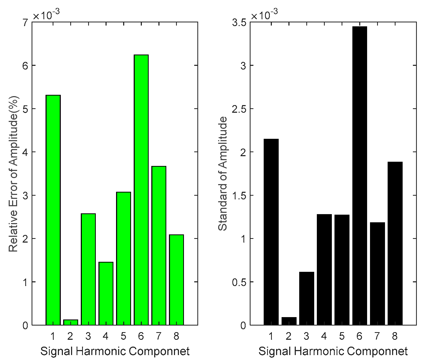
As illustrated in Figure 6, Figure 7 and Figure 8, the relative errors between the calculated values and actual values of each harmonic and interharmonic parameter remain relatively minimal. Specifically, the relative errors of amplitude do not exceed 9 × 10⁻³%, while the errors of frequency are within 5 × 10⁻⁵%. Although the initial phase exhibits a comparatively larger error, it remains below 4 × 10⁻²%, which is still considered negligible.

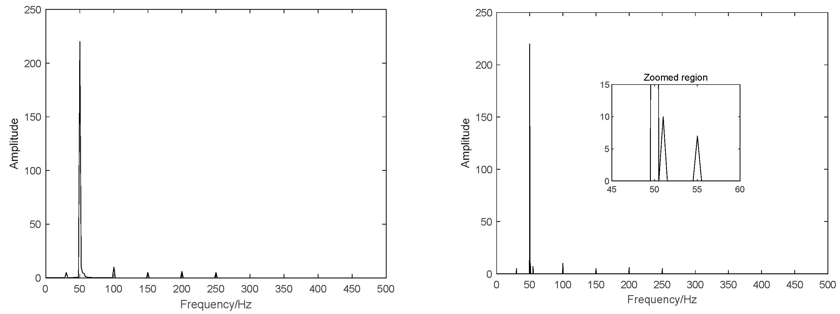
Additionally, Figure 9 shows the different harmonic analysis results. The left picture shows the results of traditional FFT, which failed to identify the approximate frequencies.

In contrast, the right picture demonstrates that the proposed method can identify the approximate frequencies successfully, which proves the effectiveness of the method.

Furthermore, to validate the stability of the algorithm, five Monte Carlo experiments were conducted. The results demonstrate that the standard of amplitude is less than 0.04, the standard of frequency is less than 3.5 × 10⁻³ Hz, and the standard of initial phase is less than 1.5°. The findings indicate that the standards of the computation results are small enough, thereby confirming the reliability of the algorithm.

To verify the superiority of the proposed algorithm over the competing algorithms, a comparative analysis was conducted by using the Blackman window, the Hanning window, the Hamming window, ZoomFFT, and the proposed algorithm. Each algorithm was executed 10 times in Monte Carlo simulations to evaluate the computational time required for each run. The average of the 10 execution times was calculated and used as the representative time cost for a single run. The results are shown in

Table 4. Comparison of algorithm running results and duration.

Algorithms	Resolution	Sampling Points	Running Time/ms
Blackman	incomplete	1280	7.31
Hanning	incomplete	1280	7.35
Hamming	incomplete	1280	7.30
ZoomFFT	complete	12,800	51.65
Proposed	complete	1280	12.41

.

The statistics in Table 3 demonstrate that the three windowed interpolation methods were unable to identify interharmonics and resulted in incorrect calculation results. Although ZoomFFT can successfully identify interharmonics, it demands a large number of sampling points and prolonged computation time, as it lacks a main lobe interference detection step and requires frequency axis amplification for each component. The proposed algorithm, which incorporates main lobe judgment and ZoomFFT, can precisely distinguish main lobe interference and calculate the parameters of both harmonics and interharmonics.

7. Conclusions

A combined algorithm integrating a compound convolution window and ZoomFFT was designed to achieve accurate measurement of harmonic and interhamonic parameters. This algorithm leverages the benefits of a two-fold compound convolution window, including the low side lobe peak and high attenuation rate, to effectively mitigate spectral leakage and aliasing. Furthermore, by incorporating the high-frequency resolution capability of ZoomFFT, the algorithm addresses the issue of inaccurate calculations caused by interference from adjacent interharmonics, ensuring enhanced accuracy in parameter estimation. The analysis results of simulated signals verified that the algorithm has the merits of high estimation accuracy and low time cost, providing an outstanding alternative for harmonic control in modern power grids. In the future, there is a need for further exploration into the development of an FPGA-based device, the integration of the proposed algorithm onto this device, and its practical application in the harmonic detection of real-life power grids.