Article

Proposal of a Thermal Network Model for Fast Solution of Temperature Rise Characteristics of Aircraft Wire Harnesses

by
Tao Cao
1,
Wei Li
2,
Tianxu Zhao
2,* and
Shumei Cui
2
1
Shanghai Aircraft Design and Research Institute, Commercial Aircraft Corporation of China, Shanghai 201210, China
2
School of Electrical Engineering and Automation, Harbin Institute of Technology, Harbin 150001, China
*
Author to whom correspondence should be addressed.
Energies 2025, 18(15), 4046; https://doi.org/10.3390/en18154046
Submission received: 23 June 2025 / Revised: 18 July 2025 / Accepted: 24 July 2025 / Published: 30 July 2025
(This article belongs to the Section F: Electrical Engineering)

Abstract

The design of aircraft electrical wiring interconnection systems (EWISs) is central to ensuring the safe and reliable operation of aircraft. The calculation of the temperature rise characteristics of aircraft wire harnesses is one of the key technologies in EWIS design, directly affecting the safety margin of the system. However, existing calculation methods generally face a bottleneck in the balance between speed and accuracy, failing to meet the requirements of actual engineering applications. In this paper, we conduct an in-depth study on this issue. Firstly, a finite element harness model is established to accurately obtain the convective heat transfer coefficients of wires and harnesses. Based on the analysis of the influencing factors of the thermal network model for a single wire, an improved thermal resistance hierarchical wire thermal network model is proposed. A structure consisting of series thermal resistance within layers and iterative parallel algorithms between layers is proposed to equivalently integrate and iteratively calculate the mutual thermal influence relationship between each layer of the harness, thereby constructing a hierarchical harness thermal network model. This model successfully achieves a significant improvement in calculation speed while effectively ensuring useable temperature rise results, providing an effective method for EWIS design.

1. Introduction

An electrical wiring interconnection system (EWIS) is an integrated system of all the electrical wiring in an aircraft, including wires, wire harnesses, connectors, and related support components. Among these, a wire harness is the result of bundling multiple wires together with binding straps or sleeves. The temperature rise design capability of aircraft wires and harnesses is a core indicator of the quality of the design of an electrical wiring interconnection system (EWIS) for aircraft design units, and it is also a key technical support for the development of advanced aircraft with multi-electrification, integration, and high reliability [1]. In EWIS design, the wire temperature rise directly determines the safety margin of the system—an excessive rise in temperature may lead to insulation aging, short circuits, or even fires [2,3,4]. Therefore, calculation methods that balance time-efficient engineering and physical accuracy are urgently needed.
Existing methods for calculating the temperature rise in wires and harnesses include analytical methods and finite element simulation methods. Analytical calculation methods [5,6,7] quickly estimate the average/maximum temperature rise based on simplified formulas, using the fastest calculation speed. However, the derivation of formulas requires a large amount of data fitting, and has disadvantages such as an inability to reflect the axial temperature difference in wire harnesses, weak dynamic analysis capability, and high accuracy only within specific ranges, making it difficult to perform temperature rise calculation for complex aircraft harnesses. The current-carrying capacity method [8,9,10,11] relies on IEC standard empirical formulas; however, it has difficulties in convergence when harnesses are coupled, and its formula verification is time-consuming. The value of its current-carrying capacity needs to be constantly corrected, and it is necessary to constantly check whether each wire exceeds the allowable working temperature [12]. There are no specific empirical formulas for aircraft harnesses. Traditional thermal network methods [13,14,15,16,17,18,19] have a low dependence on empirical parameters and can analyze temperature differences in the axial direction of wires, but they also have shortcomings, such as the calculation accuracy being related to the number of nodes analyzed, the inability to analyze complex harnesses, and unsuitability for analyzing dynamic temperature rise. Although simple to model and efficient in calculation, the solution accuracy highly depends on how accurate the thermal resistance topology model is. The finite element method is mainly classified into two types based on its complexity as follows: finite element analysis, considering only electrothermal coupling; and finite element analysis, considering both electrothermal and fluid–thermal coupling. Electrothermal coupling takes into account the interaction between the electric field and the thermal field. By simultaneously solving the current field (Ohm’s law) and the heat conduction equation, the influence of the Joule heat generated by the current on temperature rise can be accurately reflected. This is a common approach in finite element analysis of existing wire harnesses [20,21]. In more complex wire harness application scenarios, fluid–thermal coupling needs to be considered to expand the electrothermal coupling finite element analysis. This analysis method not only calculates the Joule heat generated by the electric field and the resulting changes in the temperature field, but also the influence of the fluid field [22,23,24]. It achieves high-precision simulation through 3D solid modeling, analyzing the dynamic temperature rise in wire harnesses and exhibiting a better performance in detecting the axial temperature difference in harnesses compared to the thermal network method. However, for complex aircraft harnesses, the calculation accuracy of the model is closely related to the accuracy of the physical model and the density of the mesh division. High-precision models can be used to describe the temperature rise in the conductor, but they occupies more resources and take longer to calculate; this still requires further optimization.
To investigate the contradiction among speed, accuracy, and complexity, this paper proposes an iterative thermal network calculation model of “series within layers and parallel between layers”. The main contributions of this paper are as follows:
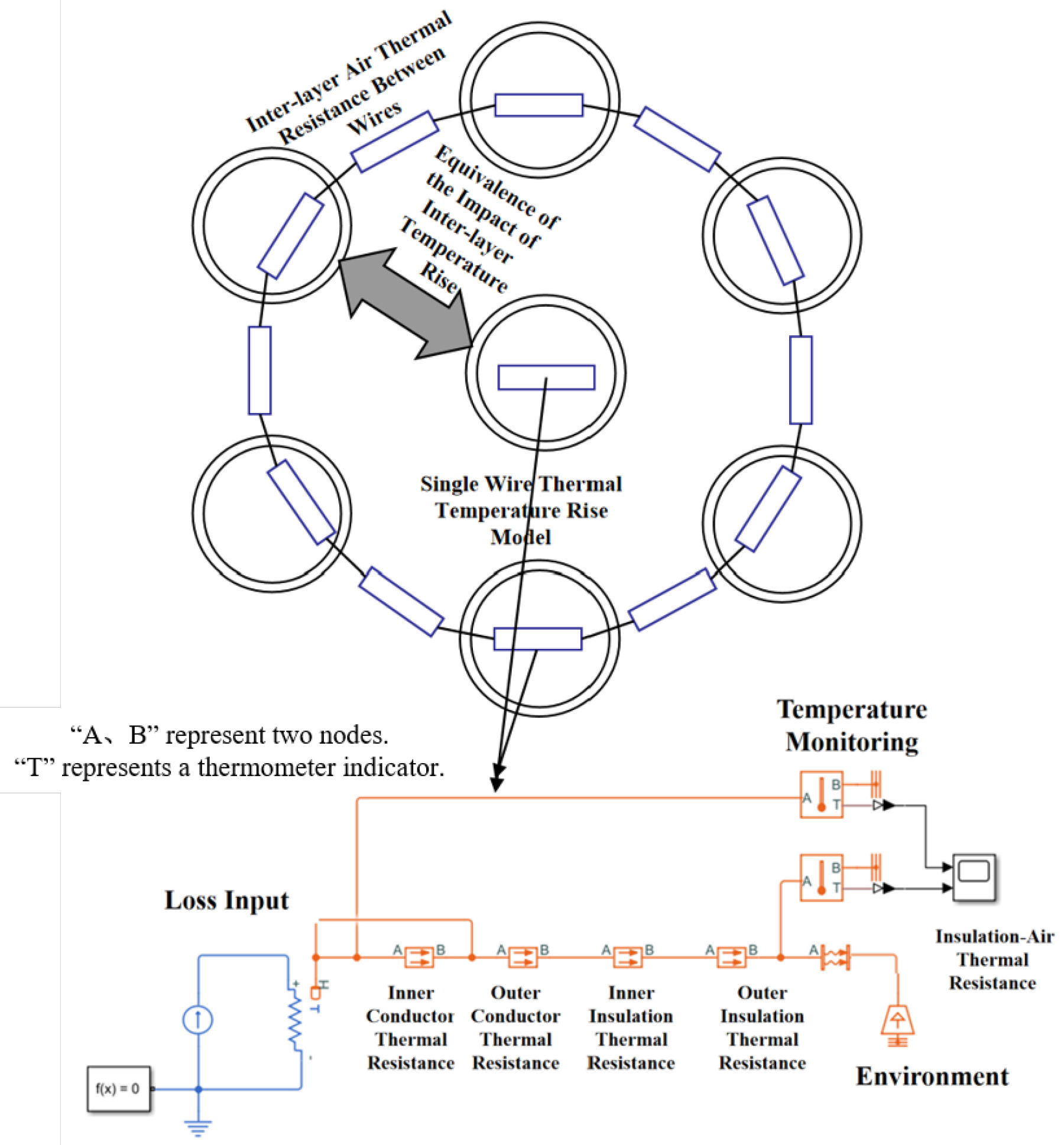
  • Establishment of a reasonable precision thermal resistance hierarchical wire thermal network, in which the wire core conductor and insulation layer are divided into inner and outer layers. The model accuracy is corrected through the thermal resistance of the inner and outer layers [25]. Meanwhile, thermal resistance is added between the outer layer of the insulation and the external ambient air to simulate the heat dissipation loss caused by changes in the material properties, thereby improving the model accuracy.
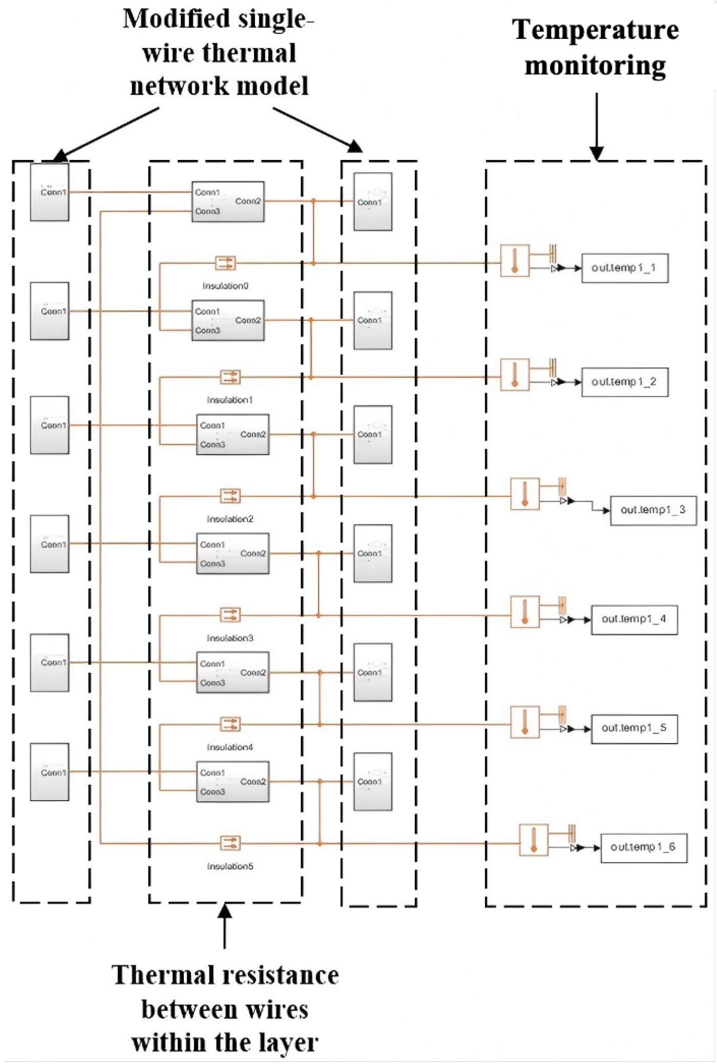
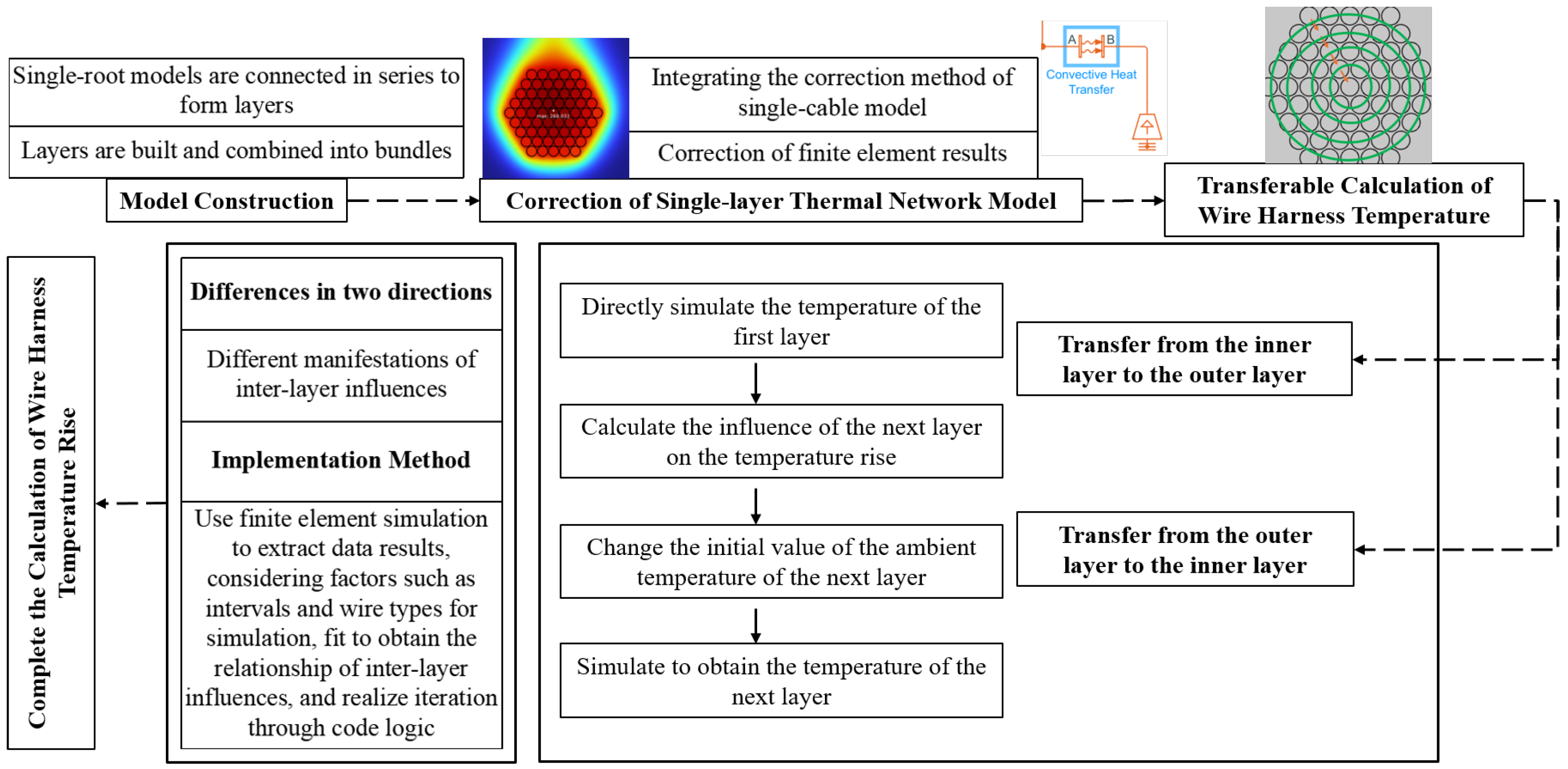
  • Construction of a hierarchical harness thermal network model based on finite element model correction—through the topology of the thermal resistance hierarchical wire thermal network, a structure of “series within layers and parallel between layers” is constructed. By conducting power-on simulations on the finite element single-layer model, the convective heat transfer coefficients of each layer’s thermal network model are improved to construct the hierarchical harness thermal network model.
  • Hierarchical thermal network iterative calculation method—based on the hierarchical harness thermal network model, the interlayer influence is equivalently constructed through the finite element model results, and the rapid calculation of the hierarchical thermal network model is achieved through the interlayer model iterative algorithm.
The structure of the paper is as follows: first, the process of establishing the high-fidelity finite element model is introduced; then, the influencing factors of the wire thermal network model are analyzed and the thermal resistance hierarchical wire thermal network model is constructed. The wire thermal network model is expanded to obtain the hierarchical harness thermal network model, and finally, fast calculation of the latter is realized through the iterative algorithm.

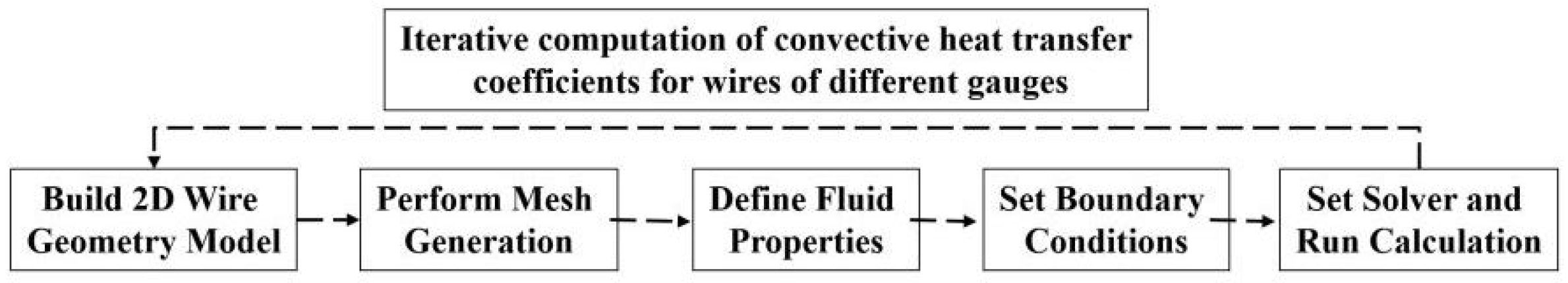
2. Construction of a High-Fidelity Finite Element Model and Determination of the Convective Heat Transfer Coefficient

The convective heat transfer coefficient h is affected by factors such as the geometric shape of the object, fluid properties (viscosity and density), flow state (laminar or turbulent flow), and flow mode (forced or natural convection), making it difficult accurately calculate it using analytical methods. This coefficient can be obtained through the fluid simulation function of the finite element method, thereby simplifying a large number of complex calculations. The specific process is shown in Figure 1. The convective heat transfer coefficients of different gauge wires are solved through repeated cycles to obtain the relationship curve between the wire gauge and the convective heat transfer coefficient. Finally, the curve values of the convective heat transfer coefficient are substituted into the analytical formula.
When establishing the model through the finite element method, the following aspects need to be noted:
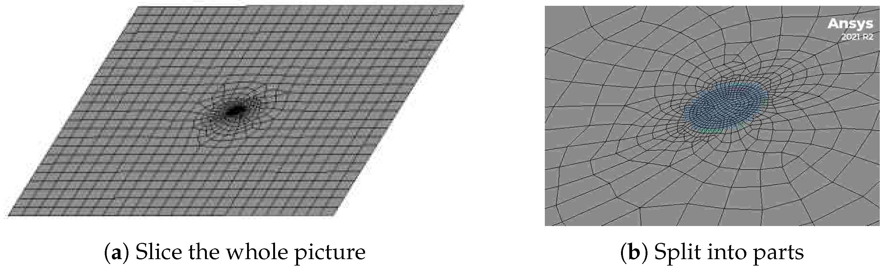
  • Modeling and grid generation: create the fluid domain and solid surface, and then use the meshing tool to discretize the geometric model to generate a computational grid suitable for calculating fluid flow and heat transfer. The meshing quality is crucial to the calculation results, directly affecting the calculation accuracy of wire temperature rise. Especially in the boundary layer area, sufficiently fine grids are required to capture the temperature gradient and velocity gradient of the fluid. The finite element grid is shown in Figure 2.
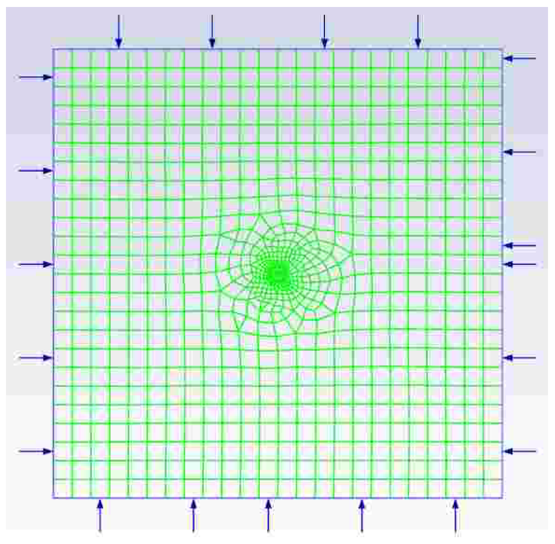
  • Setting the boundary conditions of the model: select a suitable laminar flow model or turbulent flow model according to the specific application scenario, and set the inlet boundary conditions and outlet boundary conditions, such as the fixed pressure, flow rate, and ambient temperature. The grid diagram after setting the model boundary conditions is shown in Figure 3.
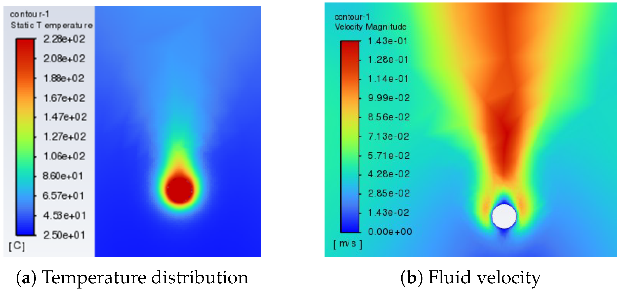
  • Setting the solver and calculating: select an appropriate solver and numerical method, and set appropriate convergence criteria for iterative control. The convergence of the calculation process is judged by monitoring the changes in physical quantities (such as flow rate, temperature and residual). After the calculation is completed, check the temperature distribution, velocity field, and heat flux density of the flow field to ensure that the results meet the physical expectations.
In this study, the wires are placed horizontally, and there is no axial temperature gradient in natural convection. Therefore, a two-dimensional simplification is supported. The physical basis is that the direction of gravity is perpendicular to the length of the wire, and the lifting force only acts on the cross-section, similar to the problem of flow around a cylinder. The heat dissipation mode of the wire is natural convection. The flow state of natural convection can be determined by the Grashof number ( G r ) and the Prandtl number ( P r ). When G r P r 10 9 , the fluid is laminar; otherwise, it is turbulent. G r is positively correlated with the temperature difference and characteristic length, while the P r mainly depends on the type of fluid. For air, P r varies with temperature, but has little impact and is usually taken as 0.7. In this study, the ambient temperature is 25 °C, and the temperature range is limited to 260 °C, which is chosen according to the system requirements to avoid damage caused by excessively high temperatures. Both the calculation and the experiment adhere to this limit. The calculated G r P r is approximately 1.2 × 10 4 , confirming laminar natural convection. The surface roughness of the wire was not tested in this study. According to industry standards, it is assumed to be 1.6 μm, in line with the ISO 1302 [26] processing standard, with a “commercially polished” surface finish, corresponding to an emissivity of 0.8.
The air thermal conductivity under normal pressure is fixed, and the convective heat transfer coefficient should decrease with the increase in the wire diameter. The fluid model is used for simulation, then fitted and substituted into the wire thermal balance formula to reduce the calculation amount while ensuring the calculation accuracy. In the finite element model, only convective heat dissipation, and no radiation heat dissipation, is set. The four surrounding boundaries are set as open boundaries; that is, gas is allowed to flow freely in and out to simulate an infinite space. The simulation results of an AWG10 wire under a 101 A [27] current at normal temperature and pressure are shown in Figure 4, where Figure 4a is the temperature distribution and Figure 4b is the flow velocity distribution.
In order to obtain the convective heat transfer coefficients of different wires at different temperatures and altitudes, the relationship between temperature, pressure, and altitude is first established [28], as shown in Figure 5. To determine the relationship between pressure and the convective heat transfer coefficient, it is necessary to first use fluid finite element software to simulate the convective heat transfer coefficient under different pressures. Ambient pressures of 18 kPa, 40 kPa, 60 kPa, 80 kPa, and 101.4 kPa are selected to determine the convective heat transfer coefficients of single wires with different wire gauges, and the results are shown in Figure 6. At a normal pressure of 101 kPa, the air convection heat dissipation effect is good, and the corresponding convective heat transfer coefficient is the largest. As the air pressure decreases, the convective heat transfer coefficient gradually decreases. The data are interpolated to obtain the relationship between the convective heat transfer coefficient and the wire diameter at any pressure, as shown in Figure 2, Figure 3, Figure 4, Figure 5, Figure 6 and Figure 7. From Figure 7, the curves of the variation in convective heat transfer coefficient with the wire diameter at pressures of 75.35 kPa and 19.75 kPa are obtained, as shown in Figure 8.
Under the assumption that the arrangement of the harness is known (wire harnesses on aircraft are mainly arranged in a near-circular shape), a typical harness is selected, and a finite element model is utilized to solve the convective heat transfer system. Take a harness composed of 19 wires as an example, as shown in Figure 9. In actual wiring harnesses, slight deformation of the wires (such as compression of the insulation layer or an imperfect circular arrangement) can form microscopic air gaps (about 0.1–0.3 mm), which is inevitable and a key contributing factor to heat dissipation issues in wiring harnesses. This must be taken into account. However, the complexity of the problem lies in the fact that the tiny air gaps formed by different wires are uncontrollably different from each other. In some cases, the adjacent wires do not come into direct contact, but have an air gap between them. In other cases, due to the squeezing effect, the adjacent wires are in direct contact, with only a small triangular air space left at the non-covered position of the circular cross-section. In the calculation, we disregarded the aforementioned complex factors and assumed that the air gap of each layer was equal for convenience. Figure 9 is only a schematic diagram; the intervals between the wires in this diagram are exaggerated and do not represent the actual situation.
In harness modeling, the constraints that need to be considered are as follows:
  • Envelope size limit: according to the installation space requirements, the outer diameter of the wire harness must be kept within a certain range.
  • Bending radius limit: the minimum bending radius should be greater than or equal to five times the diameter of the wire harness to prevent excessive squeezing and mechanical damage.
For series thermal network models constructed in layers, the network model of each layer requires the input of its corresponding convective heat transfer coefficient. In this paper, a complete finite element model of a wiring harness is established, comprehensively considering factors that have a significant impact on the convective heat transfer coefficient, such as line type, altitude, and wire gap. By assigning current values to the single-layer wire harnesses in the finite element model separately and modifying the equivalent convective heat transfer coefficients corresponding to the hierarchical thermal network model, the temperature rise results of the two are consistent; thus, the convective heat transfer coefficients could be corrected. Meanwhile, by changing influencing factors such as the line type, multiple sets of simulations are conducted to determine the relationship between the convective heat transfer coefficient of each layer of the series heat network model and the above-mentioned influencing factors, thereby achieving rapid calculation of the intra-layer heat transfer in the single-layer heat network model.
The geometric model of the wire harness is established based on the size constraints of its external wiring and the type and quantity constraints of its conductors. When converting from the geometric model to the finite element model, the conductors and insulation layers of the wires conduct heat in a solid state and can easily reach equilibrium. The methods for setting its thermal power and heat transfer coefficient are the same as those for a single wire. The air domain wrapping the wire harness is discretized into independent concentric layers, matching the number of wire harness layers according to the thermal gradient characteristics. By radially partitioning the air domain, the evolution of the thermal boundary layer can be accurately described, avoiding the distortion of the heat dissipation path caused by the assumption of overall homogenization, thereby improving the calculation accuracy. Subsequently, by assigning current values to each single layer of the wire harness in the finite element model, the equivalent convective heat transfer coefficient of the corresponding hierarchical thermal network model is modified at the same time to keep the temperature rise results of the two consistent, correcting the convective heat transfer coefficient in the hierarchical thermal network model. Meanwhile, multiple sets of simulations are conducted by changing the line type to obtain the convective heat transfer of each layer of the series thermal network model. The corresponding results are shown in Figure 10.

3. Construction of Thermal Resistance Hierarchical Aircraft Wire Thermal Network Mode

To reduce the complexity of the thermal network model, the following assumptions and simplifications are made for the thermal network model:
  • Both the wire and the insulation layer are regarded as uniform and isotropic materials.
  • The interfacial thermal resistance between layers (such as the interface between conductors and insulators) is simplified to a concentrated thermal resistance, and local non-uniformity is ignored.
  • The temperature distribution at each thermal network node (such as the conductor core and insulation layer) is assumed to be uniform, and the internal gradient is ignored.
  • In the steady-state simulation, the convective heat transfer coefficient is set at a constant level, and its variation with the increase in temperature is ignored.
  • Since its contribution to the total heat dissipation under operating conditions is less than 5%, radiative heat transfer is ignored.
Figure 11 shows the traditional wire thermal network model built in MATLAB r2022a Simulink, which consists of loss input, core conductor thermal resistance, insulation layer thermal resistance, and the external environment. For calculation convenience, the thermal loss of the wire and the thermal resistance of the conductor and insulation layer are all calculated with a unit length of 1 m. At the same time, the temperature rise is recorded during model construction. For a single wire, the traditional thermal network model idealizes the wire conductor as a solid conductor; thus, this model is relatively simple and the calculation errors are large.
Analyzing the differences between the thermal network and finite elements, the sources of error in thermal network simulations may include the following:
  • An uneven distribution of the wire core and insulation layer. The material properties in the finite element will automatically change with temperature, but the thermal network model cannot consider this change, so the relative error is high. Considering that the wire loss is generated in a three-dimensional body, and heat dissipation ultimately depends on the outer surface of the insulation layer, the larger the diameter, the worse the heat dissipation conditions of the wire and the more uniform the temperature distribution in the wire. Therefore, the larger the diameter, the smaller the error in the thermal network.
  • Changes in thermal resistance at the interface between the core and the insulation layer and between the insulation layer and the air layer, as well as a change in materials, which will cause a certain reduction in the wire’s heat dissipation effect. The wire is actually composed of individual cores, and is not a single solid. There are also air gaps between the cores. The traditional thermal network model simplifies the wire conductor into a solid conductor. If each wire core is to be modeled, the thermal network model becomes very complex; therefore, a new model simplification method needs to be created to ensure the accuracy of the calculation results and simplify the model as much as possible. For this reason, in this paper, we create a thermal resistance hierarchical simplified thermal network method for the establishment and calculation of thermal network models.
Based on the simple model construction of a single wire, multiple cores are simplified into a solid conductor. If a refined wire model is to be established to construct a thermal network model, the thermal network model will be very complex. In order to ensure the calculation accuracy of the thermal network model without making the model too complex, this paper divides the wire core conductor and insulation layer into inner and outer layers. The model accuracy is corrected through the thermal resistance of the inner and outer layers. At the same time, thermal resistance is added between the outer layer of the insulation and the external ambient air to simulate the heat dissipation loss due to changes in the material properties of the insulation and air, so as to correct the model accuracy, as shown in Figure 12.
In order to correct the above two factors, a thermal resistance hierarchical thermal network calculation model for a single wire is established, as shown in Figure 13.
Compared with the traditional thermal network model, the thermal resistance hierarchical thermal network model has made the following improvements and optimizations:
  • To take into account the temperature differences at different positions of the wire, in the modeling of the thermal resistance of the wire layering, the copper core and the insulating layer are, respectively, divided into inner and outer layers. Among them, copper is used as the thermal conductor, and an insulator is used for the insulating layer. This layering treatment divides the geometric boundary through the median diameter. Compared with the air environment, the two are presented as a whole, where the inner layer temperature is relatively higher, and the thermal resistance is specifically increased.
  • Thermal resistance is added between the outer layer of the insulation and the external ambient air to simulate the heat dissipation loss caused by changes in the material properties of the insulation and air. At the same time, to simulate the heat dissipation loss due to changes in the material properties of the conductor and insulation layer, the thermal resistance of the outer conductor and inner insulation layer is correspondingly increased.
  • During the analysis process, based on the theoretical thermal resistance calculation values of the conductor’s layered structure and in combination with the temperature distribution characteristics observed in actual tests, we empirically adjusted the thermal resistance parameters of each region of the conductor and insulation layer. By comparing the thermal performance data under different line types and working conditions, the correction range for increasing the thermal resistance of the inner conductor by 6.5~8.5% and that of the outer conductor and inner insulation layer by 3.5~4.5% was determined. This correction scheme can better reflect the actual heat transfer characteristics and ensure the applicability of the model to different types of conductors.
Three sets of linear temperature rise tests were conducted, and the results are shown in Table 1. By verifying that the current passed through the experimental, improved wire thermal network model and that the error of the finite element model at 260 ℃ was within the error of the ratio of the difference between the simulated current and the actual current to the actual current, it was verified that the error of the wire thermal network with stratified thermal resistance was less than 6%. A hierarchical thermal network model can be formed by series connections.

4. Aircraft Harness Thermal Network Model

4.1. Construction of a Hierarchical Harness Thermal Network Model

Based on the thermal resistance hierarchical single-wire thermal network model presented in Section 3, a hierarchical harness thermal network model is constructed. To build a layered thermal network model with series connections within layers and parallel connections between layers, the multi-layer wire harnesses are first decomposed into axial layers, and the complex heat transfer of the wire harness is decomposed into two parts as follows: heat transfer within layers, and heat transfer between layers. For the heat transfer within layers, the previously mentioned wire thermal network model is connected in series with air thermal resistance, which is called series connection within layers. This is used to simulate the heat transfer within the layer, while the heat transfer between layers is equivalent to the change in the value of the ambient temperature in the model. The temperature rise in the multi-layer wiring harness is calculated through a recursive method.
Taking seven wires as an example, Figure 14 shows the central wire and the first-layer architecture of the harness thermal network model. The thermal resistance hierarchical wire thermal network model of a single wire is packaged and combined. Each wire is modeled using the thermal resistance hierarchical wire thermal network model, and the air thermal resistance between the wires within the layer is supplemented into the wires within the layer to form the first-layer harness thermal network model, as shown in Figure 15. The second, third and fourth layers are established in sequence, as shown in Figure 16.

4.2. Interlayer Transferable Fast Calculation Method

The idea of interlayer transfer calculation is shown in Figure 17, and the detailed steps are as follows:
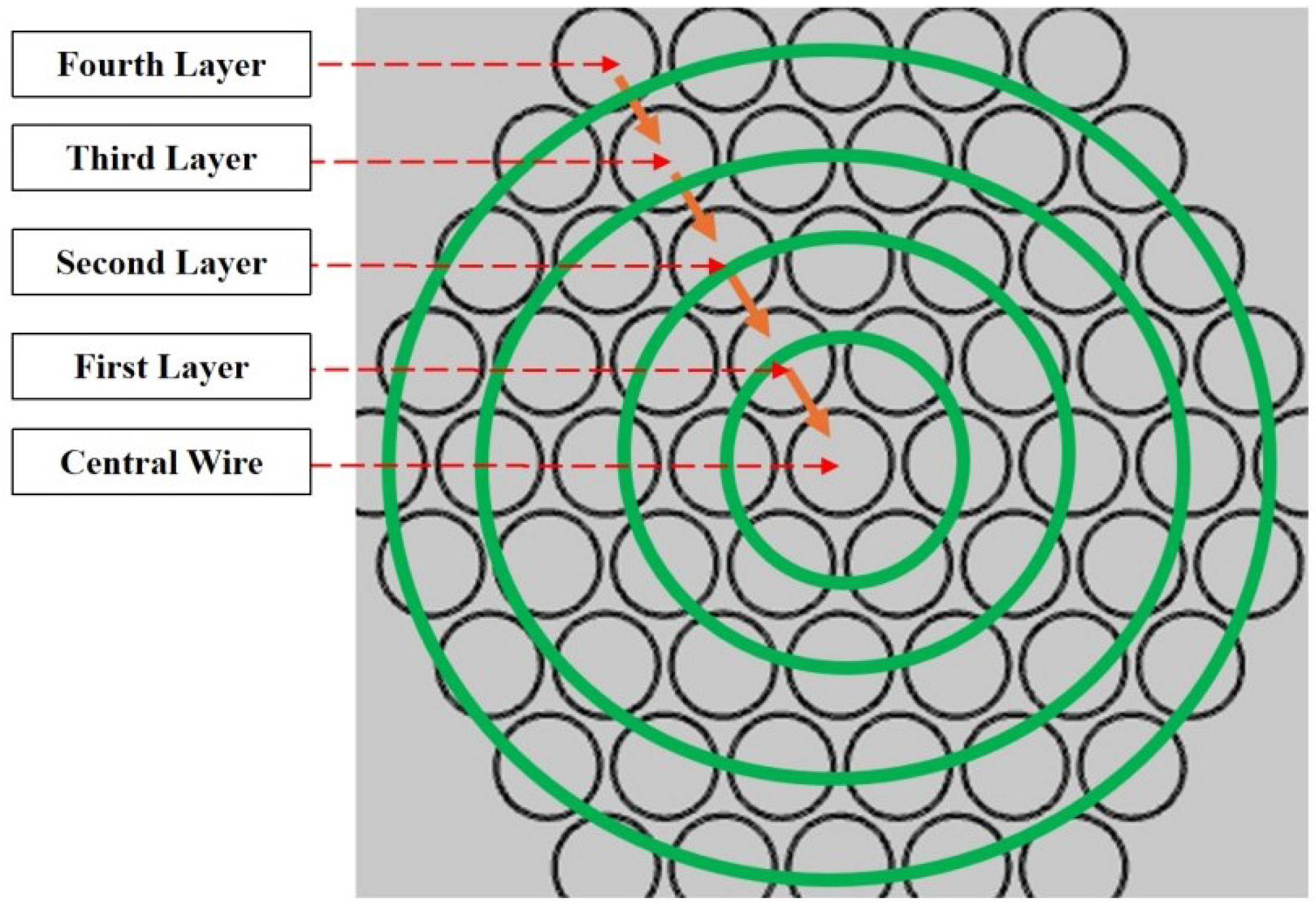
  • Transfer calculation from the outside to the inside. A current is applied from the outside to the inside, and the temperature of the outermost layer is first simulated. The outside-to-inside iteration is reflected by overwriting the initial values of the ambient temperature parameters of the inner layer. Since the steady-state temperature is calculated, the temperature influence from the outer layer to the inner layer can be calculated by the average value of the temperatures of two to three adjacent wires. Then, for the next outer layer, the average temperature of the outer layer wires is set as the ambient temperature, and the corresponding current is applied to calculate the temperature of the next outer layer in the first iteration from outside to inside. By repeating until the central wire of the harness is reached, the temperature of this wire of the harness can be obtained.
  • Transfer calculation from the inside to the outside. The average value is calculated from the outside to the inside, while the influence of the temperature of the central wire on the outer-layer wires is indicated by the temperature rise transfer from a few wires to many wires, exhibiting a clearer temperature drop. By intercepting the results of multiple groups of finite element simulations, the influence coefficients are fitted into a function of the wire specification, interval distance, and convective heat transfer coefficient as the correction coefficient for the temperature influence of each layer from inside to outside. Then, the iterative process is carried out from the inside to the outside. This influence on the thermal network is reflected in the ambient temperature in the model so as to realize the temperature simulation of the outer layer wires.

4.3. Comparison of Experimental Tests and Simulation Results

In this paper, the actual temperature rise characteristics of a wire harness are tested through experiments as reference values, and the thermal network calculation values are compared and analyzed with them. A schematic diagram of the wire harness experimental bench is shown in Figure 18, the experimental equipment is shown in Figure 19, and the experimental wire harness is shown in Figure 20. A power supply is loaded at one end of the wire, and a load is loaded at the other end. It is beneficial to conduct comparative analysis of temperature data by simultaneously using three temperature sensors for measurement. These three temperature sensors (one temperature sensor at each end of the wiring harness and one in the middle of the wiring harness) are installed on the surface of the wire harness insulation layer, and the test wires are connected to the test equipment. The test equipment transmits the test data to the display and recording equipment for analog display and recording of the test data. In the experiment, the current value applied to the wire is continuously increased from small to large, the temperature change on the wire surface is tested until the temperature rises and stabilizes at the maximum temperature that the wire can withstand, and the current value at this time is recorded. The current values when different specifications of wires reach the maximum temperature limit are repeatedly tested, and the robustness and reliability of the results are ensured through repeated experiments in batches.
Table 2 shows the thermal network analysis results of a harness composed of 37 wires. Table 3 shows the analysis results of the harness thermal network model for a harness composed of 61 wires.
Through the comparative analysis of experimental values, finite element simulation values, and thermal network values, the calculated values of the thermal network method proposed in this paper have an error of approximately 8% compared with the experimental values for complex wire harnesses. The traditional current-carrying capacity derating method can only utilize over 40% of the wiring harness’s capacity. The traditional approach continuously increases the loading current value of the wiring harness through experiments. Now, it can be quickly calculated through the heat network method, achieving weight reduction, cost reduction and efficiency improvement.
The simulation in this paper is carried out under the following computing environment: CPU model: 13th Gen Intel(R) Core(TM) i5-13400 (core count: ten cores, thread count: sixteen threads, base frequency: 2.5 GHz), memory 16 GB. In the finite element method, under this computing environment, the time for computing the harness temperature is affected by the mesh density of the single-wire model and the number of wires in the harness, with a calculation time of 10–20 min, while the thermal network method for calculating the harness model takes 1–2 min, a speed increase of more than 60%.

5. Discussion

This study lays the groundwork for the accurate, rapid, and batch calculation of the rising thermal temperature in aircraft EWIS wiring harnesses. However, the wiring harnesses investigated in this study all exhibited a straight physical configuration, and since many EWIS wiring harnesses on aircraft feature bends, it may be necessary to consider the influence of the bend radius on the temperature rise in such cases. This warrants further investigation in future research.

6. Conclusions

Aiming to balance the model speed, accuracy, and complexity for calculations of wire temperature rises in aircraft EWIS design, in this paper, we propose a harness thermal network modeling method based on thermal resistance hierarchy fusion iteration. The core contributions are as follows: by analyzing the mechanism of wire temperature rise, a thermal resistance hierarchical wire thermal network model is established and extended to the harness level. Through hierarchical modeling and inner–outer layer iterative calculation methods, the calculation accuracy requirements for harness thermal network models are met. The calculation errors for the wire harness are all within 8%, meeting the accuracy requirements, and the model’s complexity and simulation time are greatly reduced (80%). This method establishes a technical route of hierarchical decoupling modeling and dynamic fusion iteration based on high-fidelity finite element boundary input, providing an expandable engineering application scheme for the collaborative simulation of complex harness losses and temperature rises.

Author Contributions

Conceptualization, T.C., T.Z. and S.C.; methodology, T.C. and S.C.; writing, T.C.; software, T.C. and W.L.; validation, T.C. and W.L.; investigation, W.L. All authors have read and agreed to the published version of the manuscript.

Funding

This research received no external funding.

Data Availability Statement

The original contributions presented in the study are included in the article, further inquiries can be directed to the corresponding author.

Acknowledgments

Thank you to Shumei Cui and Wei Li for their help.

Conflicts of Interest

Author Tao Cao was employed by the company Commercial Aircraft Corporation of China. The remaining authors declare that the research was conducted in the absence of any commercial or financial relationships that could be construed as a potential conflict of interest.

Abbreviations

The following abbreviations are used in this manuscript:
EWISElectrical wiring interconnection system

References

  1. Hu, X. Research on Electrical Wiring Design and Verification of Civil Aircraft. In Proceedings of the 2022 2nd International Conference on Electrical Engineering and Control Science (IC2ECS), Nanjing, China, 16–18 December 2022; IEEE: Piscataway, NJ, USA, 2022; pp. 96–100. [Google Scholar]
  2. Crnko, T.; Dyrnes, S. Arc fault hazards and safety suggestions for design and maintenance. IEEE Ind. Appl. Mag. 2001, 7, 23–32. [Google Scholar] [CrossRef]
  3. Furse, C.; Haupt, R. Down to the wire. IEEE Spectr. 2001, 38, 34–39. [Google Scholar] [CrossRef]
  4. Spyker, R.; Schweickart, D.L.; Horwath, J.C.; Walko, L.C.; Grosjean, D. An evaluation of diagnostic techniques relevant to arc fault current interrupters for direct current power systems in future aircraft. In Proceedings of the Electrical Insulation Conference and Electrical Manufacturing Expo, Indianapolis, IN, USA, 23–26 October 2005; IEEE: Piscataway, NJ, USA, 2005; pp. 146–150. [Google Scholar]
  5. Cecchi, V.; Miu, K.; Leger, A.S.; Nwankpa, C. Study of the impacts of ambient temperature variations along a transmission line using temperature-dependent line models. In Proceedings of the 2011 IEEE Power and Energy Society General Meeting, Detroit, MI, USA, 24–28 July 2011; IEEE: Piscataway, NJ, USA, 2011; pp. 1–7. [Google Scholar]
  6. Cecchi, V.; Leger, A.S.; Miu, K.; Nwankpa, C.O. Incorporating temperature variations into transmission-line models. IEEE Trans. Power Deliv. 2011, 26, 2189–2196. [Google Scholar] [CrossRef]
  7. Nigol, O.; Barrett, J.S. Characteristics of ACSR conductors at high temperatures and stresses. IEEE Trans. Power Appar. Syst. 2007, 2, 485–493. [Google Scholar] [CrossRef]
  8. Sellers, S.M.; Black, W.Z. Refinements to the Neher-McGrath model for calculating the ampacity of underground cables. IEEE Trans. Power Deliv. 1996, 11, 12–30. [Google Scholar] [CrossRef]
  9. Anders, G.J.; Coates, M. Mohamed ampacity calculations for cables in shallow troughs. IEEE Trans. Power Deliv. 2010, 25, 2064–2072. [Google Scholar] [CrossRef]
  10. IEC 60287-1-1:1994; Calculation of the Current Rating of Electric Cables, Part1: Current Rating Equations (100% Load Factor) and Calculation of Losses, Section 1: General. International Electrotechnical Commission: Geneva, Switzerland, 1994.
  11. IEC 60287-2-1 AMD 1-2006; Electric Cables-Calculation of the Current Rating-Part 2-1: Thermal Resistance; Calculation of Thermal Resistance; Amendment 2. International Electrotechnical Commission: Geneva, Switzerland, 2006.
  12. Huang, X. Transmission Line Online Monitoring and Fault Diagnosis, 2nd ed.; China Electric Power Press: Beijing, China, 2013; pp. 69–194. [Google Scholar]
  13. Henke, A.; Frei, S. Transient temperature calculation in a single cable using an analytic approach. J. Fluid Flow Heat Mass Transf. (JFFHMT) 2020, 7, 58–65. [Google Scholar] [CrossRef]
  14. Henke, A.; Frei, S. Analytical Approaches for Fast Computing of the Thermal Load of Vehicle Cables of Arbitrary Length for the Application in Intelligent Fuses. In Proceedings of the VEHITS, Online, 28–30 April 2021; pp. 396–404. [Google Scholar]
  15. Benthem, R.; Grave, W.; Doctor, F.; Nuyten, K.; Taylor, S.; Routier, P.A.J.D. Thermal analysis of wiring bundles for weight reduction and improved safety. In Proceedings of the 41st International Conference on Environmental Systems, Portland, OR, USA, 17–21 July 2011; p. 5111. [Google Scholar]
  16. Lei, M.; Liu, G.; Lai, Y.-t.; Li, J.-z.; Li, W.; Liu, Y.-g. Study on thermal model of dynamic temperature calculation of single-core cable based on Laplace calculation method. In Proceedings of the 2010 IEEE International Symposium on Electrical Insulation, San Diego, CA, USA, 6–9 June 2010; IEEE: Piscataway, NJ, USA, 2010; pp. 1–7. [Google Scholar]
  17. Fu, C.; Si, W.; Zhu, L.; Li, H.; Yao, Z.; Wang, Y. Research on the fast calculation model for transient temperature rise of direct buried cable groups. In Proceedings of the 2018 12th International Conference on the Properties and Applications of Dielectric Materials (ICPADM), Xi’an, China, 20–24 May 2018; IEEE: Piscataway, NJ, USA, 2018; pp. 646–652. [Google Scholar]
  18. Xiao, R.; Liang, Y.; Fu, C.; Cheng, Y. Rapid calculation model for transient temperature rise of complex direct buried cable cores. Energy Rep. 2023, 9, 306–313. [Google Scholar] [CrossRef]
  19. Liang, Y.; Cheng, X.; Zhao, Y. Research on the rapid calculation method of temperature rise of cable core of duct cable under emergency load. Energy Rep. 2023, 9, 737–744. [Google Scholar] [CrossRef]
  20. Fu, C.Z.; Si, W.R.; Quan, L.; Yang, J. Numerical study of convection and radiation heat transfer in pipe cable. Math. Probl. Eng. 2018, 2018, 5475136. [Google Scholar] [CrossRef]
  21. Girshin, S.S.; Bubenchikov, A.A.; Bubenchikova, T.V.; Goryunov, V.N.; Osipov, D.S. Mathematical model of electric energy losses calculating in crosslinked four-wire polyethylene insulated (XLPE) aerial bundled cables. In Proceedings of the 2016 ELEKTRO, High Tatras, Slovakia, 16–18 May 2016; IEEE: Piscataway, NJ, USA, 2016; pp. 294–298. [Google Scholar]
  22. Zhou, X.; Wen, D.; Wang, S.; Liu, Y.; Jiang, Y.; Li, T. Simulation Analysis of Bundle Conductors Thermal Field in High Voltage Overhead Transmission Lines. Electrotech. Electr. 2017, 3, 20–22. [Google Scholar]
  23. Yu, X.; Yao, L.; Zhao, S.; Yu, S.; He, A. Infrared On-line Diagnosis Method for the Recessive Defects of Aviation Wire Insulation Layer. Ship Electron. Eng. 2019, 39, 199–203. [Google Scholar]
  24. Al-Dulaimi, A.A.; Guneser, M.T.; Hameed, A.A.; Márquez, F.P.G.; Gouda, O.E. Adaptive FEM-BPNN model for predicting underground cable temperature considering varied soil composition. Eng. Sci. Technol. Int. J. 2024, 51, 101658. [Google Scholar] [CrossRef]
  25. Ma, M.; Guo, W.; Yan, X.; Yang, S.; Zhang, X.; Chen, W.; Cai, G. A Three-Dimensional Boundary-Dependent Compact Thermal Network Model for IGBT Modules in New Energy Vehicles. IEEE Trans. Ind. Electron. 2021, 68, 5248–5258. [Google Scholar] [CrossRef]
  26. ISO 1302:2002; Geometrical Product Specifications (GPS)—Indication of Surface Texture in Technical Product Documentation. International Organization for Standardization: Geneva, Switzerland, 2002.
  27. Aerospace Standard. Wiring, Aerospace Vehicle AS50881. Available online: https://www.sae.org/standards/content/as50881g (accessed on 17 July 2025).
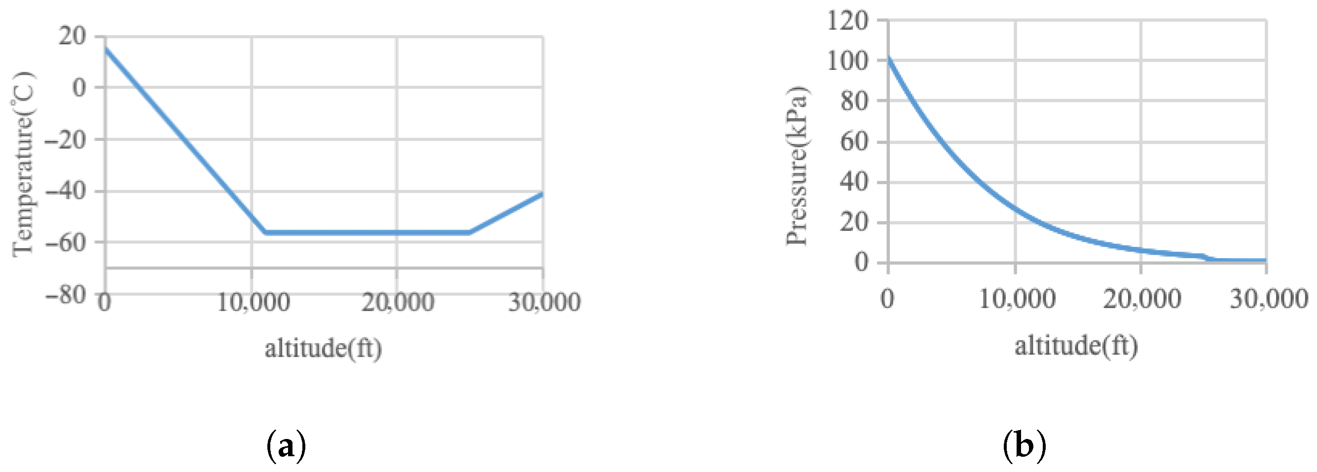
  28. National Aeronautics and Space Administration. Earth Atmosphere Model. Available online: https://www.grc.nasa.gov/WWW/K-12/airplane/atmosmet.html (accessed on 7 July 2021).
Figure 1. Building process of finite element model.
Energies 18 04046 g001
Figure 2. Finite element grid diagram.
Energies 18 04046 g002
Figure 3. Boundary setting grid diagram.
Energies 18 04046 g003
Figure 4. Fluid simulation cloud map.
Energies 18 04046 g004
Figure 5. Variation in temperature and pressure with altitude. (a) Relationship between ambient temperature and altitude. (b) Relationship between pressure and altitude.
Energies 18 04046 g005
Figure 6. Heat transfer rate of wires at different wire diameters and at different pressures.
Energies 18 04046 g006
Figure 7. Heat transfer rate of wires at different wire diameters and pressures after interpolation.
Energies 18 04046 g007
Figure 8. Variation in heat transfer rate with wire diameter at 75.35 kPa and 19.75 kPa.
Energies 18 04046 g008
Figure 9. FEM model of harness.
Energies 18 04046 g009
Figure 10. Convective heat transfer coefficients of wire harnesses with different numbers of wires.
Energies 18 04046 g010
Figure 11. Thermal network model of a traditional wire.
Energies 18 04046 g011
Figure 12. Thermal network model correction ideas.
Energies 18 04046 g012
Figure 13. Modified single-wire thermal network model.
Energies 18 04046 g013
Figure 14. Calculation method of hierarchical thermal network model (taking seven wire harnesses as an example).
Energies 18 04046 g014
Figure 15. First-layer wiring harness thermal network model.
Energies 18 04046 g015
Figure 16. Schematic diagram of the hierarchical model of the harness thermal network.
Energies 18 04046 g016
Figure 17. The process of building a harness thermal network model.
Energies 18 04046 g017
Figure 18. Schematic diagram of the experimental bench.
Energies 18 04046 g018
Figure 19. Experimental equipment.
Energies 18 04046 g019
Figure 20. Test experiment photo.
Energies 18 04046 g020
Table 1. Comparison and analysis of 260 ℃ simulation calculations and experimental data for different wires.
Wire Gauge260 ℃ Experimental Test Current (A)FEM Simulation Current (A)Thermal Network Model Simulation Current (A)FEM Model Error (%)Thermal Network Model Error (%)
AWG4284.2288.4269.71.4785.10
AWG1278.980.974.52.5355.58
AWG2030.031.828.36.0005.67
Table 2. A total of 37 AWG16 wires make up the harness analysis results.
Power-On ConditionTested (℃)FEM (℃)Thermal Network Model Simulation Current (A)FEM Model Error (%)Thermal Network Model Error (%)
Central 43.66 A
Peripheral 0 A171.01178.6180.44.45.5
Central 43.66 A
Peripheral 9.1 A260.89268.7271.63.04.1
All 10.5 A152.86158.5159.43.74.2
All 12.3 A200.2208.2210.64.05.1
All 14.1 A257.26268.1269.04.24.5
Table 3. A total of 61 AWG18 wires make up the harness analysis results.
Power-On ConditionTested (℃)FEM (℃)Thermal Network Model Simulation Current (A)FEM Model Error (%)Thermal Network Model Error (%)
Central 38.93 A
Peripheral 0 A173.82180.5185.23.8436.56
Central 38.93 A
Peripheral 6.2 A263.08271.6284.73.2398.21
All 7.4 A150.5155.1161.53.0567.31
All 8.7 A200.7207.9213.53.5876.38
All 10.05 A261.72269.4281.32.9347.49
Disclaimer/Publisher’s Note: The statements, opinions and data contained in all publications are solely those of the individual author(s) and contributor(s) and not of MDPI and/or the editor(s). MDPI and/or the editor(s) disclaim responsibility for any injury to people or property resulting from any ideas, methods, instructions or products referred to in the content.

