A Multi-Objective Decision-Making Method for Optimal Scheduling Operating Points in Integrated Main-Distribution Networks with Static Security Region Constraints

Abstract

With the increasing penetration of distributed generation (DG), integrated main-distribution networks (IMDNs) face challenges in rapidly and effectively performing comprehensive operational risk assessments under multiple uncertainties. Thereby, using the traditional hierarchical economic scheduling method makes it difficult to accurately find the optimal scheduling operating point. To address this problem, this paper proposes a multi-objective dispatch decision-making optimization model for the IMDN with static security region (SSR) constraints. Firstly, the non-sequential Monte Carlo sampling is employed to generate diverse operational scenarios, and then the key risk characteristics are extracted to construct the risk assessment index system for the transmission and distribution grid, respectively. Secondly, a hyperplane model of the SSR is developed for the IMDN based on alternating current power flow equations and line current constraints. Thirdly, a risk assessment matrix is constructed through optimal power flow calculations across multiple load levels, with the index weights determined via principal component analysis (PCA). Subsequently, a scheduling optimization model is formulated to minimize both the system generation costs and the comprehensive risk, where the adaptive grid density-improved multi-objective particle swarm optimization (AG-MOPSO) algorithm is employed to efficiently generate Pareto-optimal operating point solutions. A membership matrix of the solution set is then established using fuzzy comprehensive evaluation to identify the optimal compromised operating point for dispatch decision support. Finally, the effectiveness and superiority of the proposed method are validated using an integrated IEEE 9-bus and IEEE 33-bus test system.

1. Introduction

With the increasing penetration of distributed renewable energy (e.g., wind and photovoltaic) in power systems, traditional unidirectional distribution networks are evolving into active intelligent systems with bidirectional regulation capabilities [1,2,3]. DG’s output volatility and randomness exacerbate operational uncertainties, which brings challenges for the IMDN dispatch models with risk-awareness to enhance the practical applicability of the dispatch strategies.

In earlier research, the IMDN dispatch methods typically employed independent optimization models. While these traditional strategies could enhance local stability, they failed to achieve global optimality. Subsequently, coordinated IMDN dispatch methods were proposed to achieve fine-grained regulation of the DG output combined with energy storage control [4]. This multi-time-scale dispatch model improves the system operational economy and the renewable energy integration capacity. Ref. [5] developed a transmission–distribution collaborative optimization model to balance feasibility and efficiency using advanced solving algorithms. However, the aforementioned optimization models struggle to meet the real-time operational risk requirements when accounting for source-load uncertainties. To position the economic-risk balance as a core dispatch challenge in IMDNs, Ref. [6] proposed a risk assessment framework. This framework utilized a global system model and adaptive power flow analysis to quantify cross-voltage-level risks under fault conditions. Ref. [7] developed a risk-constrained reserve dispatch strategy to optimize energy storage coordination and power exchange. Ref. [8] constructed a dual-objective model minimizing both the operation costs and the risks for large-scale photovoltaic (PV) integration, focusing on a single security objective to achieve dynamic risk control. Ref. [9] presented a two-stage dispatch method (day-ahead and real-time) incorporating economic objectives, but its risk model relies heavily on empirically pre-set scenarios. These achievements have introduced risk-awareness mechanisms to enhance the strategy robustness. Nevertheless, the existing methods remain limited in handling dynamic load fluctuations and multi-DG coordination. Furthermore, risk assessments concerning the systemic risk of the IMDNs require improvement.

To analyze the dynamic risk changes before/after dispatch implementation, the steady-state security region (SSR) transforms the power flow constraints in the node injection space into hyperplane-based security boundary models with deterministic topology, as proposed in Ref. [10]. The SSR is characterized by precomputed hyperplane coefficients for specific network configurations. This allows the online security assessment of the power systems to bypass complex nonlinear solving.

In this context, this paper proposes a dual-objective main-distribution dispatch method for economic and risk optimization under SSR constraints. The main contributions of this paper can be summarized as follows:

(1) Employing the non-sequential Monte Carlo method to generate operating scenarios enables the efficient and comprehensive coverage of diverse potential operating states, thus facilitating the accurate identification of critical risk features, eliminating the dependence on specific operating state sequences, and ultimately enhancing the flexibility and applicability of scenario generation. Furthermore, a multi-scenario probabilistic risk assessment index system was developed, providing a solid theoretical and empirical foundation for the subsequent risk analysis and decision optimization.

(2) A hyperplane-based SSR model was derived from the nodal power flow and line current equations. This model not only accurately enforces static security constraints but also substitutes nonlinear power flow equations with linear SSR formulations, reducing the computational overhead in subsequent optimization iterations. Concurrently, principal component analysis (PCA) was employed to solve the risk assessment matrix constructed from the optimal power flow (OPF) solutions under multiple load levels, determining the inter-indicator weights; this methodology incorporates the effects of diverse load states while eliminating subjectivity in the weight determination processes, thereby ensuring an impartial and robust risk assessment.

(3) Leveraging the AG-MOPSO scheduling model—noted for rapid convergence, low computational complexity, and well-distributed solutions—the Pareto-optimal set which simultaneously minimizes the generation costs and operational risks is efficiently generated. Subsequently, fuzzy synthetic evaluation selects the optimal compromise operating point from this set, enhancing decision robustness and practicability.

The remainder of this paper is organized as follows. Section 2 introduces the risk indicators for IMDNs. Section 3 develops the integrated operation scheduling model for IMDNs. Section 4 establishes the optimal operating point decision-making based on the fuzzy comprehensive evaluation. Section 5 validates the proposed method through simulations and analyzes the results using an integrated IEEE 9-bus and IEEE 33-bus test system. Section 6 summarizes the main conclusions.

2. Establishment of Risk Indicators for IMDN

Utilizing historical operation data, equipment status, and environmental information from IMDNs, this paper extracts critical risk characteristics through multi-scenario analysis to reveal the risk formation mechanisms and establish a quantitative foundation for indicator system construction [11]. Employing extensive scenarios generated via non-sequential Monte Carlo simulation, the network topology is identified using line fault models, with the risks evaluated through power flow calculations [12]. To enable comprehensive multi-dimensional risk assessments in IMDNs, this work builds upon the extracted risk characteristics and integrates established power system risk assessment methodologies [13,14]. The selected risk assessment indicators for the transmission and distribution levels are presented below. All indicators are dimensionless, with real-time computable assessment methods established as follows.

2.1. Risk of Insufficient Reserve

$$R_P=\rho \left[{\displaystyle \frac{\exp \left(1-\frac{P_S-P_{load}^{\max }}{P_{\mathrm{load}}^{\max }}\right)-1}{\mathrm{e}-1}}\right]$$

(1)

where $R_p$ is the probability of risk occurrence in the system state; $P_S$ is the reserve capacity; $P_{load}^{max}$ load is the total maximum load of the system; $e$ is the natural constant.

2.2. Risk of Power Factor Violation

$$R_Z=\rho \left[{\displaystyle \frac{\exp \left(\frac{\max \left(\left|\mathsf{\Delta }\cos \phi \right|-\mathsf{\Delta }\cos {\phi }_{\max },0\right)}{\mathsf{\Delta }\cos {\phi }_{\max }}\right)-1}{\mathrm{e}-1}}\right]$$

(2)

where $\left|\mathrm{\Delta }cos\phi \right|$ denotes the system power factor deviation and $\mathrm{\Delta }cos{\phi }_{max}$ denotes the maximum permissible power factor deviation under normal operating conditions.

2.3. Risk of Feeder Power Overload

$$R_{FL}=\rho {\displaystyle \sum _{j=1}^{N_{FL}}\left[\frac{\exp \left(1-\frac{P_{fl,j}^{\max }-P_{fl,j}}{P_{fl,j}^{\max }}\right)-1}{\mathrm{e}-1}\right]}$$

(3)

where $R_{FL}$ is the number of main distribution network feeders in the system; $P_{fl,j}$ is the active power transmitted by the feeder $j$; $P_{fl,j}^{max}$ is the maximum active power allowed to be transmitted by the feeder $j$;

2.4. Risks of Wind and Solar Curtailment

$$R_{DG}=\rho \left[{\displaystyle \frac{\exp \left(\frac{P_{DG}^{pre}-P_{DG}}{P_{DG}^{pre}}\right)-1}{\mathrm{e}-1}}\right]$$

(4)

where $P_{DG}^{pre}$ represents the predicted total output of DG and $P_{DG}$ denotes the actual DG output in the system.

3. Integrated Operation Scheduling Model for IMDN

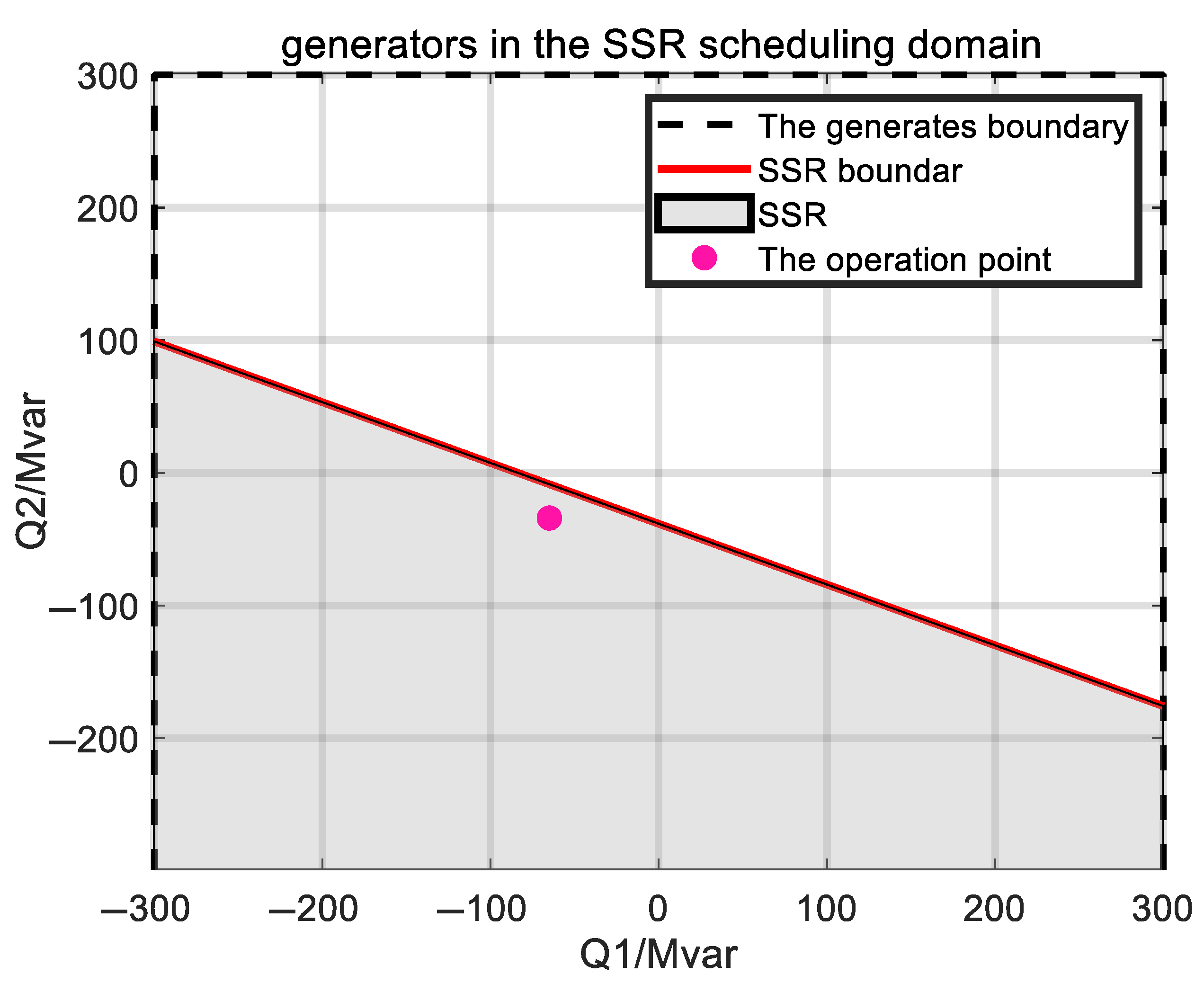
3.1. SSR Constraint Model

Assume that the power grid system consists of $n$ nodes and $n_b$ lines, where $N$ denotes the set of system nodes ($\mathrm{N} = \{1, 2, \dots , \mathrm{n}\}$), $N_G$ denotes the set of generator nodes, $N_L$ denotes the set of load nodes, and $B$ denotes the set of lines ($\mathrm{B} = \left\{{\mathrm{l}}_1, {\mathrm{l}}_2, \dots , {\mathrm{l}}_{{\mathrm{n}}_{\mathrm{b}}-1}, {\mathrm{l}}_{{\mathrm{n}}_{\mathrm{b}}}\right\}$). The injection power of each node is denoted by the vector $\chi ={\left(P_1,\dots ,P_n,Q_1,\dots ,Q_n\right)}^T\in R^{\left\{2n\right\}}$. In the context of the SSR description, the node injection powers serve as variables to characterize the static security constraints of the power system from a regional perspective. These constraints include power flow constraints, node voltage constraints, and line current constraints. The security region is defined as the set $\Omega$ of all node injection power vectors satisfying all static security constraints, i.e.,:

$$\mathrm{\Omega }=\left\{\chi \left|\begin{array}{c}{V}_i^{\mathrm{m}}⩽V_i⩽V_i^{\mathrm{M}}\\ \left|I_l\right|⩽I_l^{\mathrm{M}}\\ f(V,\theta )=x\end{array}\right.\right\}\hspace{1em}\begin{array}{c}\forall i\in N\\ \forall l\in B\end{array}$$

(5)

where $V_i$, $V_i^M$, and $V_i^m$ denote the voltage, upper magnitude limit, and lower magnitude limit of node $i$, respectively; $I_l$, $I_l^M$, and $\left|I_l\right|$ denote the current, upper magnitude limit of current, and magnitude of current for line $l$, respectively; $f(V,\theta )$ denotes the power flow equations of the system.

The specific derivation process of the SSR is shown in Appendix A.1. When $V_i-V_i^M=0$, $V_i-V_i^m=0$, and $\left|I_l\right|-I_l^M=0$, normalizing the equation yields the hyperplane representation of the SSR boundary as follows:

$$\left\{\begin{array}{c}{\displaystyle \sum _{\forall j\in N}({\alpha }_{i,j}^{V_i^m}{P}_j+{\beta }_{i,j}^{V_i^m}{Q}_j)}=1\\ {\displaystyle \sum _{\forall j\in N}({\alpha }_{i,j}^{V_i^M}{P}_j+{\beta }_{i,j}^{V_i^M}{Q}_j)}=1\\ {\displaystyle \sum _{\forall h\in N}({\alpha }_{l,h}^{I_l^M}{P}_h+{\beta }_{l,h}^{I_l^M}{Q}_h)}=1\end{array}\right.\hspace{1em}\begin{array}{c}\forall i\in N\\ \forall l\in B\end{array}$$

(6)

where ${\alpha }_{i,j}^{V_i^m},{\beta }_{i,j}^{V_i^m}$ denotes the hyperplane coefficient for the upper magnitude limit of node i’s voltage; ${\alpha }_{i,j}^{V_i^M},{\beta }_{i,j}^{V_i^M}$ denotes the coefficient for the lower magnitude limit; ${\alpha }_{I,h}^{I_l^M},{\beta }_{I,h}^{I_l^M}$ denotes the hyperplane coefficient when the current through line l reaches its magnitude limit.

To determine these coefficients, the critical operating points of the node voltages and line currents must be obtained. As the boundary hyperplane coefficients depend solely on the network topology, this study proposes a method for the node voltage critical points: numerical solutions are derived by setting the target node as a PV bus in the power flow calculations. For the line current critical points, the iterative algorithm outlined in Ref. [15] is employed to achieve precise identification.

3.2. Multi-Objective Model Construction Based on SSR

3.2.1. Objective Function

Minimize the generation cost:

$$F_1={\displaystyle \sum _{t=1}^T{\displaystyle \sum _{\forall g\in N_G}(a_g{P}_{g,t}^2+b_g{P}_{g,t}+c_g)}}$$

(7)

where $a_g$, $b_g$, and $c_g$ denote the fuel consumption characteristic curve parameters of generator $g$; $P_{g,t}$ denotes the active power output of generator $g$ at time $t$.

Minimize the comprehensive operational risk of IMDN:

$$F_2={\displaystyle \sum _{t=1}^{\mathrm{T}}\left({\alpha }_1{R}_P+{\alpha }_2{R}_Z+{\alpha }_3{R}_{FL}+{\alpha }_4{R}_{DG}\right)}$$

(8)

where $\alpha$ denotes the operational risk weighting coefficients, satisfying ${\alpha }_1+{\alpha }_2+{\alpha }_3+{\alpha }_4=1$.

The method for determining the weighting coefficients $\alpha$ is as follows: First, solve the Optimal Alternating Current Power Flow Model under different load levels, then construct an operational risk assessment matrix, and finally derive the coefficients via PCA as presented in Ref. [16].

3.2.2. Constraints

(a) SSR constraints:

$$\left\{\begin{array}{c}{\displaystyle \sum _{\forall j\in N}({\alpha }_{i,j}^{V_i^m}{P}_j^{\Sigma }+{\beta }_{i,j}^{V_i^m}{Q}_j)}\le 1\\ {\displaystyle \sum _{\forall j\in N}({\alpha }_{i,j}^{V_i^M}{P}_j^{\Sigma }+{\beta }_{i,j}^{V_i^M}{Q}_j)}\le 1\\ {\displaystyle \sum _{\forall h\in N}({\alpha }_{l,h}^{I_l^M}{P}_h^{\Sigma }+{\beta }_{l,h}^{I_l^M}{Q}_h)}\le 1\end{array}\right.\hspace{1em}\begin{array}{c}\forall i\in N\\ \forall l\in B\end{array}$$

(9)

$$P_k^{\Sigma }=P_k+P_{wind,k}+P_{V,k}\hspace{1em}\forall k\in N_L$$

(10)

where the injected power $P_k$ at load bus $k$ is typically denoted by a negative value; $P_{wind,k}$ denotes the wind power output at bus $k$, and $P_{V,k}$ denotes the photovoltaic power output at bus $k$. $P_j^{\sum }$ denotes the equivalent injected power at bus $k$.

(b) Power balance constraint:

As network losses constitute a negligible fraction of the total system power, they are omitted in the formulation of balance constraints.

$$\left\{\begin{array}{c}{\displaystyle \sum _{i=1}^N{P}_i}=0\\ {\displaystyle \sum _{i=1}^N{Q}_i}=0\end{array}\right.$$

(11)

Bus injected power constraint:

$$\left\{\begin{array}{c}{P}_i^m\le P_i\le P_i^M\\ Q_i^m\le Q_i\le Q_i^M\end{array}\right.$$

(12)

where $P_i^m$ and $P_i^M$ denote the minimum and maximum values of active power injection at bus $i$, respectively; $Q_i^m$ and $Q_i^M$ denote the minimum and maximum values of reactive power injection at bus $i$, respectively.

Power output constraints of DG:

$$\left\{\begin{array}{c}{P}_{wind,k}^{\min }\le P_{wind,k}\le P_{wind,k}^{\max }\\ P_{V,k}^{\min }\le P_{V,k}\le P_{V,k}^{\max }\end{array}\right.$$

(13)

where $P_{wind,k}^{max}$ and $P_{wind,k}^{min}$ denote the maximum and minimum wind power outputs connected to node $k$; $P_{V,k}^{max}$ and $P_{V,k}^{min}$ denote the maximum and minimum photovoltaic power outputs connected to node $k$.

Generator ramp rate constraints:

$$P_{g,t}-P_{g,t-1}\le R_g^{\mathrm{u}}$$

(14)

where $R_g^u$ denotes the ramp rate of generator $g$.

(c) Modification of objective function:

To optimize the objective function more effectively in the optimization algorithm, the penalty-function method can be introduced to transform it into an unconstrained problem.

$$\min {\Phi }_k(x,\mu )=f_k(x)+\mu \left[{\displaystyle \sum _{i=1}^m{h}_i^2}(x)+{\displaystyle \sum _{j=1}^n{\left(\max (0,g_j(x))\right)}^2}\right]$$

(15)

where ${\varphi }_k(x,\mu )$ denotes the modified objective function; $f_k\left(x\right)$ denotes the original objective function; $h_i\left(x\right)$ denotes the i-th equality constraint function; $g_j\left(x\right)$ denotes the j-th inequality constraint function; $m, n$ denote, respectively, the number of equality constraints and the number of inequality constraints.

3.3. Model Solution

This paper utilizes the AG-MOPSO algorithm to generate a set of operating point solutions [17]. Compared to the traditional particle swarm optimization algorithms, this method balances the breadth of global exploration and the depth of local exploitation, demonstrating a faster convergence speed and a higher solution accuracy. The detailed procedure is as follows:

(1)

IMDN operation data are input, and AG-MOPSO parameters are initialized.

(2)

After determining each particle’s position based on base-case constraints, the objective function values are calculated as particle fitness. Personal best solutions for particles are initialized, followed by evaluating the Pareto dominance relationships among the particles to construct the initial non-dominated solution set.

(3)

Using the adaptive grid method and roulette wheel selection, the global optimal solution is extracted from the non-dominated set, and the particle positions are updated accordingly.

(4)

Penalty functions are applied to each objective function under base-case constraints to compute the modified objective values. The personal best solutions are then updated, with synchronous maintenance of the non-dominated solution set.

(5)

While the size of the non-dominated set exceeds its capacity, redundant solutions are pruned based on the grid density.

(6)

The iteration count is accumulated. If the maximum iteration number is reached, the non-dominated solution set is output; otherwise, the process returns to Step 3 for further iteration.

4. Optimal Operating Point Decision-Making Based on Fuzzy Comprehensive Evaluation

4.1. Weight Determination of Evaluation Indicators

The comprehensive evaluation indicators of the system, incorporating the generation costs and various risk metrics, are presented in

Table 1. Comprehensive evaluation index system of the main-distribution network system.

Objective Layer	Criterion Layer	Index Layer
Main-Distribution Integration	Riskiness	Insufficient Reserve Risk
		Power Factor Violation Risk
		Feeder Power Overload risk
		Wind and Solar Curtailment Risk
	Economy	Power Generation Cost

. This section first employs the Analytic Hierarchy Process (AHP) and the entropy weight method to calculate the synthetic weights for each criterion-layer indicator listed in Table 1 [18]. Subsequently, the weights for the lower-level indicators in the indicator layer are derived through this combined approach. The specific calculation formulas are shown in Appendix A.2.

Determination of Weights for Each Indicator

The weights of each indicator are derived from the synthesis of the criteria layer weight vector ${\omega }_{c,i}$ and the corresponding indicator layer weight vector. The calculation formula is as follows:

$${\mathrm{\Omega }}_i={\omega }_{c,i}*{{\rm X}}_{I,i}$$

(16)

where $X_{I,i}$ denotes the weight of each indicator under the i-th criteria layer; ${\Omega }_i$ denotes the weight of each indicator under the index layer.

4.2. Construction of Fuzzy Evaluation Model

An evaluation factor set $U=\{R_P,{R_Z,R}_{FL},R_{DG},M_1\}$ for scheduling optimization decision-making is constructed. This study specifies four evaluation grades for each risk factor: excellent, good, fair, and poor, with corresponding score values of $\{90,80,60,50\}$. The threshold values for the indicator scoring grades can be adjusted appropriately according to the specific characteristics of different research objects.

The membership matrix R for each operating state in the solution set of operating points is calculated using the distribution function method to achieve fuzzification of the quantitative indicators. By integrating the weights of the evaluation indicators, a comprehensive score is derived [19].

$$\left\{\begin{array}{c}{B}_n=\mathrm{\Omega }\ast R_n=\left\{b_1^n,b_2^n,b_3^n,b_4^n,b_5^n,b_6^n\right\}\\ S_n=v\ast B_n^T\end{array}\right.$$

(17)

where $R_n$ and $B_n$ denote the membership matrix and fuzzy vector of the n-th operating point, respectively; $b_i^n$ denotes the i-th fuzzy factor in the fuzzy vector of the n-th operating point; $S_n$ denotes the comprehensive score of the n-th operating point.

Using the optimal operating point decision-making method proposed in this paper, an operating point solution set that integrates comprehensive risk and power generation costs is obtained to determine the optimal system operating point. The detailed process is illustrated in Figure 1.

5. Simulation and Result Analysis

5.1. Basic Information of Simulation

The case study in this paper utilizes a main-distribution network structure integrated with distributed photovoltaic systems, with its topology depicted in Figure 2. The main network employs the IEEE 9-node system, while the distribution network adopts the IEEE 33-node system. Connected to the main network at nodes 5, 7, and 9, the distribution network integrates the photovoltaic units at nodes 15, 20, and 24 with a photovoltaic penetration rate of 0.4. Wind turbines are connected at nodes 11 and 30, while interruptible loads are installed at nodes 2, 4, and 8 of each distribution network, with a total interruptible load of 0.08 per unit in each network. System specifications include a main network base voltage of 345 kV, a distribution network base voltage of 12.66 kV, a 100 MV·A power base value, and a maximum load of 480 MW.

Using the risk criteria defined in Section 2.1, 30,000 data samples are generated via the line fault, DG output, and load probability models, incorporating Monte Carlo simulations and power flow calculations, with a running time of 452.7 s. Of these, 8010 samples indicate risk occurrences, yielding a system risk probability of 0.267. Given the equal significance assigned to network loss and risk in this study, their subjective weight coefficients are each determined as 0.5 using the AHP.

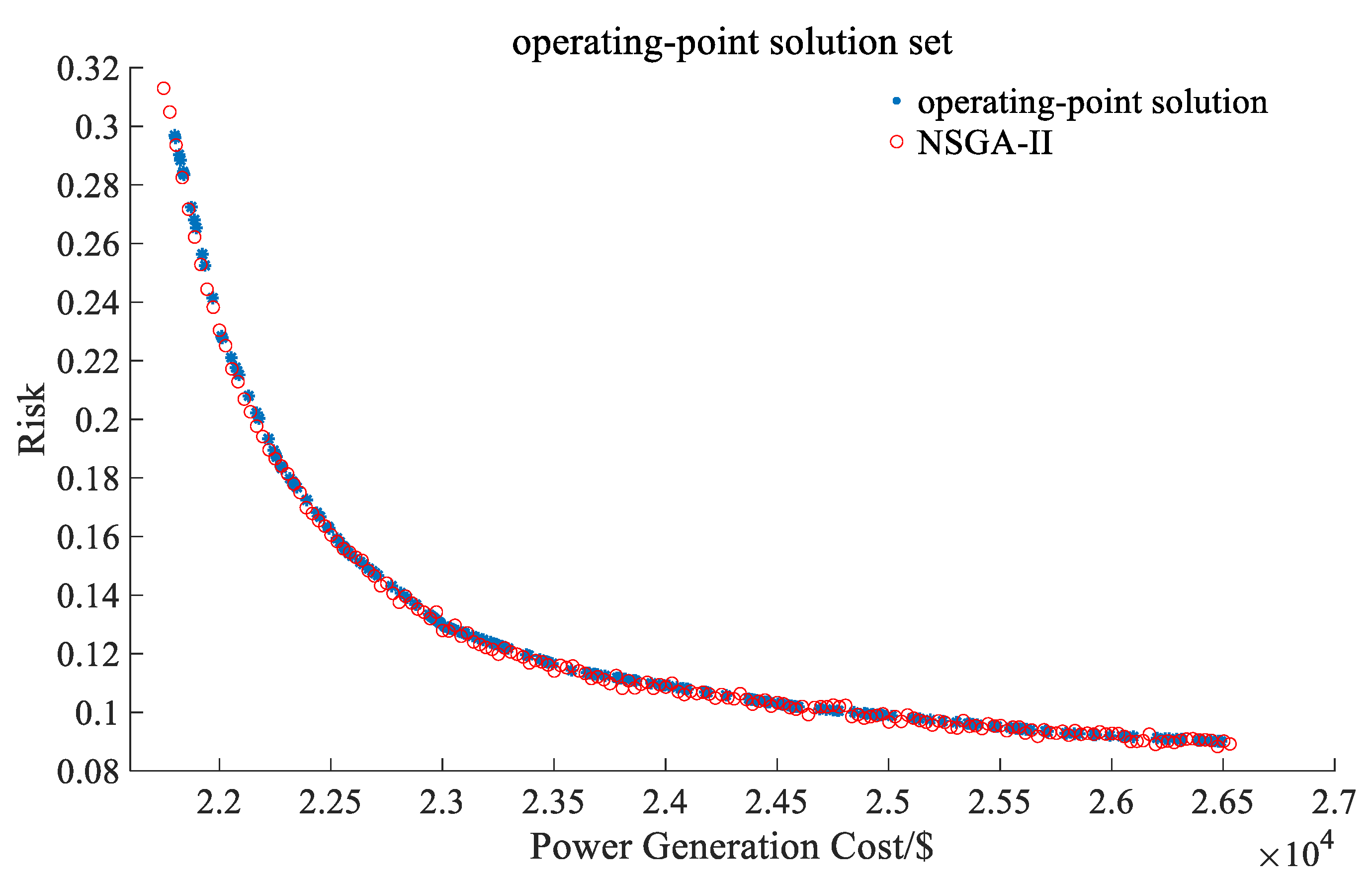
5.2. Simulation Result

Within the constraints of the SSR, optimal power flow equations under various load levels are solved to construct a risk assessment matrix for the grid under varying load conditions. PCA is then applied to determine the weight coefficients of each risk, with the results listed in

Table 2. Weight coefficient of each risk indicator.

Risk Index	Weight
$R_P$	0.31
$R_Z$	0.19
$R_{FL}$	0.23
$R_{DG}$	0.27

.

The AG-MOPSO algorithm is employed to solve the bi-objective model of power generation cost and risk, yielding a distribution curve of operating point solutions as depicted in Figure 3. For a comparative analysis, NSGA-II serves as the benchmark algorithm. As an example, the results for the first hour are presented below.

Figure 3 demonstrates a significant inverse correlation between the power generation cost and the risk parameters: a decrease in the power generation cost corresponds to an upward trend in the operational risk parameters, with their dynamic interactions forming a strong coupling relationship. This trade-off characteristic indicates that single-indicator optimization may compromise the system’s operational stability margin. To address this trade-off, a balanced mechanism integrating power generation cost control and network loss risk constraints is proposed. This mechanism requires optimizing the generating unit outputs within equipment safety boundaries to achieve economic resource allocation while implementing real-time system stability monitoring via a dynamic risk assessment model, thereby determining a scheduling strategy for dual-objective synergistic optimization within the technical feasible domain.

The power output of the generators at the optimal operating point is shown in Figure 4 and Figure 5.

To further verify the feasibility and regulation capability of the solution set under static security region (SSR) constraints, Figure 4 and Figure 5 illustrate the distributions of the active and reactive power outputs from the generators across different operating points. Figure 4 shows that the active power outputs adapt flexibly within the SSR boundaries to meet load demands, balancing the economic efficiency and operational constraints. Figure 5 reveals diverse reactive power outputs, reflecting the model’s ability to maintain voltage stability through dynamic reactive support.

These results indicate a strong nonlinear coupling between generation cost and risk: reducing one often leads to an increase in the other. This trade-off underscores the necessity of multi-objective coordination, as optimizing a single indicator may jeopardize the system stability. The output distributions in Figure 4 and Figure 5 provide a physical basis for evaluating each operating point and pave the way for selecting the optimal compromise solution through fuzzy comprehensive evaluation in the next section.

5.3. Optimal Decision Making Based on Fuzzy Comprehensive Analysis

Using the operating point solution set, the objective weights of the power generation cost and risk are determined as 0.53 and 0.47, respectively, via the entropy weight method. By applying Equation (A9), the comprehensive weights for the network loss and risk are further calculated as 0.515 and 0.485.

Scores for the operating point solution set derived from the fuzzy comprehensive evaluation method are presented in the following

Table 3. Optimal operating points for each time period.

Time/h	AG-MOPSO		NSGA-II		Time/h	AG-MOPSO		NSGA-II
	Operating Point	Score	Operating Point	Score		Operating Point	Score	Operating Point	Score
1	106	83.7	110	83.1	13	100	87.5	132	86.5
2	16	83.8	25	82.9	14	10	87.5	34	86.8
3	23	84.2	26	83.6	15	82	82.0	156	81.2
4	28	84.4	18	84.6	16	67	83.1	89	81.1
5	19	84.5	35	83.6	17	160	81.0	152	81.0
6	9	83.3	23	82.8	18	174	78.5	157	77.5
7	115	81.1	65	80.5	19	81	77.2	65	76.4
8	139	81.4	113	80.1	20	45	76.3	63	76.0
9	20	82.1	31	81.8	21	144	76.0	158	75.3
10	54	87.4	64	87.4	22	31	77.0	43	76.1
11	78	87.2	85	86.9	23	151	80.0	187	80.3
12	155	88.2	143	87.7	24	73	82.3	96	81.4

.

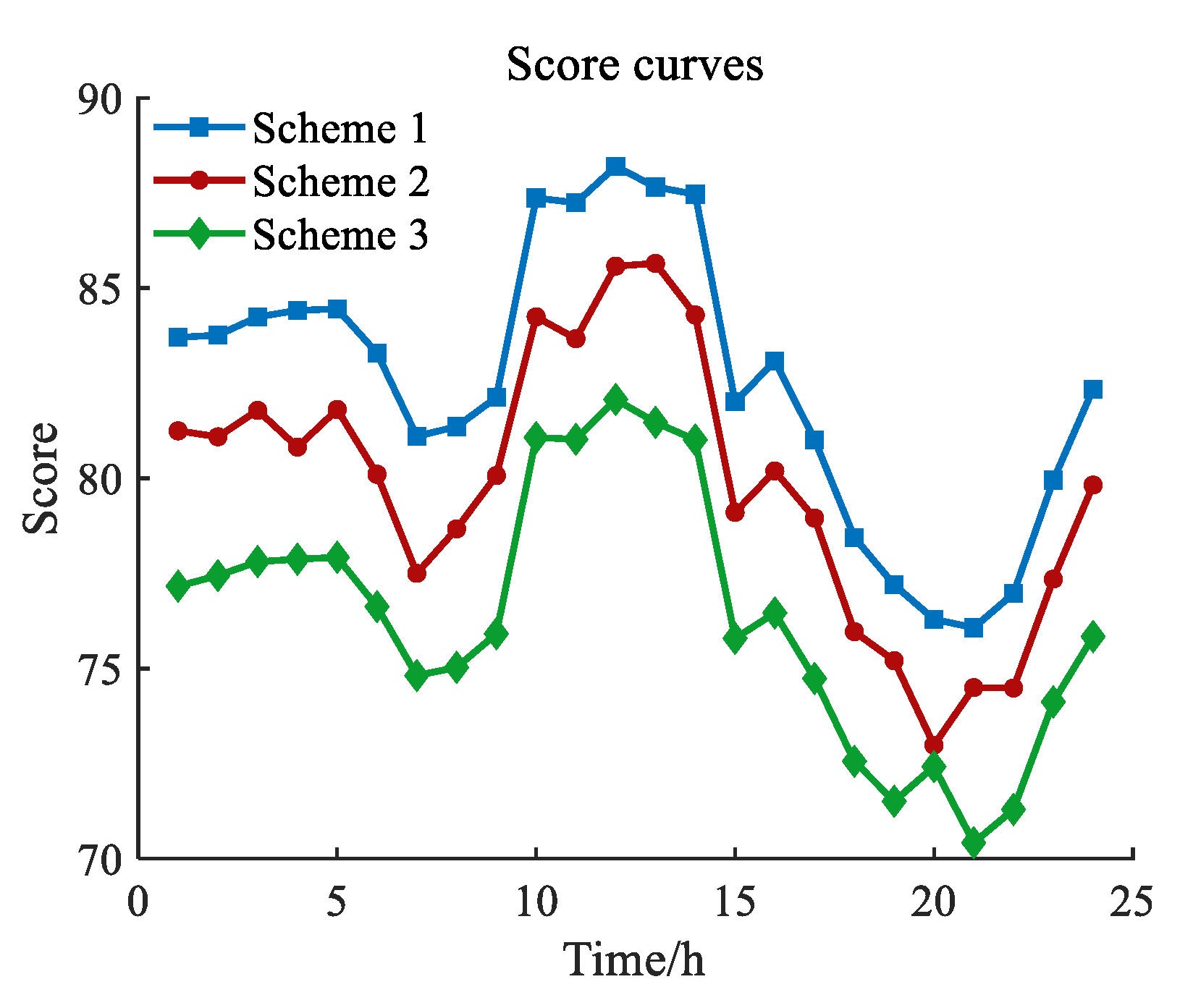
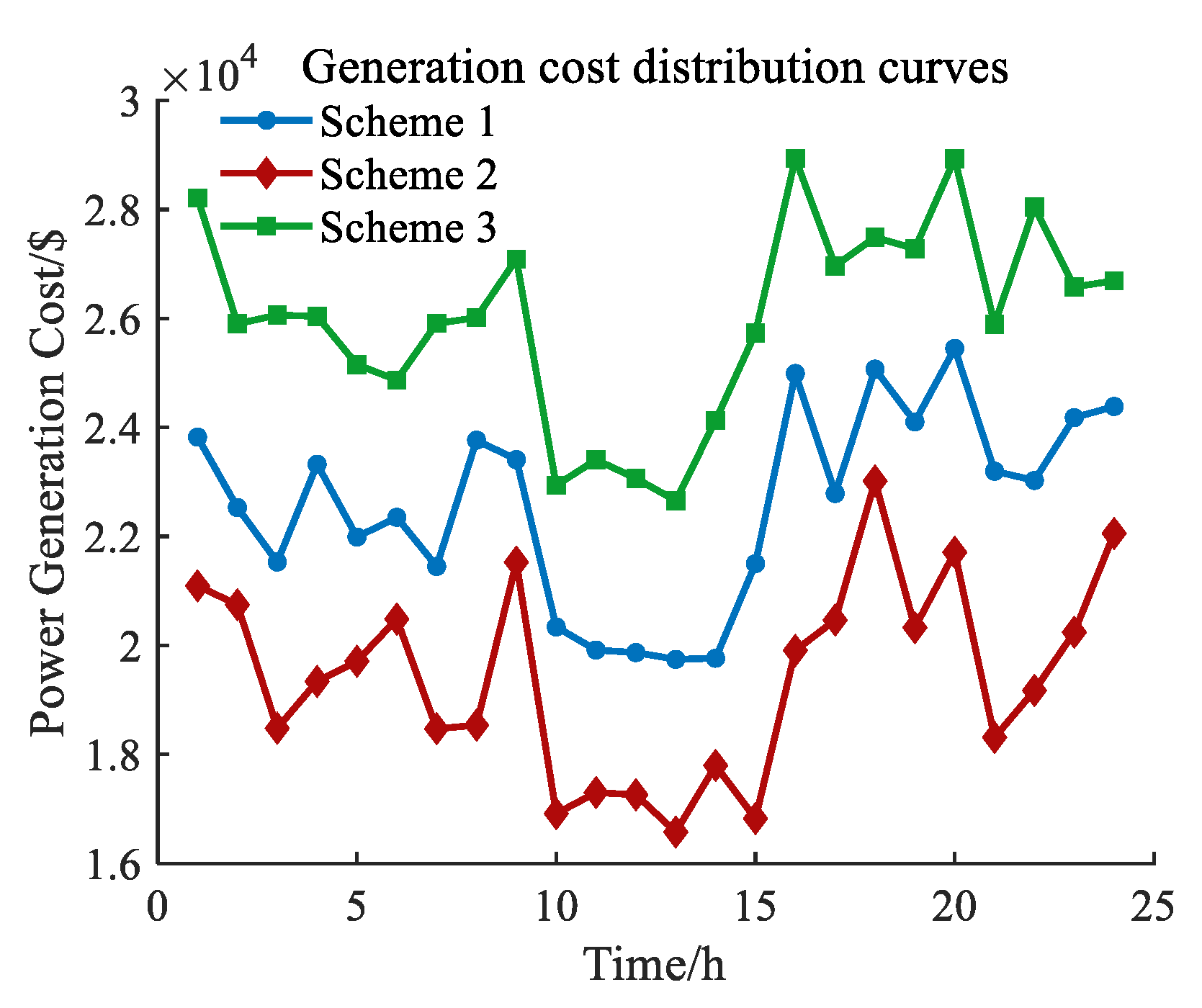
5.4. Comparative Analysis of Different Scheduling Schemes

To verify the feasibility of the proposed model in this paper, three scheduling schemes are employed under the same scenario to compare the power generation cost, the main-distribution network operation risk, and the comprehensive scores of day-ahead hourly operating points.

Scheme 1: Both the main-distribution network operation risk and the power generation cost are considered in the scheduling strategy.

Scheme 2: Power generation cost is not considered, and only the main-distribution network operation risk is taken into account in the scheduling strategy.

Scheme 3: Main-distribution network operation risk is not considered, and only the power generation cost is considered in the scheduling strategy.

The operating parameters and running time of the AG-MOPSO and NSGA-II scheduling models are presented in the table below.

As evidenced in

Table 4. Operational performance of the scheduling model.

Algorithm	Swarm Size/ Population Size	Number of Iterations	Running Time/s
AG-MOPSO	150	2000	545.4
NSGA-II	150	2000	685.3

, the AG-MOPSO algorithm exhibits a 26.3% reduction in the total runtime compared to NSGA-II. Table 3 further demonstrates that, on an hourly timescale, the Pareto-optimal solutions generated by AG-MOPSO consistently outperform those of NSGA-II in terms of operational efficiency. These findings collectively indicate that AG-MOPSO is better suited for the proposed operational strategy in practical engineering applications.

The results of the comparative analysis are shown in Figure 6, Figure 7 and Figure 8, where the operating points at each time instance are the optimal points selected via the fuzzy comprehensive evaluation.

Simulation curve analysis (e.g., Figure 4, Figure 5 and Figure 6) indicates that the system generation cost exhibits a significant downward trend during the high-penetration operation of DG between 10:00 and 15:00. This phenomenon originates from an effective reduction in the generator output by the distributed photovoltaic power. Different scheduling schemes demonstrate distinct characteristics: Scheme 1 prioritizes generation cost minimization at the expense of relaxing the system security constraints; Scheme 2 achieves safety-level optimization through enhanced risk control but causes a significant deterioration in the economic indicators; Scheme 3 employs an economic-risk synergistic control strategy to achieve a dynamic balance between economy and safety while moderately increasing the network generation costs. Comparative analysis shows that the scheduling strategy developed via the multi-objective synergistic optimization algorithm can accurately identify the optimal trade-off point on the economy–safety Pareto frontier, verifying the practical engineering value of the main-distribution network coordinated optimization model in high-proportion new energy integration scenarios.

As shown in Figure 6, Scheme 2 outperforms Scheme 3. Comparative data from Figure 7 and Figure 8 reveal that while Scheme 3 achieves a 33.83% reduction in the power generation cost, Scheme 2 decreases the operational risk level by 71.67%; this significant risk control improvement ultimately boosts Scheme 2’s comprehensive score by 4.51%. In Scheme 1, the power generation cost is 16.35% lower than in Scheme 2. Despite a 59.10% increase in risk indicators, this still achieves a 3.38% performance improvement through multi-dimensional comprehensive evaluation. These results indicate that integrating a dynamic mechanism balancing the power generation cost and the operational risk into the objective function effectively balances the system economy and safety, offering a novel technical pathway for secure and economic grid operation.

Overall, the dual-objective optimization of the power generation cost and operational risk proposed in this study effectively reduces the power generation costs and operational risks while enhancing the economic efficiency and security of the system operations. The proposed optimization method for risk-informed operating points in main and distribution networks under static security region constraints enables comprehensive scoring of the system operating states, the selection of optimal operating points, and assists grid dispatchers in making informed decisions, thereby demonstrating practical engineering value.

6. Discussion

The paper establishes a dispatch feasible domain incorporating SSR constraints, which converts nonlinear power flow constraints into linear formulations, significantly improving the system response speed. The AG-MOPSO algorithm solves multi-objective dispatch problems under SSR constraints, enabling the efficient exploration of the optimal operating points while ensuring dispatch timeliness and accuracy. A fuzzy comprehensive evaluation mechanism further optimizes the multi-objective solution set, enhancing decision-making quality.

These three components form an integrated framework: SSR defines the constrained dispatch space, AG-MOPSO generates solution sets within this space, and fuzzy evaluation selects the optimal dispatch point.

However, this method currently has the following limitations: Validation using only IEEE 9/33 bus systems, leaving algorithm scalability unverified for larger transmission–distribution networks; Independent Monte Carlo simulation of the renewable generation uncertainty, neglecting source correlations and temporal dynamics; Empirical threshold setting in fuzzy evaluation without operational data support.

To address the above issues, future research will be carried out on the following aspects: Test scalability using IEEE 118-bus and regional grid systems; Improve uncertainty modeling with time-series analysis and correlated sampling; Enhance fuzzy evaluation through data-driven calibration; Implement the method in cloud-edge architectures for real-time performance optimization.

The above improvements will further enhance the practical adaptability and engineering promotion value of the proposed method in complex and dynamic power grid environments.

7. Conclusions

To address the economy–risk trade-off in IMDNs with high-proportion DG integration, this paper proposes a coordinated optimal scheduling framework incorporating static security region constraints. A dual-objective decision-making model is established for economy and risk, employing the AG-MOPSO algorithm to rapidly generate operating point solution sets. The fuzzy comprehensive evaluation method then scores these solutions to select the optimal operating point, enabling the effective balancing of IMDN losses and risks. Simulation results demonstrate that this approach substantially reduces the system operational costs while enhancing the grid stability and safety, providing theoretical and methodological support for operating IMDNs with high-proportion DG.

References

1. Zhao, Y.; Zhang, G.; Hu, W.; Huang, Q.; Chen, Z.; Blaabjerg, F. Meta-Learning Based Voltage Control for Renewable Energy Integrated Active Distribution Network Against Topology Change. IEEE Trans. Power Syst. 2023, 38, 5937–5940. [Google Scholar] [CrossRef]
2. Poudyal, A.; Poudel, S.; Dubey, A. Risk-Based Active Distribution System Planning for Resilience Against Extreme Weather Events. IEEE Trans. Sustain. Energy 2023, 14, 1178–1192. [Google Scholar] [CrossRef]
3. Tao, Y.; Qiu, J.; Lai, S.; Sun, X.; Liu, H.; Zhao, J. Distributed Adaptive Robust Restoration Scheme of Cyber-Physical Active Distribution System With Voltage Control. IEEE Trans. Power Syst. 2024, 39, 2170–2184. [Google Scholar] [CrossRef]
4. Wang, G.; Wang, C.; Feng, T.; Wang, K.; Yao, W.; Zhang, Z. Day-Ahead and Intraday Joint Optimal Dispatch in Active Distribution Network Considering Centralized and Distributed Energy Storage Coordination. IEEE Trans. Ind. Appl. 2024, 60, 4832–4842. [Google Scholar] [CrossRef]
5. Fan, G.; Lin, S.; Feng, X.; Wang, Q.; Liu, M. Stochastic Economic Dispatch of Integrated Transmission and Distribution Networks Using Distributed Approximate Dynamic Programming. IEEE Syst. J. 2022, 16, 5985–5996. [Google Scholar] [CrossRef]
6. Tang, K.; Dong, S.; Huang, J.; Ma, X. Operational Risk Assessment for Integrated Transmission and Distribution Networks. CSEE J. Power Energy Syst. 2023, 9, 2109–2120. [Google Scholar]
7. Li, X.; Han, X.; Yang, M. Risk-Based Reserve Scheduling for Active Distribution Networks Based on an Improved Proximal Policy Optimization Algorithm. IEEE Access 2023, 11, 15211–15228. [Google Scholar] [CrossRef]
8. Liang, Z.; Kang, C.; Sui, L.; Yu, R.; Jia, Y.; Du, Y.; Chen, W. Research on operation risk assessment and prevention and control strategy of main distribution network with high proportion of distributed photovoltaic. J. Tsinghua Univ. (Nat. Sci. Ed.) 2024, 64, 1964–1978. (In Chinese) [Google Scholar]
9. Tang, Y.; Sun, D.; Zhou, Y.; Zhou, L. Research on day-ahead-real-time coordinated risk scheduling method for integrated main distribution network with distributed generation. Smart Power 2020, 48, 8–14+23. (In Chinese) [Google Scholar]
10. Yu, Y.; Liu, Y.; Qin, C.; Yang, T. Theory and Method of Power System Integrated Security Region Irrelevant to Operation States: An Introduction. Engineering 2020, 6, 754–777. [Google Scholar] [CrossRef]
11. Shi, X.; Qiu, R.; Mi, T.; He, X.; Zhu, Y. Adversarial Feature Learning of Online Monitoring Data for Operational Risk Assessment in Distribution Networks. IEEE Trans. Power Syst. 2020, 35, 975–985. [Google Scholar] [CrossRef]
12. Dechgummarn, Y.; Fuangfoo, P.; Kampeerawat, W. Reliability Assessment and Improvement of Electrical Distribution Systems by Using Multinomial Monte Carlo Simulations and a Component Risk Priority Index. IEEE Access 2022, 10, 111923–111935. [Google Scholar] [CrossRef]
13. Wang, H.; Liu, Z.; Liang, Z.; Huo, X.; Yu, R.; Bian, J. Multi-timescale risk scheduling for transmission and distribution networks for highly proportional distributed energy access. Int. J. Electr. Power Energy Syst. 2024, 155, 109598. [Google Scholar] [CrossRef]
14. Tang, M.; Li, R.; Zhang, R.; Yang, S. Research on New Electric Power System Risk Assessment Based on Cloud Model. Sustainability 2024, 16, 2014. [Google Scholar] [CrossRef]
15. Yang, T.; Yu, Y. Static Voltage Security Region-Based Coordinated Voltage Control in Smart Distribution Grids. IEEE Trans. Smart Grid 2018, 9, 5494–5502. [Google Scholar] [CrossRef]
16. Cai, L.; Thornhill, N.F.; Kuenzel, S.; Pal, B.C. Wide-Area Monitoring of Power Systems Using Principal Component Analysis and k-Nearest Neighbor Analysis. IEEE Trans. Power Syst. 2018, 33, 4913–4923. [Google Scholar] [CrossRef]
17. Han, H.; Lu, W.; Zhang, L.; Qiao, J. Adaptive Gradient Multiobjective Particle Swarm Optimization. IEEE Trans. Cybern. 2018, 48, 3067–3079. [Google Scholar] [CrossRef]
18. Wu, J.; Wang, H.; Wang, W.; Zhang, Q. Performance evaluation for sustainability of wind energy project using improved multi-criteria decision-making method. J. Mod. Power Syst. Clean Energy 2019, 7, 1165–1176. [Google Scholar] [CrossRef]
19. Li, Y.; Sun, Z.; Han, L.; Mei, N. Fuzzy Comprehensive Evaluation Method for Energy Management Systems Based on an Internet of Things. IEEE Access 2017, 5, 21312–21322. [Google Scholar] [CrossRef]
20. Sun, D.; Yu, Y. Accurate Identification of Critical Boundary Hyperplanes of Practical Steady-State Security Region in Distribution Grids. IEEE Trans. Smart Grid 2023, 14, 4312–4321. [Google Scholar] [CrossRef]
21. Wang, C.; Chu, S.; Ying, Y.; Wang, A.; Chen, R.; Xu, H.; Zhu, B. Underfrequency Load Shedding Scheme for Islanded Microgrids Considering Objective and Subjective Weight of Loads. IEEE Trans. Smart Grid 2023, 14, 899–913. [Google Scholar] [CrossRef]
22. Liu, R.; Yang, T.; Sun, G.; Lin, S.; Li, F.; Wang, X. Multi-Objective Optimal Scheduling of Community Integrated Energy System Considering Comprehensive Customer Dissatisfaction Model. IEEE Trans. Power Syst. 2023, 38, 4328–4340. [Google Scholar] [CrossRef]
23. Hua, H.; Shi, J.; Chen, X.; Yu, K.; Qin, Y.; Shen, J.; Ding, Y.; He, D. Low-carbon economic energy routing strategy based on adaptive shape estimation multi-objective evolutionary algorithm. Chin. J. Electr. Eng. 2025, 45, 1394–1409. (In Chinese) [Google Scholar]
Figure 1. Optimal operating point decision flow chart.
Energies 18 04018 g001
Figure 2. Example power grid topology diagram.
Energies 18 04018 g002
Figure 3. Operation point solution set distribution curve.
Energies 18 04018 g003
Figure 4. Active power operating points of generators in the SSR scheduling domain.
Energies 18 04018 g004
Figure 5. Reactive power operating points of generators in the SSR scheduling domain.
Energies 18 04018 g005
Figure 6. Score curves distribution for each scheme and time period.
Energies 18 04018 g006
Figure 7. Generation cost distribution curves for each scheme and time period.
Energies 18 04018 g007
Figure 8. Risk distribution curves for each scheme and time period.
Energies 18 04018 g008