A Reduced Order Model of the Thermal Profile of the Rolls for the Real-Time Control System

Abstract

Effective real-time control systems require fast and accurate models. The thermal profile models of the rolls presented in this paper are proposed for a real-time control system for the design of the rolling schedule. The thermal profile of the roll defines the shape of the roll surface, its convexity, and, finally, the shape of the final product of the flat rolling, its convexity, and flatness. This paper presents accurate semi-analytical and finite element (FE) models, which serve to obtain an accurate solution of the joint thermal and mechanical problem, that is, heat transfer and thermal expansion. The results of the FE simulation are used for training the developed thermal model based on the neural network (NN) and for the creation of a dynamic reduced order model (ROM) of the roll surface profile. The pre-trained NN model gives accurate results and is faster than the FE model, but the model is not very useful for fast calculations in a real-time control system, mainly because the temperature distribution inside the rolls is not explicitly used in further calculations. In contrast, the ROM is fast and accurate and provides surface-shaped results that can be immediately used by other models of the real-time control system. The results of the simulation of the real process are also shown. Calculations of the roll campaign (more than 9 h) by the FEM model last several hours, while by the ROM less than 20 s.

1. Introduction

Modeling of the process becomes more accurate and takes into account more factors and less important phenomena. The complexity and dimension of the models are constantly arising. Many advanced mathematical models are difficult or impossible to use in real-time processes. To reduce computational complexity, for example, in control systems simulations, model order is reduced. Such a model replaces the original complex model and is commonly called a reduced-order model (ROM). Model order reduction consists in an approximation or a reduction in the state spatial dimension or the degree of freedom of the original model. The main requirements for ROM are computational efficiency, a small approximation error, and the conservation of the properties and characteristics of the original model [1].

Model order reduction techniques can be classified into the following classes:

• Data-driven modeling [2,3], neural network [4,5], machine learning [6], and deep learning [7].
• Proper orthogonal decomposition used for computational fluid dynamics and structural analysis [8,9].
• Proper generalized decomposition is used to solve boundary value problems [10,11].
• Reduced basis methods applied for the Navier–Stokes equation [12], finite volume approximations [13], stochastic problems [14], nonlinear steady-state thermal analysis [15], etc.
• Balancing methods [16].
• Simplified physics [17,18].
• Matrix interpolation [19,20,21].
• Transfer function interpolation [22] and the other.

The rolling process is one of the processes that requires fast and accurate models for efficient online (or real-time) control. These models can be justified as called ROM; however, they are almost never named in such a way.

The development of many advanced steel grades with improved mechanical properties is based on the concept of thermomechanical treatment or thermomechanical control. Recrystallization, precipitation, and phase transformation phenomena form the basis for the production of fine, homogeneous microstructures with improved properties. Computer-assisted control and real-time modeling require ROM development [23].

Hu, et al., in the review [24], stressed that the rolling process is multiscale, multivariable, nonlinear, and unbalanced with strong coupling and a non-steady state. It is difficult to handle high-speed rolling conditions and specification changes in complex products. The main reason is that force parameter predictions are based on traditional mathematical models, and the procedure parameter settings depend on static optimization methods. To obtain accurate control of large-scale and high-speed rolling, the analysis of rolling process rules based on industrial large-scale data should be taken into account to establish dynamic process models, and also a multi-objective real-time calculation method for rolling schedules should be introduced.

A fast, rigid plastic finite element method (FEM) was developed by Zhang et al. [25] for online application in strip rolling. They then used a refined neural network to generate an initial guess for the Newton–Raphson iteration, then the Hessian matrix is divided into subdomains for parallel computing, Brent’s method is adopted, the energy functional is partitioned for parallel computing, and, finally, the energy method is proposed for predicting the rolling force. They showed that fast rigid-plastic FEM can meet both computational time and accuracy requirements [25].

Larkiola et al. [26] noted that applications of neural networks in steel rolling were published in 1991, and, since then, the number of publications has steadily increased. Most applications used a backpropagation algorithm for training. Using this model, it is possible to investigate whether new products of a certain width, strength, and thickness can be produced and determine optimal mill settings. Another application is to predict the mechanical properties of the steel strip and the temporal roll force using neural network models and data processing. The rolling force can be predicted with good accuracy and can be used to determine the mill pre-settings.

Kwak et al. [27] developed a real-time model for hot strip rolling to accurately predict roll force and rolling power. The model is based on the multiple studies of finite element (FE) process simulations and the selection of nondimensional parameters characterizing the thermomechanical behavior of the strip.

Lee and Lee [28] and Son et al. [29] applied a long-term learning method using a neural network to improve the accuracy of rolling force prediction in a hot rolling mill. Implementation of this model allows us to considerably reduce the thickness error at the head-end part of the strip. The predicted rolling force agrees very closely with the practical rolling force, and the thickness error of the strip is considerably reduced.

Maurya et al. [30] proposed an artificial neural network model to predict the thermal deformation of machine-tool spindles and a genetic algorithm (GA)-based model for the optimization of the input parameters. Hsieh et al. [31] proposed a cooling control method to reduce the impact of heat on the spindle by using a thermal suppression technique accompanied by the adaptive neuro-fuzzy inference system to predict the static thermal behavior of a spindle.

Alaei et al. [32] developed an artificial NN model to predict the thermal expansion of the work roll crown. Profile and shape control are used to maintain the dimensional quality of the rolled strip. They used a full three-dimensional model based on the finite difference method under a transient condition. The computation time for this model was more than 15 s. Due to the long calculation time of accurate analysis models, the online application of these models was impossible. Therefore, the results of the model were used for the training of the NN. The NN model is accurate enough, and its computation time is less than 0.1 s, making it possible for an online application.

John et al. [33] proposed a hybrid model with the combination of a predictive artificial NN and a genetic algorithm to minimize flatness defects in strips. The genetic algorithm is used to optimize several parameters that affect the flatness of the strip using NN as the internal loop for calculations. The predictive model has been tested, and the flatness values are minimized for a set of selected strips.

Yang et al. [34] applied a genetic algorithm to optimize the cold rolling schedule. The analysis and comparison of the optimized schedule with the existing schedule were presented. The performance of the optimal rolling schedule is satisfactory.

An analysis of the publication shows that the ROM has become an important tool to improve real-time control of the rolling processes. Despite the rapid development, evolution, and renewal of ROM in recent years, the rolling process remains somewhat away from such general development. ROM is a very effective tool that can and should be used for the rolling process, which can improve the quality of the final product. An analysis of NN applied for modeling of rolling process shows that the feedforward neural network (FNN) with the backpropagation algorithm is mainly used. FNN considers states and processes information in a single forward direction. However, a recurrent neural network (RNN) is more suitable for modeling the process. RNN introduces feedback loops, allowing them to retain a memory of past inputs and process sequential data more effectively. RNN deals with tasks that involve sequences of data, such as time-series prediction. RNN is probably used only in [32], although the type of NN is not declared directly there. Also, the application ROM with the transfer function, which seems very natural for dynamic processes, is very difficult to find in the scientific literature related to the rolling process.

The author participates in the development of the real-time control system that offers real-time design of rolling schedule and aids in controlling that process. The real-time system of rolling schedule design is developed for reverse and continuous mills and contains several modules, including models of roll bending, roll wear, and thermal profile of the roll. These models serve to control the convexity and flatness of the final product. The system of rolling schedule design also contains a flow stress model, a rolling force and torque, a microstructure evolution model, and others.

The objective of this paper is the presentation of the models of the thermal profile of the roll and the way in which the transformation of the full-order FEM model into an efficient reduced-order model is performed.

2. Research Structure

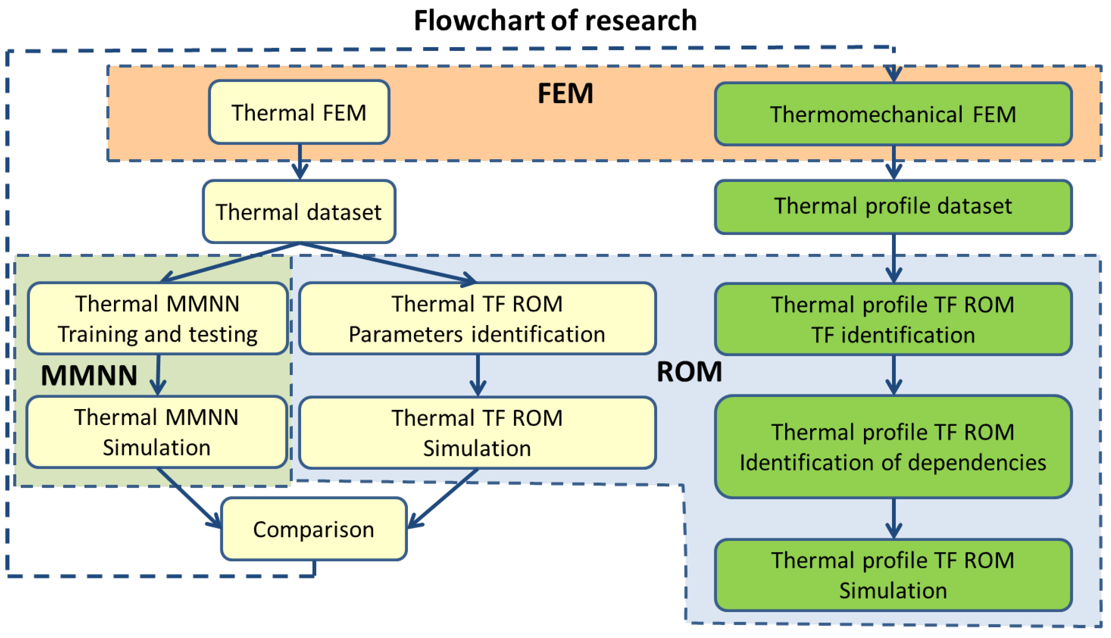
Figure 1 presents a flowchart of research connected with the development, study, identification, testing, verification, and simulation of thermal and thermomechanical models presented in this paper. There are three kinds of models: Finite Element Models (FEM), MetaModel based on Neural Network (MMNN), and Reduced-Order Models (ROM) based on Transfer Functions (TF—TF ROM). Blocks colored in yellow present thermal models, those colored in green present thermomechanical models, and models of thermal profile, roll, and sheet convexity. Thermal models, analytical and semianalytical solutions, FEM, MMNN, and TF ROM are considered in detail in Section 3. The thermal model allows us to obtain the temperature distribution, but does not solve the titled problem of thermal profile. However, thermal models allowed us to compare two proposed approaches, MMNN and TF ROM, and to choose the kind of model more suitable for the thermal profile.

The approach accepted for thermal MMNN is similar to the spatial discrete method used for partial differential equations (for example, finite difference method with an explicit calculation scheme). As can be seen in Section 3.3, every node takes information about the current and previous value of itself and neighboring nodes. TF ROM applies ordinary differential equations of the first, second, or higher order for every node without consideration of neighboring nodes, independently of them.

Section 4 is devoted to the analysis of these two approaches. Firstly, several FEM simulations were performed, and a dataset was created. Then, the dataset was used for training and testing of MMNN and identification of parameters of transfer functions. Finally, MMNN and TF ROM were compared, and TF ROM was chosen for further study thermal profile model. The arguments used are as follows. A network with nodes used MMNN for the considered problem requires at least 20 different NNs, and the choice of them is untrivial. The time of training the whole network with hundreds of nodes is very time-consuming. Thus, the approach was considered inappropriate, a dead-end, and of academic interest only. On the other hand, identification of the transfer function for the node is fast, simple, and independent of the other nodes of the modeled space. That is one of the causes of the choice of TF ROM, instead of MMNN ROM.

Section 5 presents the thermal profile model: FEM and TF ROM. For this problem, a recurrent neural network can likely be studied along with TF ROM. Identification, verification, and simulations of TF ROM and dependences on process conditions, material properties, and roll parameters are presented in Section 6.

3. Thermal Models

Thermal models can be classified as empiric, analytical, semi-analytical, numerical, and ROMs (or metamodels). Empirical models are not considered here due to their low usability.

3.1. Analytical and Semianalytical Solutions

Analytical models or solutions are based on a physical model but are limited to simple geometry, stationary states, and constant conditions. For more complex tasks, they use Green functions. Problems of one-dimensional linear symmetric and axisymmetric problems are described by the following equations:

$${\displaystyle \frac{\lambda }{\rho c_p}}{\displaystyle \frac{{\partial }^2\vartheta }{\partial x^2}}={\displaystyle \frac{\partial \vartheta }{\partial t}}$$

(1)

$${\displaystyle \frac{\lambda }{\rho c_p}}\left({\displaystyle \frac{{\partial }^2\vartheta }{\partial r^2}}+{\displaystyle \frac{1}{r}}{\displaystyle \frac{\partial \vartheta }{\partial r}}\right)={\displaystyle \frac{\partial \vartheta }{\partial t}}$$

(2)

with initial and boundary conditions, for example, for an axisymmetric problem:

$$\vartheta \left(r\right)=0$$

(3)

$${\displaystyle \frac{\partial \vartheta \left(0,t\right)}{\partial r}}=0\forall t\ge 0$$

(4)

$${\displaystyle \frac{\partial \vartheta \left(R,t\right)}{\partial r}}=-{\displaystyle \frac{\alpha }{\lambda }}\vartheta \left(R,t\right) \forall t>0;$$

(5)

where ϑ—excess ambient temperature, x—linear coordinate, r—coordinate along the roll radius, t—time, λ—heat conduction coefficient, ρ—material density, c_p—specific heat capacity, α—heat transfer coefficient, and R—roll radius.

A solution of Equation (1) at time t has the following form:

$$\vartheta \left(x,t+∆t\right)=\sum _{n=1}^{\infty }\left[{\displaystyle \frac{{\beta }_n\cos \left({\beta }_{n}x\right)}{{\beta }_n+\sin {\beta }_n\cos {\beta }_n}}exp\left(-{\beta }_n^2{\displaystyle \frac{4\lambda \mathsf{\Delta }t}{\rho c_p{h}^2}}\right){\int }_0^1\vartheta \left(x,t\right)\cos {\beta }_{n}xdx\right]$$

(6)

A coefficient β_n in (6) should be determined from the characteristic equation of a given relationship:

$$\mathit{cot}\beta ={\displaystyle \frac{2\beta \lambda }{\alpha h}}$$

(7)

where h—length of the analyzed domain.

Calculation time and accuracy with a semi-analytical solution depend on several parameters in (6). They are n, i.e., the number of first terms of a series that approximates the temperature, n_n—the number of nodes that affect the precision of calculating the integral in the equation, and Δt—the time step. The rational choice of these parameters makes the semi-analytical solution more efficient than most numerical solutions.

The analytical solution of the axisymmetric problem (2)–(5) can be presented as follows:

$$\vartheta \left({\displaystyle \frac{r}{R}},t\right)=\sum _{n=1}^{\infty }{A}_n{J}_0\left({\displaystyle \frac{{\mu }_{n}r}{R}}\right)exp\left(-{\mu }_n^2\mathrm{F}\mathrm{o}\right)$$

(8)

where $\mathrm{F}\mathrm{o}={\displaystyle \frac{\lambda t}{\rho c_p{R}^2}}$—Fourier number, μ_n—roots of the characteristic equation:

$${\displaystyle \frac{J_0\left(\mu \right)}{J_1\left(\mu \right)}}={\displaystyle \frac{\mu }{Bi}}$$

(9)

where J₀ and J₁—Bessel functions of first-type zero- and second-order, $\mathrm{B}\mathrm{i}={\displaystyle \frac{\alpha R}{\lambda }}$—Biot number, A_n—factors calculated from the following:

$$A_n={\displaystyle \frac{2Bi}{\left({\mu }_n^2+{Bi}^2\right)J_0\left({\mu }_n\right)}}$$

(10)

Both solutions, in general, can be presented as a sum of exponents, and these properties will be used in the thermal and thermal profile models presented in the latter section:

$$\vartheta \left(t\right)={\theta }_0\left[1-\sum _{n=1}^{\infty }{k}_{n}exp\left(-{\displaystyle \frac{t}{T_n}}\right)\right]$$

(11)

where k_n—gain factor, T_n—time constant, and J₀—input temperature.

Analytical and semi-analytical solutions are efficient for simple one-dimensional problems, but the thermal problem for the rolls of rolling mills cannot be reduced to one-dimensional problems.

3.2. Finite Element Model

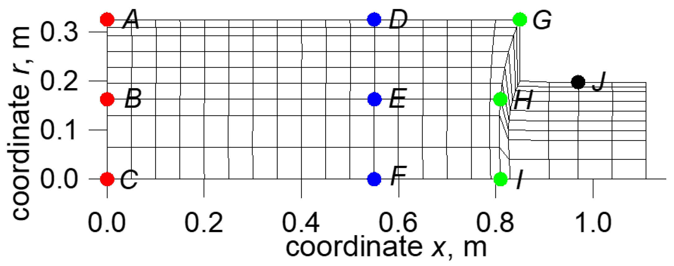
Heat conduction and then thermal expansion of the rolls can be presented as a two-dimensional axisymmetric problem. Due to symmetry, a quarter of the roll was modeled. A typical solution can be obtained with the use of the finite element method (FEM). Figure 2 presents the coarse mesh of the FEM model with several control points marked with the letters A–J (the color of the points means nothing).

The nonstationary thermal problem leads to a set of equations:

$$\mathbf{H}\mathbf{t}+\mathbf{C}{\displaystyle \frac{\partial \mathit{T}}{\partial t}}+\mathbf{p}=0$$

(12)

where T—vector of nodal temperatures. The matrices H and C and the vector p are defined as follows:

$$\mathbf{H}=\underset{V}{\int }\left[{\lambda }_x{\displaystyle \frac{\partial {\mathit{N}}^T}{\partial x}}{\displaystyle \frac{\partial \mathit{N}}{\partial x}}+{\lambda }_r{\displaystyle \frac{\partial {\mathit{N}}^T}{\partial r}}{\displaystyle \frac{\partial \mathit{N}}{\partial r}}\right]dV+\underset{S}{\int }\alpha {\mathit{N}}^T\mathit{N}dS$$

(13)

$$\mathbf{C}=\underset{V}{\int }{\mathit{N}}^T\rho c_p\mathit{N}dV$$

(14)

$$\mathbf{p}=-\underset{V}{\int }Q{\mathit{N}}^{T}dV-\underset{S}{\int }\left(\alpha T_0-q\right)\mathit{N} dS;$$

(15)

where N—matrix of shape functions. A further solution is based on the assumption of linear changes in nodal temperatures between t₀ and t₁ and the Galerkin integration scheme:

$$\left(2\mathbf{H}+{\displaystyle \frac{3}{\mathsf{\Delta }\mathbf{t}}}\mathbf{C}\right){\mathit{T}}_1+\left(2\mathbf{H}-{\displaystyle \frac{3}{\mathsf{\Delta }\mathbf{t}}}\mathbf{C}\right){\mathit{T}}_0+3\mathbf{p}=0$$

(16)

Equation (15) is a set of linear equations, which allows the calculation of the vector of the nodal temperatures T₁ after time Δt for the known temperatures T₀. The solution described above is used in the present work for the calculations of the temperature field in the rolls.

3.3. Metamodel with Neural Network

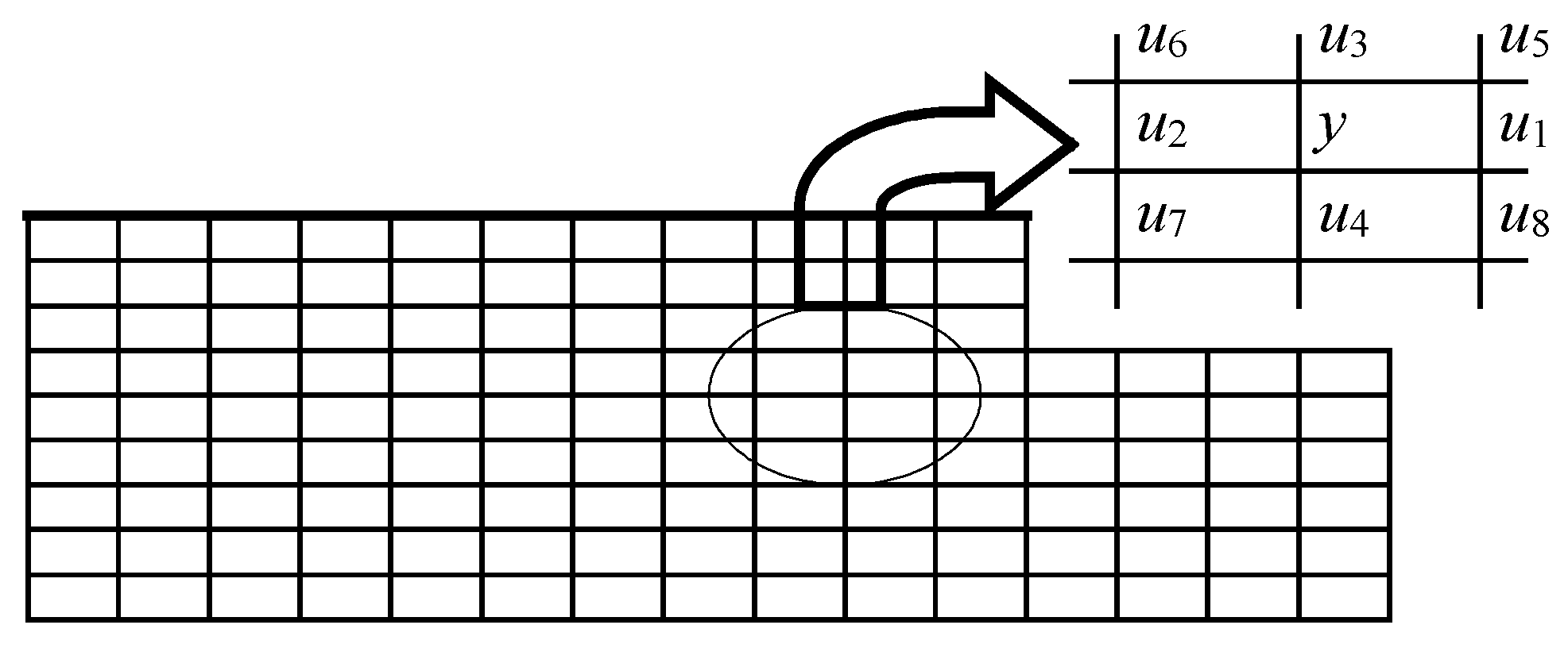
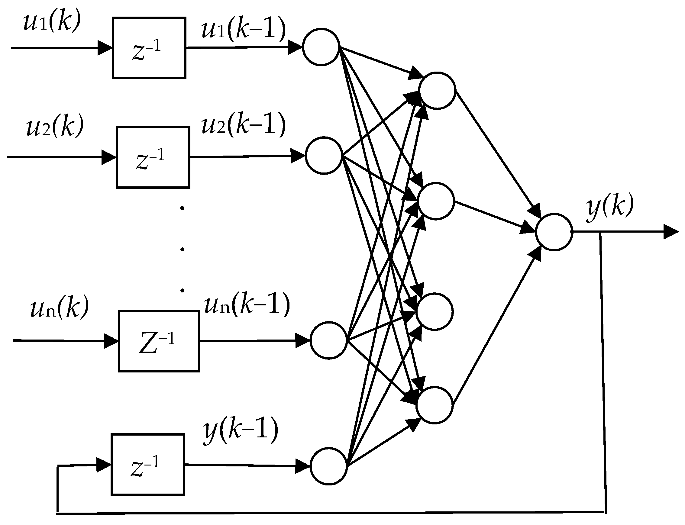
The author proposed to build such a structure of a thermal metamodel, in which a node of the FEM-like mesh is replaced by an artificial neural network (NN). This model can be treated in different ways, for example, as a finite difference method with an explicit calculation scheme and replacement of finite difference equations with a neural network, or as cellular automata with transition rules using a neural network, or as a modified Lattice Boltzmann method with a neural network. It was decided to name this model a metamodel with neural network (MMNN). Figure 3 presents schematically the mesh with node y, for which a neural network was built.

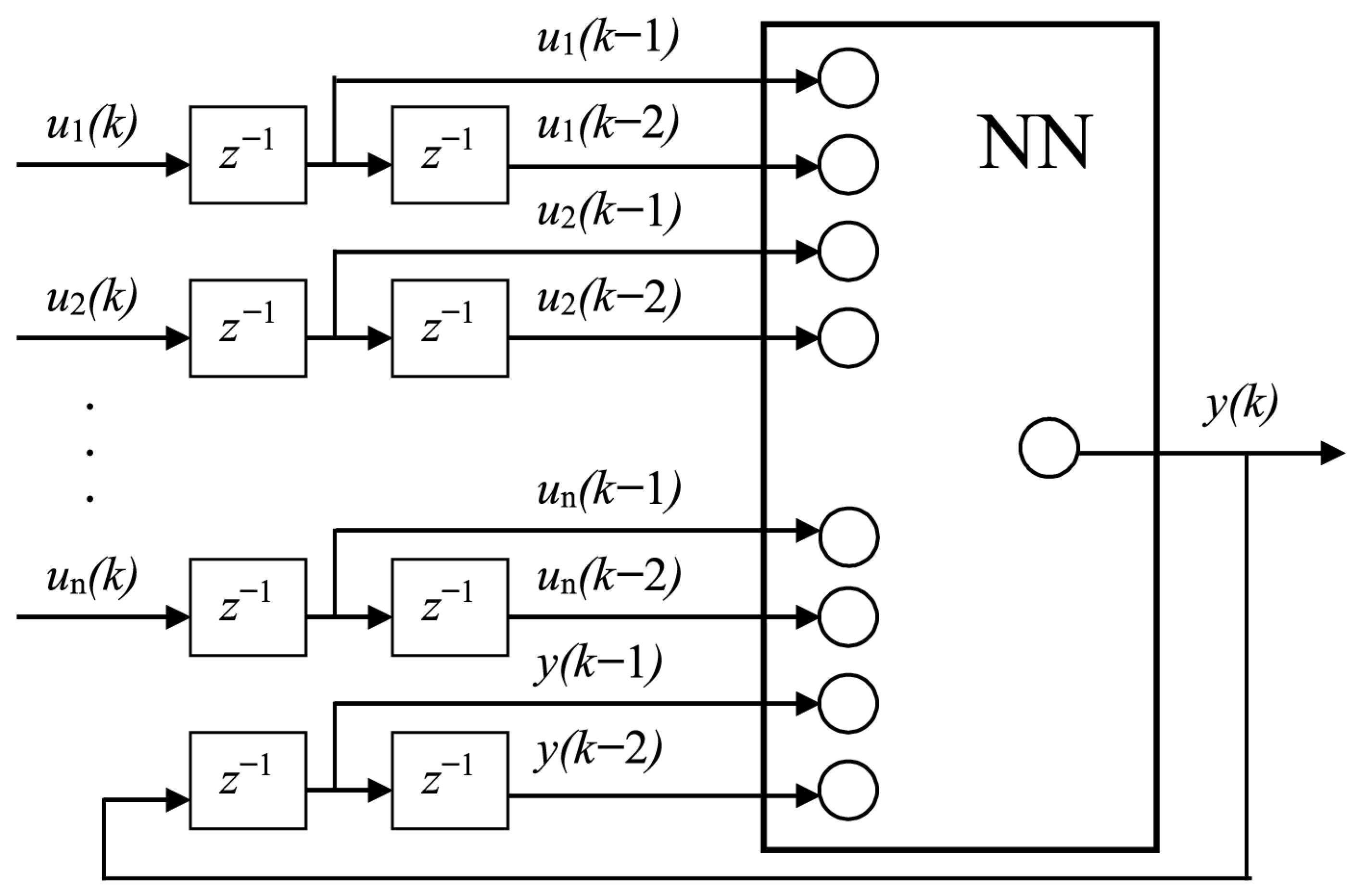
The basic structure of NN is shown in Figure 4. NN contains memory that can remember and take into account two previous states. This MMNN can be treated as ROM only partially and only in comparison with FEM. Explicit calculations in the proposed structure of MMNN can be easily parallelized, which additionally allows for a huge reduction in calculation time.

NNs with various configurations were tested, and the optimum configuration was determined. The NN can consist of four layers: input, output, and two hidden layers. Several variants of structures were studied. The number of previous states was determined first. The comparison of networks that account for one and two previous states did not show a visible difference. Further analysis has shown that the maximum number of inputs is 9. For the internal nodes, the inputs are the temperatures of all neighboring nodes and the node itself. Symmetry allows for a reduction in the number of inputs to 6. The relevant heat transfer coefficient, as well as the temperature of the hot plate and the cooling medium (water or air), are the additional inputs for the surface nodes. The number of neurons in the hidden layer was also adjusted as a result of training and testing.

3.4. Thermal ROM Based on the Transfer Functions

The general analytical solution (11) can be transformed into the form of a transfer function G(s) by applying an integral Laplace transform (or Laplace–Carson transform). Then, the solution can be presented as follows:

$$G\left(s\right)=\sum _{n=1}^{\infty }{\displaystyle \frac{k_n}{T_{n}s+1}}\approx \sum _{n=1}^N{\displaystyle \frac{k_n}{T_{n}s+1}}$$

(17)

Since the solution should not theoretically depend on the selected method, it can be said that analytical and numerical methods should give the same results. Thus, it can be stated that the results that cannot be obtained by analytical methods, but which can be obtained by numerical methods (e.g., FEM), can be presented in the same form, i.e., in the form of a transfer function.

The accuracy of solutions (11) and (17) depends on the order of the solution N (the number of components of the sum or terms of the series). The order of solution N, the gain factors k_n, and the time constants T_n can be found from the numerical solution.

4. Results of Thermal Model Simulations

This section contains results of FEM simulations, MMNN training, and verification.

4.1. Results of Thermal FEM Simulation

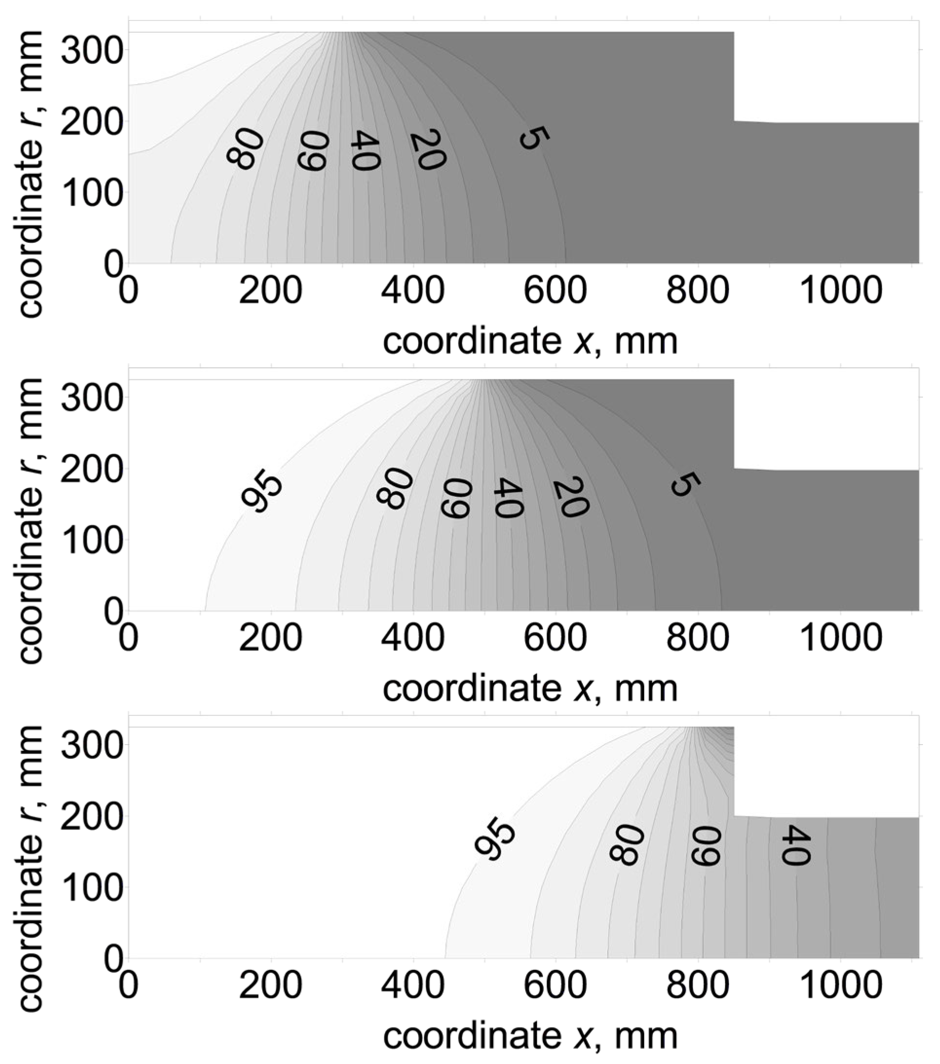
The results of the FEM simulation are presented in two forms: a temperature distribution at a fixed time and temperature changes at representative points. Figure 5 presents the temperature distribution in the roll after rolling strips of various widths. The rolling process was simulated until the temperature distribution reached a steady state. The results of the simulations of the widths of the rolling strip are presented in Figure 5: 600, 1000, and 1600 mm. The distributions for all three cases are similar in relation to the edge of the strip; some differences occur in the center of the roll for the narrow strip and at the edge of the roll for the wide strip. It can be said that the temperature field around the edge of the strip is independent of the width of the strip. For a strip width greater than 800 mm, the temperature distribution in the center of the roll length remains the same. When the width exceeds 1200 mm, changes appear in the neck of the roll. Parameters such as the heat transfer coefficient α, conductivity λ, and roll diameter D do not affect the shape of the steady state of the temperature distribution.

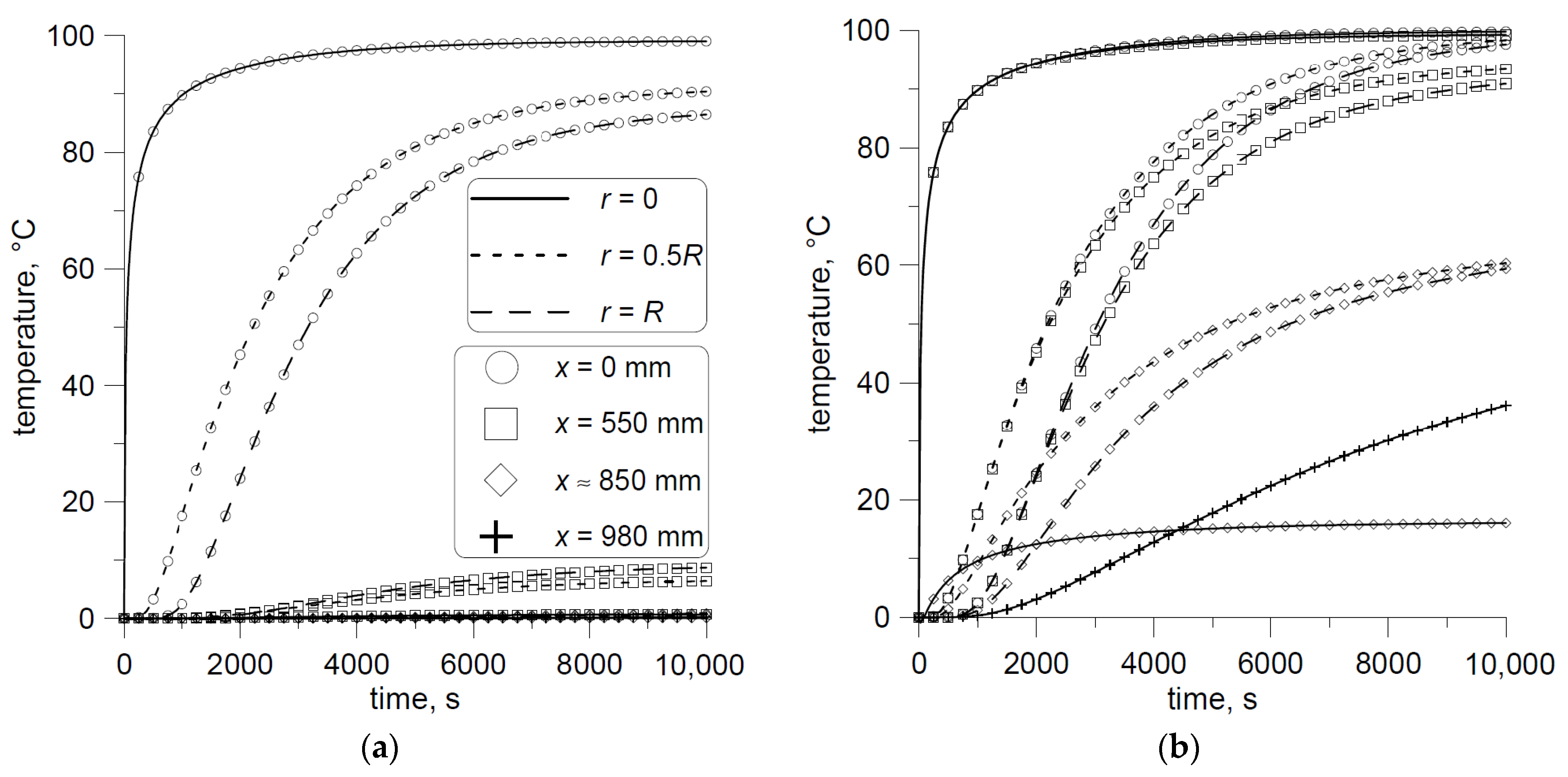
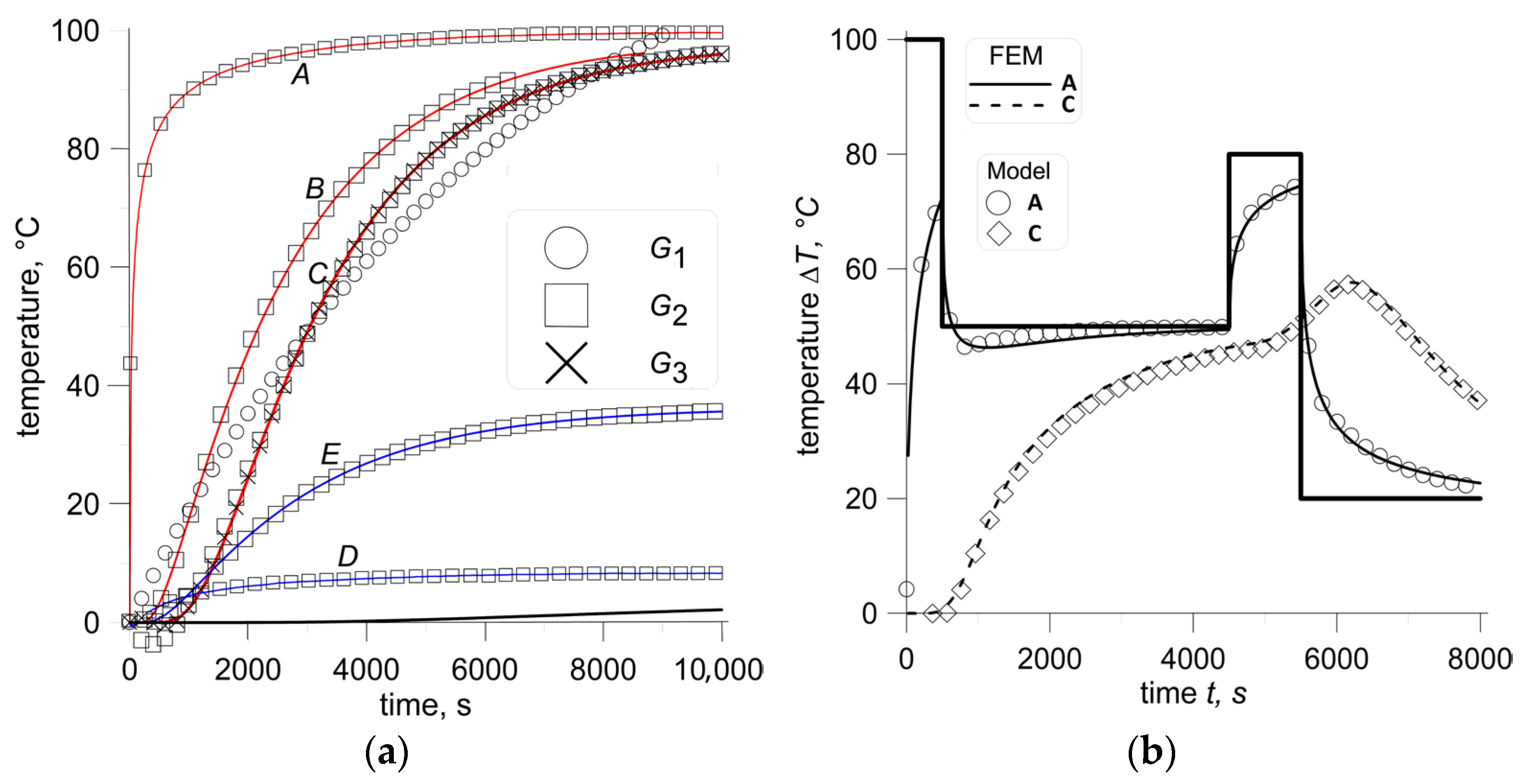
Changes in representative points A–J (Figure 1) were monitored during the simulation of the process with a step change in the boundary condition on the surface. A step change in surface temperature was 100 °C. The calculated temperature changes for two widths of the strip are shown in Figure 6. The coordinates r and x of the representative points are shown. The differences in the transient processes for various points are clearly seen in Figure 6. The delay in response increases with increasing distance from the surface and outside the edge of the strip. Analysis of the results for various widths shows the similarity of the temperature changes related to the edge of the strip. It can be concluded that not only static characteristics but also dynamic ones, when related to the edge of the strip, show insensitivity to the strip width.

Unlike the static characteristic, the dynamic is sensitive to the heat transfer coefficient α, the conductivity λ, and the roll radius R. An increase in α, λ, or a decrease in R accelerates the temperature changes (these results are not presented in this paper). The influence of various parameters on the dynamic characteristic can be investigated by an analytical solution (8) assuming time constants:

$$T={\displaystyle \frac{t}{{\mu }_1^{2}Fo}}={\displaystyle \frac{R^2}{{a\mu }_1^2}}={\displaystyle \frac{R^2\rho c_p}{\lambda {\mu }_1^2}}$$

(18)

where t—time, Fo—Fourier number, μ₁—the first root of the characteristic Equation (9).

Parameters that control the Fourier number (a, λ, R, and l) directly influence the time constants T, while the influence of the parameter α, which controls the Biot number, is much weaker. An increase in Biot number involves a slight increase in roots μ and a decrease in the largest (main) time constant T. Since parameters such as conductivity λ and roll radius R control both Fourier and Biot numbers, their influence on the time constants T is slightly lower than that calculated from the Fourier number only.

4.2. Results of Training and Verification of MMNN

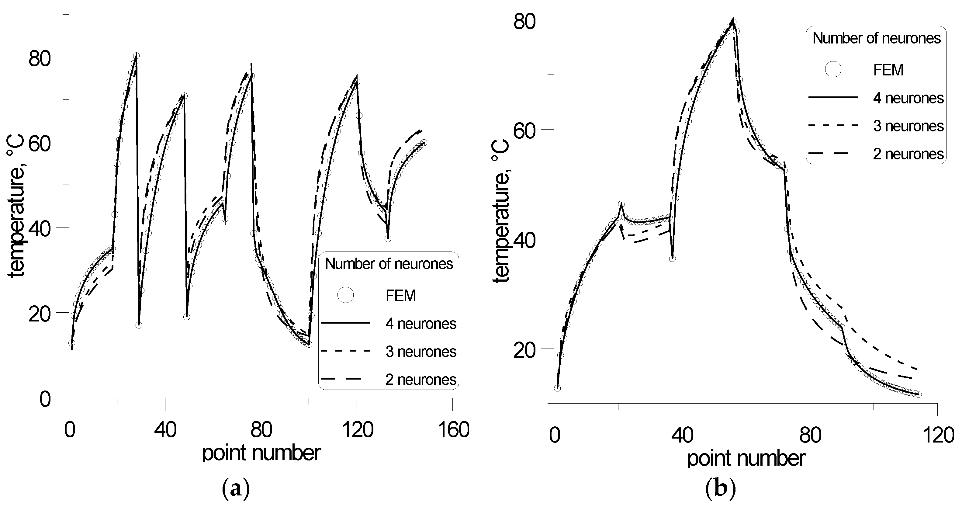
To obtain data for learning, testing, and verifying the network, several FEM calculations were carried out, containing several heating and cooling cycles. In these processes, the temperatures, the width of the strip, the heat transfer coefficient, the conductivity, the roll radius R, and other parameters were varied. Some cycles were selected for teaching, others for testing the network; finally, one of the processes was left for verification. The results of the NN testing and verification for one node are shown in Figure 7.

In Figure 7, it is seen that two neurons in the hidden layer do not give good results. Three hidden neurons give good training results, but testing still remains unsatisfactory. Four hidden neurons give good results for both datasets. However, signs of overtraining were observed for this network. An increase in the number of hidden neurons to 5 leads to larger differences in the accuracy obtained for training, testing, and verification.

The typical results of the training, testing, and verification of NN are shown in

Table 1. The results of training and testing various configurations of recurrent networks.

Dataset	Factor	2 Neurons	3 Neurons	4 Neurons (Case 1)	4 Neurons (Case 2)	4 Neurons (Case 3)
training	RMS error *	0.0229	0.0109	0.0073	0.0051	0.0031
	Good pct **	38.10	57.50	73.80	86.90	95.00
testing	RMS error	0.0215	0.0103	0.0181	0.0077	0.0450
	Good pct	28.40	66.20	35.80	80.40	9.50
verification	RMS error	0.0234	0.0081	0.0102	0.0048	0.0245
	Good pct	37.70	73.70	70.20	90.40	36.00

(* RMS error—root mean square error; ** Good pct—percentage of data points with root mean square error less than 0.01, [%]).

. Simple networks with two or three hidden neurons show similar accuracy in training, testing, and verifying datasets. The difference between these sets appears for the four hidden neurons. At the beginning of training (case 1), the difference in accuracy between the training and testing sets is clearly seen. When the network is properly trained (case 2), the accuracy of both sets increases and is closer to each other. Further training (case 3) leads to an increase in the accuracy of the training set and a decrease in the testing set. This phenomenon is characterized by overtraining of the network. Finally, the structure of the MMNN for the node contains NN with one hidden layer and four neurons in the hidden layer (Figure 8).

MMNN resented in this section was implemented on a GPU that allowed one to obtain a temperature distribution in a much shorter time than the online (real-time) control system requires. Each real-time step (20 s) is calculated in approximately 0.1 s. However, this model was not used in the roll calculations of the thermal profile due to the need to introduce a temperature distribution into the thermal expansion model. A different model described below was used for the thermal model of the thermal profile. So, the model described in this subsection has mainly an academic character and, for its implementation, requires too many FEM calculations and teaching of NNs.

4.3. Identification and Verification of Thermal ROM

As shown in Section 3.4, the temperature at an arbitrary point in the roll can be presented in the form (17). The temperature transient function or the response to the unit step function obtained from the FEM simulations is used to identify the ROM parameters (transfer functions), i.e., order N, gain factors k_n, and time constants T_n. MATLAB (version R2022b) Control Identification Tools were used here. Data for learning, testing, and verifying the network previously obtained with FEM simulations were also used for the identification of ROM parameters.

Figure 9 presents the result of the ROM compared to the results of the FEM simulations. Temperature changes are shown for representative points A, B, C, D, and E (see Figure 2). For representative point C (Figure 9), the results are plotted for three transfer functions of the first, second, and third orders, and for the other point, the transfer function of the second order only. The transfer function for point C with root mean square error is as follows:

$$G_{C1}={\displaystyle \frac{1.3254}{6412.6s+1}}; \chi =7.435 °\mathrm{C}$$

(19)

$$G_{C2}={\displaystyle \frac{4.034}{1801.7s+1}}-{\displaystyle \frac{3.059}{1245.6s+1}}; \chi =1.068 °\mathrm{C}$$

(20)

$$G_{C3}={\displaystyle \frac{2.188}{2063.3s+1}}-{\displaystyle \frac{1.851}{691.7s+1}}+{\displaystyle \frac{0.639}{363.4s+1}}; \chi =0.208 °\mathrm{C};$$

(21)

$$G_{C4}={\displaystyle \frac{2.016}{2149.2s+1}}-{\displaystyle \frac{2.235}{559.2s+1}}+{\displaystyle \frac{1.684}{309.5s+1}}-{\displaystyle \frac{0.485}{198.1s+1}}; \chi =0.0353 °\mathrm{C}.$$

(22)

The accuracy of the second-order transfer function of can be considered sufficient for most points (see the results for points A, B, D, and E in Figure 9), although for some points, the third-order transfer function of should be taken. The transfer functions for the other representative points are as follows:

$$G_{A2}={\displaystyle \frac{0.55}{68.8s+1}}+{\displaystyle \frac{0.45}{1015.8s+1}};$$

(23)

$$G_{B2}={\displaystyle \frac{1.45}{1699.3s+1}}-{\displaystyle \frac{0.45}{458.2s+1}};$$

(24)

$$G_{D2}={\displaystyle \frac{0.0465}{1750s+1}}+{\displaystyle \frac{0.0049}{207s+1}}$$

(25)

$$G_{E2}={\displaystyle \frac{0.561}{4635s+1}}-{\displaystyle \frac{0.235}{1898s+1}}.$$

(26)

The verification of the model consisted of modeling the process in which the thermal boundary condition was changed several times by step and comparing the modeling results of the two models. Temperature changes on the roll surface and the modeling results for representative points A and C are shown in Figure 9b), and show good agreement between the results of the two models.

The time of calculation for one real-time step (20 s) by the ROM presented in this section is below 0.01 s. However, this model (as well as MMNN) was not used in the calculations of the thermal profile of the roll due to the need to introduce a temperature distribution into the thermal expansion model.

5. Models of the Thermal Profile of the Roll

In this section, two models of the roll thermal profile are presented. The first model is the thermal expansion FEM model based on the data obtained from the thermal FEM model, although, in fact, the thermal and thermal expansion FEM models were then joined into one FEM model. The second model is the ROM based on the transfer functions.

5.1. Thermal Expansion FEM Model

The roll profile is calculated by a solution of linear stiffness equations for deformations caused by thermal expansion. The linear stiffness equation is the following:

$$\mathbf{K}\mathbf{d}=\mathbf{f}$$

(27)

where K—stiffness matrix, d—vector of nodal displacements, f—vector of forces.

The stiffness matrix K and the vector of forces f can be calculated as follows:

$$\mathbf{K}=\underset{V}{\int }{\mathit{B}}^T\mathit{C}\mathit{B}dV$$

(28)

$$\mathbf{f}=\underset{V}{\int }{\mathit{B}}^T{\displaystyle \frac{E\alpha \vartheta }{1-2\upsilon }}1dV$$

(29)

where B—matrix of derivatives of shape functions, C—constitutive matrix (Hook’s matrix), and f—vector of forces. E—Young modulus, ν—Poisson coefficient, and α—thermal expansion coefficient, 1 = {1,1,10}^T.

Then, the thermomechanical FE model contains two modules: the thermal FEM model (12)–(16), which calculates changes in temperature distribution during the process, and thermal expansion FEM (27)–(29), which calculates deformations based on temperature distribution. As a result, changes in displacement (deformation) of an arbitrary point are presented as transient functions, that is, time dependencies of displacement on the step changes in input variables (boundary conditions).

5.2. Thermal Profile ROM with Transfer Functions

The temperature distribution in the roll and the thermal expansion coefficient α are the main factors determining the thermal profile of the roll. Young’s modulus E and the Poisson coefficient ν, which significantly influence the value of thermal stresses, do not influence the roll profile. The influence of the thermal expansion coefficient α is linear. The smaller the distance to the point from the surface, the stronger and more localized the influence of its temperature on the roll diameter.

When the temperature distribution is known, the influence of the temperature of each node on the roll diameter and the surface profile can be determined (for example, by a thermal expansion FEM model). Thus, the roll profile can be calculated using an additivity rule. This can simplify the calculations of the roll thermal profile. However, the large number of nodes and the dependence of nodal temperatures on surface temperature and several process and material parameters significantly limit the task of determining nodal temperatures for different conditions.

Therefore, another approach was suggested. The profile of the roll surface can be presented as a combined influence of the temperature at single nodes. The nodal temperatures can be calculated using the transfer functions (17), which are the sum of simple transfer functions. Therefore, the profile of the roll surface can be presented with the use of transfer functions of appropriate order (or the number of simple transfer functions). Then, data for identification of transfer functions can be obtained from the FEM simulations, taking into account that the model of the profile of the roll surface does not require temperature distribution, and two FEM models are joined, and only the results of the following profile are needed for the ROM.

Therefore, the ROM of the thermal profile with transfer functions can be presented by (17) or as follows:

$$G_x={\displaystyle \frac{\mathsf{\Delta }{r}_x}{{\vartheta }_r\left(x\right)}}\approx \sum _{n=1}^N{\displaystyle \frac{k_n\left(x,R,b,\alpha ,a\dots \right)}{T_n\left(x,R,b,\alpha ,a\dots \right)s+1}}$$

(30)

The outputs Δr_x of (30) are the changes in the coordinate r (along the roll radius) of the points on the roll surface, which are defined by the coordinate x (along the roll axis). The input of (30) is the temperature distribution on the roll surface as a function of the coordinate x. The temperature of the surface of the rotated roll is calculated taking into account the heating with hot metal and the cooling with water and air. Gain factors and time constants are dependent on several parameters (coordinate x, roll radius R, width of rolling strip b, thermal diffusivity a, heat transfer coefficient α, etc.) and are independent of temperature. The determination of the order of the transfer function and the identification of the parameters of the dependences of the gain factors and time constants is the essence of the ROM identification.

6. Identification and Verification of Thermal Profile ROM

6.1. Identification of Dynamic Characteristic of the ROM

Identification of the thermal profile ROM was performed on the database created with FEM simulations for different conditions. This ROM was applied to different rolls for reverse and continuous mills with different roll sizes. In this paper, the roll with a diameter D = 650 mm and length l = 1700 mm is analyzed. The parameters of the model are varied in the following bounds:

• Roll diameter D = 615–685;
• Strip width b = 600–1600 mm;
• Thermal conductivity λ = 14–40 W/mK;
• Heat transfer coefficient a = 500–4000 W/m²K.

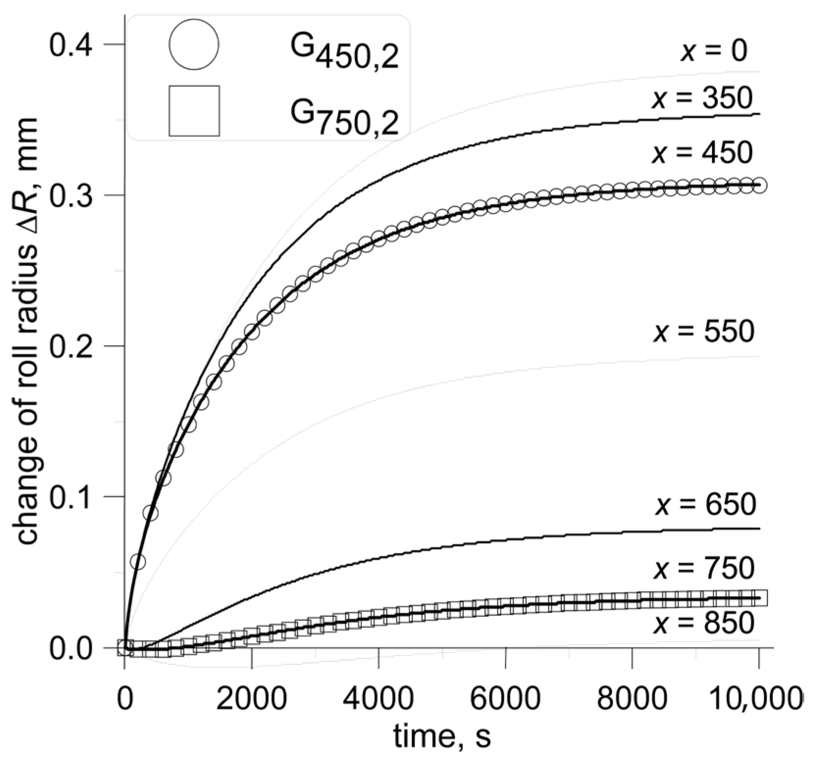
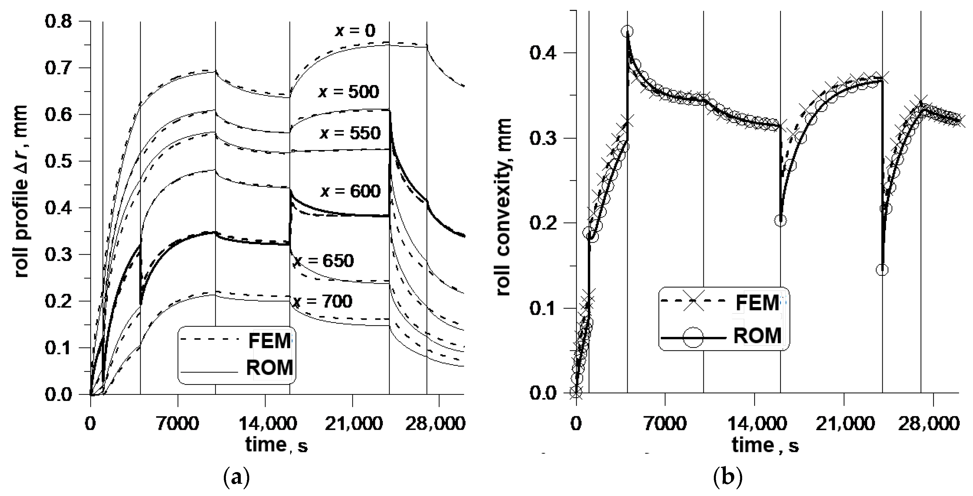
An example of FEM and ROM simulations is presented in Figure 10. It shows changes in the roll profile Δr for selected points on the roll surface. Coordinate x represents the distance between the point and the middle of the roll length. It is seen in this figure that changes in the roll profile depend on the location of the point.

The second-order transfer function was established to be satisfactory for an accurate prediction of changes in the thermal profile of the roll. The same results can be obtained by some modification of (17) or (30) as shown below:

$$G_x={\displaystyle \frac{\Delta r_x}{{\vartheta }_r\left(x\right)}}\approx {\displaystyle \frac{k_1}{T_{1}s+1}}+{\displaystyle \frac{k_2}{T_{2}s+1}}={\displaystyle \frac{k}{T_{1}s+1}}·{\displaystyle \frac{Ts+1}{T_{2}s+1}}$$

(31)

Four parameters are necessary to determine the transfer functions in both cases. These include the same time constants T₁ and T₂ in both cases and the coefficient k and the time constant T in the second case, instead of two coefficients k₁ and k₂ in the first case. The coefficient k(x) can be treated as a static characteristics that directly show the shape of the roll surface. The roll profile always tends to the profile determined by the coefficient k. The time constants T₁, T₂, and T are the parameters of the dynamic characteristics that show how long the transient process is.

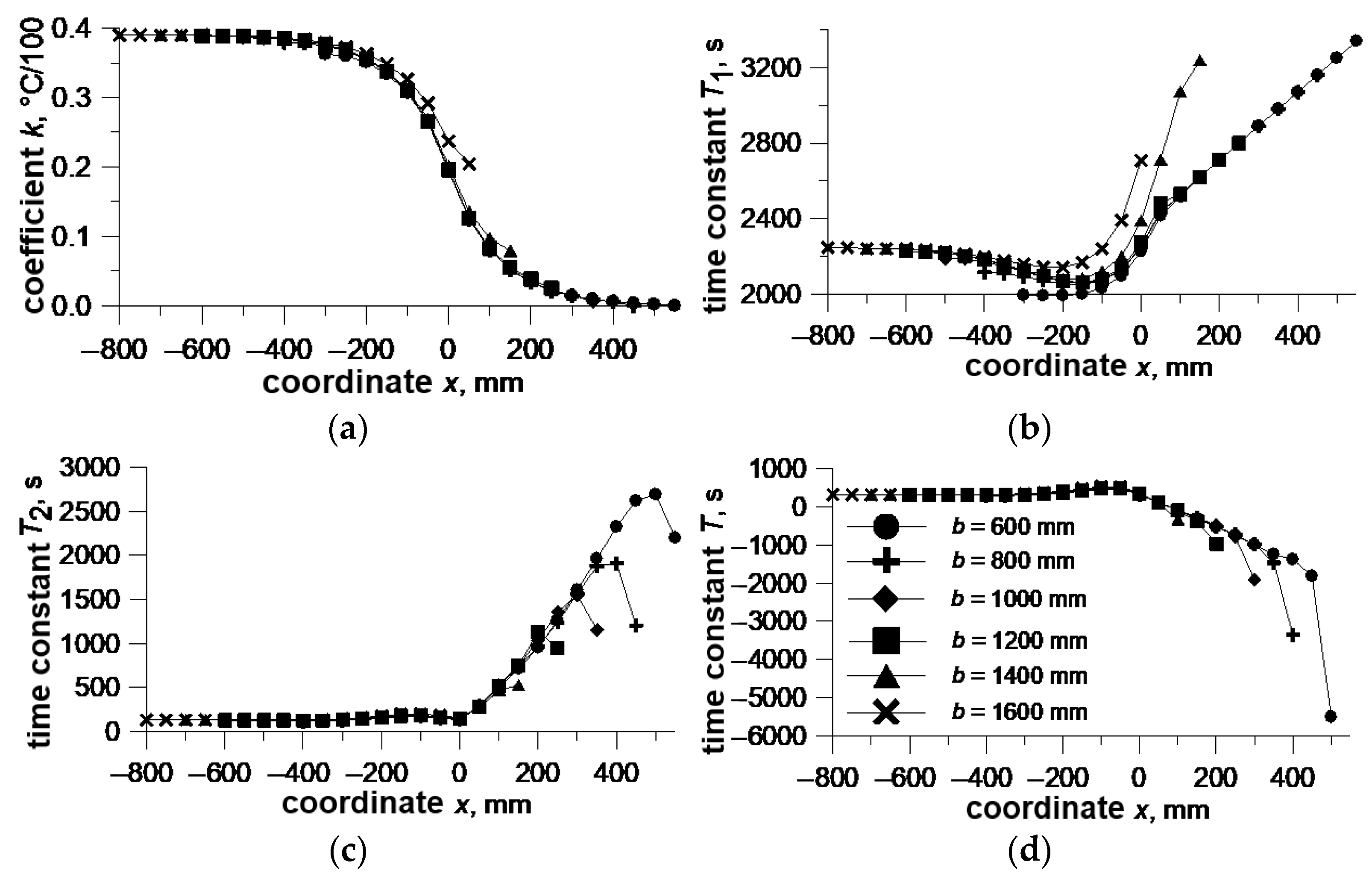
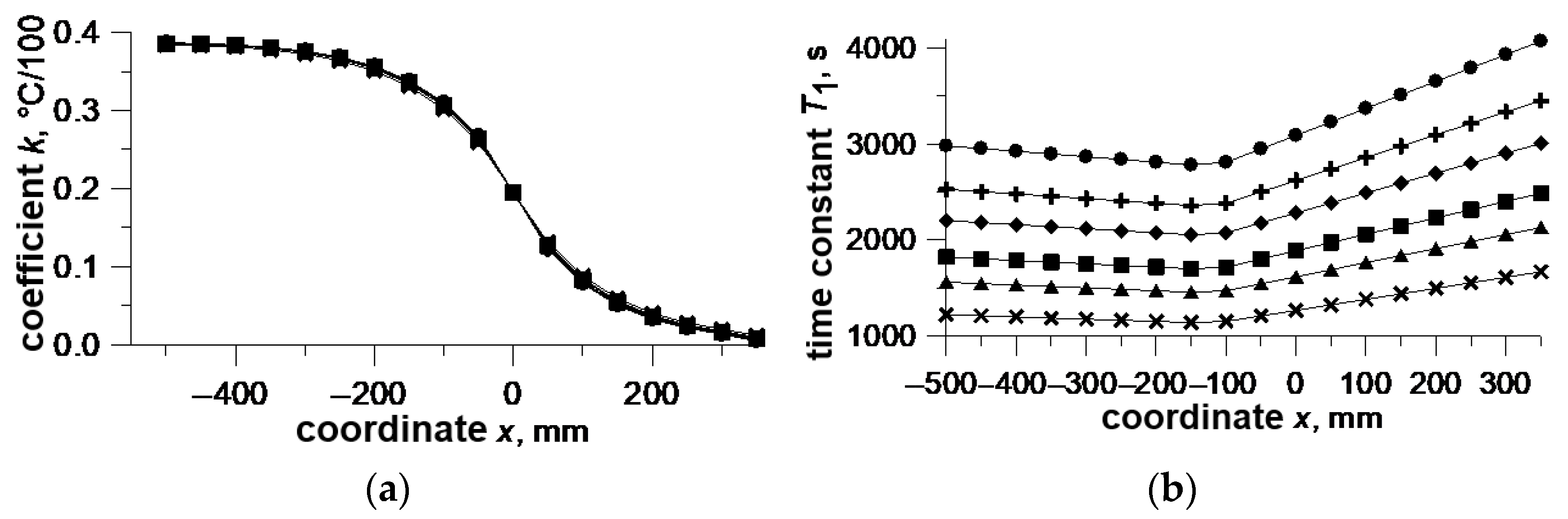
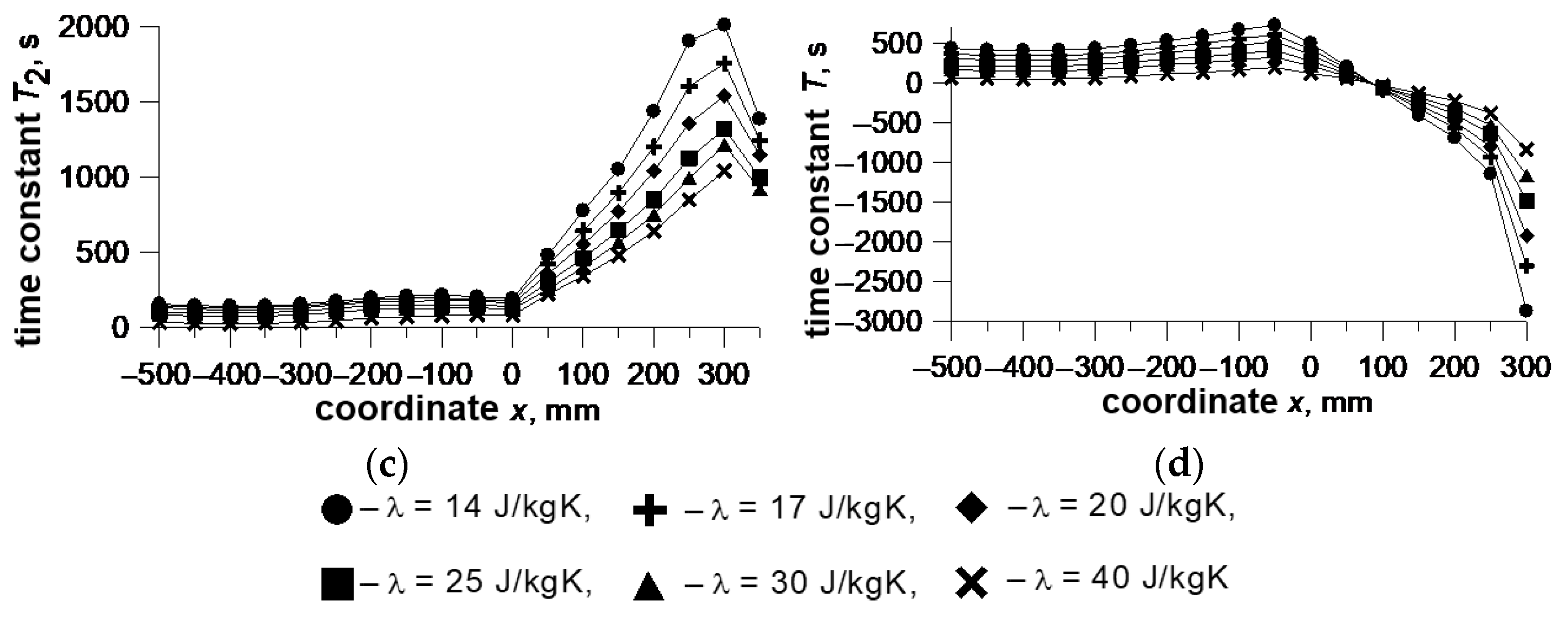
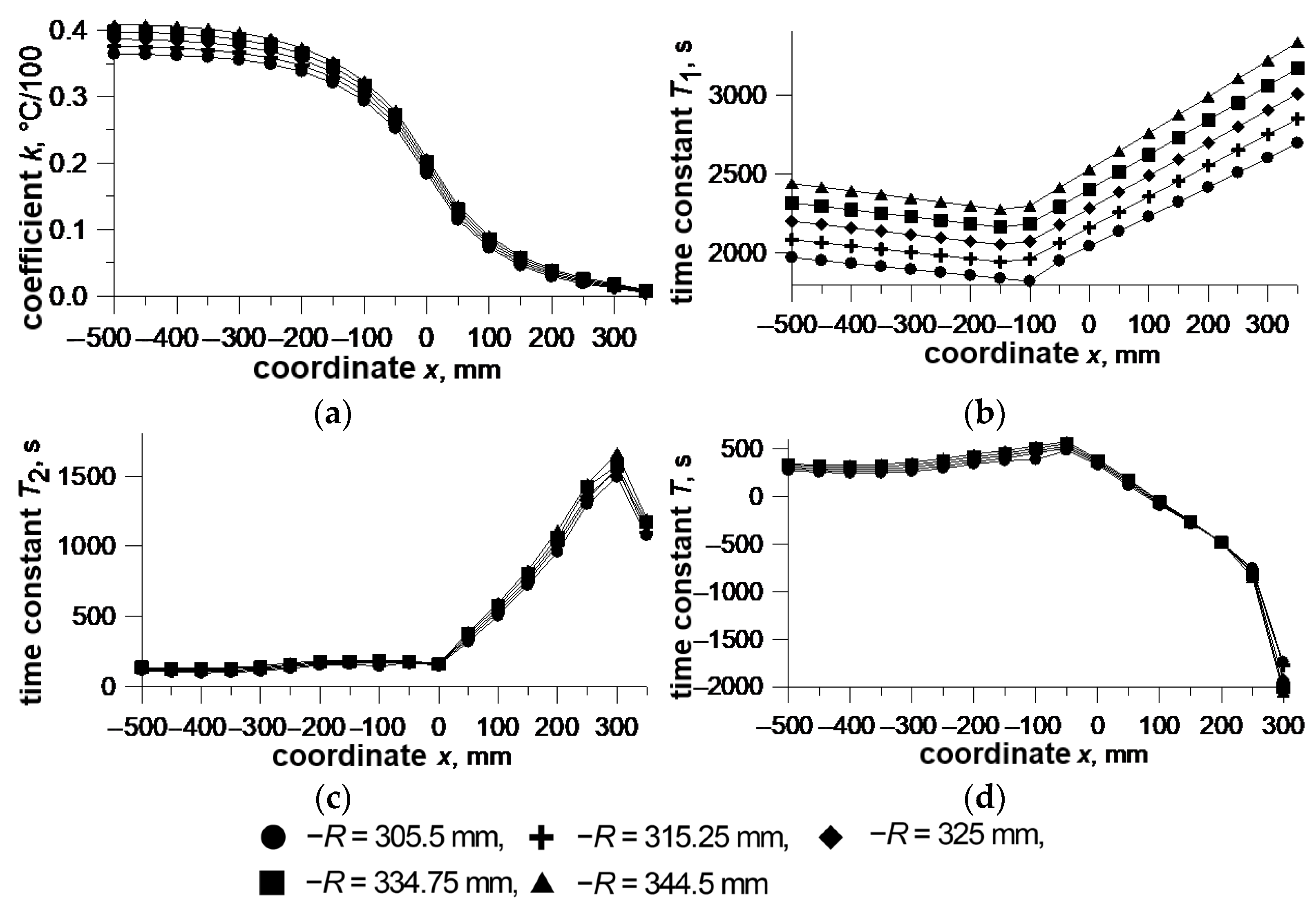
Some results of the identification of parameter functions k(x,R,b,α,a…), T₁(x,R,b,α,a…), T₂(x,R,b,α,a…), and T(x,R,b,α,a…) are presented in Figure 11, Figure 12 and Figure 13. The coordinate x = 0 refers to the edge of the strip that almost eliminates the effect of a different strip width.

An analysis of the changes in the parameters shows that the coefficient k is the least sensitive to most parameters. Some time constants are strongly dependent on some parameters, and others are almost independent.

6.2. Roll Convexity

The roll diameter, conductivity, and heat transfer coefficients are the parameters that do not change during one roll campaign or only change slightly. The width of the strip is the main variable in the process. In the coordinate system connected to the edge of the strip, the coefficient k is almost constant. Thus, it can be assumed that this coefficient does not change in the middle of the roll and at its edge. The largest changes in this coefficient are observed in the previous and next locations of the edge of the strip. An increase in width involves an increase in high-temperature contact and an additional roll expansion. On the contrary, a decrease in width results in a decrease in high-temperature contact and a decrease in roll expansion. In this case, the roll profile tends to that determined by the coefficient k, but the time constants evaluated from previous relationships cannot be applied. This is related to the fact that the relationships that describe time constants can be divided into two parts. The first part deals with the contact zone and influences the dynamic characteristics in this zone. The second part deals with the area beyond the contact zone and accounts for the mutual influence of one zone on another.

Roll convexity is a variable that is used in the real-time control system at a higher level to calculate the convexity of the rolling strip and in the subsystem controlling the flatness of the strip. Roll convexity is determined by roll diameters at two points: in the middle of the roll and at the edge of the strip. Then, only these two values have to be calculated. The thermal expansion in the middle of the roll and the time constants for this point are almost insensitive to changes in width. The roll expansion at the edge is almost constant. However, a change in the width of the strip leads to a rapid change in the coefficient k for the edge of the strip, while the time constants do not change. This means that the dynamic model of roll convexity has a variable characteristic, which is a dependence of k on the coordinate x. This characteristic is needed for the calculation of the roll profile at the edge of the strip caused by the change in width. Thus, dynamic models should contain two terms with constant input and an artificially changing output signal. The transient process due to the change in the width comprises two segments of the exponential function (time constants T₂ and T are small compared to T₁) with a constant asymptote and small steps in the direction dependent on the direction of the change in the strip width.

The results of the calculations for the whole roll campaign, which was designed for ROM testing, are shown in Figure 14. These results were obtained from the FEM model and ROM with the artificial NN for the parameter functions and with a discretization of the strip width and the average values of temperature and strip thickness. The changes in the roll profile are shown for selected points on the roll surface. Figure 14a shows that FEM and ROM give similar results for the roll profile. When the width of the strip changes, there is a rapid change in the roll profile. The change in strip thickness can also be seen in Figure 14a for a time near 1000 and 2700 s when the width of the strip does not change. The reduction leads to a change in the time of contact, and consequently to a change in the average temperature and the heat transfer coefficient. Also, the roll convexities calculated by the two models are close to each other.

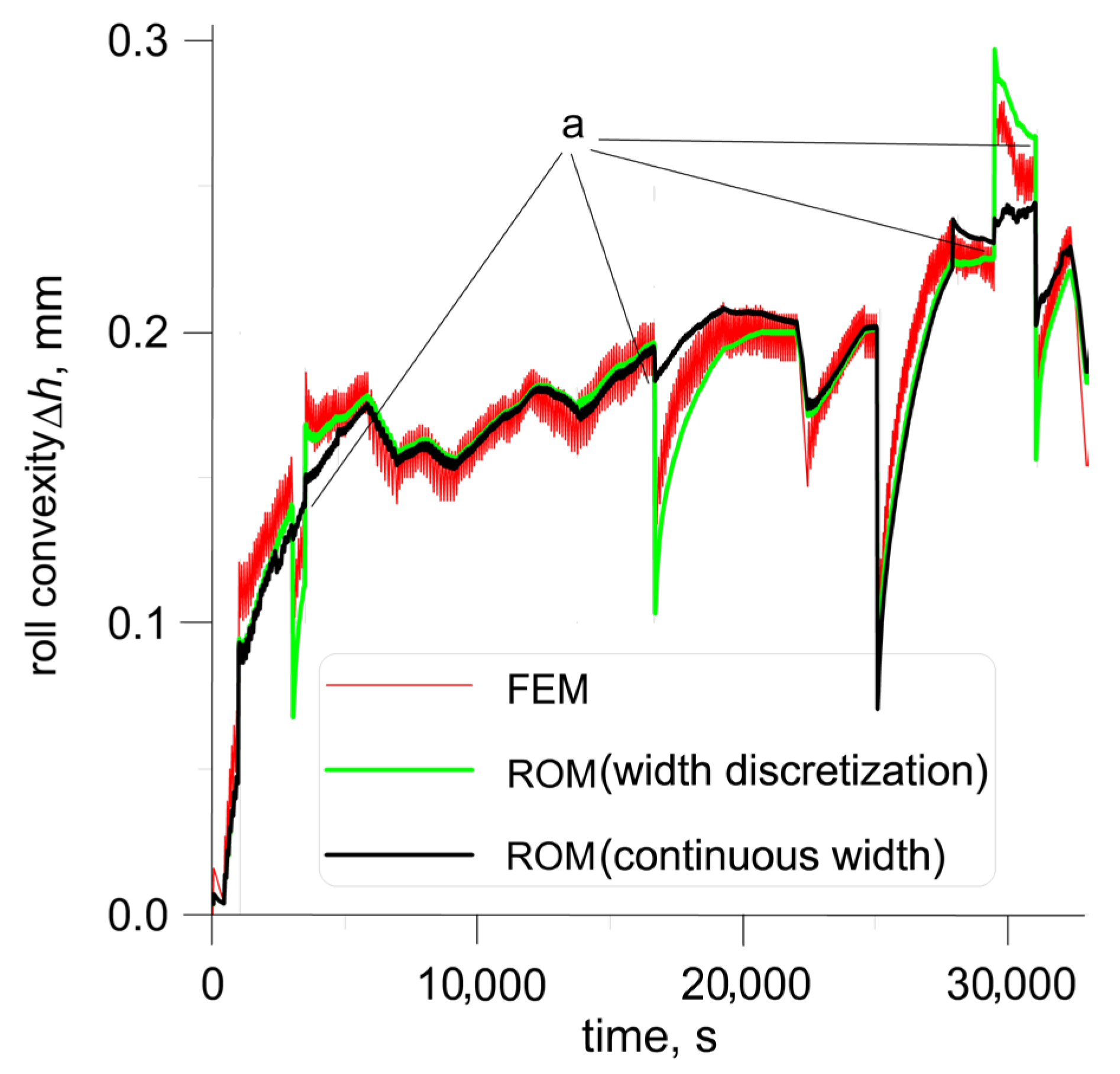
Other results are presented in Figure 14. Here, data from the real roll campaign (over 9 h, 683 strips) were applied for calculations by the FEM model and two variants of ROM, with discretization of the strip width and without such a discretization. The horizontal size of the finite element was 100 mm, and the same discretization level was applied for the first ROM. The strip width was rounded, and it introduces a round-off error. Then, the FEM model and the first variant of ROM have the same round-off error, while the second variant of ROM is free of this error. The discretization (rounding) of the width of the strip produces unjustified jumps in the roll profile, marked by the letter ‘a’ in Figure 15. This is the case, small changes in the strip width caused a change in the rounded width in the model by the length of the finite element (100 mm). Comparison of the FEM model and discrete ROM shows good agreement in changes in roll convexity, but the results have additional round-off error, whereas the continuous ROM shows somewhat different results, but they are more accurate because they are free of this round-off error.

Calculations of the whole campaign by the FEM model last several hours, while those by ROM last several seconds. A real-time step used in the real-time system for updating roll convexity is equal to 20 s; this real-time step is simulated by ROM less than 0.01 s. Calculations of the entire campaign by the ROM last less than 20 s. The ratio of the real process time to the ROM simulation time is approximately 1650.

7. Conclusions

The paper presents developed ROMs based on the transfer functions for calculating temperature distribution, thermal profile of the roll (shape of the roll surface), and roll convexity. Novelty of the proposed ROM is the application of transfer functions for a fast calculation of the shape of the roll surface, the convexity of the roll surface, and the rolling sheet (strip). The ROM of the convexity of the rolling sheet can be applied to the real-time control of the convexity and flatness of the final rolling product. Elements of the ROM were implemented into the control system of two rolling mills. Analysis of the results of the calculations confirms the high efficiency of the proposed ROMs and their feasibility for application in real-time control systems. ROM predicts the thermal profile of the roll with reasonably good accuracy in a very short time. This model, combined with the other models (which calculate roll bending and roll wear), allows predictions of the plate, sheet, and strip profile and flatness during rolling. The results of the calculations presented in the paper confirm the good predictive capabilities of the model. Very short computing times permit an application of this model in real-time control systems. It is planned to connect the FE model with the identification of ROM parameters in one computing block, which will allow the input of the basic parameters of the roll, its material, and possible rolling conditions, and the receipt of the complete ready dependencies of the ROM parameters at the output, which can be feasible for direct application of the ROM.