Enhancing Medium-Term Load Forecasting Accuracy in Post-Pandemic Tropical Regions: A Comparative Analysis of Polynomial Regression, Split Polynomial Regression, and LSTM Networks

Abstract

This research focuses on medium-term load forecasting in a tropical region post-pandemic. This study presents one of the first attempts to analyze medium-term forecasting using half-hourly resolution in the Java-Bali power system post-COVID-19 period. The dataset comprises load measurements recorded every 30 min (48 data points per day) from 2014 to 2022. Three distinct methods, namely polynomial regression, split polynomial regression, and Long Short-Term Memory (LSTM) networks, were employed and compared to predict the electricity load demand. The analysis found that LSTM outperformed the other methods, exhibiting the lowest error rates with Mean Absolute Percentage Error (MAPE) at 3.86% and Root Mean Squared Error (RMSE) at 1247.93. Additionally, a consistent observation emerged, showing that all methods performed better in predicting load demand during nighttime hours (6 p.m. to 6 a.m.). The hypothesis is that data stability during nighttime, with fewer significant fluctuations, contributed to the improved prediction accuracy. These findings provide valuable insights for improving load forecasting in the post-pandemic tropical region and offer opportunities for enhancing power grid efficiency and reliability.

1. Introduction

An accurate load forecasting plays a crucial role in the efficiency and reliability of power plant operations. The ability to predict future electricity demand with precision allows power plant operators to optimize generation schedules, plan maintenance activities, and allocate resources effectively. Furthermore, load forecasting is vital for grid operators to ensure the stability and security of the power grid, as it enables them to anticipate demand fluctuations and make timely adjustments to meet consumer needs.

Load forecasting can be divided into three types based on the forecast period: short-term load forecasting, medium-term load forecasting (MTLF) [1,2,3], and long-term load forecasting [4]. Short-term forecasting predicts demand for the upcoming day to weeks ahead. Usually, it aims to optimize the electricity supply in a system by paying attention to system reliability and economic aspects. Medium-term load forecasting predicts one month to one year ahead, aims to plan fuel reserves and other primary energy, and confirms unit commitments. The results of this forecast are generally in the form of peak load and average daily consumption. Lastly, the long-term load forecasting estimates load for annual to ten-year periods, used for expanding the construction of new power plants and transmission systems used for power evacuation.

However, the COVID-19 pandemic introduced unexpected and substantial shifts in electricity consumption behavior, particularly in tropical regions such as Indonesia. Sudden changes in demand patterns, irregularities during lockdown periods, and changes in industrial and residential usage significantly disrupted traditional load curves. These anomalies pose unique challenges for existing forecasting models, which often struggle to capture abrupt deviations or adjust dynamically to post-pandemic recovery phases.

In recent years, significant advancements have been made in load prediction techniques, driven by the demand for reliable electricity supply, integrating renewable energy sources, and developing smart grid technologies. Some of the methods are linear regression [4,5], autoregressive methods [6], and artificial neural networks [7]. Studies such as that by Bouktif et al. [8] have demonstrated the efficacy of combining deep learning LSTM-RNN models with metaheuristics for electric load forecasting, significantly improving accuracy [6]. Similarly, Masood et al. [9] proposed a clustering-based Seq2Seq LSTM model tailored for household electricity forecasting, which proves essential in the context of distributed energy systems and demand response [7]. Sun et al. [10] introduced the integration of time-series decomposition with kernel-based extreme learning machines for more accurate demand-side forecasting. Among the various methodologies employed for load forecasting, this paper focuses on three distinct approaches: polynomial regression, split polynomial regression, and neural networks in the form of Long Short-Term Memory (LSTM). These techniques represent different paradigms in load forecasting, offering unique advantages and considerations. LSTM-based techniques, in particular, have shown superior performance for load prediction in spatially distributed systems, such as the integrated energy system model proposed by Jember et al. [11], which utilizes CNN-LSTM and multi-task learning for improved spatial load transferability.

MTLF has held significant importance as a crucial tool over the past decade, primarily for scheduling repair and maintenance and economically optimizing energy systems, directly impacting reliability. The MTLF typically spans several months to one or two years, aiding in resource allocation and developing sub-structural elements within this mid-term. Additionally, mid-term forecasting enhances density management in transmission grids, thereby improving overall system productivity and optimizing consumer energy costs. Accurate MTLF offers businesses opportunities to enhance both distribution and transmission networks. Recent works by Yaprakdal and Arısoy [12] reinforce the importance of feature selection in multivariate time series to increase interpretability and forecasting quality.

The economic impact of MTLF on markets and distribution systems over the last two decades has been explored by Hamzaçebi et al. [13]. Today, MTLF is gaining attention in energy transactions, facilitating monthly or annual negotiations for energy buying and selling, aiding in developing production, transmission, and distribution contracts, and influencing generator vendors. Inaccurate forecasting can lead to supply inadequacies, affecting economic growth negatively or oversupplying, increasing production costs, ultimately borne by consumers. Therefore, precise MTLF contributes to a more competitive economic landscape [14].

The literature review reveals varying approaches and time horizons for MTLF among researchers. Some papers focused on a one-year horizon [10], while others conducted monthly forecasting [15], and Ref. [16] considered a multi-month horizon. Adedeji et al. [17] extensively studied the effect of weather on load prediction in MTLF, while Elkateb et al. [18] proposed an autonomous approach model based on load rates and meteorological data. Doveh et al. [19] introduced an Artificial Neural Network (ANN) model outperforming statistical techniques for monthly load demand forecasting. Ghiassi et al. [20] presented a dynamic ANN-based MTLF model, demonstrating superior accuracy compared to statistical methods. Amjady and Keynia [21] introduced an autonomous MTLF system based on neural networks, independent of weather data, focusing on seasonal load factors and predicting daily load peaks for the next month. Mirasgedis et al. [22] developed an MTLF method based on time series and mathematical approaches and examined Greece’s power system. Goude et al. [23] proposed a semi-parametric model for France’s distribution grid, utilizing past load data for forecasting without human intervention. Butt et al. [24] analyzed economic macro indices’ impact on MTLF, including the consumer price index, wage income average, and exchange rate. Islam et al. [25] investigated statistical criteria and variable effectiveness, setting the stage for further exploration.

Several papers have comprehensively reviewed load forecasting, focusing on hybrid models that combine multiple machine-learning algorithms to enhance accuracy. Methods to compare multiple forecasting techniques typically use metrics such as Mean Absolute Error (MAE), Root Mean Squared Error (RMSE), and Mean Absolute Percentage Error (MAPE) [26,27]. Short and medium-term forecasting models have also utilized methods like Bi-directional Long Short-Term Memory (BiLSTM) and random forest, along with preprocessing techniques like moving average and exponential smoothing for handling missing values and detecting abnormal data points [3]. Additionally, there are papers proposing hybrid models that combine Classification and Regression Tree (CART) with pruning conditions and Deep Belief Network (DBN) to improve load forecasting accuracy for the following day [28].

In the smart grid context, this paper addresses the challenges of hierarchical probabilistic load forecasting (HPLF) by proposing a simplified and coherent approach. The proposed methodology combines a naive multiple linear regression model for lower-level series. This novel approach integrates quantile regression, empirical copula to estimate the joint distribution of random variables, and a weighted correction method based on limited quantile regression [28]. On the other hand, papers also aim to forecast load for different generating modalities (DGM), as discussed in this paper [28]. Some papers also present new methods for forecasting daily aggregate load in distribution networks, utilizing load fluctuations and customer clustering. These methods involve determining load curves based on customer-type clustering [29].

Papers on load forecasting now review current technologies and advancements in load forecasting for the benefit of power companies, focusing on using Artificial Intelligence, Deep Learning, and Artificial Neural Networks. This paper discusses single and hybrid forecasting models, their advantages and limitations, and compares their performance using evaluation criteria such as RMSE and MAPE [30]. Some load forecasting employs deep learning techniques and proposes modified federated learning algorithms for residential load forecasting [31].

Other papers propose the use of cross multi-model and second decision mechanisms. These approaches combine horizontal and longitudinal training sets to capture short-term and long-term load variation patterns. Some forecasting models are trained using these cross-training sets, enhancing the generalization capability and applicability of the models [32]. Essentially, load forecasting presents a systematic approach to developing short-term load forecasting (STLF) models for electric utilities, utilizing multiple linear regression, bootstrap aggregated decision trees, and artificial neural networks (ANN) as competitive forecasting techniques [33].

My research offers a significant contribution by focusing on large systems in tropical regions such as Indonesia, which have unique characteristics that differ from previous papers. Through data analysis from the Java-Bali system, we identified anomalies that emerged during the COVID-19 pandemic, which required adjustments and improvements to existing forecasting models. Our research results show that the best approach for forecasting medium-term loads is to use the Long Short-Term Memory (LSTM) method. Through the use of this method, we can produce a more accurate 24 h load curve, different from the methods generally used in previous papers [1,2,6]. Our advantage lies in breaking the data every half hour, which produces more detailed forecasts and aligns with practical needs in the field. Thus, our research provides an important new contribution to developing load forecasting models for electricity systems in tropical regions such as Indonesia.

The structure of the article is organized into four parts. Section 2 explains the data used and the system modeling of the proposed method based on the secondary data obtained. Section 3 presents the research findings in detail based on the data obtained and explanations. Section 4 discusses the results obtained and the conclusions.

2. Materials and Methods

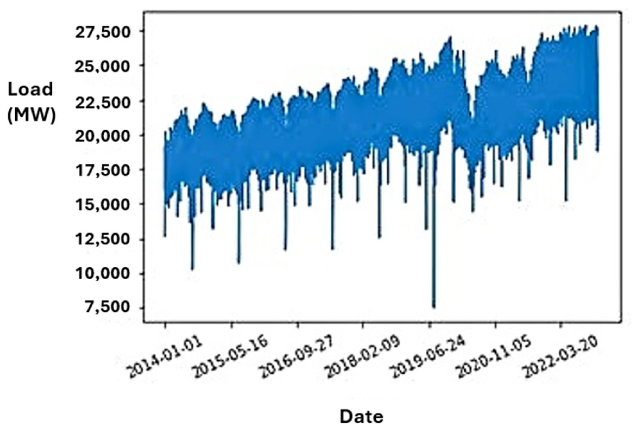
In this research, the author attempts to explain the findings obtained from an extensive data collection spanning almost a decade, which includes load data taken from the leading electric power system in Indonesia, specifically from Java Island. The comprehensive dataset, covering approximately nine years, is a testament to the meticulous data collection efforts undertaken by the researchers. Figure 1 is a visual representation that summarizes the temporal evolution and complex dynamics inherent in the collected dataset. Such comprehensive data acquisition underscores the rigor of the research methodology. The analysis was conducted using open-source Python libraries without the use of any commercial software or specialized equipment. This approach provides a strong foundation for further analysis and insights to enhance our understanding of the complexity inherent in Indonesia’s electricity system landscape.

Figure 1 illustrates a discernible ascending trajectory within the dataset, indicating a pronounced increasing trend over the observed period. Furthermore, Figure 2 offers a comprehensive cross-sectional perspective, facilitating a deeper understanding of the dataset’s multifaceted characteristics. The conspicuous perturbation observed circa 2020 is particularly noteworthy, attributed to the unprecedented policy interventions instigated in response to the global COVID-19 pandemic. This notable disruption underscores the profound impact of external socio-economic factors on the dynamics of the observed phenomenon, thereby warranting meticulous consideration in subsequent analytical interpretations and model formulations within the scholarly discourse.

Figure 2 depicts the trend in load variation over nine years, specifically observed at 13:00 h. This data segment comprises one of the 48 data points per half-hour interval within 24 h. Notably, during the onset of the COVID-19 pandemic, from 2019 to the end of 2020, discernible anomalies emerged compared to the trends observed over the preceding 5-year period. This observation underscores the necessity for adjustments in load forecasting methodologies to attain enhanced accuracy amidst evolving circumstances, thereby ensuring the reliability and efficiency of the forecasting process.

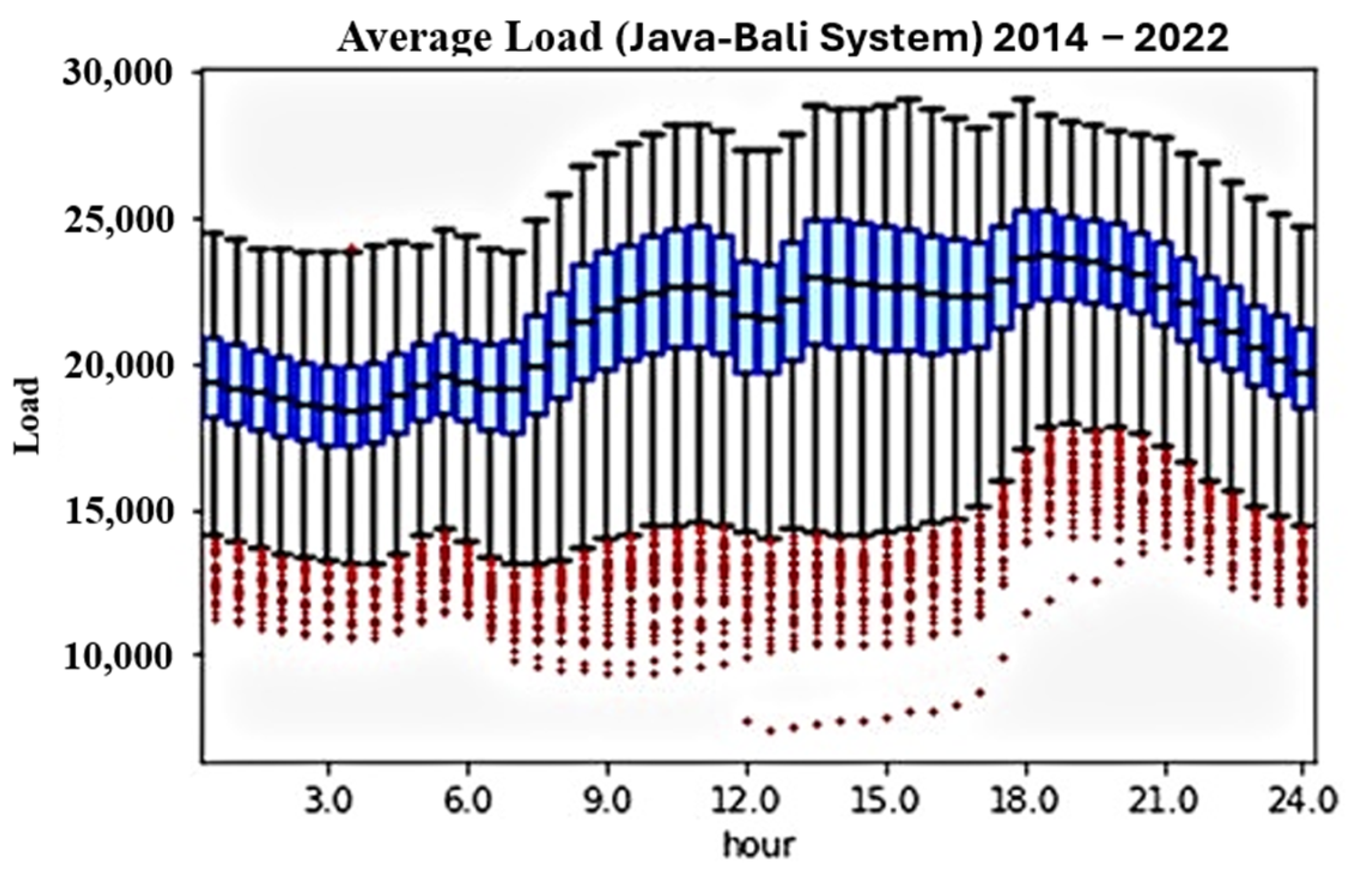
Figure 3 illustrates the average load of the Java-Bali System through a series of boxplots. The data spans from 2014 to 2022. The blue boxes represent the interquartile range (IQR), encompassing the first quartile (Q1) to the third quartile (Q3). Outliers, denoted by red-colored points below the whiskers, indicate instances of significantly divergent usage compared to other periods. This visualization encapsulates several noteworthy phenomena, prominently characterized by a pronounced decline in load, notably attributable to the significant reduction observed during the annual Eid al-Fitr holiday period. This phenomenon underscores the dynamic nature of load patterns within the region, highlighting the influence of cultural and societal factors on energy consumption behaviors. Such observations contribute to a nuanced understanding of load dynamics, which is crucial for refining forecasting models and developing strategies to effectively manage energy demand fluctuations, particularly during cultural significance periods.

By looking at the methodology in Figure 4, the authors would like to explain the 3 methods that will be used in this research as follows.

2.1. Polynomial Regression Method

This method extends a simple linear method using time series data obtained from electrical loads. Instead of utilizing only one term, this method incorporates multiple terms (n-term) to capture more complex patterns and trends in the data. The polynomial equation method is as follows:

$$Y=P_n\left(X\right)=b_0+b_{1}X+b_2{X}^2+\dots +b_n{X}^n+\mathit{\epsilon },$$

(1)

where

• Y = Forecasting result at time x;
• X = time x of the time series to be predicted;
• P_n = n-degree polynomial;
• b_i = coefficients of P_n(x) in the i-th position;
• ε = residual error.

The b_i coefficients are calculated to minimize the error using various mathematical techniques such as ordinary least squares (OLS) method or gradient descent.

The dataset at our disposal comprises half-hourly measurements spanning a full 24 h cycle, thus yielding 48 distinct time series data points per time step. The selection of a 30 min (half-hourly) sampling interval is based on the actual data availability and standard operational resolution used by power utilities in load monitoring systems. Consequently, the variable X assumes an array structure with 48 entries, encapsulating the multifaceted temporal dynamics inherent to the system under scrutiny. Nevertheless, it is imperative to underscore that the current methodological framework needs to be revised to accommodate the nuanced temporal intricacies associated with weekdays, weekends, and holidays within the dataset. This notable limitation underscores an area ripe for exploration and enhancement, as it represents an opportunity to refine our analytical approach by incorporating temporal granularity, thereby enriching the fidelity and applicability of our predictive models in real-world scenarios.

Before model training, a preprocessing step was conducted to identify and treat outlier values in the time series dataset. Outliers were detected using the Interquartile Range (IQR) method, which flags data points that lie more than 1.5 times the IQR above the third quartile or below the first quartile. Rather than eliminating these points, they were corrected using linear interpolation between adjacent valid values to ensure temporal continuity. This approach preserves the sequential structure of the data, which is essential for maintaining the integrity of time-dependent forecasting models.

2.2. Split Linear Regression Method

This approach builds upon prior methodologies by incorporating a nuanced consideration of temporal dynamics, particularly distinguishing between weekdays, weekends, and holidays within the system. Notably, weekends are operationally defined as encompassing Sundays, public holidays, and a two-week window surrounding the Eid al-Fitr holiday, irrespective of their position in the weekly calendar. This delineation prompts the development of two distinct predictive models: one tailored for forecasting load during standard working days (weekdays) and another optimized for holiday periods (weekends). By bifurcating the predictive framework, we can meticulously evaluate the efficacy and robustness of each model in capturing the nuanced load patterns inherent to differing temporal contexts. This tailored approach enhances the granularity of load forecasting and underscores the necessity for adaptive methodologies that account for temporal variations with precision and efficacy. The data-splitting procedure used to distinguish between these temporal categories is illustrated in Figure 5. Furthermore, this forecasting method stands out due to its unique approach of splitting the data into half-hour intervals, distinguishing it from other existing papers. As a result, it produces a comprehensive 24-h load curve for mid-term load forecasting.

2.3. LSTM Method

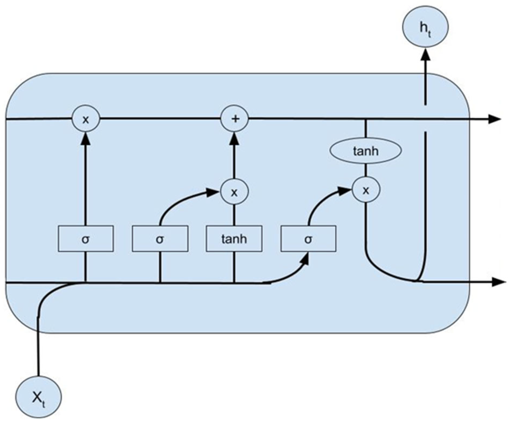
The method under consideration pertains to a specialized class of neural network architecture known as Long Short-Term Memory (LSTM), engineered specifically to discern and incorporate prolonged dependencies within sequential data streams adeptly. The foundational architecture of LSTM entails an interconnected array of memory cells strategically designed to facilitate recurrent connections. Each memory cell within this intricate framework is equipped with distinct components, including but not limited to an input gate, a forget gate, and an output gate, meticulously calibrated to modulate the flow of information circulating throughout the network. The architectural structure of the LSTM model employed in this study is illustrated in Figure 6. Given that LSTM models are susceptible to abrupt anomalies in sequential data, the preprocessing step described earlier, specifically the outlier detection using IQR and correction via linear interpolation, was especially critical. This ensured that spurious spikes or dips in the input data did not propagate through the memory gates and negatively affected the model’s ability to capture long-term dependencies. Such meticulous gating mechanisms afford the LSTM model a heightened capacity to discern and retain salient temporal patterns across extended data sequences, thereby furnishing an invaluable tool for the comprehensive analysis and prediction of dynamic sequential datasets prevalent across various academic and applied domains.

A simple five-layer LSTM with flexible window size is used in this method.

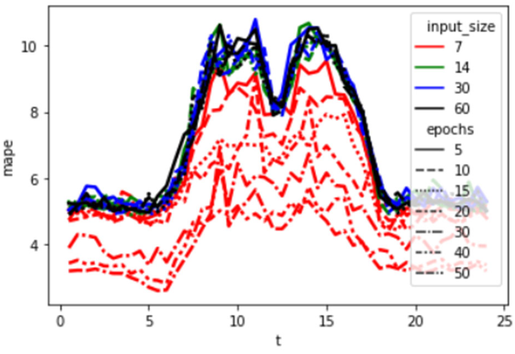
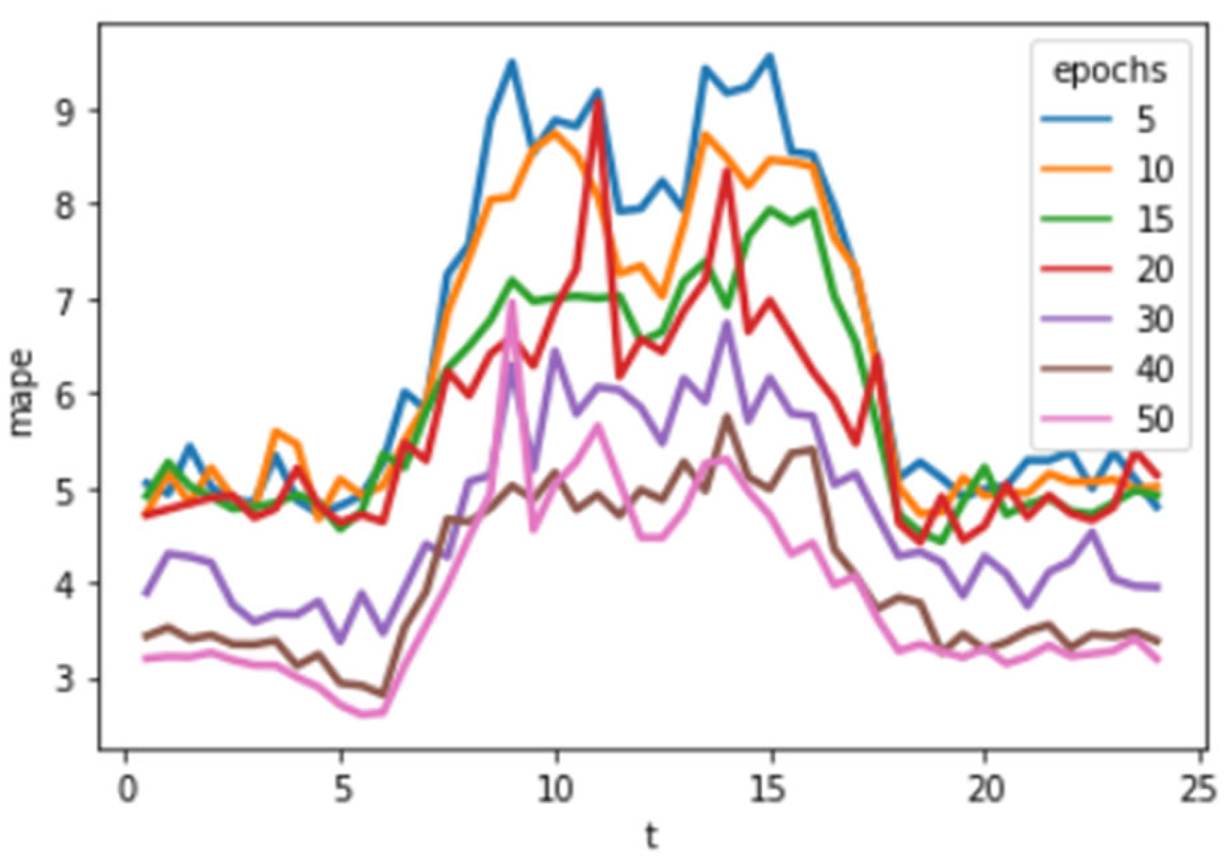
The LSTM model used in this study adopts a five-layer architecture with 64 hidden units per layer. A dropout rate of 0.2 is applied to reduce overfitting, and the Adam optimizer is used with a learning rate of 0.001. The model is trained with a batch size of 32 over 100 epochs. These hyperparameters were determined through initial trials to strike a balance between accuracy and computational efficiency.

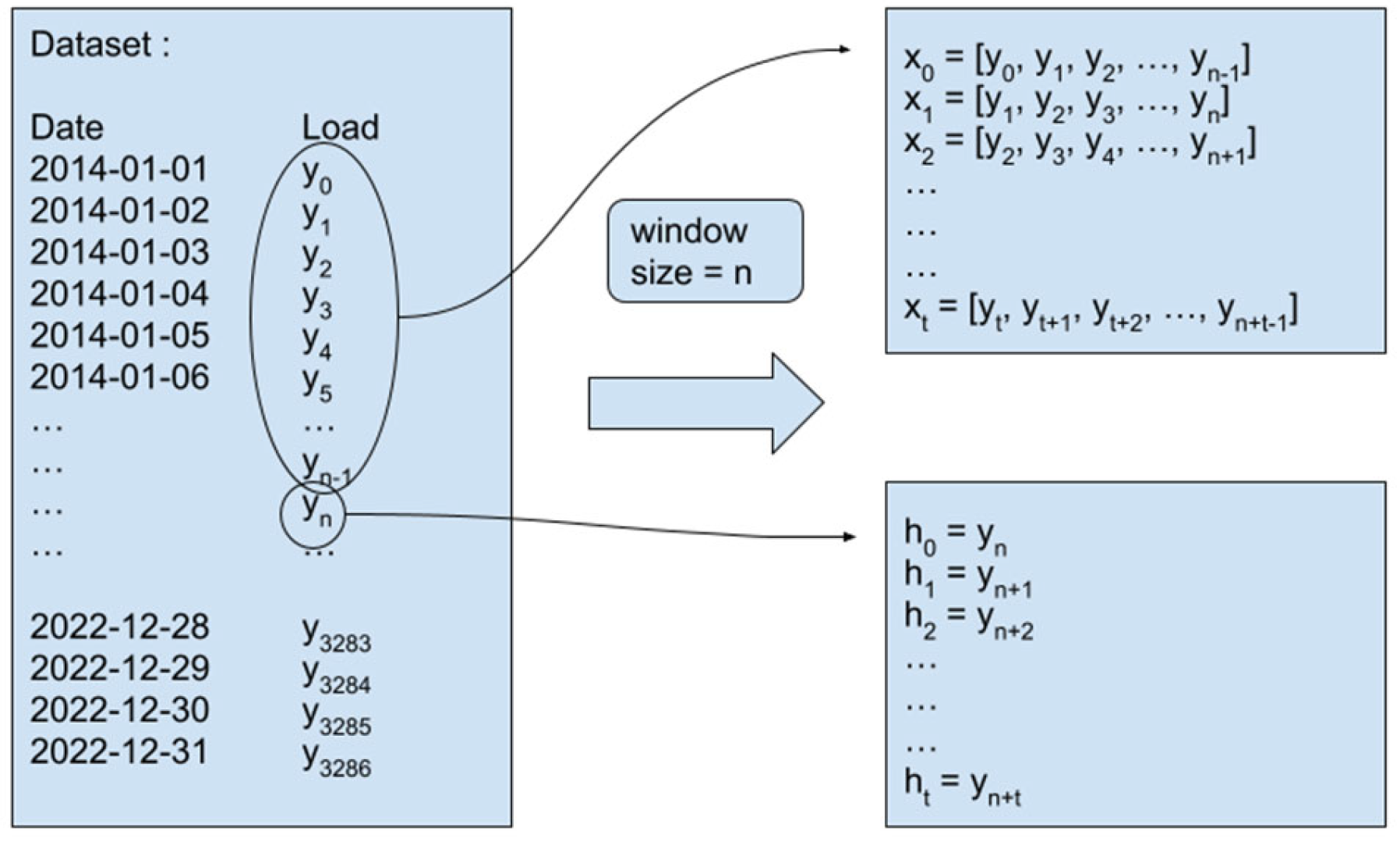
To advance predictive accuracy and robustness, the trio of methods under scrutiny undergo a rigorous training regimen utilizing data from 2014 to 2021. As shown in Figure 7, a sliding window technique is applied to generate sequences from the original time series dataset. This approach segments the data into overlapping sequences that serve as inputs for the model, enabling the network to learn temporal dependencies effectively. This meticulous training phase primes the models to capture the underlying patterns inherent within the dataset and ensures their adaptability to evolving trends and dynamics over time.

The dataset was split chronologically to simulate realistic forecasting conditions. Data from 2014 to 2021 were used to train the models, while 2022 data was exclusively used for testing and evaluation. Subsequently, armed with the insights gleaned from the training phase, these finely tuned models are deployed to forecast the load for the year 2022. The resultant predictions are meticulously juxtaposed against observed data, facilitating a comprehensive evaluation of their predictive efficacy. To quantify the comparative performance of each method, two widely acknowledged metrics, namely Mean Absolute Percentage Error (MAPE) and Root Mean Square Error (RMSE), are computed. This methodological approach not only underscores a systematic and empirical evaluation framework but also signifies a novel endeavor in leveraging historical data to inform future predictions, thereby contributing to the ongoing discourse surrounding data-driven decision-making methodologies in predictive analytics.

3. Results and Discussion

3.1. Polynomial Regression

Implementing polynomial regression in load forecasting offered a traditional yet robust approach. This method aimed to capture underlying trends and patterns in electricity demand by fitting polynomial functions into historical data.

We ran several simulations with different parameters to find the best model in polynomials. The best results are shown in Figure 8. However, our analysis revealed limitations in adapting to the dynamic nature of post-pandemic load profiles in the tropical region. While informative, the resulting Mean Absolute Percentage Error (MAPE) and Root Mean Squared Error (RMSE) metrics indicated a moderate accuracy level. While dependable for specific forecasting scenarios, polynomial regression may not be the most suitable choice for addressing the nuanced challenges posed by the post-pandemic era.

We found that the forecasting error also exhibited an upward trend as the polynomial degree increased. This counterintuitive outcome suggests that higher-degree polynomials tend to overfit the historical data, capturing noise rather than genuine load patterns. Consequently, the resulting models demonstrated reduced generalization capability, leading to higher errors in predicting future load demands. As shown in

Table 1. MAPE and RMSE Results for Polynomial Regression Models (Degree 1 to 6).

Parameter n	Name	MAPE	RMSE
1	linear	7.63	2070.67
2	quadratic	8.48	2283.32
3	cubic	8.64	2327.72
4	quartic	7.14	2148.04
5	quintic	18.88	5395.27
6	hexic	27.95	7946.36

, although the quartic model yielded the lowest MAPE value of 7.14, the errors significantly increased for higher degrees, such as quintic and hexic, reaching MAPE values of 18.88 and 27.95, respectively. This finding underscores the importance of carefully selecting the polynomial degree in load forecasting, as an overly complex model may not necessarily yield better results, especially in the context of post-pandemic load patterns in a tropical region.

3.2. Split Polynomial Regression

As an extension of the traditional polynomial approach, split polynomial regression enhances forecasting accuracy by segmenting the data into distinct periods or regimes. This method recognized that load behavior can significantly differ between various times of the day and year. Our findings improved prediction performance compared to standard polynomial regression, particularly during daytime hours. As illustrated in Figure 9, the Mean Absolute Percentage Error (MAPE) of split polynomial regression varies across different timesteps, indicating the model’s sensitivity to temporal segmentation. Furthermore, Figure 10 presents a comparison of MAPE curves for different time-based categories weekday, weekend, and holiday, and all periods showing how model performance differs significantly across temporal contexts. However, it is still necessary to work on accommodating the variability of post-pandemic load patterns, leading to suboptimal results during the weekend and holiday periods. It highlights the importance of considering more adaptive methods for load forecasting in regions experiencing significant demand fluctuations.

3.3. Long Short-Term Memory (LSTM) Network

In contrast to the traditional regression-based approaches, LSTM, a deep learning technique, has emerged as the standout performer in load forecasting for the post-pandemic tropical region. Leveraging its ability to capture intricate temporal dependencies, LSTM exhibited remarkable accuracy with a MAPE of 3.86% and an RMSE of 1247.93 with seven days of data input. Furthermore, it demonstrated consistent excellence in load prediction, irrespective of the time of day.

As illustrated in Figure 11, a meticulous examination reveals that employing a 7-day input window is the optimal strategy for generating precise forecasts regarding the subsequent day’s load demands. This nuanced observation underscores the significance of temporal contextualization and historical data aggregation in enhancing predictive accuracy within the domain under investigation. Moreover, the elucidation provided in Figure 12 furnishes a deeper analytical dive into the intricacies encapsulated within this discerning diagram, shedding light on the underlying mechanisms and causal relationships that govern the observed phenomena. This empirical exploration contributes to the expanding body of knowledge in predictive modeling methodologies by unraveling such complexities. It underscores the critical role of informed parameter selection in optimizing predictive performance, thereby advancing the frontiers of academic inquiry in data-driven decision-making processes.

To contextualize this study’s findings,

Table 2. Positioning This Study Within Recent Load Forecasting Research.

No.	Author(s) and Year	Method(s) Used	Horizon	Region/System	Accuracy (MAPE/RMSE)
1	Baek [1]	Recurrent Neural Network	Mid-term	Korea	MAPE ≈ 4.12%
2	Jiang et al. [2]	Probabilistic models + Spark	Mid-term	China	RMSE not specified
3	Xu et al. [3]	Hybrid Deep Learning (CNN-LSTM)	Short and Mid-term	China	MAPE ≈ 5.02%
4	Bouktif et al. [8]	LSTM-RNN + Metaheuristics	Short-term	UAE	MAPE ≈ 2.60%
5	Sun et al. [10]	Time-Series Decomposition + ELM	Short-term	China	RMSE ≈ 1360
6	Jember et al. [11]	LSTM + Forecast-based energy share	Mid-term	Smart grid community	MAPE not specified
7	This Study	Polynomial, Split Poly., LSTM	Mid-term	Indonesia (Java-Bali)	MAPE = 3.86%; RMSE = 1247.93

presents a comparative summary of recent works in load forecasting, highlighting their methodologies, forecasting horizons, application regions, and accuracy levels. This comparison further emphasizes the proposed LSTM-based approach’s performance and relevance in addressing medium-term forecasting challenges in tropical, post-pandemic settings.

Furthermore, accurate forecasting models such as LSTM have potential economic implications, including reduced generation costs, optimized fuel planning, and improved grid operations reliability. While this study focuses on methodological evaluation, future research should include real-world deployment scenarios to assess operational impacts and cost savings in practical settings.

4. Conclusions

In conclusion, this study presents a comprehensive analysis of medium-term load forecasting in post-pandemic tropical regions, focusing on the comparative evaluation of three different methods: polynomial regression, discrete polynomial regression, and Long Short-Term Memory (LSTM) networks. The goal is to improve our understanding of load prediction accuracy in this evolving context.

Our investigation revealed clear and interesting results: LSTM, a deep learning technique, outperformed other methods, showing unmatched accuracy with a Mean Absolute Percentage Error (MAPE) of only 3.86% and a Root Mean Squared Error (RMSE) of 1247.93. These observations underscore the potential of deep learning in capturing complex electricity demand dynamics, even in the face of post-pandemic uncertainty.

Additionally, a consistent trend emerges from our analysis, showing that all methods consistently outperform in load estimation during the night, from 6:00 p.m. to 6:00 a.m. We hypothesize that the inherent stability of the data during these hours, characterized by reduced fluctuations, contributes significantly to the observed improvement in prediction accuracy.

This study also acknowledges that the influence of outlier handling methods on model performance, particularly for deep learning-based forecasting, warrants further exploration. Future research may include comparative analyses between raw and cleaned datasets to quantify this effect and evaluate model sensitivity to anomalous data.

However, a notable and significant new finding that deserves highlighting is the success of LSTM in addressing the unique challenges posed by COVID-19, which resulted in substantial anomalies in overall electricity demand patterns across large-scale systems. With its high accuracy, LSTM proves adept at capturing and anticipating these changes effectively, showcasing remarkable potential in confronting uncertain and dynamic conditions. The implications of this finding are highly relevant in the context of post-pandemic electricity network management, where resilience to demand fluctuations becomes increasingly critical in large-scale load forecasting.

From an operational standpoint, the LSTM-based approach is particularly promising for improving scheduling decisions, reducing reserve margins, and supporting more efficient resource allocation within power systems. Future studies may further explore ensemble forecasting models or real-time adaptive retraining mechanisms to enhance model robustness and adaptability in evolving load environments. Thus, while our analysis underscores the superiority of LSTM in load forecasting, this technique also holds promise as an adaptive and reliable solution to tackle future challenges in an ever-changing environment.