Abstract
Maintenance techniques are fundamental in the context of the safe operation of continuous process installations, especially in electrical energy-transmission and/or -distribution substations. The operating conditions of power transformers are fundamental for the safe functioning of the electrical power system. Predictive maintenance consists of periodically monitoring the asset in use, in order to anticipate critical situations. This article proposes a methodology based on data science, machine learning and the Internet of Things (IoT), to track operational conditions over time and evaluate transformer aging. This characteristic is achieved with the development of a synchronization method for different databases and the construction of a model for estimating ambient temperatures using k-Nearest Neighbors. In this way, a history assessment is carried out with more consistency, given the environmental conditions faced by the equipment. The work evaluated data from three power transformers in different geographic locations, demonstrating the initial applicability of the method in identifying equipment aging. Transformer TR1 showed aging of , followed by TR2 with and TR3 showing in the evaluated period of time.
1. Introduction
The high acquisition cost of a power transformer and the inherent difficulty in its maintenance, due to its large physical dimensions, make it necessary to develop techniques that increase assertiveness in maintenance tasks. Another critical aspect involves the different parties engaged in the operation of power transformers, both directly and indirectly [1,2,3,4,5,6,7,8,9].
The parties involved in the process include maintenance and operation teams, which represent the distinct perspectives of the companies owning the transformer. In the case of the operations team, there is a desire for full availability of the asset for its intended use in company activities. The maintenance team, on the other hand, is responsible for keeping this asset available for use.
Other important viewpoints are those of the asset manufacturer and regulatory agencies. For the manufacturer, it is essential that the asset meets the conditions of the sales contract, especially the contracted factory warranty period. Regulatory agencies are responsible for overseeing the operation of the item.
Finally, customers are the main stakeholders in service continuity, as they require the full operation of the asset for their daily activities. The main objective of the power transformer is to meet the expectations of the customers connected to its output bus.
To illustrate the importance of power transformers and the need to develop new techniques, we can mention a significant power transformer failure that severely affected the state of Amapá, in northern Brazil. On 3 November 2020, a transformer at the main substation in Macapá failed, causing a statewide blackout [10,11,12].
The main conclusions indicate that the disturbance originated from a short circuit in the transformer, due to a possible internal equipment failure [10]. The damaged transformer had 230/69/13.8 kV–150 MVA characteristics and was responsible for 50% of the load in Amapá. A load-rotation system was set up, together with the activation of diesel-fueled thermal generating units, totaling 24.28 MW of installed power, to mitigate the problem [13,14,15,16].
Only on 24 November 2020, with a replacement transformer, was normal electricity supply restored in the region [13,14,15]. The Brazilian Electricity Regulatory Agency (ANEEL) fined the utility company BRL 3.6 million as a result of the power interruption [17].
This incident highlights the need for research in the area of predictive maintenance applied to power transformers, especially considering that in Brazil, from 2021 to 2025, there is an estimated average load growth of 3.6% per year. The average load is projected to reach 79,600 MW by 2025 [18].
The proposal aims to construct a methodology based on Machine Learning (ML) and the Internet of Things (IoT) to develop a predictive maintenance system for power transformers in electrical substations. This system is of significant value given the importance of transformers for the safe operation of the power system.
Previous studies have explored aspects related to the work proposed here, but further developments are still possible. The recent advancement of microcontroller technology enables the creation of embedded devices with substantial digital data-processing capabilities, ushering in an era of advanced possibilities [19].
In this context, devices are interconnected in networks, enabling high-speed and reliable data exchanges, as well as access to resources and services on other physically separated devices—sometimes by hundreds of kilometers [20,21,22].
Based on this context, new technologies and concepts for device integration have emerged, known as the Internet of Things (IoT) [21,22]. This opens up a vast range of applications for the power system. One can envision interconnected devices with high processing capacity, performing real-time power flow calculations, rapidly reconfiguring the network during critical events [23].
Machine Learning (ML) refers to a set of techniques that enable computer systems, based on adequate data histories, to make future predictions regarding variable behaviors. Among the main ML methods are fuzzy logic and Artificial Neural Networks (ANNs) [24,25,26,27,28].
ANNs have been used in works related to load forecasting [29] and the identification of non-technical losses in irrigated farms [30]. In the context of transformers, ref. [31] developed an ANN-based system to estimate the amount of furan in transformer oil. In [32], a case study that classifies failures in transformers using ANNs is presented. ANNs are also used in the analysis of dissolved gases [33] and in estimating transformer hot spots [34].
Ref. [35] used fuzzy logic in the context of prioritizing maintenance for SF6 gas circuit breakers in substations, developing a fuzzy system for this purpose. Ref. [36] developed an operational vulnerability indicator for prioritizing transformer replacement, complementing the conventional Health Index methodology. Ref. [5] evaluated the structural importance of transformers based on the composite H2 reliability index, developing a new methodology for calculating the Health Index. These contributions can be further extended with IoT technologies and different machine learning applications.
The Health Index constitutes a widely used methodology in the electrical sector, especially among electric utilities, for verifying the reliability level or health condition of an asset [2,37]. The indicator is based on the weighting of multiple individual factors regarding the transformer or equipment under analysis and is the main tool to assist in maintenance decision-making [38,39,40,41,42,43,44,45].
Based on the above, it is evident that further research opportunities exist, especially with respect to system integration. More assertive predictive maintenance models can be developed by incorporating new technologies and analysis tools [46,47,48,49,50,51,52]. Environmental and economic benefits are expected from these proposals, as optimizing predictive maintenance processes eliminates unnecessary activities, reduces waste of inputs such as transformer oil, and minimizes the cost of dispatching teams [6,7,8]. The operating conditions of equipment and its installation environment can compromise its long-term reliability [53,54].
In the current context of energy transition, integration with different energy sources becomes fundamental for the safe and reliable operation of the power system [55]. Power transformers are one of the main links of integration, as they enable interconnection between different voltage and power levels to meet the local needs of load and generation. The transformer becomes an essential element for long-distance energy transmission.
The interior of a power transformer—its active part, called the core—consists of copper windings wrapped in insulating paper. The copper winding is wound on a ferromagnetic material, usually silicon steel, to better conduct magnetic flux. The core is immersed in mineral oil to facilitate heat transfer to the external environment. Such materials can be easily consumed in a fire caused by an internal failure.
A failure in one of these devices has major consequences for the quality of electricity supplied to consumers, causing disruption to daily life and production losses for local businesses. These inconveniences are coupled with serious environmental issues, as failures often lead to severe fires, which result in pollution from toxic smoke and the use of large amounts of water to contain the flames.
The article is based on a methodological demonstration for creating operating profiles for transformers under evaluation, contributing to the planning of preventive maintenance activities. Currently, the Health Index consists of a common methodology in electric power systems. However, the Health Index will only produce reliable results if fed with reliable data. In this sense, not considering tangible thermal stress data may create unrealistic results.
This article contributes to this aspect by estimating thermal profiles in the geographic coordinates of substations. This fact allows the use in remote locations or small-scale installations, without advanced monitoring resources, or even in various industrial installations. A historical thermal profile can be developed for the geographic location of interest.
The next sections present a review of related works and the method, demonstrating the applicability of the proposal. This is followed by the presentation and discussion of results and methods. The work concludes with final remarks and points to potential future developments.
2. Related Works
Vianna [35] describes a new methodology for prioritizing the maintenance of SF6 Gas Circuit Breakers, based on the development of a Composite Risk Index (CRI), which consists of two main components: Basic Condition (BC) and Operational Condition (OC). The BC component arises from a system utilizing Fuzzy Logic, combining information about life cycle, wear and aging, and maintenance history. Such data are processed using specific fuzzy membership rules. In the final step, the BC index is combined with the OC indicator through another Fuzzy system to extract the CRI, which classifies the circuit breaker. The OC indicator signals the existence of anomalies or defects in the equipment that may impair substation operation. In his work, ten circuit breakers from a substation in the state of Rondônia were evaluated.
When it comes to estimating the concentration of dissolved gases in power transformers, Pereira [56] implemented an application of Nonlinear Autoregressive Neural Networks (NAR), combined with discrete Wavelet Transform. The gases considered include hydrogen (H2), carbon monoxide (CO), methane (CH4), carbon dioxide (CO2), ethane (C2H6), ethylene (C2H4), and acetylene (C2H2). Real transformer data were used, and the solution was compared to time series analysis techniques such as Autoregressive Moving Average Model (ARMA), Autoregressive Integrated Moving Average Models (ARIMA), and Seasonal ARIMA (SARIMA). The neural network was trained using 80% of the samples for training and 20% for validation. It was found that the model was able to predict gas concentrations with a maximum error of 6.03% for hydrogen and 0.34% for carbon dioxide.
As for prioritizing the replacement of power transformers, Schmitz et al. presented in [36] an Operational Vulnerability Index (OVI) as an improvement to the conventional Health Index methodology. Inspired by the work of Vianna [35], the OVI specifically addresses power transformers. The index considers Technical Condition (TC) and Operational Condition (OC). Distinctively, the TC component accounts for operational parallelism and the presence of spare transformers. The transformation ratio is also considered, since the higher its value, the more complex the transformer’s construction—requiring more insulating material. For the OC component, results from dissolved gas tests and insulating oil analysis are mainly employed. The Preference Ranking Organization Method for Enrichment Evaluations (PHROMETHEE) ranks the most critical transformers, and the Analytic Hierarchy Process (AHP) defines criterion weights. A sample of 39 transformers from seven substations were classified.
Regarding Health Index methodologies, Velasquez [37] developed a novel model applying Wavelet Networks. Test results from oil analysis—including dielectric strength, moisture content, and power factor—are combined with dissolved gas analysis. Numerical values are assigned to different measurement ranges, constructing an index. This solution was compared against a decision tree in classifying 48 transformers and reactors, all rated at 500 kV.
A methodology for deciding maintenance strategies in power transformers was implemented by Dong et al. [57]. Transformer operational condition is based on the analysis of dissolved gas tests, physico-chemical oil tests, and electrical tests. Historical maintenance data are also evaluated to suggest future actions. An economic analysis is presented, considering revenue loss due to potential transformer failure. The model is optimized through Particle Swarm Optimization (PSO). However, the authors did not report algorithm execution times or cost reductions in the maintenance process.
Feil [5] proposed a multi-criteria methodology for power transformer replacement decisions. The approach takes into account transformer lifetime and failure risk factor, as well as the systematic importance through equipment impact on the electrical system. The technical aspects guiding transformer replacement decisions include the Health Index (HI), Equivalent Aging Factor (FEQA), and composite reliability indices such as Loss of Load Duration (LOLD), Loss of Load Frequency (LOLF), Expected Energy Not Supplied (EENS), and the Severity Index (SI), which weights the equivalent duration in minutes of peak load loss. The Analytic Hierarchy Process (AHP) is employed to rank which transformers should be replaced.
In [58], a new transformer failure rate model considers the impact of maintenance based on data mining of daily chromatographic oil monitoring. To ensure modeling data quality, an enhanced k-Nearest Neighbors (k-NN) algorithm based on Genetic Algorithms (GA) is proposed to repair missing monitoring data. A Multi-Back-Propagation Neural Network is then implemented to estimate the time to failure based on the processed data, and the method is compared with a four-state Markov chain. Nevertheless, details about data acquisition or execution of the proposed method are not emphasized.
Foros et al. (2020) [59] presented a method that estimates transformer health based on coil degradation modeling, Health Index, and historical operation statistics. These indicators are combined to create the Apparent Aging indicator, from which a risk indicator is determined. This risk indicator supports the assessment of transformer failure severity in its system and aids in maintenance and replacement planning.
In his work, Fauzi [60] describes a data mining framework applied to optical spectroscopy measurement of transformer oil. The correlation between optical features from 2120 nm to 2220 nm and dissolved gas analysis, including Duval Triangle interpretation, shows that low-energy electrical discharges, high-energy electrical discharges, and thermal faults at temperatures above 700 °C can be accurately predicted in power transformers. The authors report an accuracy of 98.1%.
Dias et al. [61] implemented an Internet of Things (IoT)-based system for real-time monitoring of high-voltage transmission lines, focusing on delta towers. The solution involved instrumenting the support cables with tension sensors to measure structural forces due to wind. In addition, wind speed and direction sensors, as well as accelerometers for vibration measurement, were installed. A wireless IEEE 802.15.4g/e network was used for data acquisition, and a central framework processed historical data.
A system for monitoring the operational condition of power transformers using a wireless sensor network is detailed by Chen [62]. The paper concentrates on the technique for predicting transformer anomalies. The proposed solution combines a Grey Prediction Model (GPM) with genetic algorithms and particle swarm optimization, resulting in a hybrid algorithm. GPM is used to estimate gas concentrations over short periods; its estimation parameters, and , are optimized by combining algorithms. This hybrid approach is said to detect anomalies faster than other methods, although performance evaluation is not discussed in detail.
Freitag and colleagues [63] designed a framework to evaluate power system reliability under severe weather conditions. Meteorological data were obtained from the National Institute of Meteorology (INMET), and Monte Carlo simulations were applied to qualify the impact of weather conditions on the reliability of the power grid.
Turning to temperature estimation in transformers, Kaminski [34] proposed a methodology for estimating top-oil temperature and consequential transformer life reduction. The work utilizes Non-linear AutoRegressive with eXogenous inputs (NARX) neural networks. Results show an error of approximately 2 °C when estimating temperature compared to historical data. The network uses ambient shaded temperature, transformer power output, and the number of active fans as inputs. Data from three hydroelectric generator transformers rated at 330 MVA, with voltages from 13.8 kV to 525 kV, were used.
A system based on Mobile Edge Computing (MEC), implemented on a Raspberry Pi 3, was developed by Franco [64]. This embedded device provides functionalities for predictive maintenance, including internal storage and data-processing routines to create machine learning models. While hardware limitations restrict large-scale data insertion and result in longer processing times compared to desktop workstations, the flexibility of the solution compensates for these drawbacks.
Regarding asset management support, Campanhola et al. [9] implemented a management tool for the power system focused on power transformers. The tool considers equipment lifetime, system criticality, financial aspects, and electricity demand forecasts to assist utilities in medium- and long-term planning. The Analytic Hierarchy Process (AHP) multi-criteria method weights the criteria based on expert opinions, classifying the most critical equipment in the study system. Monte Carlo simulation is combined to model future loading scenarios, evaluating a transformer’s future criticality. The methodology is applied to a real transformer fleet over a 10-year horizon considering three distinct scenarios, thus identifying critical units.
3. Materials and Methods
Based on the historical data of the transformer and the climatic conditions to which it is subjected, a model for estimating its aging can be developed. The processing of large datasets, through the application of data mining and machine learning techniques, along with the use of IoT technologies for real-time data acquisition, is key. The significant importance of the power transformer for the reliable and safe operation of the electrical system justifies the development of new methodologies and systems aimed at predicting its operational condition.
The data-acquisition stage consists of gathering a set of measurements and related information to determine both the operational conditions and, subsequently, the equipment’s degree of deterioration based on its usage. This stage is fundamental for ensuring the consistency of the aging model to be developed. The main datasets are listed below:
- Maintenance Data Acquisition;
- Weather Data Acquisition;
- Operational Data Acquisition.
3.1. Data Analysis Methodology
Data analysis is performed specifically based on the set of vectors stored in servers, traditionally in a distributed environment. Different types of data are stored with specific sampling rates according to their demands. The analysis must account for the necessity of data synchronization to avoid misleading conclusions. The developed methodology is shown in Figure 1.
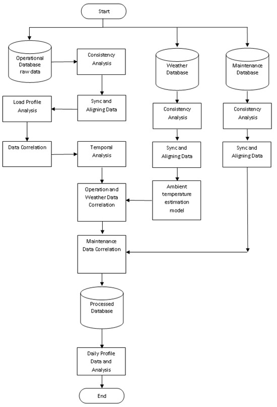
Figure 1.
Flowchart of the implemented methodology.
Using the operational data stored on servers, consistency analysis is first performed to prevent handling of empty values or repeated sequences. After consistency analysis, a synchronization and alignment of data vectors is necessary to guarantee synchronous samples. At this partial stage, correlations between electrical quantities and partial load profiles can already be extracted.
The pre-processed vectors are then correlated with climatic data, obtained from a specific database. Consistency and synchronization analysis is also performed on these. The correlation of climatic data, together with load profile extraction, allows the evaluation of external influences on transformer operational conditions.
The implementation is based on importing transformer operational data according to the previous methodology. Traditional data-acquisition systems only sample reading data, and as per the literature review, their analysis is rarely automated or performed periodically.
In this implementation, Python 3.11 is used—a general-purpose programming language that has gained prominence in recent years [65]. Pandas 2.1 is an open source library for data structuring and analysis [66]. Matplotlib 3.7.2 is a library for creating high-quality visualizations [67].
Within the proposed solution, a Python 3.11 script imports data using the Pandas 2.1 library. The read_excel method imports the data and creates a tabular structure, which can be easily manipulated using Python. Mathematical operations are performed using the Numpy 2.0 library, and Matplotlib 3.7.2 is employed to generate data visualizations for the user.
During the data analysis and transformer modeling phase, maintenance history and operational records from utility company systems are analyzed. Data mining techniques are applied to synchronize, filter, and align the different data types and sampling frequencies.
Considering common practice used in power systems, hourly samples of electrical measurements were used to compare with measurements and estimates of ambient temperature. Thus, synchronization with ambient temperatures occurs every hour. The different datasets are joined by dates.
3.2. Maintenance Database
As shown in Figure 1, the historical maintenance database are crucial for providing an overview of the transformer’s health, taking into account data available in the company’s current management systems. These data will be correlated with the climatic and operational conditions of the transformer under analysis, where failure points linked to these events will be investigated. Based on the literature review, the following data have been selected for use in the system:
- Visual inspection;
- Electrical tests;
- Oil analysis:
- −
- Visual inspection and color;
- −
- Density;
- −
- Dielectric strength;
- −
- Neutralization number;
- −
- Interfacial tension;
- −
- Moisture.
- Dissolved gases:
- −
- Hydrogen (H2);
- −
- Methane (CH4);
- −
- Ethane (C2H6);
- −
- Ethylene (C2H4);
- −
- Acetylene (C2H2);
- −
- Carbon Monoxide (CO);
- −
- Carbon Dioxide (CO2).
3.3. Operational Data
As shown in Figure 1, the operation database of a power transformer is understood as a continuous process that maintains electricity supply to consumers connected to its output bus. Changes in the consumed load generate stress conditions on the equipment and thus reduce its useful life. Based on the literature review, the following electrical and temperature measurements are considered:
- Electrical power;
- Primary voltage;
- Secondary voltage;
- Primary current;
- Secondary current;
- Top oil temperature;
- Winding temperature.
By utilizing IoT, these measurements can be acquired and shared in a cloud information system for real-time processing of operational variables. This feature allows the construction of operation and maintenance management systems integrated on a common platform.
3.4. Weather Data
As shown in Figure 1, the use of weather data allows the development of correlations with the operational conditions of the analyzed power transformer. In this context, IoT technologies will be further explored, initially by automating the capture of meteorological data from automatic weather stations of the National Institute of Meteorology (INMET). Scripts are thus used for periodic data capture. Based on the state of the art, ambient temperature or dry bulb temperature—as indicated by automatic weather stations—is the most relevant variable for automatic acquisition. Considering computational limitations with large-variable models, the main variable selected was ambient temperature.
For better comprehension, Table 1 presents the geographical coordinates—latitude and longitude in degrees—and altitude in meters, of the automatic weather stations in Rio Grande do Sul used in this article. From the transformer’s geographic location, it is possible to use climate data from the nearest stations to construct a profile of local weather conditions to which the equipment is subjected.

Table 1.
Automatic weather stations in Rio Grande do Sul.
The distribution of these stations across the region resembles a matrix configuration, allowing the use of information from nearby stations to estimate the ambient temperature experienced by the transformer. This solution is not commonly explored in related works, which often use far-away stations or only average temperatures, which does not represent the actual stress the equipment experienced in the period. Accessing the historical data offers a more accurate estimate.
Naturally, data availability is limited by the operational start date of each station. The oldest automatic stations started operating around the year 2000. In recent years, the number of available stations has increased. For earlier dates, manual stations must be used, which may exceptionally reduce the amount of data but does not make their use unfeasible.
For clarification and illustration, Figure 2 indicates the geographic locations of the automatic weather stations and the electric substations considered in this article. The application of the methodology is generic enough to include transformers at other locations, including those used in electricity-distribution networks. Industrial complex substations without constant monitoring can also be covered, requiring only their geographic location.
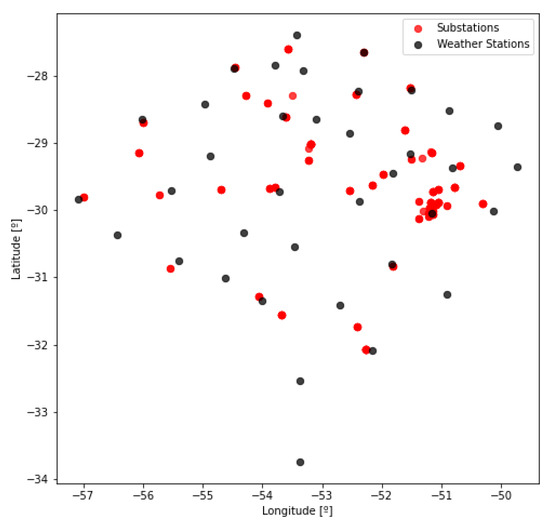
Figure 2.
Location of weather stations and electrical substations.
The distribution of meteorological stations in this territory was carried out by the National Institute of Meteorology of Brazil. The idea was to take advantage of this infrastructure to allow estimation of ambient temperatures in different locations of these stations, precisely at the locations of the transformers. With this, it is possible to estimate local temperatures based on known measurements.
Ambient Temperature-Estimation Model
As shown in Figure 1, the ambient temperature-forecasting model proposed in this article is described in this section. The initial model was based on Multiple Linear Regression. This hypothesis was tested first, developing the mathematical model shown in Equation (1). Using the geographic location and altitude of the automatic stations, the model estimates the ambient temperature at other geographic locations.
In Equation (1), coefficients X1 through X6 correspond to the linear model’s parameters. The latitude under evaluation in degrees is represented by lat, longitude by lon, altitude in meters by alt, day of the month by day, month of the year by month, and hour of the day by hour.
The input variables were selected to make the model generic. The goal is to estimate temperatures for a specific region; thus, the use of geographic coordinates is justified. In this article, the analysis is limited to the territory of Rio Grande do Sul. Given that substations are ground level, estimating temperatures at high altitudes or above ground level is out of the model’s scope. As mentioned, this initial model was based on Multiple Linear Regression. However, this technique yielded unsatisfactory results because the system exhibits non-linear behavior. In Table A1 and Table A2 model parameters are presented for better understanding.
A new approach, using the same variables, was developed with the k-Nearest Neighbors (k-NN) algorithm, in which tests for different k values were performed. With low k values, the estimated signal contained high noise levels; as k increases, the signal better fits the measured data. The final model uses and considers distance as the metric. The temperature-estimation model proposed in this article is a rarely explored contribution for aging assessment. Throughout the process, the KNeighborsRegressor class in the sklearn library was used. Figure 3 presents a general representation.
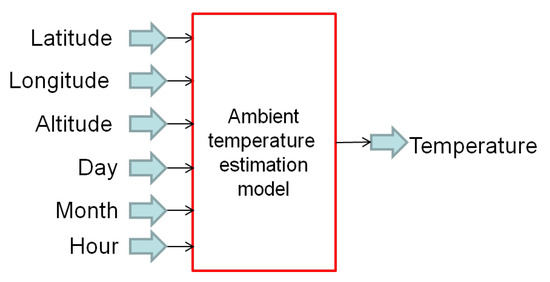
Figure 3.
Ambient temperature-forecasting model.
As input variables, information about the month of the year, day of the month, and hour of the day were added. These were simplifying assumptions to reduce model complexity. For temporal extension, the current or previous year can be added as input in the future. With historical records available, the model will estimate temperature measurements. This configuration makes the model very generic, viable even for applications in fields such as agriculture, livestock, or other industrial needs.
For the territory of Rio Grande do Sul, the latitude and longitude have negative values and use decimal degree notation. The altitude variable is defined in meters. The month variable assumes values from 1 to 12, while the day ranges from 1 to 31 as not all months have the same number of days. The hour variable ranges from 0 to 23, indicating the hours of a day. Naturally, infrequent dates, such as 29 February, will have few samples and thus rougher estimates; in this case, estimates from previous days may be reused as a similarity-based assumption.
3.5. Model Integration
The ambient temperature-estimation model is integrated with the transformer model and aging estimated using the thermal model provided by IEEE Standard C57.91-2011 [68]. This integration is outlined in Figure 4.
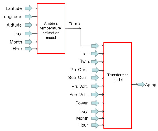
Figure 4.
Integration among models.
3.6. Aging Verification
According to IEEE Standard C57.91-2011, by using Equation (2), it is possible to compute the Aging Acceleration Factor (FAA) of the transformer. In this equation, refers to the Hot Spot temperature, indicating the highest internal temperature of the equipment. The considers a maximum temperature of 110 °C; that is, up to this value, the factor is less than unity.
Furthermore, the Equivalent Aging Factor (FEQA) for an operation period can be evaluated by Equation (3).
The percentage loss of insulation life, or %Loss of Life (), is assessed using Equation (4) from IEEE Std C57.91-2011. While a 24 h period is commonly analyzed, aggregation over longer intervals can also be performed. The standard suggests 180,000 h or 20.54 years as the useful life duration.
3.7. Data Preparation
In this article, data are normalized according to Equation (5). In this way, values are converted to a range [−1, 1] according to the properties of each variable—a widely used procedure in machine learning operations.
where, as per Equation (5), is the normalized variable value, is the original variable value, and is the absolute value of the attribute’s largest value. As such, values are [0, 1] normalized for positive attributes, [−1, 1] for positive and negative attributes, and [−1, 0] for attributes that are only negative.
3.8. Final Considerations of the Section
In the context of predictive maintenance, analyzing an asset’s operational conditions provides valuable information for making the best intervention decisions. Maintenance teams need the most accurate information possible to manage their assets. Incorrect analysis of data may lead to unnecessary or ineffective actions, potentially resulting in flawed repairs that accelerate failure mechanisms.
The proposed methodology, grounded in real-time data acquisition and processing, enables those involved in the operation and maintenance of power transformers to detect adverse operational conditions that may compromise their safe and reliable functioning.
Assessing the aging level of a power transformer contributes to increased operational safety in substations and supports operational planning, as equipment wear can be better determined or even compensated for through power network reconfiguration, redistributing load to transformers with lower loading levels at a given moment.
Considering the literature review, the ambient temperature was the most used variable, since it affects the heat dissipation to the environment. Wind, given the terrain relief conditions, is more difficult to predict, and can make the model quite complex. Rain was not considered because not all stations have hourly measurements of this variable. Thus, the model was simplified to use only ambient temperature, the most common variable, and thus reduce the computational cost.
4. Results
In this section, the results of applying the proposed methodology are presented. A case study with a set of real transformers is discussed. Initially, the validation of the climatic model is verified through the extraction of ambient temperature data. Subsequently, the analyzed transformers are indicated.
4.1. Validation of the Ambient Temperature-Estimation Model
The ambient temperature-estimation model was developed considering a set of variables for its use, as shown in Section 3. In this sense, a correlation analysis is conducted to verify the independence among the proposed variables. Table 2 presents the Pearson correlation coefficient for each variable.
Table 2.
Pearson Linear Correlation.
As shown in Table 2, the low values indicate the absence of correlations. The only relevant case, albeit of low intensity, is the relationship between the measured ambient temperature and the month of the year, which is naturally in line with expectations.
Figure 5 presents a graphical representation of the verification process for the k-Nearest Neighbors model, used for local ambient temperature estimation. A script performed the task of training and verifying the model, using the technique of splitting the data into two parts: one for training and the other for verification. In this article, 70% of the data is reserved for training and 30% for verification, a technique that is quite common in related works.

Figure 5.
k-Nearest Neighbors model verification.
The values in each data split are shuffled and presented to the model. The number of k-neighbors is chosen to be odd to avoid ties in neighbor selection, and the exact number of neighbors is determined through model performance tests. Values of 3, 5, 7, and 9 were tested for k, as shown in Figure 5. For low values of k, the model exhibited a high incidence of noise, while for high values of k, the model produced estimates with little adherence to the data, attenuating the signal amplitude. Table 3 presents the final parameters of the model using , which provided the best results. In this article the distance vector was the metric for the clusters, as common practice in related works.
Table 3.
k-Nearest Neighbors final model parameteres.
A verification of the ambient temperature estimation generated by the final k-Nearest Neighbors model, using the geographical coordinates of a transformer (TR1) located in the city of Gravataí, is shown in Figure 6.
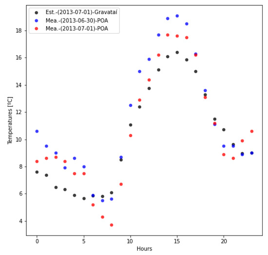
Figure 6.
k-Nearest Neighbors model temperature estimation for Gravataí city.
In Figure 6, the estimation is compared with real data from the nearest automatic weather station, in this case, located in the city of Porto Alegre. The day 1 July 2013 was arbitrarily selected for the test. The signal is also compared with that of the previous day from the same station. The model with was the one that most accurately captured the behavior of the measurement patterns. For other values, the generated signals exhibited either excessive noise or significant attenuation.
4.2. Evaluated Transformers
In this implementation, data vectors containing measurements of electrical power, primary and secondary voltages of the transformer, currents, oil temperature, and current TAP position were acquired at 15 min intervals. A total of 17,639 records were collected between “T00:00:00” on 1 July 2013 and “T23:45:00” on 31 December 2013. The climatic data analyzed in the previous section also correspond to this same period.
The acquired dataset makes it possible to visualize the behavior of the operating variables of transformers under normal operation. In this work, data vectors were obtained from three-phase power transformers. For simplicity, the nomenclature used is TR1 for a transformer located in the city of Gravataí, TR2 for a transformer in the city of Caxias do Sul, and TR3 for a transformer in the city of Venâncio Aires. All these cities are located in the state of Rio Grande do Sul, Brazil. For clarification, in this work, the choice of transformers, was based on the availability of data. Authors did not have access to more transformers.
Table 4 shows the characteristics of the analyzed transformers. In this article, the geographic location corresponds to the substation where the equipment was installed during the period considered. The application of the technique is detailed for transformer TR1, while general information is presented for the others.
Table 4.
Transformer characteristics.
4.2.1. TR1 Transformer Analysis
The application of the methodology for transformer TR1 is presented in this section, considering the data recorded during the evaluation period. Figure 7 shows the apparent power curve supplied to the load by the transformer.
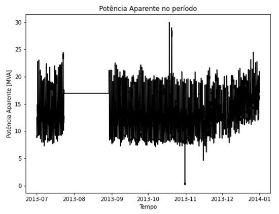
Figure 7.
Apparent power in the period—TR1.
Considering the internal structure of power transformers, the oil temperature is a highly important parameter for the reliable operation of the equipment, as it can intensify degradation mechanisms of the device’s insulating material [2,3,5,34]. In this context, Figure 8 shows the oil temperature of the transformer, taking into account the set of samples available at the time of analysis.
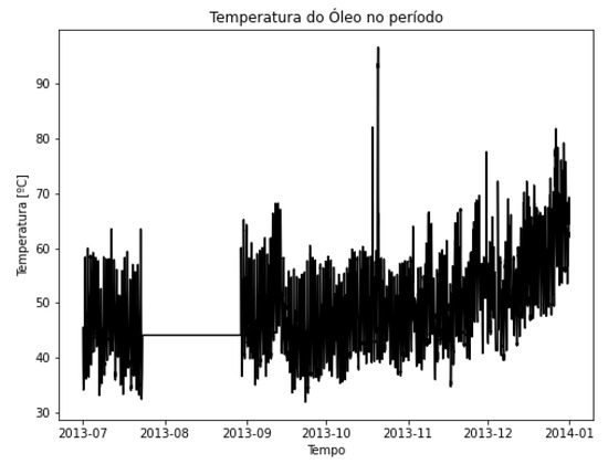
Figure 8.
Oil temperature in the period—TR1.
The analysis of Figure 7 and Figure 8 clearly indicates the presence of failures in data acquisition, where a large gap in the measurements is present. A limitation of current systems is the difficulty in dealing with gaps in operational data in the event of issues with field instrumentation. The proposed methodology can estimate missing data in order to generate realistic operational profiles.
The purpose of the proposed methodology is to track stress mechanisms that can lead to operational failures in the transformer, thereby supporting the maintenance policies of organizations. The environmental operating condition of the transformer is obtained by means of the ambient temperature-estimation model developed and validated in Section 4.1. Figure 9 presents the estimated ambient temperature curve for the location where the equipment is installed.
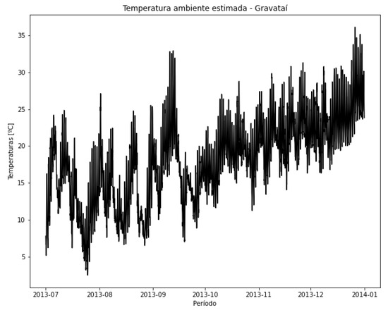
Figure 9.
Estimation of ambient temperature during the period for TR1 locating.
The discrepancy in the data needs to be corrected for subsequent analyses, since the instrumentation failures observed in Figure 7 and Figure 8 reduce the data availability. As a result, the original 17,639 records are reduced to 13,965. The time synchronization between the meteorological vectors and the electrical operational vectors results in 3488 valid synchronous records. The dispersion between the transformer’s oil temperature and the external ambient temperature is shown in Figure 10, where a relationship similar to an exponential curve is observed.
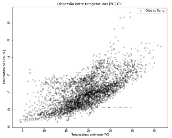
Figure 10.
Dispersion between estimated ambient and oil temperatures—TR1.
Figure 11 complements the analysis by showing the dispersion between the apparent power supplied by the transformer and the ambient temperature. It can be observed from the dispersion results that these quantities are not significant for the transformer load curve.
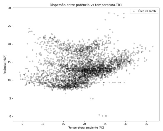
Figure 11.
Dispersion between apparent power and ambient temperature—TR1.
In Figure 12, the oil temperature of transformer TR1 (in red) and the estimated ambient temperature (in blue) are plotted together for comparison. The missing data are only used to synchronize the curves and can be recreated as needed.
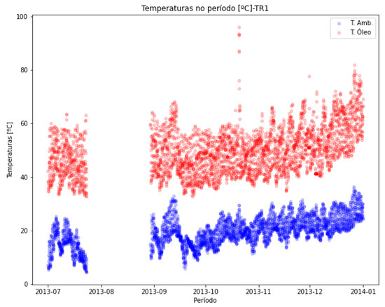
Figure 12.
Estimated ambient temperature and oil temperature—TR1.
The secondary current profile for the transformer can be seen in Figure 13, and a relationship between the transformer oil temperature and its secondary current is shown in Figure 14, where a dependency between the two quantities is indicated.
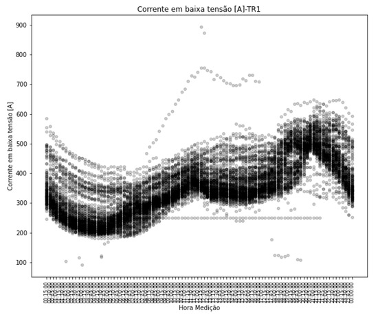
Figure 13.
Secondary current profile—TR1.
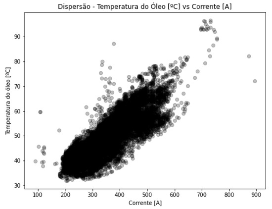
Figure 14.
Dispersion between secondary current and oil temperature—TR1.
Like any electrical machine, power transformers are subjected to heating inherent to the process of transferring power between the primary and secondary windings. The set of post-processed information makes it possible to evaluate the heating profile to which the equipment has been exposed. Thermal stress, in cycles of heating and cooling—considering the daily periods of higher load and ambient temperature—contributes to the activation of failure mechanisms in the transformer, as well as accelerating the aging of its components, especially the insulating paper. Figure 15 shows the oil temperature profile for TR1.
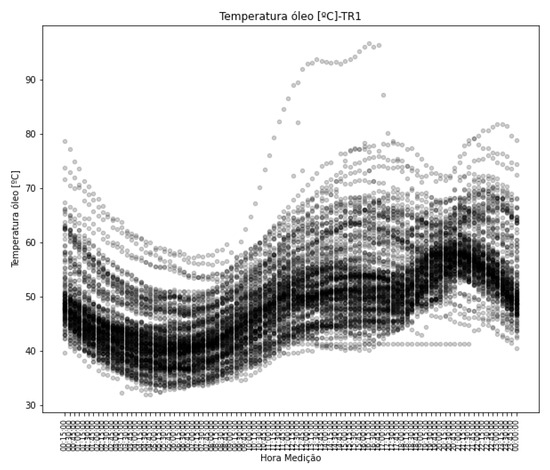
Figure 15.
Oil temperature profile—TR1.
4.2.2. TR2 Transformer Analysis
The application of the methodology for transformer TR2 is presented in this subsection. To avoid making the demonstration excessively long, summarized results are presented. In Figure 16, the power supplied by the transformer during the analysis period from 1 July 2013 to 31 December 2013 is shown, and in Figure 17, the ambient temperature estimation for the same period—reconstructed based on the methodology—is presented.
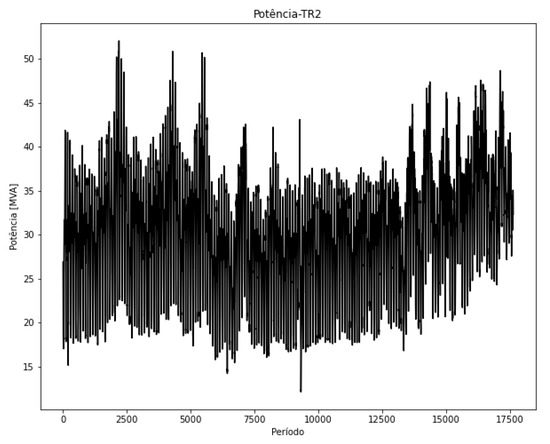
Figure 16.
Apparent power in the period—TR2.
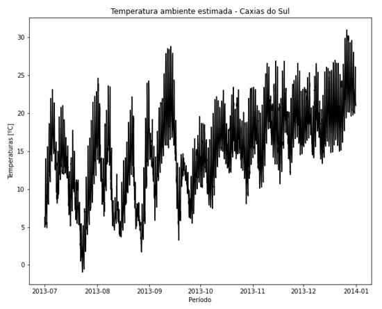
Figure 17.
Estimation of ambient temperature during the period—TR2.
In Figure 18a, the overall profile of supplied power is presented, made possible by the developed analysis methodology. In Figure 18b, the current profile is shown.
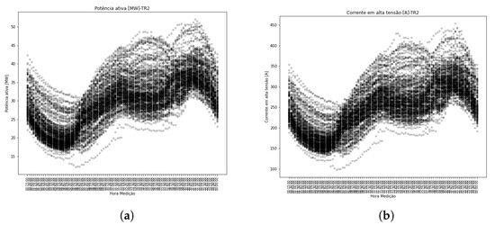
Figure 18.
Power and current profile in the period—TR2. (a) Power profile. (b) Current profile.
In Figure 19a, the top oil temperature for TR2 is presented, along with Figure 19b, which shows the winding temperature. The set of data vectors for transformer TR2 is the only one, among those accessed for this article, that includes both temperatures. An analysis of the temperature profiles can be seen in Figure 20a,b.
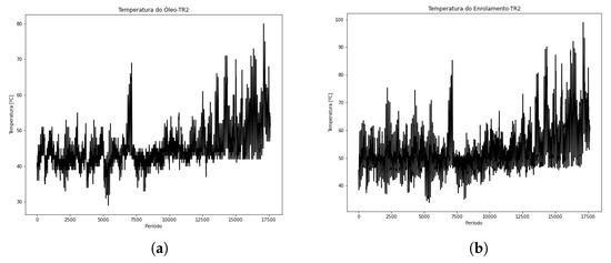
Figure 19.
Oil and winding temperature in the period—TR2. (a) Oil temperature. (b) Winding temperature.
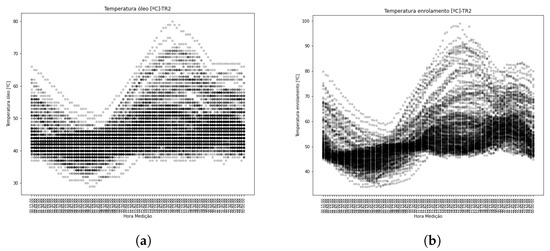
Figure 20.
Temperature profile in the period—TR2. (a) Oil temperature profile. (b) Winding temperature profile.
Based on the methodology, Figure 20a shows the top oil temperature profile of transformer TR2, followed by Figure 20b, which shows the winding temperature profile for the same equipment. Using this information, Figure 21a presents the dispersion between winding temperature and primary current; next, Figure 21b shows the dispersion between top oil temperature and primary current. The correlation between top oil temperature and winding temperature can be seen in Figure 21c.
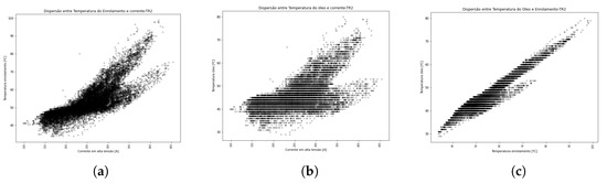
Figure 21.
Dispersion between variables—TR2. (a) vs. corrente. (b) vs. corrente. (c) vs. .
Figure 20b and Figure 21a clearly indicate the temperature variation to which the equipment is subjected over a daily period. The heating and cooling curves of the power transformer illustrate a dynamic behavior, so the use of static or average data can lead to discrepancies in diagnostics. This article contributes a data-processing methodology aimed at improving diagnosis. The stress mechanisms throughout the equipment’s operating lifetime can be tracked and integrated over periods of interest.
Figure 21a–c present the correlations between the variables of top oil temperature, winding temperature, and input current. The linear relationship between top oil temperature and winding temperature is well characterized, indicating the direct possibility of estimating one when the other is measured. Regarding the current, there is a greater concentration of data in the dispersion between winding temperature and current. When relating top oil temperature and current, a greater spread of data is observed, characterizing the influence of the thermal dynamics of the cooling system. Nevertheless, a relationship can be verified, which indicates the possibility of estimating the internal temperatures using only current measurements.
In Figure 22, the winding temperature (in black), the top oil temperature (in red), and the estimated ambient temperature (in blue) are plotted together. Based on these temperatures, a thermal model can be conveniently applied.
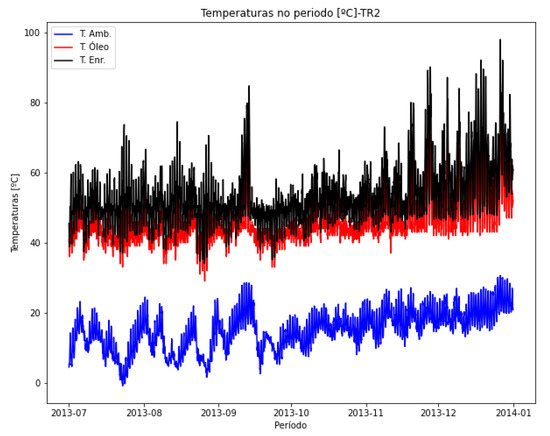
Figure 22.
Estimated ambient, oil and winding temperatures—TR2.
In Figure 23a,b, the dispersions between estimated ambient temperature and oil and winding temperatures are presented. Transformer TR2 operates at a higher load level than TR1 and also includes the measurement of winding temperature. For TR2, the relationship between oil and ambient temperatures generally shows a similarity to the behavior observed in TR1. When analyzing the winding temperature, a relationship close to a quadratic form with positive concavity is indicated.
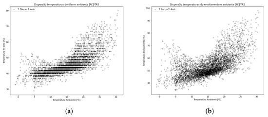
Figure 23.
Dispersion between ambient, oil, and winding temperatures—TR2. (a) vs. . (b) vs. .
4.2.3. TR3 Transformer Analysis
The application of the methodology for transformer TR3 is presented in this subsection. A summarized demonstration is provided in order to keep the article concise. In Figure 24, the power supplied by the transformer during the analysis period from 1 July 2013 to 31 December 2013 is shown; once again, the available data are from this period. In Figure 25, the estimated ambient temperature for the same period, reconstructed based on the methodology, is presented.
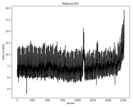
Figure 24.
Apparent power in the period—TR3.
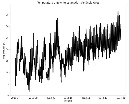
Figure 25.
Estimation of ambient temperature in the period—TR3.
By applying the methodology to transformer TR3, the apparent power profile can be seen in Figure 24, and the secondary current profile is shown in Figure 26b, demonstrating the relationship between these measurements.
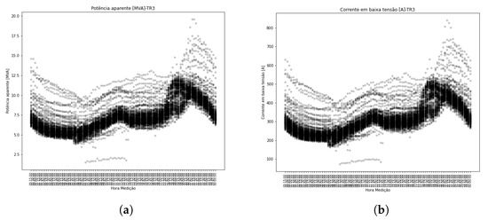
Figure 26.
Power and current profiles in the period—TR3. (a) Power profile. (b) Current profile.
In Figure 27, the top oil temperature is shown, and in Figure 28, its profile is indicated. In this dataset, the winding temperature was not available and, for this reason, it is not presented.
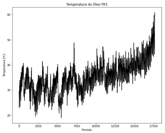
Figure 27.
Oil temperature in the period—TR3.
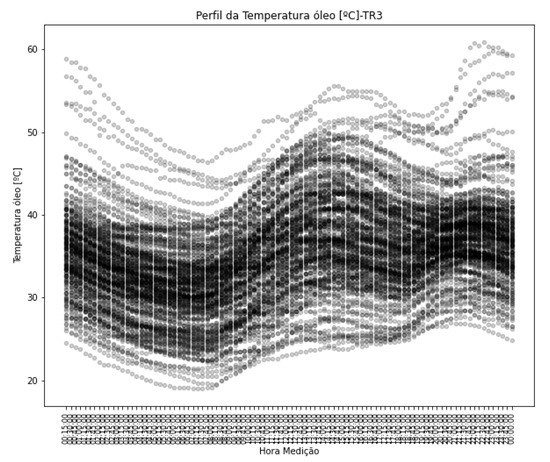
Figure 28.
Oil temperature profile—TR3.
Again, as a way to visualize relationships between different measurements, in Figure 29 the dispersion between top oil temperature and secondary current shows a greater spread of the data, despite a natural trend of increasing temperature as the current increases. Such dispersion results from the thermal characteristics of each transformer, which depend on the design assumptions of their respective manufacturers.
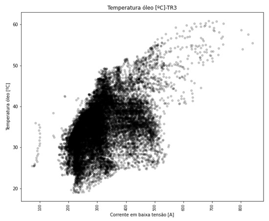
Figure 29.
Dispersion between oil temperature and secondary current—TR3.
In Figure 30, the top oil temperature (in red) and the estimated ambient temperature (in blue) are plotted together for transformer TR3. Figure 31 shows the dispersion between these two quantities. Transformer TR3 is the equipment with the lowest load among those analyzed; as seen in Figure 24, its load exhibits approximately constant behavior, at least during the period for which data are available. These characteristics explain the almost linear relationship between ambient and oil temperature. The equipment operates at comparatively lighter load levels.
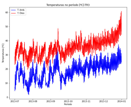
Figure 30.
Estimated ambient temperature and oil temperature—TR3.
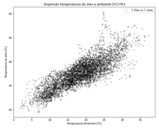
Figure 31.
Dispersion between estimated ambient temperature and oil temperature—TR3.
4.3. Comparison Between Temperature Estimates
Additionally, the developed methodology includes a model that allows estimating ambient temperatures at different locations, based on geographical location and altitude, as well as other input variables. This feature is not explored in related works. Local measurements are not always available, and using distant stations may not accurately reflect local conditions. The use of multiple stations makes it possible to create an arrangement that weights sets of nearby stations.
To facilitate comparison, Figure 32 presents the overlay, on the same axis, of the estimated temperature data vectors for the three locations used. This comparison is qualitative in nature, since there are no actual measured temperature values at the locations.
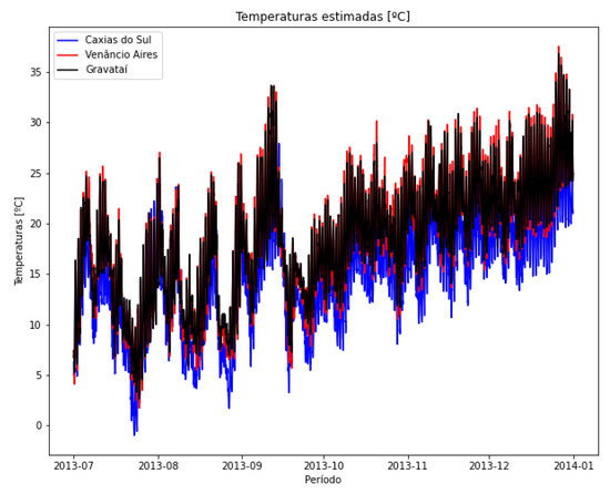
Figure 32.
Comparison between ambient temperature estimation.
4.4. Aging Analysis
With the aim of applying the developed data analysis methodology to verify the equivalent aging of a power transformer, a temperature profile is selected to illustrate the procedure carried out. In Table 5, the data extraction for transformer TR2 is presented, with the day 20 September 2013 arbitrarily chosen to demonstrate the process. Final values are presented for the other transformers to keep the discussion concise.
Table 5.
Equivalent aging on a selected day—TR2.
By applying the data from Table 5 to the equivalent aging model of the IEEE Std C57.91-2011 standard, as previously indicated by Equations (2)–(4), it is possible to evaluate the aging for the suggested day. In Equations (6)–(8), the results are presented. Since the temperatures did not show high gradients in this case, the equivalent aging for the analyzed day can be considered small. Naturally, the cumulative effect should be taken into account.
In Equation (8), the result of represents the percentage aging for the analyzed day for transformer TR2, highlighted here as an example. Based on the IEEE Std C57.91-2011 standard, the suggested service life for the transformer’s insulating material is 180,000 h or 20.54 years. For this lifespan to be achieved, the recommended maximum daily percentage aging is , and in this case, the calculated value is much lower.
In Table 6, the final values of the , , and indicators are presented for the three transformers, based on the available data for the period from 1 July 2013 to 31 December 2013. It is observed that transformer TR2 shows the greatest aging, as it has higher temperatures during the period.
Table 6.
Summary of indicators in the period.
The temporal evolution of for transformer TR1 is presented in Figure 33. The rapid transition in the indicator reflects a specific operating condition in which the equipment supplied a high load.
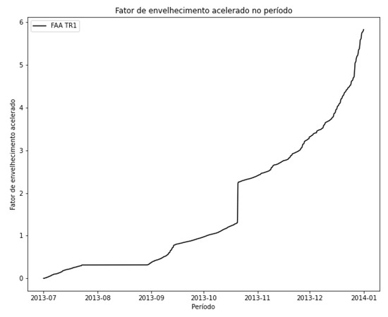
Figure 33.
Evolution of in the period—TR1.
The temporal evolution of for transformer TR2 is presented in Figure 34. Once again, the profile of higher temperatures causes the indicator to show greater increases, especially at the end of the period, which includes the final and typically warmer months of the year.
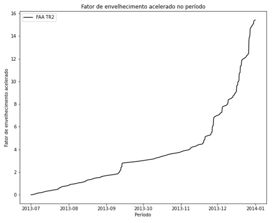
Figure 34.
Evolution of in the period—TR2.
The temporal evolution of for transformer TR3 is presented in Figure 35. Transformer TR3 has the lowest loading among the three, and consequently, its operating temperatures are lower, which mitigates the aging trend. However, a rapid increase in the indicator is again observed during the final months of the year, which is the warmer period.
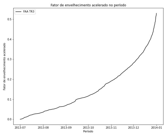
Figure 35.
Evolution of in the period—TR3.
4.5. Detection of Critical Operating Conditions
Power transformers are machines that need to dissipate their heat to the surrounding environment to reduce their temperature. This function is performed by heat exchangers and fans. With changes in ambient temperature, the dissipation capacity is compromised, which can lead to critical operating conditions.
By processing data through the developed methodology, it is possible to detect critical operating conditions that may compromise the equipment’s lifespan. Ambient temperatures above 30 °C are considered in this analysis.
In Figure 36, situations where the ambient temperature exceeds 30 °C (IEEE Std C57.91-2011) are indicated for transformer TR1. The ambient temperature is shown in blue, and the top oil temperature is shown in red, as this is the temperature that needs to be dissipated by the equipment’s cooling system. In the available period, it is observed that differentials of up to 50 °C may occur. Considering that the warmest months of the year are not included in the analyzed period, due to data limitations, it is reasonable to assume that even higher differentials may occur, compromising thermal dissipation. The results for the other transformers are omitted to avoid making the article excessively long.
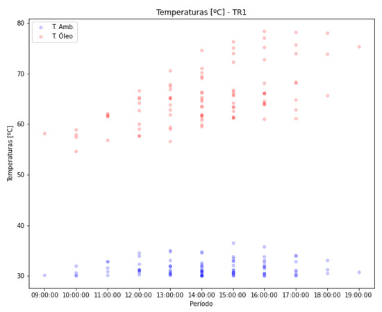
Figure 36.
Temperature difference between and —TR1.
5. Discussion
The proposed methodology enables the creation of operating profiles for the transformer under evaluation, contributing to the planning of preventive maintenance activities. Data correlation makes it possible to understand the behavior of variables and their relationships with other influencing factors. The use of remote data-acquisition technologies is increasingly prominent in the operation and maintenance of power systems, as new technologies facilitate connectivity in remote areas. With large amounts of stored data, data analysis techniques allow for the discovery of correlations between events.
With more accurate information about the transformer’s construction, it is possible to extend the analyses to verify whether operating conditions violate the safe operating limits. Such correlations could enable the creation of a predictive system, indicating the internal wear of its components.
The dataset is not large enough to allow for generalizations of the observed behaviors. The diverse construction characteristics of each transformer make generalization difficult, as different voltage or power levels change the amount of insulation material, volume of insulating oil, and the type of cooling system used. It is suggested that, in the future, transformers be grouped by voltage and power classes.
Transformers TR1 and TR2 show a near-linear relationship between current and top oil temperature; unfortunately, winding temperature measurements are not available to allow for more in-depth analyses. Nevertheless, it is observed that current vector data provide sufficient information to estimate internal temperatures. Considering equipment within the same power and voltage class, this simplification becomes feasible.
The analyses are limited by the availability of records, but the methodology allows verification of the transformer’s current behavior. The use of open-source tools such as Python ensures the method is easily applicable in the operation and planning centers of utility companies, providing predictive maintenance with a new tool capable of indicating equipment aging. This article extends the author’s previous works [6,7,8].
6. Conclusions
The future success of decarbonization ambitions, with the energy transition, undeniably depends on the establishment of asset life management techniques. This work presents technical and scientific contributions that are scarcely explored in the reviewed literature, creating opportunities for further developments. Data must be correctly synchronized so that analysis techniques can be effectively applied and their results considered valid or meaningful. Based on the literature reviewed, relatively little attention has been given to this issue.
Therefore, this article contributes methodologically by proposing an operational data analysis and processing methodology with the potential for global application. Another aspect of methodological contribution is the proposal of a technique for ambient temperature estimation. In the literature, cases were observed where theoretical ambient temperature variation profiles were applied. This implies that the results may not reflect the real characteristics of degradation or capture the actual stress level to which the equipment—in this case, the power transformer—is subjected.
As indicated in the analyses of transformers TR1, TR2, and TR3, the thermal variation cycles exhibit significant amplitude. It is known that such cycles affect the equipment’s power dissipation capacity, as higher ambient temperatures make heat exchange with the external environment more difficult. This creates stress conditions that reduce the device’s service life.
Methodologies such as the Health Index are common practice among electric utilities and other institutions owning power transformers. However, the Health Index will only provide reliable results if it is fed with reliable data. In this sense, failing to consider tangible thermal stress results in unrealistic outcomes. This article contributes in this aspect by estimating thermal profiles for the geographical coordinates of substations. This enables the methodology to be used in remote locations or small installations without advanced monitoring resources, or even in various industrial facilities. A historical thermal profile can thus be developed for the geographic location of interest.
An online system, capturing and processing data in real time, adds substantial advantages in resource management for electricity transmission and distribution companies. Furthermore, equipment manufacturers themselves benefit from the acquired dataset, making transformer designs more robust. The relationship of multiple variables makes it possible to discover stress conditions that were not foreseen or were neglected during equipment design.
This article contributes at different levels and aspects to technical knowledge and the development of the state-of-the-art, highlighting a global methodology for analyzing operational conditions in power transformers, with potential application to other equipment and industrial sectors. Another contribution is a model for estimating ambient temperatures, which can be employed in various areas, including agriculture and livestock applications.
As a suggestion for future work, the application of the methodology could be extended to a larger number of transformers in order to eliminate data bias. In addition, the climate model for ambient temperature estimation could incorporate other measurements such as wind speed, rainfall, and humidity.
Author Contributions
Conceptualization, S.L.; methodology, S.L.; software, S.L.; validation, L.R.P. and P.R.d.S.P.; formal analysis, S.L.; investigation, S.L.; resources, S.L., A.d.R.A., R.M.d.F., L.R.P. and P.R.d.S.P.; data curation, S.L. and A.d.R.A.; writing—original draft preparation, S.L.; writing—review and editing, A.d.R.A., R.M.d.F., L.R.P. and P.R.d.S.P.; visualization, S.L.; supervision, A.d.R.A. and R.M.d.F.; project administration, A.d.R.A. and R.M.d.F.; funding acquisition, R.M.d.F. All authors have read and agreed to the published version of the manuscript.
Funding
This research received no external funding.
Data Availability Statement
The data presented in this study might be available on request from the corresponding author.
Conflicts of Interest
The authors declare no conflicts of interest.
Abbreviations
The following abbreviations are used in this manuscript:
| Aging Acceleration Factor | |
| Equivalent Aging Factor | |
| Percentage loss of insulation life | |
| Ambient temperature | |
| TR | Transformer |
| Oil temperature | |
| Winding temperature |
Appendix A
Table A1.
Coefficients of the linear multiple regression model.
Table A1.
Coefficients of the linear multiple regression model.
| Coefficient | Value |
|---|---|
| X1 | 0.67912297 |
| X2 | −0.28801044 |
| X3 | −0.14481407 |
| X4 | −0.02206486 |
| X5 | 0.59564328 |
| X6 | 0.11723389 |
Table A2.
Parameters of the linear multiple regression model.
Table A2.
Parameters of the linear multiple regression model.
| Parameters | Value |
|---|---|
| Training | 0.378237 |
| Mean squared error | 0.02 |
| Coefficient of determination | 0.39 |
References
- Freitag, S.C.; Sperandio, M.; Marchesan, T.B.; Carraro, R. Failure mode and effect analysis applied to power transformers. In Proceedings of the 2017 52nd International Universities Power Engineering Conference (UPEC), Heraklion, Greece, 28–31 August 2017; pp. 1–6. [Google Scholar] [CrossRef]
- Carraro, R. Desenvolvimento de um “Health Index” Para Transformadores de Potência. Master’s Thesis, Universidade Federal de Santa Maria, Santa Maria, Brazil, 2017. [Google Scholar]
- Freitag, S.C. Análise de Modos e Efeitos de Falhas Aplicado a Transformadores de Potência. Master’s Thesis, Universidade Federal de Santa Maria, Santa Maria, Brazil, 2017. [Google Scholar]
- Freitag, S.C.; Sperandio, M.; Marchesan, T.B.; Carraro, R. Power transformer risk management: Predictive methodology based on reliability centered maintenance. In Proceedings of the 2018 Simposio Brasileiro de Sistemas Eletricos (SBSE), Niteroi, Brazil, 12–16 May 2018; pp. 1–6. [Google Scholar] [CrossRef]
- Feil, D.L.P. Substituíção de Transformadores de Potência em Subestações de Energia: Uma Estratégia Global. Ph.D. Thesis, Universidade Federal de Santa Maria, Santa Maria, Brazil, 2019. [Google Scholar]
- Lessinger, S.; De Figueiredo, R.M.; Prade, L.R.; Da Rosa Abaide, A. Methodology For Operational Analysis Of Power Transformers With Data Science. In Proceedings of the 2021 IEEE PES Innovative Smart Grid Technologies Conference—Latin America (ISGT Latin America), Lima, Peru, 15–17 September 2021; pp. 1–5. [Google Scholar] [CrossRef]
- Lessinger, S.; de Figueiredo, R.M.; Prade, L.R.; da Rosa Abaide, A. Improving Power Transformers Maintenance with Data Science. In Proceedings of the 2021 56th International Universities Power Engineering Conference (UPEC), Middlesbrough, UK, 31 August 2021–3 September 2021; pp. 1–6. [Google Scholar] [CrossRef]
- Lessinger, S.; de Figueiredo, R.M.; Prade, L.R.; da Rosa Abaide, A. Metodologia Para Análise Operacional De Transformadores De Potencia. In Proceedings of the XV Simpósio Brasileiro de Automação Inteligente—SBAI 2021, Rio Grande, Brazil, 17–20 October 2021; Volume 1, pp. 1441–1446. [Google Scholar] [CrossRef]
- Campanhola, F.P. Ferramenta de Apoio à Gestão de Ativos Para Sistema de Potência Empregando os Métodos Ahp e Monte Carlo Aplicada a Transformadores de Potência. Ph.D. Thesis, Universidade Federal de Santa Maria, Santa Maria, Brazil, 2023. [Google Scholar]
- ONS. Análise da Perturbação do dia 03/11/2020 às 20h48min Com Início Nos Transformadores de 230/69/13.8 kv da se Macapá, com Desligamento da Uhe Coaracy Nunes e do Sistema Amapá, 2020. Available online: http://www.ons.org.br/Paginas/Noticias/20201207-ons-divulga-rap-ocorrencia-amapa.aspx (accessed on 15 December 2020).
- Globo. Um Mês do Apagão no Amapá: O que Ainda Precisa para a Segurança Energética? 2020. Available online: https://g1.globo.com/ap/amapa/noticia/2020/12/03/um-mes-do-apagao-no-amapa-o-que-ainda-precisa-para-a-seguranca-energetica.ghtml (accessed on 7 December 2020).
- BBC. Apagão no Amapá: O Que Provocou Queda de Energia Que Leva Sede e caos ao Estado. 2020. Available online: https://www.bbc.com/portuguese/brasil-54843654 (accessed on 3 December 2020).
- ONS. Operação do Segundo Transformador da SE Macapá, 2020. Available online: http://www.ons.org.br/Paginas/Noticias/Operação-do-segundo-transformador-da-SE-Macapá.aspx (accessed on 7 December 2020).
- ONS. Ocorrência no Estado do Amapá—03.11.2020. 2020. Available online: http://www.ons.org.br/Paginas/Noticias/Ocorrência-no-Estado-do-Amapá-03.11.2020.aspx (accessed on 7 December 2020).
- ONS. NOTA 2—Ocorrência no Estado do Amapá—03.11.2020. 2020. Available online: http://www.ons.org.br/Paginas/Noticias/Nota-2-%E2%80%93-Ocorr%C3%AAncia-no-Estado-do-Amap%C3%A1-%E2%80%93-03-11-2020.aspx (accessed on 7 December 2020).
- ANEEL. ANEEL Autoriza Operação de Duas Usinas Termelétricas Para Abastecer o Amapá. 2020. Available online: https://www.aneel.gov.br/sala-de-imprensa-exibicao-2/-/asset_publisher/zXQREz8EVlZ6/content/aneel-autoriza-operacao-de-duas-usinas-termeletricas-para-abastecer-o-amapa/656877? (accessed on 15 December 2020).
- ANEEL. Fiscalização da ANEEL Aplica Multa de R$ 3.6 Milhões na LMTE Por Ocorrência no Amapá. 2020. Available online: https://www.aneel.gov.br/sala-de-imprensa-exibicao-2/-/asset_publisher/zXQREz8EVlZ6/content/fiscalizacao-da-aneel-aplica-multa-de-r-3-6-milhoes-na-lmte-por-ocorrencia-no-amapa/656877? (accessed on 15 December 2020).
- ONS. ONS, CCEE e EPE Divulgam Projeção de Carga Para o Período de 2021 a 2025. 2020. Available online: http://www.ons.org.br/Paginas/Noticias/ONS,-CCEE-e-EPE-divulgam-projecao-de-carga-para-o-periodo-de-2021-a-2025.aspx (accessed on 10 December 2020).
- Cheng, C.K.; Ho, C.T.; Lee, D.; Lin, B. Monolithic 3D Semiconductor Footprint Scaling Exploration Based on VFET Standard Cell Layout Methodology, Design Flow, and EDA Platform. IEEE Access 2022, 10, 65971–65981. [Google Scholar] [CrossRef]
- Prade, L.R. Uma Arquitetura De Comunicação Com Mecanismos Para Atendimento Dos Requisitos Das Redes Elétricas Inteligentes Rurais. Ph.D. Thesis, Universidade Federal de Santa Maria, Santa Maria, Brazil, 2020. [Google Scholar]
- Wanasinghe, T.R.; Gosine, R.G.; James, L.A.; Mann, G.K.I.; de Silva, O.; Warrian, P.J. The Internet of Things in the Oil and Gas Industry: A Systematic Review. IEEE Internet Things J. 2020, 7, 8654–8673. [Google Scholar] [CrossRef]
- Mazon-Olivo, B.; Pan, A. Internet of Things: State-of-the-art, Computing Paradigms and Reference Architectures. IEEE Lat. Am. Trans. 2021, 20, 49–63. [Google Scholar] [CrossRef]
- Keller, A.L. Internet das Coisas Aplicada à Industria: Dispositivo para Interoperabilidade de Redes Industriais. Master’s Thesis, Universidade do Vale do Rio dos Sinos, São Leopoldo, Brazil, 2016. [Google Scholar]
- Haykin, S. Redes Neurais: Princípios e prática; Bookman: Porto Alegre, Brazil, 2001; p. 900. [Google Scholar]
- Muller, A.C.; Guido, S. Introduction to Machine Learning with Python; O’Reilly: Sebastopol, CA, USA, 2017; p. 384. [Google Scholar]
- Abiodun, O.I.; Jantan, A.; Omolara, A.E.; Dada, K.V.; Umar, A.M.; Linus, O.U.; Arshad, H.; Kazaure, A.A.; Gana, U.; Kiru, M.U. Comprehensive Review of Artificial Neural Network Applications to Pattern Recognition. IEEE Access 2019, 7, 158820–158846. [Google Scholar] [CrossRef]
- Chiroma, H.; Abdullahi, U.A.; Abdulhamid, S.M.; Abdulsalam Alarood, A.; Gabralla, L.A.; Rana, N.; Shuib, L.; Targio Hashem, I.A.; Gbenga, D.E.; Abubakar, A.I.; et al. Progress on Artificial Neural Networks for Big Data Analytics: A Survey. IEEE Access 2019, 7, 70535–70551. [Google Scholar] [CrossRef]
- Li, Z.; Liu, F.; Yang, W.; Peng, S.; Zhou, J. A Survey of Convolutional Neural Networks: Analysis, Applications, and Prospects. IEEE Trans. Neural Netw. Learn. Syst. 2021, 33, 6999–7019. [Google Scholar] [CrossRef] [PubMed]
- Figueiredo, R.M.d. Um Sistema Computacional para Previsão de Carga em Sistemas de Energia Elétrica Baseado em Redes Neurais Artificiais. Master’s Thesis, Universidade da Vale do Rio dos Sinos, São Leopoldo, Brazil, 2009. [Google Scholar]
- Evaldt, M.C. Sistema Neural Artificial Para Identificação De Perdas Não Técnicas Em Consumidores Rurais. Ph.D. Thesis, Universidade Federal de Santa Maria, Santa Maria, Brazil, 2018. [Google Scholar]
- Ghunem, R.A.; Assaleh, K.; El-hag, A.H. Artificial neural networks with stepwise regression for predicting transformer oil furan content. IEEE Trans. Dielectr. Electr. Insul. 2012, 19, 414–420. [Google Scholar] [CrossRef]
- Castanheira, L.G.; Vasconcelos, J.A.d.; Reis, A.J.R.; Magalhães, P.H.V.; Silva, S.A.L.d. Application of neural networks in the classification of incipient faults in power transformers: A study of case. In Proceedings of the 2011 International Joint Conference on Neural Networks, San Jose, CA, USA, 31 July–5 August 2011; pp. 3099–3104. [Google Scholar] [CrossRef]
- ENRIQUEZ, A.R.S. Diagnóstico de Falhas em Transformadores de Potência através de Análise de Gases Dissolvidos usando Rede Neural Artificial. Master’s Thesis, Universidade Federal do Maranhão, São Luís, Brazil, 2020. [Google Scholar]
- Kaminski, A.M.; Medeiros, L.H.; Bender, V.C.; Marchesan, T.B.; Oliveira, M.M.; Bueno, D.M.; Neto, J.B.F.; Wilhelm, H.M. Artificial Neural Networks Application for Top Oil Temperature and Loss of Life Prediction in Power Transformers. Electr. Power Components Syst. 2022, 50, 549–560. [Google Scholar] [CrossRef]
- Vianna, E.A.L.; Abaide, A.R.; Canha, L.N.; Miranda, V. Substations SF6 circuit breakers: Reliability evaluation based on equipment condition. Electr. Power Syst. Res. 2016, 142, 36–46. [Google Scholar] [CrossRef]
- Schmitz, W.I.; Feil, D.L.P.; Canha, L.N.; Abaide, A.R.; Marchesan, T.B.; Carraro1, R. Operational vulnerability indicator for prioritization and replacement of power transformers in substation. Int. J. Electr. Power Energy Syst. 2018, 102, 60–70. [Google Scholar] [CrossRef]
- Arias Velásquez, R.M. Health Index for Transformer Condition Assessment. IEEE Lat. Am. Trans. 2019, 16, 2843–2849. [Google Scholar] [CrossRef]
- Murugan, R.; Ramasamy, R. Understanding the power transformer component failures for health index-based maintenance planning in electric utilities. Eng. Fail. Anal. 2019, 96, 274–288. [Google Scholar] [CrossRef]
- Alqudsi, A.; El-Hag, A. Application of Machine Learning in Transformer Health Index Prediction. Energies 2019, 12, 2694. [Google Scholar] [CrossRef]
- Tran, Q.T.; Davies, K.; Roose, L.; Wiriyakitikun, P.; Janjampop, J.; Riva Sanseverino, E.; Zizzo, G. A Review of Health Assessment Techniques for Distribution Transformers in Smart Distribution Grids. Appl. Sci. 2020, 10, 8115. [Google Scholar] [CrossRef]
- Chen, C.; Fu, H.; Zheng, Y.; Tao, F.; Liu, Y. The advance of digital twin for predictive maintenance: The role and function of machine learning. J. Manuf. Syst. 2023, 71, 581–594. [Google Scholar] [CrossRef]
- Oliveira, M.; Medeiros, L.; Kaminski, A.; Falcao, C.; Beltrame, R.; Bender, V.; Marchesan, T.; Marin, M. Thermal-hydraulic model for temperature prediction on oil-directed power transformers. Int. J. Electr. Power Energy Syst. 2023, 151, 109133. [Google Scholar] [CrossRef]
- Balanta, J.Z.; Rivera, S.; Romero, A.A.; Coria, G. Planning and Optimizing the Replacement Strategies of Power Transformers: Literature Review. Energies 2023, 16, 4448. [Google Scholar] [CrossRef]
- Li, S.; Li, X.; Cui, Y.; Li, H. Review of Transformer Health Index from the Perspective of Survivability and Condition Assessment. Electronics 2023, 12, 2407. [Google Scholar] [CrossRef]
- Xing, Z.; He, Y.; Chen, J.; Wang, X.; Du, B. Health evaluation of power transformer using deep learning neural network. Electr. Power Syst. Res. 2023, 215, 109016. [Google Scholar] [CrossRef]
- Zhang, W.; Yang, D.; Wang, H. Data-Driven Methods for Predictive Maintenance of Industrial Equipment: A Survey. IEEE Syst. J. 2019, 13, 2213–2227. [Google Scholar] [CrossRef]
- Marsaro, M.F. Modelos de Manutenção Baseados em Oportunidade Considerando Inspeção Imperfeita e Múltiplos Critérios. Ph.D. Thesis, Universidade Federal de Pernambuco, Recife, Brazil, 2019. [Google Scholar]
- da Silva Fernandes, R. Metodologias Para Determinação de Periodicidade Ótima de Manutenção Preventiva sob a Suposição de Reparo Imperfeito em Manutenção Corretiva. Ph.D. Thesis, Universidade Federal de Minas Gerais, Belo Horizonte, Brazil, 2019. [Google Scholar]
- Alberti, A.R. Modelos Para Apoio à Avaliação de Políticas de Manutenção Para Sistemas de Proteção. Ph.D. Thesis, Universidade Federal de Pernambuco, Recife, Brazil, 2020. [Google Scholar]
- Ribeiro, L.F.A. Desenvolvimento de Modelos de Manutenção Seletiva Integrados a Decisões Orçamentárias e Estratégicas. Ph.D. Thesis, Universidade Federal de Pernambuco, Recife, Brazil, 2021. [Google Scholar]
- Pereira, F.H.; Melani, A.H.d.A.; Kashiwagi, F.N.; Rosa, T.G.d.; Santos, U.S.d.; Souza, G.F.M.d. Imperfect Preventive Maintenance Optimization with Variable Age Reduction Factor and Independent Intervention Level. Appl. Sci. 2023, 13, 10210. [Google Scholar] [CrossRef]
- Yang, J.; Wu, H.; Yang, Y.; Zhao, X.; Xun, H.; Wei, X.; Guo, Z. A Transformer Maintenance Interval Optimization Method Considering Imperfect Maintenance and Dynamic Maintenance Costs. Appl. Sci. 2024, 14, 6845. [Google Scholar] [CrossRef]
- Breznická, A.; Kohutiar, M.; Krbat’a, M.; Eckert, M.; Mikus, P. Reliability Analysis during the Life Cycle of a Technical System and the Monitoring of Reliability Properties. Systems 2023, 11, 556. [Google Scholar] [CrossRef]
- Osara, J.A.; Bryant, M.D. Systems and Methods for Transformation and Degradation Analysis. Entropy 2024, 26, 454. [Google Scholar] [CrossRef] [PubMed]
- Simões, M.G.; Farret, F.A.; Khajeh, H.; Shahparasti, M.; Laaksonen, H. Future Renewable Energy Communities Based Flexible Power Systems. Appl. Sci. 2022, 12, 121. [Google Scholar] [CrossRef]
- Pereira, F.H.; Bezerra, F.E.; Junior, S.; Santos, J.; Chabu, I.; Souza, G.F.M.d.; Micerino, F.; Nabeta, S.I. Nonlinear Autoregressive Neural Network Models for Prediction of Transformer Oil-Dissolved Gas Concentrations. Energies 2018, 11, 1691. [Google Scholar] [CrossRef]
- Dong, M.; Zheng, H.; Zhang, Y.; Shi, K.; Yao, S.; Kou, X.; Ding, G.; Guo, L. A Novel Maintenance Decision Making Model of Power Transformers Based on Reliability and Economy Assessment. IEEE Access 2019, 7, 28778–28790. [Google Scholar] [CrossRef]
- Huang, W.; Li, X.; Hu, B.; Yan, J.; Peng, L.; Sun, Y.; Cheng, X.; Ding, J.; Xie, K.; Liao, Q.; et al. A Data Mining Approach for Transformer Failure Rate Modeling Based on Daily Oil Chromatographic Data. IEEE Access 2020, 8, 174009–174022. [Google Scholar] [CrossRef]
- Foros, J.; Istad, M. Health Index, Risk and Remaining Lifetime Estimation of Power Transformers. IEEE Trans. Power Deliv. 2020, 35, 2612–2620. [Google Scholar] [CrossRef]
- Fauzi, N.A.; Ali, N.H.N.; Ker, P.J.; Thiviyanathan, V.A.; Leong, Y.S.; Sabry, A.H.; Jamaludin, M.Z.B.; Lo, C.K.; Mun, L.H. Fault Prediction for Power Transformer Using Optical Spectrum of Transformer Oil and Data Mining Analysis. IEEE Access 2020, 8, 136374–136381. [Google Scholar] [CrossRef]
- Ferreira Dias, C.; de Oliveira, J.R.; de Mendonça, L.D.; de Almeida, L.M.; de Lima, E.R.; Wanner, L. An IoT-Based System for Monitoring the Health of Guyed Towers in Overhead Power Lines. Sensors 2021, 21, 6173. [Google Scholar] [CrossRef] [PubMed]
- Chen, X.; Hu, Y.; Dong, Z.; Zheng, P.; Wei, J. Transformer Operating State Monitoring System Based on Wireless Sensor Networks. IEEE Sens. J. 2021, 21, 25098–25105. [Google Scholar] [CrossRef]
- Freitag, S.C.; Sperandio, M. A modeling and simulation framework for composite reliability assessment considering adverse weather conditions. Electr. Power Syst. Res. 2022, 208, 107915. [Google Scholar] [CrossRef]
- Franco, I.T.; de Figueiredo, R.M. Predictive Maintenance: An Embedded System Approach. J. Control. Autom. Electr. Syst. 2022, 34, 2195–3899. [Google Scholar] [CrossRef]
- Python. Python Programming Language. 2021. Available online: https://www.python.org/ (accessed on 10 February 2021).
- Pandas. Data Structures for Statistical Computing in Python. 2021. Available online: https://pandas.pydata.org/pandas-docs/stable/ (accessed on 12 February 2021).
- Matplotlib. Matplotlib: Visualization with Python, 2021. Available online: https://matplotlib.org/ (accessed on 12 February 2021).
- IEEE Std C57.91-2011; IEEE Guide for Loading Mineral-Oil-Immersed Transformers and Step-Voltage Regulators. The Institute of Electrical and Electronics Engineers: New York, NY, USA, 2011.
Disclaimer/Publisher’s Note: The statements, opinions and data contained in all publications are solely those of the individual author(s) and contributor(s) and not of MDPI and/or the editor(s). MDPI and/or the editor(s) disclaim responsibility for any injury to people or property resulting from any ideas, methods, instructions or products referred to in the content. |
© 2025 by the authors. Licensee MDPI, Basel, Switzerland. This article is an open access article distributed under the terms and conditions of the Creative Commons Attribution (CC BY) license (https://creativecommons.org/licenses/by/4.0/).