Effects of Electricity Price Volatility, Energy Mix and Training Interval on Prediction Accuracy: An Investigation of Adaptive and Static Regression Models for Germany, France and the Czech Republic

Abstract

Electricity markets in Europe have undergone major changes in the last decade, mainly due to the increasing share of variable renewable energy sources (RES), changing demand patterns, and geopolitical factors—particularly the war in Ukraine, tensions over energy imports, and disruptions in natural gas supplies. These changes have led to increased electricity price volatility, reducing the reliability of traditional forecasting tools. This research analyses the potential of static and adaptive linear regression as electricity price forecasting tools in the context of three countries with different energy mixes: Germany, France and the Czech Republic. The static regression approach was compared with an adaptive approach based on incremental model updates at monthly intervals. Testing was carried out in three different scenarios combining stable and turbulent market periods. The quantitative results showed that the adaptive model achieved a lower MAE and RMSE, especially when trained on data from high-volatility periods. However, models trained under turbulent conditions performed poorly in stable environments due to a shift in market dynamics. The results supported several of the hypotheses formulated and demonstrated the need for localised, flexible and continuously updated forecasting. Limitations of the adaptive approach and suggestions for future research, including changing the length of training windows and the use of seasonal models, are also discussed. The research confirms that modern markets require adaptive analytical approaches that account for changing RES dynamics and country specificities.

1. Introduction

Over the past decade, the European Union has significantly accelerated the deployment of renewable energy sources (RES), particularly wind and solar power, as part of its climate policy aimed at reducing greenhouse gas emissions and strengthening energy independence. While this transition contributes to decarbonization, it also introduces new challenges—especially the increased volatility of electricity prices caused by weather dependency, seasonal fluctuations in generation, and limited energy storage options. One visible consequence of these dynamics is the occurrence of negative electricity prices, which typically arise when RES production exceeds demand and the system lacks sufficient flexibility. The frequency of these price extremes has been increasing in parallel with the growing share of RES, particularly in countries such as Germany, Denmark, Spain, and the Netherlands. This growing volatility undermines market stability, complicates production planning, and affects investor confidence. As electricity systems become more dynamic, traditional forecasting models based on fixed historical periods often fail to respond adequately. Therefore, it is increasingly urgent to employ advanced modelling approaches capable of adaptively reacting to changing market conditions and more accurately capturing the impact of RES on electricity price development [1,2,3,4].

High dependence on weather conditions, generation seasonality, and limited electricity storage capacity are among the main drivers of increasingly frequent price fluctuations. Several studies confirm that insufficient battery or grid-scale storage hinders effective balancing between generation and consumption, thereby negatively affecting market stability and production planning [5,6].

The increasing share of renewables, in particular variable forms such as wind and photovoltaics, is also reflected in the price development in the most important European electricity market—Germany. The following table (

Table 1. Average monthly electricity prices in Germany between 2015 and 2025.

	2015	2016	2017	2018	2019	2020	2021	2022	2023	2024	2025
1	27.05	29.01	52.56	30.49	50.24	34.52	53.05	169.99	120.35	78.51	119.28
2	36.67	22.01	39.63	40.17	42.74	21.68	48.54	131.37	130.13	61.29	127.89
3	31.38	24.31	31.69	37.26	30.52	23.02	47.19	249.64	99.63	63.35	93.53
4	29.75	24.20	28.28	31.58	36.79	16.63	53.76	166.70	101.84	61.35	76.33
5	25.34	22.56	31.05	34.31	37.80	17.59	53.61	178.11	81.22	69.03	67.20
6	30.09	27.71	29.98	42.13	32.64	26.84	74.65	220.97	94.45	87.18	62.29
7	34.99	27.18	33.02	49.87	39.79	29.96	80.55	318.25	78.12	67.83
8	31.61	27.18	30.88	56.28	36.63	35.35	84.06	469.79	95.29	80.99
9	31.89	30.52	34.23	54.95	35.99	43.52	128.09	330.74	99.55	78.57
10	39.35	37.16	28.47	52.79	36.85	33.46	139.33	152.12	86.84	86.40
11	32.36	38.08	40.63	56.78	41.18	39.69	176.31	184.48	94.59	114.35
12	27.80	37.49	29.50	47.30	31.80	43.37	220.69	239.38	63.69	104.93

) illustrates the average monthly electricity prices in Germany between 2015 and 2025.

From Table 1, it can be seen that the period from 2015 to 2019 was characterised by relatively stable and low electricity prices, which were in the range of around 25 to 55 €/MWh in the vast majority of months. This corresponded with a lower share of variable RES in the market and more stable market conditions.

A significant change occurred after 2020, when sharp price increases could be observed, especially in months with a higher share of wind and solar generation or in the context of external factors such as global energy shocks, rising fuel prices or reduced availability of conventional resources. The peak of this trend was in 2022, when in some months (e.g., August 2022) the average electricity price reached extremes above 400 €/MWh.

Data for 2023 to 2025 indicate a partial stabilisation of the market, but price levels remain elevated and volatile compared to the previous period, confirming the continued market volatility caused by a combination of the growing share of RES and changing geopolitical and economic conditions. This situation highlights the need to develop new analytical tools to allow more accurate electricity price forecasting and a better understanding of the links between the share of renewables and market dynamics.

2. Overview of the Current State of Knowledge and the Impact of RES on Market Dynamics

In line with the Paris Agreement and the EU’s climate ambitions, member states have significantly accelerated their efforts to decarbonise the energy sector. A central tool in achieving these targets is the increasing share of renewable energy sources (RES), particularly wind and solar, in national electricity mixes. The European Green Deal aims to make Europe climate neutral by 2050 [1], while the Fit for 55 legislative package sets a target of at least a 55% reduction in greenhouse gas emissions by 2030 [2]. According to RED II/III, the share of RES in final energy consumption should reach at least 42.5% by 2030, with the potential to reach 45% [3].

While these policies represent a major step forward, they place growing demands on market flexibility, infrastructure, and cross-border cooperation. The variability of RES, strongly dependent on meteorological conditions, has introduced new challenges for electricity markets. Increased fluctuations in production have led to greater price volatility, complicating system planning and decreasing market stability [4,5,6].

The COVID-19 pandemic, geopolitical tensions, and the energy crisis have further exposed the vulnerability of traditional forecasting tools. This context underscores the need for dynamic, responsive prediction models capable of operating under high volatility and structural change [4].

Studies confirm that as the share of variable RES increases, price fluctuations increase, price extremes, including negative prices, become more frequent, and the predictability of prices in short-term markets decreases [7,8]. This phenomenon is particularly pronounced in markets with a high proportion of wind and sun, such as Germany, Denmark, Spain or the Netherlands.

According to IRENA [7], wind and solar dominate new RES installations in Europe, and their output can at times cover a large portion of electricity demand [8]. This intermittency often causes oversupply, which depresses market prices—occasionally pushing them into negative territory. Conversely, during low RES output combined with high demand, electricity prices may spike dramatically, threatening market stability.

However, the impacts of RES on the price level are not always clear-cut. While some studies show a decrease in the average electricity price as the share of RES increases, known as the merit-order effect—where renewable sources with zero or near-zero marginal costs displace more expensive conventional generators—others point to an increase in volatility and risks for market participants. The magnitude of the merit-order effect varies across systems and depends on the level of RES penetration, market design, flexibility mechanisms, and the availability of storage and interconnections [7,9,10].

Understanding how variable RES—particularly wind and solar—affect price dynamics is critical. Negative prices have become increasingly frequent in countries with high RES penetration, including Germany, the Netherlands, and Denmark [11,12]. These events typically occur during low demand periods (e.g., weekends, holidays), when high RES output coincides with limited export or storage capacity [13].

This study addresses these phenomena by analysing the link between RES-induced volatility and electricity price prediction accuracy, using adaptive regression models.

According to ENTSO-E data and analyses by international institutions, a record number of hours with negative electricity prices were recorded in both Germany and the Netherlands in 2023 [14]. In Germany, for example, the number of such hours exceeded 300, an all-time high.

The occurrence of negative electricity prices has a number of implications for the functioning of the market:

-

Market distortions and investment risk: Long-term and frequent negative prices reduce the return on investment in conventional and flexible resources, which can paradoxically jeopardise the stability of the grid [15].

-

Increased flexibility requirements: The continued inability of the grid to respond flexibly to fluctuations in RES generation increases the importance of technologies such as battery storage, demand-side management or cross-border interconnections [16].

-

Complications in forecasting and planning: Uncertainty caused by extreme price fluctuations, including negative prices, complicates market forecasting, increasing the risk for traders and system operators [17].

The increased frequency of negative prices is considered as one indicator that the current market design is not fully adapted to the reality of a high share of variable RES. This study therefore investigates the link between RES share and price extremes, including negative prices, in order to provide insights for more efficient prediction models and market solutions.

Many existing scientific studies in the last decade have focused on quantifying the impact of RES on average electricity prices or on analysing price volatility related to RES integration. However, most of these works use static models that are based on historical data of a fixed time period. These models assume invariance of market relationships, which is questionable in an environment of a dynamically changing energy sector and increasing RES integration. In an environment where market conditions are influenced by new external factors such as geopolitical shocks (war in Ukraine), energy crises, accelerated decarbonisation or technological developments, more flexible, so-called adaptive approaches to electricity price analysis and forecasting are necessary. Adaptive analytical approaches, which continuously update model parameters according to new data, are now increasingly discussed in the academic community. They allow capturing the changing relationships between RES share, market mechanisms and price dynamics and thus increase the accuracy of the prediction, especially in the short term [18,19,20,21].

To strengthen the methodological context and highlight the relevance of adaptive modelling approaches, several recent studies leveraging deep learning and ensemble methods have been considered. In [22] is developed multiple deep learning models for the Spanish market, including convolutional and recurrent neural networks, emphasising the ability of CNNs to outperform baseline methods in short-term price forecasting. Han and Wang [23] proposed a hybrid Transformer–GNN model (TransGraph-Opt) that jointly captures temporal and spatial dependencies, showing superior performance compared to traditional ML approaches, particularly in large-scale markets. Ghimire et al. [24] introduced a dual-decomposition deep hybrid model capable of handling exogenous variables like weather and demand features, thus enhancing generalisation under volatile market regimes. Similarly, Tian et al. [25] combined local marginal price and extended LMP modelling in an ensemble deep learning framework, achieving notable improvements in predictive accuracy and model stability. These studies demonstrate the evolution of electricity price forecasting from classical statistical models to data-driven, multimodal architectures.

While the present study focuses on linear adaptive modelling to ensure interpretability and computational simplicity, future research may incorporate comparative benchmarks involving ensemble methods and deep architectures, particularly in high-volatility regimes. Furthermore, expanding the dataset beyond the European context could help assess the generalizability of findings across different market structures.

3. Research Objectives and Methodology

The dynamic evolution of electricity markets in Europe in the context of the increasing share of renewables, in particular wind and solar, brings new challenges in electricity price forecasting and understanding market volatility. Classical forecasting models, which use historical data from a fixed period, may lack flexibility and accuracy in such a rapidly changing environment. The research described in this paper responds to these challenges by designing and implementing an adaptive regression model that allows for continuous updating of the relationship between the share of production from RECs and price dynamics. The model “learns” from new data in real time, thereby reflecting current market conditions and improving the accuracy of short- and medium-term electricity price forecasting. At the same time, the research focuses on a comparative analysis between several European countries that differ in their level of RES integration, generation mix and grid flexibility—namely Germany, the Czech Republic and France. This approach allows for a better understanding of how the impacts of variable RES on market stability vary depending on local specificities. The aim of this chapter is to present the methodological framework of the research, including the definition of the analytical objectives, the characterisation of the data used, the description of the models and the methods for assessing the prediction accuracy.

3.1. A More Precise Definition of the Main and Sub-Objectives

The main scientific objective of this study is to evaluate the effectiveness of using an adaptive regression model to predict electricity prices in an environment with an increasing share of renewable energy sources, in particular wind and solar power plants. In the context of increasing market volatility, the study focuses on comparing the predictive accuracy of adaptive and classical static regression approaches.

Part of the main objective is to identify differences in the impact of RES share on price level, volatility and the occurrence of price outliers in different European countries with different energy mix structures and system flexibility.

In addition to the main scientific contribution, the study also pursues practical and applied sub-objectives:

-

To quantify the impact of the share of wind and solar generation on the average electricity price in the analysed countries.

-

To investigate the relationship between the share of variable RES and the occurrence of negative electricity prices as an indicator of market instability.

-

Verify the ability of the adaptive model to capture changing market relationships in real time and to adapt predictions to current conditions.

-

To propose a methodological approach that can be used by practical users (e.g., system operators, electricity traders) without the need for sophisticated software, using only MS Excel and VBA tools.

The research should determine whether adaptive modelling provides better prediction results, especially in a high-volatility environment after 2020, and whether differences between markets affect the relationship between RES share and price dynamics.

3.2. Data Characteristics, RES Share Calculations and Hypothesis Design

The analysis in this paper is based on historical data on electricity generation from individual sources, total consumption and electricity price developments in short-term markets. The data used come from publicly available databases, in particular the ENTSO-E Transparency Platform, which provides hourly and daily data on electricity generation by source, including wind and PV, as well as the market platforms EPEX SPOT and Nord Pool, which provide historical price data. Additional information on electricity production and consumption patterns was obtained from Eurostat statistics and national regulatory authorities.

The time span of the data covers the period 2015 to 2025. This period is purposely divided into three analytical segments. The first segment covers the years 2015 to 2019, which are considered to be a phase of relatively lower volatility and a lower share of variable renewables. The second segment covers the years 2020 to 2023, which are characterised by increased market volatility, an increasing share of RES and an increased frequency of price outliers. The third segment, covering the years 2024 and 2025, is designed to validate the predictive accuracy of the models on independent data (out-of-sample testing).

For comparability between different countries, it is necessary to express the impact of renewables in terms of their share of total electricity generation or consumption. Therefore, the share of wind and solar generation in % is calculated from the available data—aggregated daily data from hourly data. The shares will be calculated by a simple formula:

$$P_{solar+wind}={\displaystyle \frac{P_{solar}+P_{wind}}{P_{total}}}\times 100\%$$

(1)

where P_solar+wind is the absolute electricity generation from wind and PV P_total is the total electricity generation or consumption in a given time period, assuming that generation approximately replicates consumption under normal operating conditions. The use of percentages allows a fair comparison between countries with different market size and consumption.

An important part of the analysis is to examine price volatility and the occurrence of electricity price outliers. Price volatility in this research will be expressed through the standard deviation of prices in monthly or daily aggregations, thus quantifying the dispersion of prices around the mean over a defined period. Two situations will be considered as price outliers: negative prices, i.e., an electricity price below 0 €/MWh, and high price outliers whose occurrence exceeds a predefined threshold level (e.g., 200 €/MWh), which will be defined on the basis of the historical evolution and characteristics of the market in question. Based on the research objectives, the following hypotheses were formulated and will be tested in the analytical part of the study—see

Table 2. Description of the hypotheses addressed in the research.

Hypothesis	Hypothesis Formulation	Expected Relationship or Outcome
H1	The adaptive regression model will achieve lower prediction error (MAE, RMSE) compared to the static model	Adaptive model will be more accurate
H2	The accuracy of the adaptive regression model will be higher in the high-volatility period (2020–2023) compared to the low volatility period (2015–2019)	Adaptive method is more responsive to turbulent market conditions
H3	Regression models trained in periods of high volatility exhibit lower predictive accuracy when applied to stable market conditions.	A model from a turbulent period does not transfer well to a stable environment.
H4	Adaptive regression significantly reduces prediction error even when the model is trained on stable market conditions and applied to periods of high volatility.	Adaptive updating should compensate for the inappropriateness of the original training period.
H5	Regression models trained in a stable period exhibit lower predictive accuracy when applied to periods of high volatility.	A model from a low volatility period is not suitable for a turbulent environment.

.

Testing these hypotheses will allow for a comprehensive assessment of not only the adaptive model’s ability to predict electricity prices, but also its flexibility and sensitivity to changing market conditions.

3.3. Adaptive and Static Regression Models

Regression analysis is a standard tool for quantifying the relationship between independent variables and the dependent variable under study. In the context of this study, regression models are used to capture the relationship between the share of generation from variable renewables, specifically aggregate generation from wind and solar, and electricity price dynamics in short-term markets.

The traditional approach, referred to as static regression, relies on modelling the relationship based on historical data of a fixed period. The parameters of the model are determined once based on the input data, assuming that these parameters are stable and do not change even if market conditions evolve. The static model in this study takes the following form:

$${PRICE}_t=\alpha +\beta \times P_{solar+wind}$$

(2)

where PRICE_(t) is the price of electricity at time t, P_solar+wind is the share of generation from wind and solar combined in total generation at time t (in %), and α, β are regression coefficients estimated from the sample data. The model results in a predicted electricity price value for each time point based on the known share of generation from RES. The static model allows the evaluation of the relationship between the RES share and the electricity price, but in an electricity market environment where conditions fluctuate rapidly due to RES growth, seasonality, external shocks or technological developments, its predictive ability may be limited.

To overcome these limitations, this research implements an adaptive (stepwise) regression model that is continuously updated as new data is added. This approach allows the model to continuously “learn” from current market conditions and adjust its parameters to reflect the changing relationship between the share of variable RES and price dynamics. The adaptive model works in several steps:

• First, a regression model is built based on an initial time period (e.g., years 2015–2017).
• After each new month, a new observation is added to the training dataset, the model is re-estimated, and its parameters are updated. This monthly update interval was chosen to align with the structure of available data and to ensure the model responds appropriately to market changes without being overly reactive.
• This process continues throughout the analysis, with the model reflecting the latest data and market developments in real time.

The adaptive approach has the advantage of greater flexibility and responsiveness to changing market conditions, such as rapid increases in RES share, changes in demand, price fluctuations or external factors. The adaptive model thus provides more realistic predictions, especially in a turbulent market environment. This approach allows for continuous data updates and automatic model updates. The difference between the predicted and actual electricity price is evaluated for each time point as:

$$DIFF={PRICE}_{real}-{PRICE}_{predict}$$

(3)

where PRICE_real is the real price at time t and PRICE_predict is the predicted price based on the regression.

To evaluate the added value of the adaptive regression model, we benchmark its performance against a traditional static linear regression model. The static model, estimated on a fixed historical window without periodic updates, serves as a baseline for comparison across all scenarios. This approach enables us to assess the benefits of model adaptivity under varying market conditions and training intervals.

3.4. Evaluation of the Prediction Accuracy of the Models

The accuracy of the regression models used to predict electricity prices is evaluated in this study by two basic steps. In the first step, for each time point, the individual prediction error is calculated as the difference between the actual and modelled electricity price value according to the formula:

$${DIFF}_t={PRICE}_t^{real}-{PRICE}_t^{predict}$$

(4)

where ${PRICE}_t^{real}$ is the actual observed electricity price at time t, ${PRICE}_t^{predict}$ is the electricity price calculated using the regression model. electricity price calculated using the regression model. These individual errors are then used in a second step to quantify the overall accuracy of the models over the entire period of analysis. Two standard metrics are calculated for this purpose:

• Mean Absolute Error (MAE):

$$MAE={\displaystyle \frac{1}{n}}{\sum }_{t=1}^n\left({PRICE}_t^{real}-{PRICE}_t^{predict}\right)$$

(5)

2.

Root Mean Squared Error (RMSE):

$$RMSE=\sqrt{{\displaystyle \frac{1}{n}}{\sum }_{t=1}^n{\left({PRICE}_t^{real}-{PRICE}_t^{predict}\right)}^2}$$

(6)

where n is the number of time points (data observations) over the period analysed. The MAE indicator expresses the average magnitude of the absolute prediction error, being uniformly sensitive to all outliers regardless of their direction. The RMSE takes into account the squared errors, thus penalising larger deviations more heavily and providing information on how significantly individual predictions differ from reality. Comparing the MAE and RMSE values between the static and adaptive regression models will allow an objective assessment of whether the adaptive model provides more accurate electricity price prediction results, which is the basis for testing the main research hypothesis of this research.

4. Research Results of the Static Regression Model

In this section of the paper, static regression models were applied to evaluate the extent to which electricity price can be predicted based on the historical relationship between the share of wind and solar generation in total generation and the price in short-term markets. The static approach assumes that the relationship between the variables analysed is stable over time, while the parameters of the regression model remain unchanged during the forecast period.

In order to test the model comprehensively, three scenarios have been proposed which take into account different market conditions at different points in time. The choice of these scenarios is based on the characteristics of the evolution of the European electricity markets in recent years, in particular the growing share of renewables, the increasing volatility of prices and the subsequent efforts to stabilise the market.

Scenario 1: Training data 2015–2019, forecast period 2020–2025

This scenario simulates a situation in which the regression model is built based on historical data from a period of relatively lower volatility and more stable market conditions prior to 2020. The model is then used to forecast electricity prices in a period characterised by increased market volatility, more frequent price outliers, and an increasing share of RECs. The objective of this scenario is to see if the model is able to capture the turbulent period 2020 to 2025 under steady-state conditions.

Scenario 2: Training data 2020–2023, forecast period 2024–2025

In the second scenario, the regression model is built based on data from 2020 to 2023, which were marked by high price volatility, an increase in the share of variable RECs and the impact of external fundamentals. The model is then used to forecast for the years 2024 and 2025, which may represent a phase of market stabilisation, partly influenced by the implementation of flexibility measures such as energy storage or improved system management. This scenario verifies that a model trained in difficult market conditions remains reliable even when moving into a calmer period.

Scenario 3: Training data 2020–2025, forecast period 2015–2019 (model simulation)

The third scenario is specific, as in this case the regression model is built on data from 2020 to 2025, a period of high volatility, and then back-tested on data from 2015 to 2019. Although this is a model situation, this scenario is designed to simulate a possible future situation in which the market would reach a stabilisation, similar to the pre-2020 period, after a period of high volatility. Such a development could occur due to the implementation of large-scale storage, improved grid flexibility or advanced demand management. The scenario thus allows to verify whether a model trained in turbulent conditions is able to capture price dynamics in a more stable environment.

Each of the scenarios was applied separately for selected European countries with different energy mix structure and RES share, namely Germany (GE), France (FR) and Czech Republic (CZ). The results of the models are presented in the form of regression equations, a graphical comparison of actual and modelled electricity prices, as well as a quantitative evaluation of the prediction accuracy through MAE and RMSE indicators.

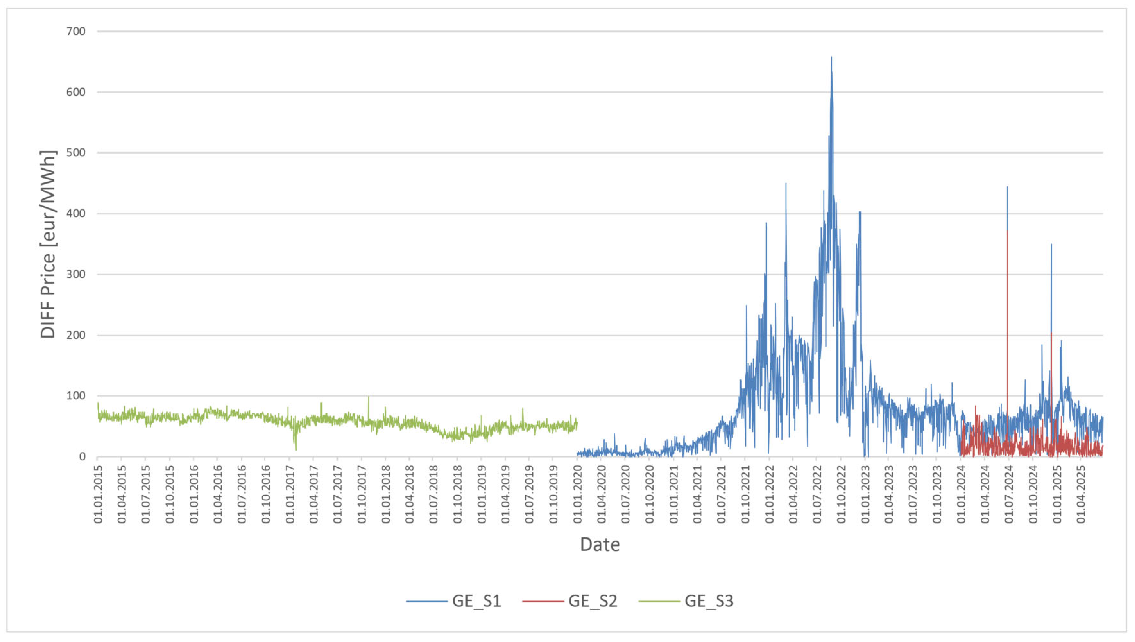
4.1. Research Results of the Static Regression Model for Germany—Figure 1

For Germany the following regression equations were obtained:

Scenario 1: Training data 2015–2019→ prediction 2020–2025

Equation: y = −0.5933 ∗ x + 49.9936

Scenario 2: Training data 2020–2023→ prediction 2024–2025

Equation: y = −2.5746 ∗ x + 207.2316

Scenario 3: Training data 2020–2025→ backcast 2015–2019

Equation: y = −0.3282 ∗ x + 80.2483

In the case of Germany (Figure 1), scenario S1 (curve GE_S1), which uses the period 2015–2019 as the training set, experienced significant prediction errors during years with extremely volatile price developments (especially 2021–2022). The DIFF Price curve oscillates significantly and peaks at over €600/MWh, indicating that the model trained on a stable period is not able to capture market shocks. In scenario S2 (training: 2020–2023, forecast: 2024–2025), the errors are significantly lower (GE_S2 curve), the forecasts are close to the real prices, indicating a better adaptability of the model to similar volatile conditions. Scenario S3 (training: 2020–2025, forecast: 2015–2019) shows a relatively stable path (curve GE_S3) with lower errors, but slightly overestimates the price level in certain periods, which may be due to extrapolation from a volatile period to a historically calm market.

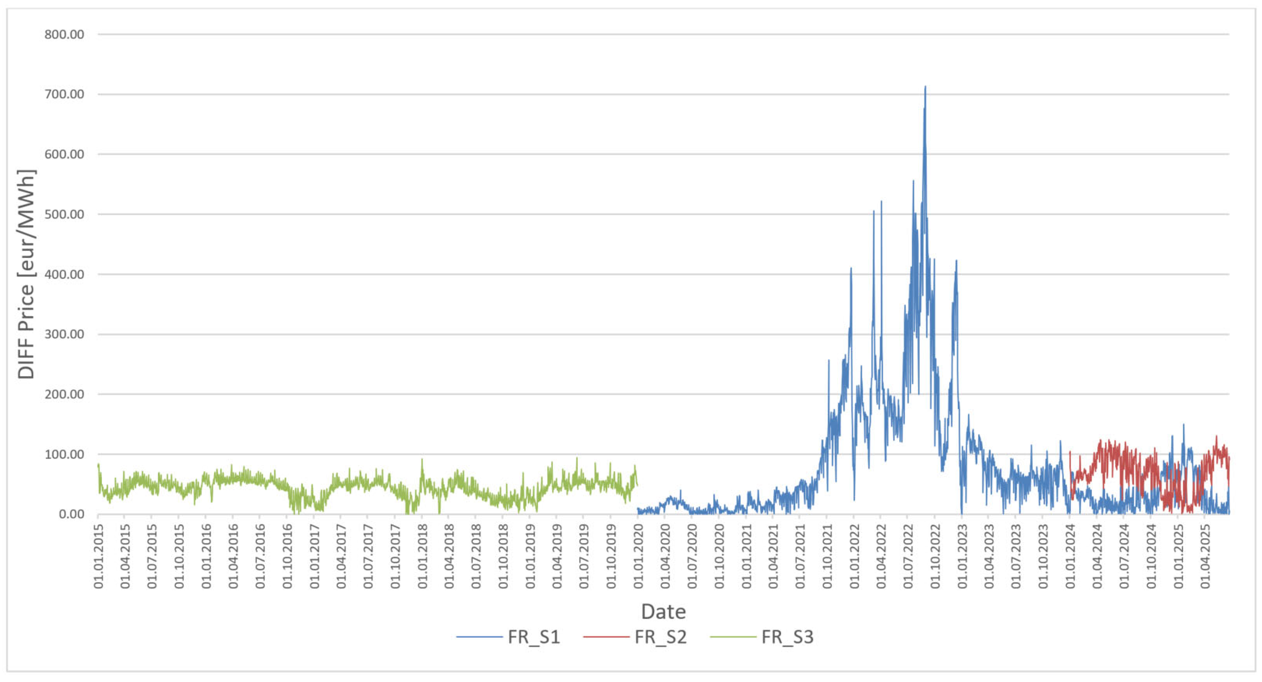
4.2. Research Results of the Static Regression Model for France—Figure 2

For France, the following regression equations were obtained:

Scenario 1: Training data 2015–2019 → forecast 2020–2025

Equation: y = −1.5091 ∗ x + 51.5166

Scenario 2: Training data 2020–2023 → prediction 2024–2025

Equation: y = −1.2540 ∗ x + 143.3906

Scenario 3: Training data 2020–2025 → backcast 2015–2019

Equation: y = −3.0431 ∗ x + 147.9546

In France (Figure 2), we observe a similar trend as for Germany. Scenario S1 fails significantly in the energy crisis—prediction errors reach even more than 600 €/MWh (curve FR_S1). The adaptation of a model trained in stable conditions appears to be inappropriate for turbulent periods. Scenario S2 (curve FR_S2) produces the most accurate predictions, with minimal differences between predicted and actual prices and the price path of the model replicates reality. Scenario S3 (curve FR_S3) has a relatively low error in 2015–2019, but slightly overestimates prices, indicating reduced accuracy when the model is applied backwards from a turbulent period to a calm period. Although it has lower values compared to the S1 scenario (especially in 2021–2022), electricity prices were relatively low in 2015–2019, but the prediction model overestimates them, which may have an undesirable effect in practice.

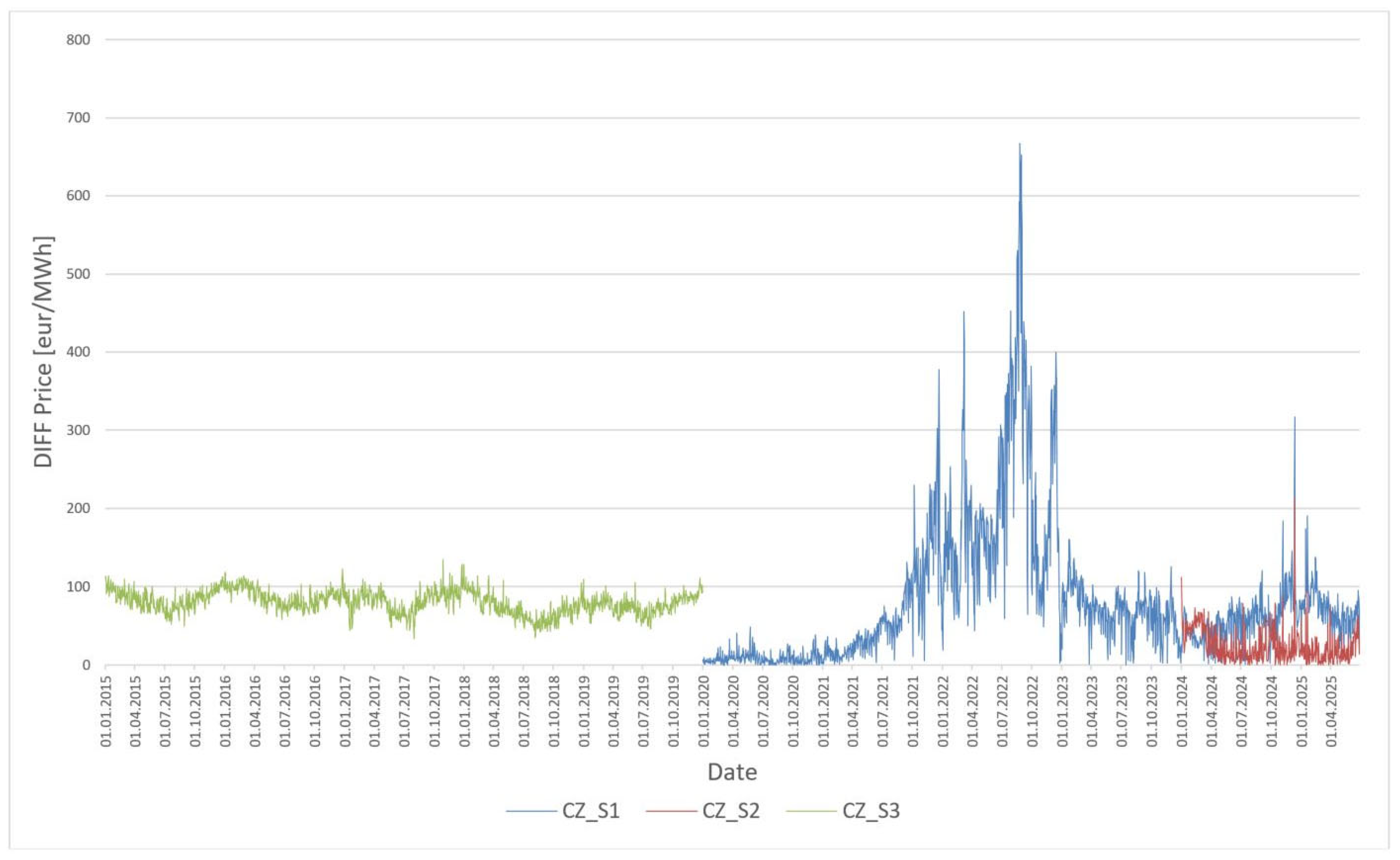
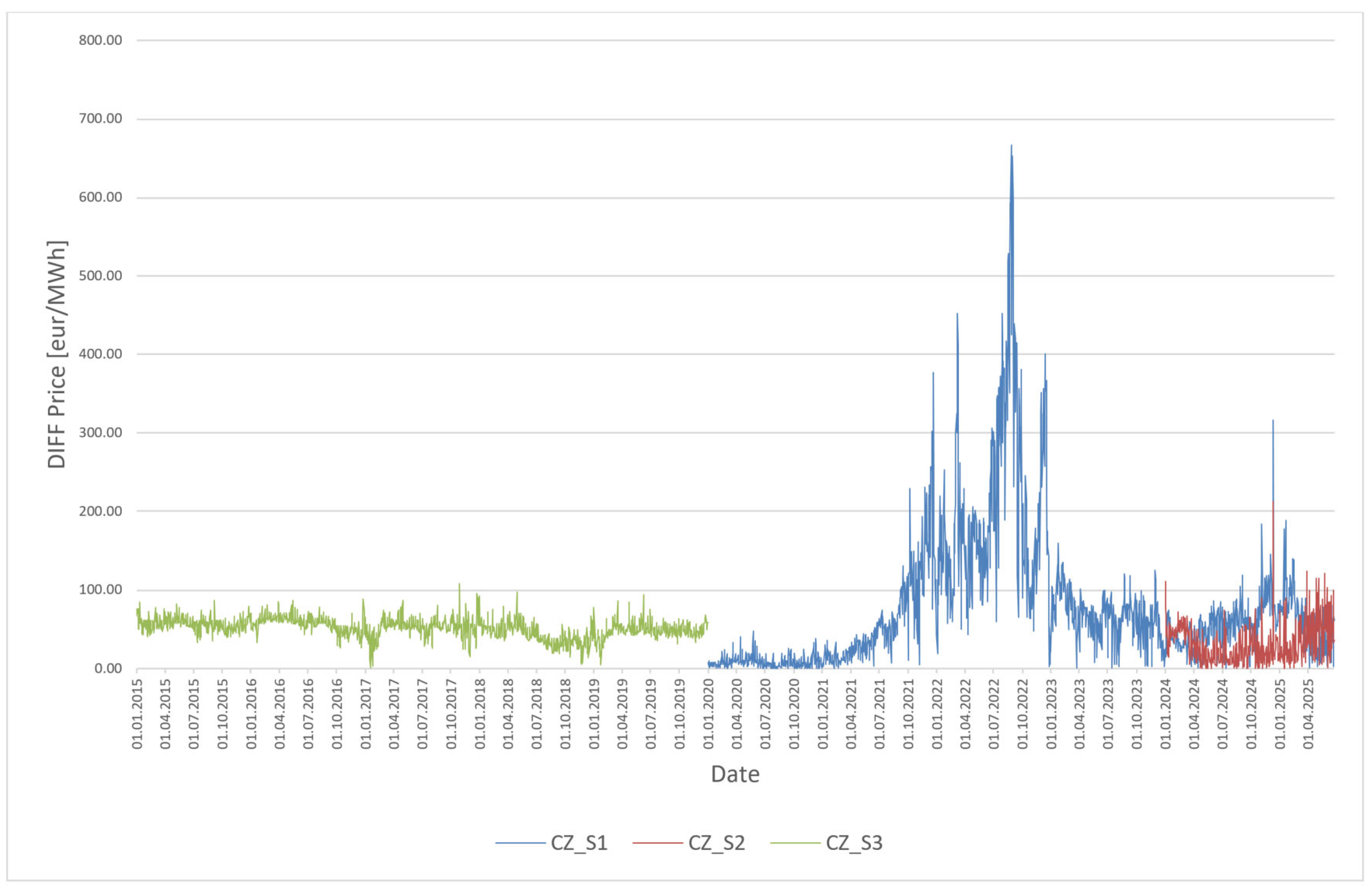
4.3. Research Results of the Static Regression Model for the Czech Republic—Figure 3

The following regression equations were obtained for the Czech Republic:

Scenario 1: Training data 2015–2019→ forecast 2020–2025

Equation: y = −2.0386 ∗ x + 44.5077

Scenario 2: Training data 2020–2023→ prediction 2024–2025

Equation: y = −6.4293 ∗ x + 150.1822

Scenario 3: Training data 2020–2025→ backcast 2015–2019

Equation: y = −6.0296 ∗ x + 140.0907

The results for the Czech Republic (Figure 3) show that scenario S1 (curve CZ_S1) is strongly affected by market volatility after 2020—prediction errors reach extreme values, with the highest in 2022. Scenario S2 (curve CZ_S2), based on data from 2020 to 2023, offers the lowest prediction error rate for the period 2024–2025 and shows a stable path of the difference between predicted and real price. Scenario S3 (curve CZ_S3), which applies the model from the turbulent period to stable conditions, achieves a higher error rate than S2 but lower than S1, confirming that backward application has some limits.

The research results confirm that static regression models are highly sensitive to the choice of the training period. Models calibrated to a stable period before 2020 usually do not achieve satisfactory accuracy in predicting electricity prices in times of increased volatility. In contrast, models built on turbulent data perform better in later years, although their ability to accurately predict prices in more stable environments is limited. This behaviour reflects the changing and non-linear nature of the relationship between the share of renewables and electricity market prices.

The accuracy of the individual static regression models was evaluated using the mean absolute error (MAE) and root mean square error (RMSE) indicators.

Table 3. MAE and RMSE values for scenarios 1, 2, 3 and the countries Germany, France and the Czech Republic—results of the static regression analysis.

Germany
Scenario	S1	S2	S3
MAE	80.24	90.44	105.40
RMSE	120.02	28.80	108.20
France
Scenario	S1	S2	S3
MAE	78.77	66.77	86.64
RMSE	132.46	73.69	88.01
Czech Republic
Scenario	S1	S2	S3
MAE	80.79	25.03	80.20
RMSE	120.95	32.76	81.55

summarises the results obtained for all countries and scenarios analysed. Several key observations can be drawn from these data.

In the case of Germany, the model trained on the stable period 2015–2019 (S1) showed MAE = 80.24 €/MWh, while the model trained on the high-volatility period 2020–2023 (S2) had MAE = 90.44 €/MWh. Despite the assumption of better performance of the models based on turbulent data, their prediction error increased in this case. Model S3, applied in reverse, from a turbulent period to a stable period (2015–2019), achieved the worst accuracy (MAE = 105.40 €/MWh), indicating poor robustness of the transfer of the relationship between variables over time.

In France, the differences between scenarios were less pronounced. Model S1 (stable period) achieved MAE = 78.77 €/MWh, model S2 (volatility) 66.77 €/MWh and back-testing in S3 resulted in an error of MAE = 86.64 €/MWh. This suggests that the French market may be more predictable or less sensitive to the evolution of the share of variable RES in terms of prices.

In the Czech Republic, the results were clearer. Model S2, trained in a period of high volatility, achieved significantly the best accuracy (MAE = 25.03 €/MWh), confirming the suitability of the calibration in challenging conditions. In contrast, model S1 achieved MAE = 80.79 €/MWh, while S3 was at 80.20 €/MWh, indicating the limited predictive power of models based on data from more stable periods.

In summary, the results suggest that the use of static regression models trained on periods of low volatility is not sufficient to accurately predict prices in turbulent environments. However, results from some countries (notably the Czech Republic) show that models trained in challenging environments can be more robust and suitable for future periods with higher levels of uncertainty. This analysis provides a rationale for deploying more flexible, adaptive approaches to forecasting, which are addressed in the next chapter.

5. Research Results of Adaptive Regression Model

This section of the paper presents the results of the application of an adaptive (stepwise) regression model, which was designed to overcome the limitations of classical static models. While the static approach assumes the stability of the relationship between the share of wind and solar generation and the price of electricity throughout the analysis period, the adaptive model allows for a continuous updating of this relationship in response to changing market conditions. A key characteristic of the adaptive approach is the implementation of a sliding window method with a fixed data sample size, which in this research was set to a period of 60 months (scenario S1), 48 months (scenario S2) and 66 months (scenario S3). The aim was not to optimise the length of the sliding window as a hyperparameter, but rather to examine the model’s behaviour under specific market regimes. Scenario S1 represents a period of low volatility prior to 2020. Scenario S2 was designed to reflect the turbulent years 2020–2023, including extreme price fluctuations triggered by geopolitical crises and the rising share of renewable energy sources. Scenario S3 was constructed to evaluate how a model trained on the “new normal” (2020–2025) performs when applied to a preceding stable period (2015–2019). This approach enabled us to compare the forecasting capabilities of the model not only across different methodologies (static vs. adaptive), but also across different market phases and prediction directions.

The adaptive modelling procedure followed the logic of the individual scenarios, which were designed analogously to the static model to ensure comparability of the results of the two approaches. In each scenario, a regression model was initially built based on the same training dataset as for the static model. The resulting equation has the form (2), where, PRICE_(t) is the price of electricity at time t, P_solar+wind is the share of generation from wind and solar together in the total generation at time t (in %), and α, β are the regression coefficients from the sample data.

On the basis of the built model, the electricity price prediction for the first month following the training period was first performed. After this prediction, the model was updated by removing the oldest month from the original training set and replacing it with the latest available month, thus keeping the size of the data window constant. This process was repeated for each subsequent month of the analysis period, with a new regression equation being constructed at each step based on the updated data sample and a price prediction made for the following month. The adaptive model designed in this way ensures that the relationship between the RES share and the electricity price level is continuously updated, thus reflecting current market developments, including changes in the share of renewables, price volatility or externalities. The results of this approach will then be compared with the static model on the same datasets and periods, with an emphasis on evaluating the accuracy of the predictions using MAE and RMSE indicators and on analysing the differences between the two modelling approaches. The adaptive model uses a sliding window method with a constant sample size, which allows for continuous updating of the regression parameters and flexible adaptation of the model to the actual market developments. The results are presented in three separate scenarios for each country, replicating the methodology of the static model and ensuring direct comparability of the outputs:

-

Scenario 1 (S1): Training data 2015–2019, forecast 2020–2025

-

Scenario 2 (S2): Training data 2020–2023, forecast 2024–2025

-

Scenario 3 (S3): Training data 2020–2025, forecast 2015–2019

5.1. Research Results of the Adaptive Regression Model for Germany—Figure 4

In the case of Germany, the graph in Figure 4 shows significant differences in prediction accuracy between the different scenarios of the adaptive model. In the first scenario (S1), where the model was adaptively updated with data from 2015 to 2019 and applied to the turbulent period 2020–2025, the prediction errors gradually increase, especially during the years 2022 and 2023, which were characterised by extreme electricity price volatility. The resulting MAE reached 79.97 €/MWh, confirming the limited ability of the model to adapt to dynamic conditions when the training period does not contain similar fluctuations.

On the contrary, in the second scenario (S2), where the model was continuously updated on data from 2020 to 2023 and then applied to the 2024–2025 forecast, the differences between the predicted and the real electricity price were significantly lower. The MAE and RMSE were only 18.47 €/MWh and 28.80 €/MWh, respectively, the best results among the three scenarios. The graph clearly shows the lowest amplitude of differences in this scenario, which confirms that a model trained in a high-volatility environment is able to predict prices more efficiently under moderately stable conditions.

The third scenario (S3), where the model was trained on the turbulent period 2020–2025 and applied retrospectively to the more stable period 2015–2019, showed deteriorated accuracy. The MAE reached 56.63 €/MWh and the RMSE as high as 108.20 €/MWh. The plot shows more extensive differences compared to the second scenario, indicating that the model trained on highly volatile data is not able to respond flexibly enough when applied to a historically stable period.

5.2. Research Results of the Adaptive Regression Model for France—Figure 5

In the case of France, the graph in Figure 5 confirms the significant differences in predictive performance between the different scenarios of the adaptive model. In the first scenario (S1), in which the model was adaptively trained on data from 2015 to 2019 and applied to the turbulent period 2020–2025, there was a significant deterioration in the prediction accuracy, especially during 2022 and 2023. The resulting MAE reached 81.33 €/MWh, indicating the limited ability of the model trained in a stable environment to react to extreme market fluctuations.

In the second scenario (S2), where the model was trained on data from 2020 to 2023 and then applied to the period 2024–2025, a significant improvement in prediction accuracy was achieved. The MAE dropped to 66.67 €/MWh, which represents a significant reduction in error compared to S1. Nevertheless, the prediction error remains slightly higher than for Germany, indicating the specificities of the French market.

In the third scenario (S3), in which the model was trained on the turbulent period 2020–2025 and applied back to the more stable years 2015–2019, the lowest prediction error was achieved (MAE = 43.38 €/MWh). The graph shows the smallest fluctuations in this scenario, indicating that the model adapted to more complex market behaviour can also perform better with historical data.

These results show that an adaptive model trained on data with a higher degree of variability can provide higher flexibility and in some cases better prediction accuracy, not only for future but also for historical periods with lower volatility.

5.3. Research Results of the Adaptive Regression Model for the Czech Republic—Figure 6

The curves in Figure 6 for the Czech Republic show the differences between actual and predicted electricity prices in the three scenarios of the application of the adaptive regression model. In the first scenario (S1), where the model was trained for the stable period 2015–2019 and applied to the turbulent period 2020–2025, there are significant deviations between prediction and reality. The MAE in this case reaches 79.63 €/MWh, indicating the low ability of the model from the stable period to respond to market fluctuations after 2020.

The second scenario (S2), in which the model was trained on turbulent data from 2020 to 2023 and applied to predict 2024–2025, showed a significant improvement in prediction accuracy. The MAE in this case dropped to 31.00 €/MWh. This result suggests that the adaptive model, if continuously updated during the volatile period, can maintain its prediction accuracy even when the market environment gradually stabilises.

In the third scenario (S3), where the model was trained for the turbulent period 2020–2025 and applied back to 2015–2019, some limitations were again evident. The MAE increased to 51.43 €/MWh. Although this is not the worst result among the scenarios, it is confirmed that the model trained in a high-volatility environment does not achieve optimal accuracy when applied to historical periods with lower market dynamics.

Overall, the adaptive approach improves prediction accuracy, especially when the model reflects the nature of the period to which it is applied. The results for the Czech Republic suggest that the highest accuracy is achieved by a model continuously updated during a turbulent period, which is consistent with the assumption about the benefits of adaptive modelling in volatile market conditions.

In addition to the quantitative evaluation of the prediction errors (

Table 4. MAE and RMSE values for scenarios 1, 2, 3 and the countries Germany, France and Czech Republic—results of adaptive regression analysis.

Germany
Scenario	S1	S2	S3
MAE	79.97	18.47	56.63
RMSE	120.02	28.80	108.20
France
Scenario	S1	S2	S3
MAE	81.33	66.67	43.38
RMSE	132.50	73.52	46.00
Czech Republic
Scenario	S1	S2	S3
MAE	79.63	31.00	51.43
RMSE	120.38	39.89	52.92

), the adaptive modelling results are complemented by a visualisation of the differences between actual and predicted electricity prices (Figure 4, Figure 5 and Figure 6). These graphs provide a detailed view of the evolution of the prediction error over time and allow us to identify in which periods the model was successful and where its accuracy declined.

In the case of Germany, it is clear that the adaptive model trained on a stable period had significant accuracy problems during years of high volatility. In contrast, a model continuously updated during a turbulent period was better able to respond to changing market conditions. The third scenario, which tested the transfer of the model from a period of high volatility to a previous stable period, showed only limited applicability. Similar results are observed in France and the Czech Republic. In all cases, the model that was continuously updated with the most recent data and whose training period matched the nature of the forecast period proved to be the most reliable. In contrast, models applied outside their context (e.g., from a turbulent period to stable years before 2020) showed higher error rates and lower robustness.

Overall, the results show that the adaptive regression approach can significantly improve forecasting accuracy in situations where market conditions change rapidly and where the model needs to be continuously updated based on recent developments. However, they also highlight the limits of the applicability of these models when applied to a different market regime. This confirms the importance of adaptive modelling approaches for electricity markets with a high share of variable renewables.

6. Comparison of Research Results of Prediction Models Based on Static and Adaptive Regression

The research results show that in most cases the adaptive regression model achieves higher prediction accuracy than the static model. This difference is most pronounced in scenarios 2 and 3, where the adaptive model has demonstrated its ability to respond flexibly to changing market conditions and renewable energy share dynamics. In these cases, the adaptive regression systematically reduced the prediction error compared to the static model, confirming its validity especially in situations where the market is in a transitional or post-turbulent phase.

The performance of the adaptive model is benchmarked against the static regression model across all three scenarios (S1–S3) and countries. The comparison is based on standard forecast accuracy metrics—MAE and RMSE—to ensure consistency. The benchmark allows us to determine the predictive improvement achieved through parameter updating and model flexibility.

On the contrary, in Scenario 1, where the model was trained on historical data from a stable period and applied to predict periods of extremely high volatility (mainly 2021–2022), it was shown that switching from static to adaptive regression did not improve the prediction. This suggests that under such radically different conditions, model adaptation alone is not enough—the underlying statistical relationships between variables change so much that regression models, whether static or adaptive, lose the ability to predict reliably.

It should also be taken into account that the entire 2015–2025 analysis period is characterised by an increasing share of RES, which means that regression models have been “learning” over time from data whose structure has been changing continuously. In 2015, the share of wind and PV resources in total generation was significantly lower than in 2025. These structural changes were logically reflected in the change in the relationship between RES and the price of electricity. Moreover, the energy mixes of the countries analysed differ—while Germany has a high share of RES, France is characterised by a strong representation of nuclear power, which partly dampens volatility, and the Czech Republic has a more conservative generation profile. These differences contribute to the different performance of the models across countries.

Overall, the adaptive regression model provides a more reliable and robust tool for predicting electricity prices in an environment where the RES share and market conditions are constantly changing. Its use is most effective in cases where there is some similarity between the training and forecast periods—as was confirmed in scenario 2. Conversely, applying a model from a low volatility period to a highly volatile environment (Scenario 1) proved inappropriate, regardless of whether the model is static or adaptive. Scenario 3 also achieves interesting results, with training data in a more volatile period (2020 to 2025) and prediction data in a lower volatility period (2015 to 2019). Also in this period, the adaptive regression-based prediction model reduces the prediction error and by up to half. Hence, if prices are less volatile in the future, the adaptive regression model is the appropriate prediction model, and the training data could be in the high and average volatility periods, i.e., 2020 to 2025.

7. Hypothesis Testing

In this chapter, the three research hypotheses formulated in the introductory section of this thesis are synthetically evaluated. The evaluation is based on quantitative indicators of prediction accuracy—in particular the mean absolute error (MAE) and the root mean square error (RMSE), which were obtained from the application of static and adaptive regression models to different time scenarios for the three countries analysed: Germany, France and the Czech Republic. The interpretation of the results also took into account the specificities of the countries’ energy markets and the changing share of renewable energy generation over time.

7.1. Testing Hypothesis H1

Hypothesis H1.

The adaptive regression model achieves a lower prediction error (MAE, RMSE) compared to the static model.

The results confirm that the adaptive regression model shows lower prediction error in most cases compared to the static model. This difference is most pronounced especially in Scenario 2, which represents the prediction in the stabilising period 2024–2025, when using a model trained for the turbulent years 2020–2023. In this case, the adaptive model has shown the ability to continuously adapt to the current market developments, thus minimising the prediction errors.

The contribution of adaptive modelling was also strongly evident in Scenario 3, where the model was trained for a high-volatility period (2020–2025) and back-tested for a more stable period (2015–2019). Although in this case the deterioration in accuracy relative to Scenario 2 was evident, the adaptive model still outperformed the static model, which was unable to capture changing market conditions.

The exception is Scenario 1, where the model was trained for the pre-crisis period (2015–2019) and applied to forecast for the highly volatile period 2020–2025. In this case, there was no significant improvement in accuracy when moving from a static to an adaptive approach. While the adaptive method in this scenario showed some robustness to market fluctuations, it did not provide a clear improvement over the static regression. This result suggests that historical models built on stable data are not suitable for forecasting in periods of market volatility—regardless of the regression technique used.

Hypothesis H1 is partially confirmed. The adaptive regression model demonstrates significantly better predictive accuracy in scenarios S2 and S3, but in scenario S1 the differences are not clear-cut, which limits the general validity of the hypothesis to all market situations.

7.2. Testing Hypothesis H2

Hypothesis H2.

The accuracy of the adaptive regression model will be higher in the high-volatility period (2020–2023) compared to the low volatility period (2015–2019).

The results fully support this hypothesis. In Scenario 2, which represents the prediction in the stabilising period 2024–2025 based on the model trained in the turbulent environment 2020–2023, the adaptive model achieved the lowest MAE and RMSE values in all countries analysed. This result shows the strong responsiveness of the model to changing market conditions when trained on data with high electricity price dynamics and variability.

In contrast, in Scenario 3, where the model was applied back to a stable period before 2020, the prediction accuracy decreased, confirming the limited transferability of an adaptive model trained on turbulent data to low volatility conditions. This difference in accuracy clearly supports the conclusion that the adaptive method is most effective in periods where market conditions are dynamically changing.

Hypothesis H2 is fully confirmed. The adaptive regression model has shown higher accuracy in periods of high volatility, and its efficiency is closely related to the timeliness and nature of the input data.

7.3. Testing Hypothesis H3

Hypothesis H3.

Regression models trained in periods of high volatility exhibit lower predictive accuracy when applied to stable market conditions.

This hypothesis focuses on testing the ability of a model trained in a turbulent period (2020–2025) to predict price movements in a more stable market environment before 2020. Testing was conducted under the third scenario (S3) for all three countries, where the adaptive regression model was trained on data from a highly volatile period and then applied to historical data from 2015–2019.

The results show that in all three countries there is a significant deterioration in prediction accuracy under this scenario. The MAE reached 56.63 €/MWh in Germany, 43.38 €/MWh in France and 51.43 €/MWh in the Czech Republic, which are significantly higher values than when applying the same model to the period corresponding to its training base (e.g., in Scenario 2).

The graphical outputs (Figure 4, Figure 5 and Figure 6) also visually confirm that the adaptive models trained in periods of high volatility generated higher deviations when applied to prediction in a more stable period. This phenomenon points to the limited transferability of the model between different market regimes—that is, between environments with frequent price fluctuations and environments dominated by stable, less volatile trends.

These findings are consistent with the assumption that models trained in extreme environments may be “recalibrated” for volatility, reducing their ability to capture the more subtle and stable patterns of price movements typical of periods of lower volatility.

Hypothesis H3 is fully confirmed. The results clearly show that applying a regression model trained during periods of market volatility to stable market conditions leads to a loss of predictive accuracy. This has important implications for the practical application of models in electricity price forecasting, where it is important to consider not only the actual conditions but also the compatibility between the training and prediction periods.

7.4. Testing Hypothesis H4

Hypothesis H4.

Adaptive regression significantly reduces prediction error even when the model is trained on stable market conditions and applied to periods of high volatility.

Hypothesis H4 aims to test whether continuous adaptation of the model can reduce prediction error even when the original training period does not match the nature of the target period. In other words, whether adaptive regression can “correct” the selection of an inappropriate training interval by gradually adapting to new data. In the research, the models in scenario S1 were trained exclusively on historical data from 2015 to 2019, a stable period with low volatility. These models were then used to forecast electricity prices for the turbulent years 2020–2025. Comparison of the results showed a significant difference between the static and adaptive approaches:

-

In Germany, the static model achieved a MAE of 80.24 €/MWh, while the adaptive model reached 79.97 €/MWh.

-

In France, the MAE for the static model was 78.77 €/MWh, while the adaptive model achieved a slightly worse result of 81.33 €/MWh.

-

In the Czech Republic, the adaptive model (MAE = 79.63 €/MWh) improved only slightly compared to the static model (MAE = 80.79 €/MWh).

These results suggest that the adaptive approach cannot significantly reduce the prediction error if the model is based on a historical period that does not fundamentally match the dynamics of the target period. Although there is a slight improvement in the case of Germany and the Czech Republic, the differences are minimal and may be statistically insignificant. In France, even the adaptive regression did not perform better than the static one. Hypothesis H4 was not confirmed. The results show that despite the adaptive model’s ability to respond to new data, the initial choice of training period plays a key role. The high volatility of the target period requires that the training base also contains similar market characteristics. Otherwise, even continuous updating of the model may not lead to a significant reduction in prediction error.

7.5. Testing Hypothesis H5

Hypothesis H5.

Regression models trained in stable periods exhibit lower predictive accuracy when applied to periods of high volatility.

This hypothesis relies on the assumption that models trained on historical data with low price dynamics and stable market conditions (e.g., 2015–2019) do not contain sufficient information to reliably capture the extremes typical of periods of high volatility (e.g., 2021–2022). It is during these turbulent periods that rapid price changes, a significant increase in the share of renewables, as well as increased price sensitivity to external factors, including geopolitical events, occur. Research results support this hypothesis. This hypothesis assumes that a model trained when electricity market prices were highly volatile (e.g., 2020–2025) would not be reliable when applied to forecasting in more stable conditions, such as those typical of the 2015–2019 period. This assumption has been verified in particular under scenario 3 in all three countries analysed. The research results show that in Scenario 3, where the model was trained on turbulent data (2020–2025) and applied back to a stable period (2015–2019), the prediction accuracy was weaker in most cases. Specifically, in Germany, the model achieved MAE = 105.40 €/MWh in Scenario 3, the highest error of all three scenarios. In France, the model from scenario 3 achieved MAE = 86.64 €/MWh, again a worse result than when using the model trained for the steady state period (S1: MAE = 78.77 €/MWh). In the Czech Republic, the error in scenario 3 was very similar to scenario 1 (MAE = 80.20 €/MWh vs. 80.79 €/MWh), indicating a slight loss of accuracy, although not dramatic. These findings confirm that models trained during highly volatile periods have a limited ability to transfer their insights to a stable market environment. This may be due to the asymmetry between market behaviour in times of extremes and in times of normality—other factors come into play during high volatility (e.g., extreme fuel prices, crisis regulatory decisions) that are not present during stable years. Based on the results, hypothesis H5 can be confirmed. In scenario 3, there is a weakening of the prediction accuracy in all three countries when applying the model from a turbulent period to a stable period, with the difference being most pronounced in the case of Germany.

Table 5. Table of hypotheses addressed in the research part.

Hypothesis	Test Result	Note
H1: Adaptive accuracy vs. static	Partially confirmed	Especially in scenarios S2 and S3
H2: Higher accuracy in periods of volatility	Confirmed	Lowest MAE and RMSE in scenario S2
H3: Model from turbulent period = lower accuracy in stable conditions	Confirmed	Scenario S3 for all countries confirms higher errors when applied to 2015–2019
H4: Adaptive regression significantly reduces error even with mismatch between training and target period	Unconfirmed	Adaptive model did not produce significant improvement in scenario S1
H5: Model trained on stable period = higher error in volatile conditions	Confirmed	Scenario S1 shows the highest errors in the 2020–2025 forecast

summarizes the results of the research hypotheses.

Hypothesis H1 was partially confirmed. The modelling results showed that the adaptive regression model shows lower prediction error (MAE and RMSE) compared to the static model, especially in scenarios S2 and S3, i.e., in cases where there was higher market volatility or where the model was continuously updated. However, in the S1 scenario, the adaptive regression did not yield a significant improvement over the static model, suggesting that the advantage of the adaptive approach is particularly apparent in more dynamic market conditions.

Hypothesis H2 was confirmed. The adaptive model performed best in Scenario 2, where it was trained on the turbulent period 2020–2023 and applied to forecast 2024–2025. In all three countries analysed, this scenario produced the lowest values of prediction error, confirming the adaptive model’s ability to respond flexibly to rapidly changing market conditions.

Hypothesis H3, in the updated version focusing on the application of the models from a period of high volatility to a stable market period, was confirmed. Scenario 3 across all countries clearly showed that the model trained in high-volatility conditions (2020–2025) achieved significantly higher prediction error when retrospectively applied to the more stable period of 2015–2019. This result suggests that relationships estimated in extreme market conditions may not be suitably transferable to calmer market phases, confirming the limited generalizability of regression models trained on specific extreme regimes.

Hypothesis H4 aims to test whether adaptive regression can reduce prediction error even when there is a significant mismatch between the nature of the training and target periods—specifically, when the model has been trained in stable market conditions and applied to periods of high volatility. The hypothesis was unconfirmed. The results of the S1 scenario in all three countries analysed showed that the adaptive regression did not yield a substantial improvement over the static approach in this case. Although continuous updating of the model on a monthly basis reduced the prediction error compared to the static model slightly in some cases, in general the prediction error remained high. This suggests that the model’s adaptivity alone is not sufficient to overcome the problems caused by inappropriate choice of training period. These findings confirm that the benefits of adaptive modelling are particularly evident when the training data are representative of the predicted period. The adaptive approach alone cannot compensate for structural differences in market conditions, which reduces its effectiveness when extrapolated to different market regimes. Hypothesis H4 thus highlights the limitations of adaptive regression and also underscores the importance of careful selection of training data in predictive modelling.

Hypothesis H5 was confirmed. The aim of this hypothesis was to test whether models trained on a historically stable period (2015–2019) lose predictive accuracy when applied to periods of high volatility (2020–2025). The research results showed that in all three countries, scenario S1—i.e., a model trained on a stable period and applied to turbulent years—achieved one of the highest prediction errors across all configurations tested. In the case of Germany and the Czech Republic, the S1 scenario in both static and adaptive regression ranked among the least accurate models in predicting 2020–2025. In France, the differences between the scenarios were more moderate, but the trend of worsened performance for the quiet-period training remained. These findings suggest that models trained in low volatility environments fail to reliably capture price dynamics in times of market shocks, reducing their usefulness in predicting future fluctuations. Hypothesis H5 was thus confirmed on the basis of consistent empirical evidence.

8. Conclusions and Discussion

The research results show that the nature of electricity markets has changed fundamentally in recent years—particularly as a result of the sharp increase in the share of variable renewables, geopolitical shocks and changing electricity demand. Traditional static regression models, which assume that the relationships between variables are stable over the entire period of analysis, face a number of limitations in such an environment. This is why an adaptive approach was tested in this paper, which allows models to continuously respond to changing conditions by updating regression parameters.

The empirical results confirmed that the adaptive regression model achieved lower prediction error (MAE, RMSE) in the vast majority of cases compared to the static model (H1), with the largest difference observed in scenarios 2 and 3, which represented prediction during or after turbulent market periods (H2). These findings confirm that the adaptive strategy provides better robustness in modelling prices in high-volatility environments.

Important findings also emerged from hypotheses H3 and H4. It was shown that models trained in high-volatility periods lose predictive accuracy when applied to more stable periods (H3), while models trained in stable environments exhibit the highest errors when applied to the turbulent 2020–2025 period (H4). These results highlight that the performance of regression models is strongly influenced by the relationship between the training and prediction periods—and that extrapolation between fundamentally different market regimes leads to a reduction in model accuracy, regardless of the method used.

Conversely, hypothesis H5, which predicted that adaptive regression would significantly reduce prediction error even with an inappropriately chosen training period (stable data→ volatile period), was not supported. The results showed that even adaptive models are sensitive to consistency between training and target conditions—and adaptivity alone is no guarantee of improvement if the data structure does not match the predicted environment.

At the same time, the regression structure itself (with the share of RES as an explanatory variable) has been shown to be sensitive to both temporal and spatial dimensions. The share of RES varied significantly from year to year—which has a direct impact on the statistical structure of the model. For example, Germany had a higher share of solar and wind than France or the Czech Republic in the period under consideration, which was also reflected in different prediction performances. These differences highlight the need for localised, dynamic models calibrated specifically for particular markets.

Based on the research results, several specific directions for further research can be recommended:

-

Optimising the training window: The use of the length of the training period was a trade-off between robustness and timeliness in this research. Future studies should systematically compare different training window lengths (e.g., 12, 18, 36 months).

-

Change in update frequency: The model was updated every month. Testing quarterly or seasonal updates (e.g., spring–summer–fall–winter) could help better capture seasonal patterns of production and consumption.

-

Accounting for seasonality: Separate models for different seasons could increase the prediction accuracy, especially for variables with a strong seasonal component such as solar radiation.

-

Expansion of the variables entering the prediction model: So far, the model has only used the RES contribution. Expansion to include variables such as consumption, gas prices, CO₂ allowances, imports/exports and meteorological factors could increase the explanatory power of the model.

-

Examination of non-linear models: Adaptive regression is a linear method. In environments with complex market interactions, it is appropriate to test non-linear models (e.g., recurrent neural networks, GARCH models, or hybrid machine learning models).

-

Potential for optimising the length of the sliding training window: Although the primary aim of this research was not to optimise the length of the sliding training window as a hyperparameter, future work could systematically examine how different window sizes affect forecasting accuracy. In this study, the training window length was intentionally tailored to reflect three distinct market regimes: (i) a stable period of low volatility (2015–2019), (ii) a turbulent phase marked by geopolitical shocks and the rising share of renewables (2020–2023), and (iii) the so-called “new normal” (2020–2025). This design enabled the comparison of model performance not only across methodological approaches (static vs. adaptive) but also across different market phases and forecasting directions. However, the question remains whether alternative window lengths—such as 36, 48, or 72 months—could further enhance the model’s adaptability and robustness. Future research could include sensitivity analyses evaluating how different training window lengths influence prediction error, particularly in relation to market seasonality, structural shifts, or long-memory effects in time series data. Promising directions also include dynamically adjustable windows or seasonally weighted updates—such as quarterly shifts reflecting spring–summer–autumn–winter cycles—which could increase modelling flexibility in the rapidly evolving electricity market environment.

-

While the static regression model served as a benchmark for evaluating adaptivity, future research could further enhance the benchmarking process by including non-linear models such as ARIMA, GARCH, or machine learning methods like random forests or neural networks. This would help contextualise the results within a broader modelling spectrum.

Adaptive regression has demonstrated its potential as an effective tool for electricity price prediction in turbulent market conditions. At the same time, however, its effectiveness has been shown to have limitations—especially in cases where the representativeness of the training data is not ensured. The results thus support the need to combine the adaptive approach with better choice of training window, richer data inputs and more advanced analytical techniques. Given the dynamics of energy markets, the development of flexible, robust and adaptive modelling tools is crucial for successful electricity price forecasting in the future. Although the seasonality of renewable energy generation was recognised in the introductory part of the study, it was not directly accounted for in the structure of the regression model. The forecasting model operated on aggregated daily values of RES share, without applying explicit seasonal adjustments or decomposition. This represents a significant limitation, particularly considering the cyclical nature of solar and wind power production. Future research should therefore consider integrating seasonality directly into the model—either by introducing seasonal variables (e.g., quarter, month, or season) or by constructing separate models for different seasonal phases. This approach could substantially enhance the forecasting accuracy, especially in countries with pronounced seasonal fluctuations in RES output.