Degradation-Aware Bi-Level Optimization of Second-Life Battery Energy Storage System Considering Demand Charge Reduction ^†

Abstract

Many electric vehicle (EV) batteries will retire in the next 5–10 years around the globe. These batteries are retired when no longer suitable for energy-intensive EV operations despite having 70–80% capacity left. The second-life use of these battery packs has the potential to address the increasing demand for battery energy storage systems (BESSs) for the electric grid, which will also create a robust circular economy for EV batteries. This article proposes a two-layered energy management algorithm (monthly layer and daily layer) for demand charge reduction for an industrial consumer using photovoltaic (PV) panels and BESSs made of retired EV batteries. In the proposed algorithm, the monthly layer (ML) calculates the optimal dispatch for the whole month and feeds the output to the daily layer (DL), which optimizes the BESS dispatch, BESSs’ degradation, and energy imported/exported from/to the grid. The effectiveness of the proposed algorithm is tested as a case study of an industrial load using a real-world demand charge and Real-Time Pricing (RTP) tariff. Compared with energy management with no consideration of degradation or demand charge reduction, this algorithm results in 71% less degradation of BESS and 57.3% demand charge reduction for the industrial consumer.

1. Introduction

To curb CO₂ emissions and combat climate change, electric vehicles (EVs) are replacing conventional vehicles. In 2024, the total number of EVs reached 40 million worldwide [1]. The degradation of EV battery packs leads to their retirement as they are no longer suitable for the vehicle energy demands due to their power limitation. EVs have been on the road for over a decade. That means that the combined capacity of retired battery packs will reach 200 GWh by 2030 [2]. These retired battery packs still have 70–80% capacity left [2]. On the other hand, the demand for BESSs is expected to cross 183 GWh by the year 2030 [3]. If second-life batteries can be utilized in energy storage systems for the electric grid, they could significantly alleviate the demand for BESS.

Retired batteries can be disposed of as land waste, recycled, or repurposed for second-life use [4]. However, the reuse of retired batteries as second-life BESS for the grid is increasing rapidly. BESS is subjected to less intensive demands in grid applications than electric vehicles, which makes re-purposing SLBs for BESS a suitable choice. Moreover, SLBs create a strong circular economy throughout the battery supply chain and lead to the extraction of the maximum value from EV batteries before recycling [5]. This is exemplified by recent interest from leading automotive companies and recyclers in using retired batteries for the grid  [6].

Thirteen application areas and three stakeholders for the energy storage system in an electric grid are identified in [7]. The three stakeholders are transmission system operators (TSO), utility companies, and consumers [7]. The usage of BESS to meet part of the load to reduce the peak demand is called peak shaving. For commercial electricity customers, this would reduce the demand charge—an extra energy charge co-related to the peak load demand in a specified time frame, calculated in $/kW [8]. The demand charge represents 30–70% of the electricity bills for industrial or commercial consumers [9].

1.1. Literature Study

The first-life use of EV batteries dictates the trajectory of degradation in their second life [10]. The underlying phenomenon for the degradation in SLBs is quite similar to the fresh batteries that include dendrite formation, loss of lithium on the electrodes, solid electrolyte interphase (SEI) layer growth, etc. [4]. However, the rate and percentage of these individual factors affecting the degradation vary. Each cell inside an EV pack is subjected to varying loads. By the time the battery pack is retired from the EVs, the inherently small manufacturing differences result in varying cell capacities. It is therefore difficult to generalize a model for the degradation behavior of SLBs. Unlike fresh batteries, SLBs are prone to knee point—the point in the capacity curve where cells undergo rapid degradation. The active management of SLB packs is important to delay the knee point as much as possible. Moreover, BESS operation for the grid must be a trade-off between BESS’s use and its degradation. As the availability of data from real-world aging cycles for SLBs increases, data-driven models increasingly give an insight into the degradation behavior of SLBs. Many prior works have used mixed-integer linear programming (MILP) to optimize the SLB operation for different use cases: In [11,12,13,14,15], the retired batteries for supporting EV fast charging station loads are evaluated. Microgrid day-ahead scheduling using the retired batteries without considering the degradation behavior was investigated in [16,17]. In [18], the capacity loss of SLBs was modeled using the Arrhenius degradation model extensively used for fresh batteries. In [19], the authors make use of short- and long-term estimation and prediction of BESS’s state of health (SoH) in a dispatch profile to perform energy balancing and energy arbitrage (EA).

Many works have shown that second-life BESS and other co-located distributed energy resources (DERs) can help reduce the demand charges, but they either do not consider BESS degradation or use the simplified degradation models. To our knowledge, this is the first attempt to design a degradation-aware energy-optimized dispatch for a second-life BESS to reduce demand charges of an industrial customer where a degradation model is derived based on real-world aging data for the SLBs. Previously in [20], an optimization framework for SLBs was presented. This work is an extension of that framework by considering the battery degradation in detail.

Table 1. Comparison of key works on second-life battery optimization and applications.

Reference	Focus Area	Approach/Limitation	Contribution
[11]	SLBs for EV fast charging	MILP-based planning for centralized charging with second-life batteries; no degradation modeling	Demonstrates cost-effective charging using SLBs
[12]	Nanogrid fast charging station with SLBs	Uses machine learning for fuzzy EMS, but lacks detailed SoH/degradation handling	Proposes EMS for urban nanogrids with SLB-PV setup
[14]	SLBs in fast charging	Simulation-based performance study; limited degradation modeling	Evaluates SLB viability for high-power charging needs
[16]	Microgrid planning with SLBs	Focuses on carbon reduction feasibility; excludes SLB degradation effects	Assesses shared SLB systems in renewable-powered microgrids
[17]	SLBs as flexible grid loads	Optimizes power dispatch; no online SoH modeling	Demonstrates SLBs as dispatchable DERs
[19]	SoH-aware SLB operation	Uses online SoH estimation for dispatch optimization	Introduces online degradation tracking into optimization

shows the recent works done on SLB optimization and grid applications.

1.2. Contributions

The main contributions of this paper are as follows:

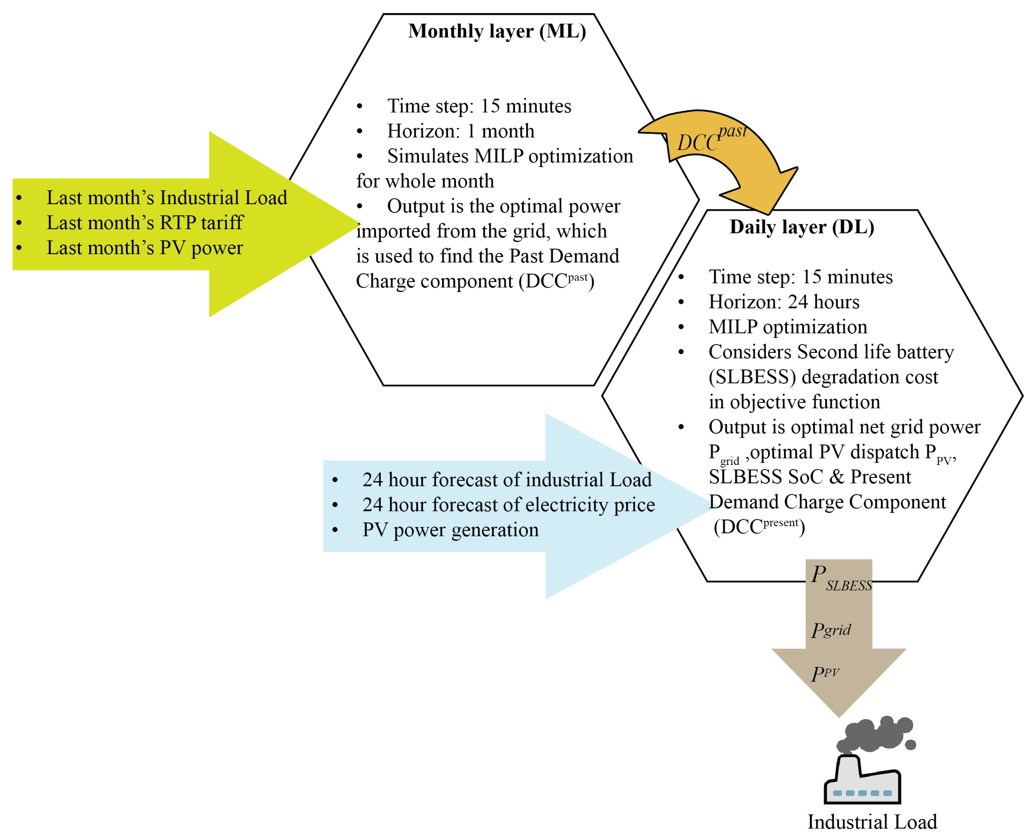
• A bi-level energy management (BL-EM) algorithm is proposed consisting of a monthly layer (ML) and daily layer (DL). The monthly dispatch and the previous month’s demand charge thresholds are calculated in the ML, which is fed into the DL calculating the optimal dispatch of second-life BESS, power imported from the grid, power exported to the grid, and photovoltaic (PV) power.
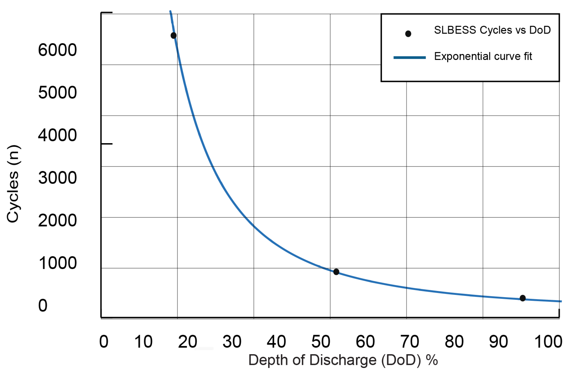
• In contrast with the literature, this article uses the real-world aging cycle data from [21] to generate a Wöhler curve (cycle vs. depth of discharge (DoD)) for a second-life Li-NMC (Lithium Nickel Manganese Cobalt oxides) battery pack. The equation obtained by applying piecewise fitting on the Wöhler curve is used to model the BESS degradation in the DL. Deep cycling and frequent use shorten the life of the BESS, causing it to reach the knee point. From the perspective of SLB, for the first time, an optimized trade-off is presented between BESS utilization and energy arbitrage (EA).

The paper is divided into the following sections: Section 2 presents the BL-EM framework along with detailed second-life BESS degradation and demand charge modeling. Section 3 presents the results of the simulation on a case study, followed by a discussion in Section 4.

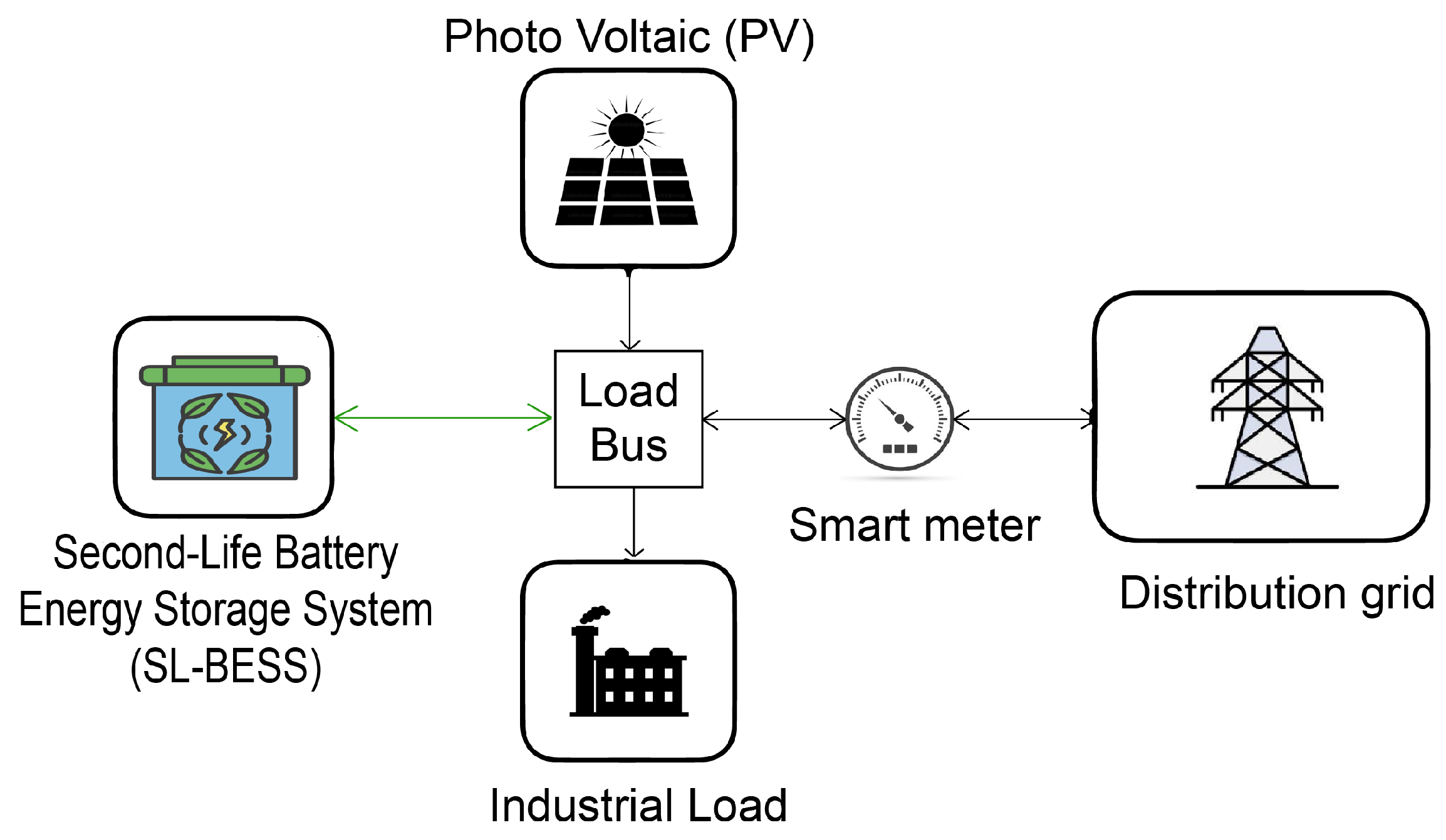
2. Bi-Layer Energy Management Framework

The bi-level energy management framework (BL-EM) is presented in this section and shown in Figure 1. The framework considers an industrial load subjected to demand charges from the electrical utility. BESSs made of retired LMO+NMC batteries along with co-located PV generation, which are used to meet the load demand, are shown in Figure 2. Moreover, a net metering approach capable of feeding the power back to the grid is considered to perform the energy arbitrage. Energy arbitrage is a technique where power is used to charge the BESS when a utility’s cost per kWh is low, and BESS is discharged when the cost per kWh is high. The optimization framework optimizes the dispatch of BESS to reduce the demand charge tariff while keeping its degradation in check. This trade-off is important for the longevity of the BESS as it can undergo rapid degradation under extensive use.

2.1. Monthly Layer (ML)

ML is the top layer that optimizes the power generation for the whole month based on the monthly load and PV output forecasts. This layer forwards the value of the historical demand charge component $DC{C}_{historical}$ to the DL at the start of the month. The planning horizon of the ML is 1 month with a time step of 15 min. In this work, a demand charge tariff of 13.33 USD/kW [22] is considered.

2.2. Second-Life Battery Energy Storage System Model

The second-life BESS is different from a fresh BESS in terms of its capacity degradation, cell balancing requirements, and power electronics interface [4]. Depending on the electrical load, the second-life BESS can comprise a single retired EV battery pack or a combination of several battery packs. When combining several packs to form one BESS, packs with fairly identical capacities should to be selected. This can save costs in designing complex active balancing in the battery management system (BMS) that will be required with packs having varied starting capacities [23].

2.2.1. Wöhler Curve Derivation for Second-Life NMC+LMO Battery

The Wöhler curve is used to include the degradation of fresh batteries in the optimization algorithms [24]. This curve represents the number of cycles n versus the depth of discharge for different battery chemistries and is obtained from the original manufacturers of batteries or derived by performing accelerated life testing (ALT) experiments in the laboratory. However, for SLBs, such a curve is missing because the manufacturers only guarantee the use of batteries for the first life (till 80%). Therefore, a Wöhler curve for the fresh battery is not valid for SLB despite having the same characteristics, e.g., chemistry and capacity. Moreover, because the interest in SLBs is newfound, the data for ALT for SLBs are also not easily available. Some researchers [25,26,27,28] have conducted aging cycles on retired battery cells. These datasets are of limited use since the batteries have been subjected to a narrow set of aging conditions and cannot be used to derive a generalized model. It is therefore very difficult to generalize a Wöhler curve for different SLB chemistries or even two different battery packs of the same chemistry. Nissan Leaf Gen 1 battery packs are evaluated by performing ALT in [29]. In this paper, we use a real-world aging dataset from [21] to generate a Wöhler curve for LMO+NMC battery cells. The cell characteristics for the dataset are presented in

Table 2. SLB cell specifications from [21].

Cell number	18,650
Positive electrode material	NMC+LMO
Cell capacity	2.15 Ah (fresh), 1.72Ah (@ 80% capacity)
Nominal Voltage	3.65 V

. NMC+LMO is one of the most used Li-ion battery types in EVs, such as Tesla and Nissan Leaf, and a significant percentage of retired EV batteries will be NMC+LMO. In [21], the authors presented a classic exponential-based capacity loss model for SLB considering three stress factors: depth of discharge ($DoD$), mean state of charge, and C-rate. The capacity loss ($Q_{loss}$) vs. capacity throughput ($Q_c$) of three different cells from the SLB pack using the data from [21] is shown in Figure 3. Full equivalent cycles n can be expressed in terms of $Q_c$ by (1).

$$FEC\left(n\right)={\displaystyle \frac{CapacityThroughput}{DoD·RatedCapacity}}={\displaystyle \frac{Q_c}{DoD·C_{rated}}}$$

(1)

For Cell 1, Cell 2, and Cell 3, n is 274, 971, and 6285, respectively, till reaching the end of life (EoL) when capacity reaches 30%. Plotting the n and $DoD$ data, the Wöhler curve is obtained by fitting an exponential curve, as shown in Figure 4. The coefficients a, b, and c for the exponential curve fitting in (2) are 2731.7, 0.679, and 1.614. This curve is used in the DL to model the degradation of BESS.

$$n=a·Do{D}^{-b}·e^{c(1-DoD)}$$

(2)

2.2.2. Battery Degradation Model

EV batteries go through two types of degradation, calendar degradation and cyclic degradation. Calendar degradation occurs even when the battery is unused. Cyclic degradation, on the other hand, is the degradation caused by the use cycles of the battery when the battery is charged and discharged [30]. The Wöhler curve derived earlier for the second-life BESS is used in the DL for the BESS degradation modeling. In this work, it is assumed that the BESS is placed in a controlled environment where the temperature and other environment variables are maintained, resulting in minimum calendar degradation. Calendar degradation is therefore omitted from the battery degradation calculations. The use of batteries in the grid is relatively less energy intensive as compared with their use in EVs; therefore, it is possible to use BESS at a C-rate of less than 1 C. Works in [31] have shown that maintaining a C-rate of less than 1C slows down the degradation of SLB significantly. In [32], a rare phenomenon of capacity throughput increase for eight retired lithium manganese oxide (LMO)/graphite pouch cells from Nissan Leaf battery packs was observed. This is attributed to cycling at lower C-rates and increased temperature. In this paper, we assume that the BESS operates at a constant rate equal to C/2 until the EoL. The BESS degradation cost $C_{deg}$ in dollars ($) is given by (3), where $CCos{t}_{BESS}$ is the capital cost of the BESS, n is the number of cycles the BESS is capable of undergoing before the EoL, and $C_{rated}$ is the initial capacity of the BESS in kWh.  

$$C_{deg}={\displaystyle \frac{CCos{t}_{BESS}}{n}}·C_{rated}$$

(3)

The capital cost of BESS fluctuates highly and depends on many variables. In [33], the authors formulated an economic framework to predict the USD/kW rate of SLBs until 2050 under various EV uptake scenarios, and the results showed that, in all the scenarios, the cost of SLB plateaus was around 50 USD/kW. Therefore, 50 USD/kWh is chosen as the capital cost for BESS in this article. In addition to capital costs, there are refurbishment, labor, and maintenance costs, which are not considered in this work due to their high dependency on battery type and location. Practically no BESS experiences the same DoD at every cycle of its lifetime; rather, it charges and discharges at varied DoD levels throughout its operation, which makes it difficult to find the fixed n. Therefore, (3) cannot be implemented in this form. To overcome this problem, a rain-flow counting algorithm (RCA) [34] is leveraged from the literature, which defines a new dummy variable. The dummy variable is an intermediate $So{C}_{dummy}$ that takes the SoC value during the discharge operation and the SoC value of a previous step during the charge operation. Given that n is a function of $DoD$, where $DoD=1-SoC$, $C_{deg}$ is also a function of $DoD$ and $SoC$. Mathematically, the dummy variable $So{C}_{dummy}$ and $C_{deg}$ at each time step can be written as

$$So{C}_{dummy}=So{C}_{t-1}-{\displaystyle \frac{E_{discharge}}{{\eta }_{discharge}{C}_{BESS}}}·100$$

(4)

where $E_{discharge}$ is the energy discharged and $C_{BESS}$ is the capacity (kWh) of the BESS.

$$\begin{array}{cc}\hfill C_{deg}=C_{deg}\left(So{C}_{dummy}\right)-& \hfill \\ \hfill C_{deg}\left(So{C}_{t-1}\right)\end{array}$$

(5)

The above equation can be revised to express in terms of the actual $SoC$ variable as

$$\begin{array}{c}\hfill C_{deg}=\left\{\begin{array}{cc}{C}_{deg}\left(So{C}_t\right)-C_{deg}\left(So{C}_{t-1}\right),Discharge\hfill & \\ 0,Charge\hfill \end{array}\right.\end{array}$$

(6)

The above equation is nonconvex, which means that it results in multiple local minima and increased computational complexity in finding the global optimum. It can be transformed to MILP by splitting SoC into $\nu$ segments [35] using a piecewise defined function (7). Consequently, the modified BESS degradation cost $C_{deg}^{\prime }$ can be written as

$$\begin{array}{cc}\hfill C_{deg}^{\prime }\left(t\right)\approx \sum _{\nu =1}^2\sum _{t=1}^{96}({\mathrm{\Lambda }}^s(t,\nu )C_{deg}(SoC+(\nu -1)\mathrm{Y})+& \hfill \\ \hfill \psi \left(\nu \right)SoC(t,\nu )\end{array}$$

(7)

where

$$\begin{array}{c}\hfill \mathrm{Y}=\left({\displaystyle \frac{\overline{SoC}-\underline{SoC}}{\nu }}\right)\end{array}$$

(8)

$$\begin{array}{c}\hfill \psi \left(\nu \right)=(C_{deg}(\underline{SoC}+\nu \mathrm{Y})-C_{deg}(\underline{SoC}+(\nu -1)\mathrm{Y}))\mathrm{Y}\end{array}$$

(9)

$$\begin{array}{c}\hfill \sum _{\nu =1}^2\sum _{t=1}^{96}\mathrm{\Lambda }(t,\nu )=1\end{array}$$

(10)

$$\begin{array}{cc}\hfill \underline{SoC}+\sum _{\nu =1}^2\sum _{t=1}^{96}SoC(t,\nu )+(\nu -1)\mathrm{Y}\mathrm{\Lambda }(t,\nu )& =\hfill \\ \hfill SoC(E_{charge}\left(t\right),E_{discharge}\left(t\right)\end{array}$$

(11)

$$\begin{array}{c}\hfill 0\le So{C}_t^{\nu }\le \mathrm{Y}{\mathrm{\Lambda }}_{\nu }t\end{array}$$

(12)

Equations (10)–(12) represent the constraints for a piecewise formulation (7). One segment of the piecewise formulation must be selected at each t, which is made sure by constraint (10). The piecewise calculations are linked to the BESS actual $SoC$ and dummy $So{C}_{dummy}$ (4) by (11). The lower and the upper bounds for the SoC segment length are given by (12). Note that SoC in (8)–(12) takes the values of both the actual $SoC$ and $So{C}_{dummy}$ separately while calculating $C_{deg}^{\prime }$ in (7).

2.3. Demand Charge Reduction Modeling

Demand charge makes up approximately 30–70% of an industrial consumer’s bill [9]. It is the part of the electricity tariff that is added on top of the energy consumption charges and is calculated based on the 15 min peak power demand (kW) in a particular month. One way to reduce the demand charge part of the electricity bill is to shift the consumer’s peak load to less load-intensive hours. However, this is not possible in the case of large industrial loads. A practical solution is to use distributed energy resources (DERs) like PV, wind, or BESS to meet the peak load. The $DC{C}_{past}$ obtained from the ML is fed to the DL that optimizes the net power imported from the grid and battery charge/discharge power, keeping the demand charge at a minimum. The DL updates its $DC{C}_{present}$ by selecting the maximum of the power imported from the grid $E_{grid}^{+}/\mathrm{\Delta }\left(t\right)$ and historical demand charge from $DC{C}_{past}$ once per day, as given in (13).

$$DC{C}_{present}=max({\displaystyle \frac{E_{grid}^{+}}{\mathrm{\Delta }t}},DC{C}_{past})$$

(13)

Because the optimization problem in the DL is formulated as a minimization (14), the algorithm will try to minimize net grid imports and, hence, the demand charge. An amortized variable ${\pi }_{amortized}={\displaystyle \frac{\pi }{(\gamma -d)+1}}$ is introduced in the cost function, where $\pi$ is the demand charge tariff ($/\mathrm{kW}$) of the utility, $\gamma$ is the billing period that equals 31 days a month, and d is the scheduling horizon that continues to iterate with every passing day of the month, increasing as the number of days in the month passes. ${\pi }_{amortized}$ optimizes ($DC{C}_{present}$). However, the monthly demand charge is decided based on the trade-off with the battery degradation cost.

2.4. Daily Layer (DL)

The DL has a shorter planning horizon of 24 h with a time step of 15 min. The DL optimizes a mixed-integer linear programming (MILP)-based cost function for all the days of a particular month based on the day-ahead load and PV forecast. The historical $DC{C}^{past}$ coming from the ML is used in the objective function to decide the maximum 15 min power imported from the grid. The decision variables for UL are $[E_{grid}^{+}\left(t\right),E_{grid}^{-}\left(t\right),C_{degradation}\left(t\right),DC{C}_{present}]$. All decision variables are computed every 15 min for a total of 96 times per day except $DC{C}^{present}$.

2.4.1. Cost Function

The cost function of the DL in (14) is a trade-off between the cost of energy imported/exported to/from the grid, SLBESS degradation cost, and demand charge component $\left(DCC\right)$.

$CostFunctio{n}_{DL}=$

$$\begin{array}{cc}\hfill min\sum _{d=1}^D\left(\right(\sum _{t=1}^{d+96}\stackrel{Energyimport/exportfromthegrid}{\overbrace{(E_{grid}^{+}\left(t\right)x_{sell}\left(t\right)-E_{grid}^{-}\left(t\right)x_{buy}\left(t\right))}}+& \stackrel{second-lifeBESSdegradationcost}{\overbrace{\left(C_{deg}^{\prime }\left(t\right)\right)}})\hfill \\ \hfill +\stackrel{Demandchargecomponent}{\overbrace{\left(DC{C}_{present}\left(d\right){\pi }_{amortized}\right)}})\end{array}$$

(14)

The decision variables are energy imported from the grid $E_{grid}^{+}\left(t\right)$, energy exported to the grid $E_{grid}^{-}\left(t\right)$, degradation cost of BESS $C_{deg}^{\prime }\left(t\right)$, and current demand charge component $DC{C}_{present}\left(d\right)$.The cost function is calculated 96 times per day for every 15 min interval and repeated for each of the 31 days of the month.

2.4.2. Constraints

$$\begin{array}{cc}\hfill E_{grid}^{+}\left(t\right){\eta }_{(P.E)}+P_{pv}\left(t\right)+E_{discharge}\left(t\right)=& \hfill \\ \hfill Load\left(t\right)+E_{charge}\left(t\right))+{\displaystyle \frac{E_{grid}^{-}}{{\eta }_{(P.E)}}}\forall t\end{array}$$

(15)

$$\begin{array}{c}\hfill E_{grid}^{+}\left(t\right)\ge 0,E_{grid}^{-}\left(t\right)\ge 0\forall t\end{array}$$

(16)

$$E_{grid}^{+}\left(t\right),E_{grid}^{-}\left(t\right)>=M(1-u_1\left(t\right))\forall t$$

(17)

$$E_{charge}^{+}\left(t\right),E_{discharge}^{-}\left(t\right)>=M(1-u_2\left(t\right))\forall t$$

(18)

$$0\le E_{charge}\left(t\right)\le P_{BESS}^{rated}\mathrm{\Delta }t\forall t$$

(19)

$$0\le E_{discharge}\left(t\right)\le P_{BESS}^{rated}\mathrm{\Delta }t:\forall t$$

(20)

$$\begin{array}{cc}\hfill SoC\left(t\right)=SoC(t-1)+{\eta }_{charge}{\displaystyle \frac{E_{charge\left(t\right)}}{C_{BESS}}}100-& \hfill \\ \hfill {\displaystyle \frac{E_{discharge}\left(t\right)}{{\eta }_{discharge}{C}_{BESS}}}100\forall t\end{array}$$

(21)

$$E_{charge}\left(t\right)\le {\displaystyle \frac{\overline{SoC}-So{C}_{t-1}}{100}}.C_{BESS}\forall t$$

(22)

$$E_{discharge}\left(t\right)\le {\displaystyle \frac{So{C}_{t-1}-\underline{SoC}}{100}}{C}_{BESS}\forall t$$

(23)

$$\begin{array}{c}\hfill -RR·\mathrm{\Delta }t\ge E_{grid}^{+}\left(t\right)\le RR·\mathrm{\Delta }t\forall t\end{array}$$

(24)

$$P{V}_{pu}\left(t\right)=0.92Irr\left(t\right){\displaystyle \frac{(1-\rho \mathrm{\Delta }t)}{1000}}\forall t$$

(25)

The constraint (15) makes sure that generation meets the load at each time step $\mathrm{\Delta }$t. The constraint (16) means that the energy imported/exported from/to the grid is either 0 or positive. Introducing the binary variables $u_1\left(t\right)$ and $u_2\left(t\right)$ in the objective function will make it non-linear. Therefore, the big-M method is used in (17) and (18). These two constraints ensure that the battery either charges or discharges and that the energy is either imported or exported from the grid at each $\mathrm{\Delta }$t. The upper and lower limit of BESS charge and discharge energy are set in (19), where $P_{BESS}^{rated}$ is the BESS rated power (kW). The state of charge $\left(SoC\right)$ at each time step is calculated by (21) according to the BESS charge ${\eta }_{charge}$ and discharge ${\eta }_{discharge}$ efficiencies. To ensure that the charge and discharge energy values of the BESS are within the available energy limits constraint, (21) is used. The grid ramp rate $\left(RR\right)$ in (24) is taken as 100 kW/s, which is the maximum amount of power that the distribution grid can provide or absorb. This constraint keeps the grid energy limit within the ramp rate limit. $\overline{SoC}$ and $\underline{SoC}$ are the upper and lower state of charge limits, used as 90% and 30% in this work. The PV panel output is subjected to the constraints of available power in (25), which is a function of irradiance ($Irr$) at each time step t. Algorithm 1 shows the complete bi-layer energy management algorithm.

Algorithm 1 BL-EM Algorithm

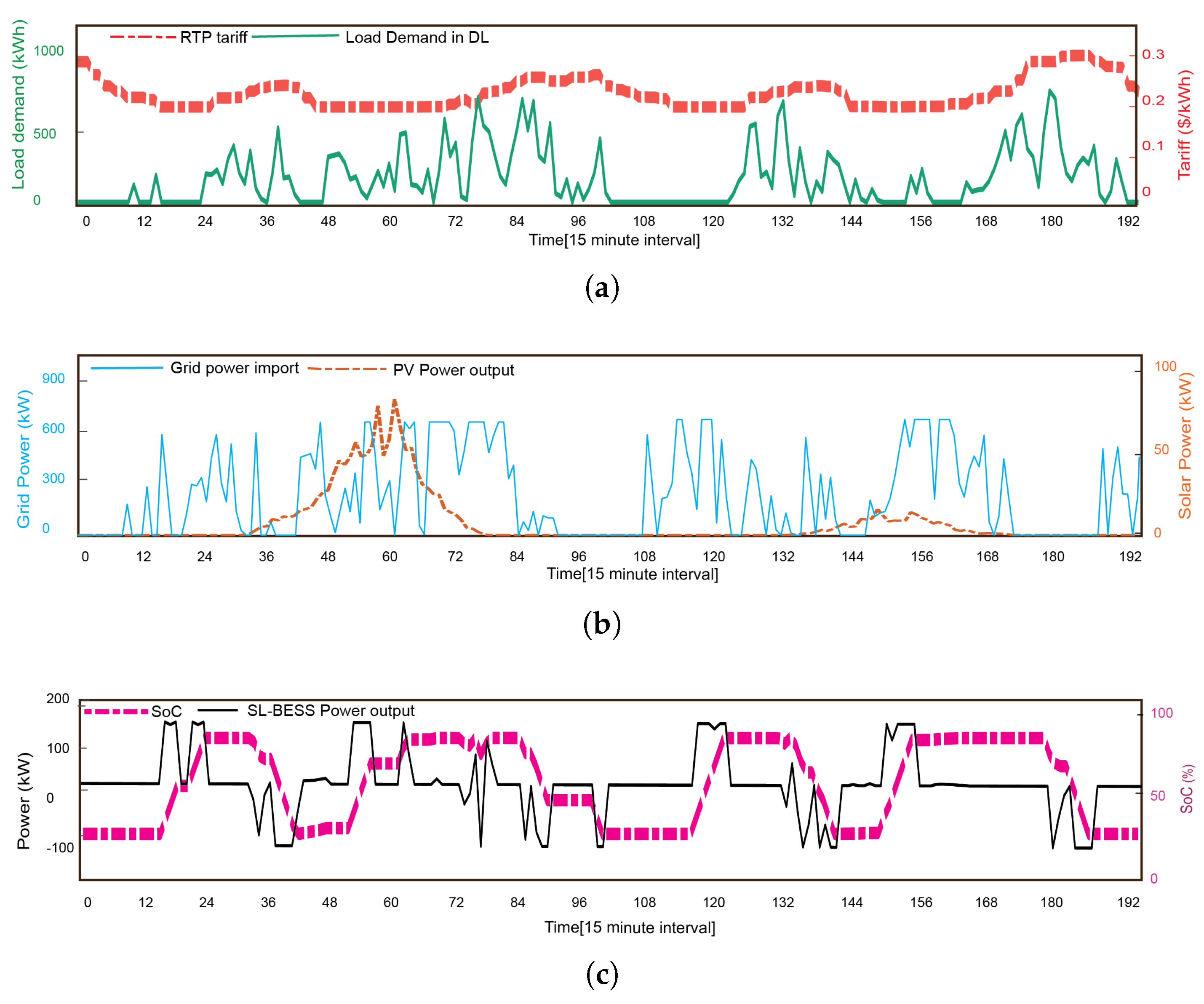
1: Import load, energy tariff, and PV output data from the previous month. 2: Optimize the peak power import in ML to obtain $P_{\max }^{\mathrm{ML}}$. 3: Set $DC{C}^{\mathrm{past}}=0.8\times P_{\max }^{\mathrm{ML}}$. 4: Feed $DC{C}^{\mathrm{past}}$ into the DL model. 5: for $d=1$ to D do 6:     for $t=1+96(d-1)$ to $96+96(d-1)$ do 7:         Import forecast data $[\mathrm{Load}\left(t\right),P_{\mathrm{PV}}\left(t\right),\mathrm{\Lambda }\left(t\right)]$ for a horizon of T. 8:         Minimize the cost function (14) over the decision vector $\{DC{C}^{\mathrm{past}},E_{\mathrm{grid}}^{+}\left(t\right),E_{\mathrm{grid}}^{-}\left(t\right),C_{\mathrm{degradation}}\left(t\right),DC{C}_{\mathrm{present}}\}$, subject to constraints (4)–(12) and (15)–(25).

3. Results

In this section, the bi-layered energy management algorithm (the optimization algorithm is run on an Intel(R) Core(TM) i5-8350U CPU @ 1.90 GHz, with 16 GB RAM; the simulation took 8 min and 7 s) is tested for a medium-sized industrial consumer. The details of the parameters used for the case study are listed in

Table 3. Parameters used for the case study.

Parameter	Value
PV panel rating [kW]	100 kW
BESS rating [kWh]	360 kWh
BESS no. of battery packs	12
Battery chemistry	Li-ion (NMC+LMO)
BESS pack ratings	30 kWh capacity 24 modules 8 cells/module
BESS capital cost [$/kWh]	$50/kWh
AC/DC, DC/AC converter efficiency ${\eta }_{\mathrm{PE}}$	98%
BESS charge efficiency ${\eta }_{\mathrm{charge}}$	98%
BESS discharge efficiency ${\eta }_{\mathrm{discharge}}$	98%
Demand charge tariff $\gamma$ [$/kW]	13.33

. The BESS capacity is 360 kWh and is made up of 12 packs of retired Nissan Leaf generation 2 batteries with an original capacity of 40 kWh each. Each battery pack considered has 75% of the nominal capacity, i.e., 30 kWh (30 × 12 = 360 kWh). The PV panel has an installed capacity of 100 kWh. The demand charge tariff considered is from the DTE utility of Michigan’s D11 Primary Supply tariff [22] for industrial consumers that range from 3.56 USD/kW for the capacity load to 13.33 USD/kW for a non-capacity load. The Real-Time Pricing (RTP) tariff is taken from an online source from the Singapore electricity market. The industrial load profile is obtained from a public dataset. Please note that the algorithm can take varied amounts of time, depending on the load profile, tariff data, and other input parameters.

In Figure 5, the results are plotted for 2 days divided into 15 min periods. Figure 5a shows the RTP tariff (USD/kWh) and actual load demand (kWh). Figure 5b shows the solar PV output and the grid’s imported energy. Figure 5c shows the optimal dispatch of BESS in the DL. The BESS charge and discharge are optimized such that they charge only at the time of low RTP tariff and discharge at the time of high tariff. The algorithm also decides the intervals in which the battery remains idle because the degradation cost $C_{deg}$ adds up whenever the battery is charging or discharging. The grid power imports are managed, so the demand charge tariff remains in check.

It is assumed that the battery degrades equally while charging and discharging. Figure 6 shows the degradation cost for the first 2 days of the BESS operation. For the given load, its value comes out to be USD 400.97, which is obtained by summing $C_{deg}$ over each time step for the whole month, which is 2.2% of $C{C}_{cost}$ of the BESS. In Figure 7, the algorithm tries to limit the demand charge component $\left(DC{C}_{present}\right)$ below the $DC{C}_{past}$ coming from the previous month for 2 days; however, at time step 216, it decides to increase the power imported from the grid to 780 kW to decrease the BESS degradation cost. The $DC{C}_{present}$ for month 2 is expected to be less than 780 kW.

Figure 8 shows the cost (USD) for energy charges, demand charge, and battery degradation for three scenarios: (1) optimization without the degradation cost ($C_{deg}^{\prime }$) and demand charge ($DCC$) component, (2) optimization without the demand charge component ($DCC$), and (3) optimization without both. The results show a 57.3% reduction in demand charges when DCC is considered. Note that even though, for case 3, the overall energy charges are less than for case 2, increased battery degradation cost shows that the reduction in the energy bill is due to the over-utilization of the BESS. This saves the cost in the short term, but it will result in BESS reaching the end of life sooner than otherwise. With the consideration of degradation in the optimization, the BESS degradation reduces by 71%. This percentage is obtained by calculating $C_{deg}$ in unmanaged BESS dispatched and in the BESS dispatch with the proposed framework.

The results show that the BESS provides significant cost savings for industrial consumers in terms of reduced electricity bill and low upfront cost. These results are based on an LMO+NMC battery, but the mathematical framework can be generalized for any type of BESS made of retired batteries with available aging data. With increased research interests in the SLBs, the availability of different SL batteries’ aging data is imminent, which makes it possible to derive the approximate number of cycles of different types of chemistries.

The few assumptions and limitations of this work are as follows:

• Since the original data used in the paper were from battery tests at the C/2 rate, we have assumed that SLBESS operates at the C/2 rate throughout its operation.
• The data used for SLB are for three cells. For a better Wöhler curve, more data can be used in the future.

The full life cycle assessment of a second-life battery, considering refurbishment cost, maintenance cost, and other costs that are incurred on top of the procurement cost, such as maintenance cost, is considered in future work.

4. Conclusions

A BL-EM algorithm was developed in this work for industrial consumers’ demand charge reduction using second-life battery energy storage and PV panels. The degradation modeling of second-life BESS using real-life aging data in the context of optimization frameworks is attempted for the first time. The MILP-based optimization algorithm decides the trade-off between the BESS degradation and the cost savings using a realistic RTP tariff from the Singapore electricity market and a demand charge from the DTE utility of Michigan for the calculations. The results show that the BESS undergoes 71% less degradation over a month and 57.3% reduction in demand changes for the industrial load as compared with the case where energy management without degradation cost and without a demand charge component is considered.

References

1. International Energy Agency. Global EV Outlook 2024: Moving Towards Increased Affordability; Technical Report; International Energy Agency: Paris, France, 2024. [Google Scholar]
2. Mc Kinsey & Company. Second-Life EV Batteries: The Newest Value Pool in Energy Storage. 2023. Available online: https://www.mckinsey.com/industries/automotive-and-assembly/our-insights/second-life-ev-batteries-the-newest-value-pool-in-energy-storage (accessed on 21 July 2024).
3. Zhu, J.; Mathews, I.; Ren, D.; Li, W.; Cogswell, D.; Xing, B.; Sedlatschek, T.; Kantareddy, S.N.R.; Yi, M.; Gao, T.; et al. End-of-life or second-life options for retired electric vehicle batteries. Cell Rep. Phys. Sci. 2021, 2, 100537. [Google Scholar] [CrossRef]
4. Hassan, A.; Khan, S.A.; Li, R.; Su, W.; Zhou, X.; Wang, M.; Wang, B. Second-Life Batteries: A Review on Power Grid Applications, Degradation Mechanisms, and Power Electronics Interface Architectures. Batteries 2023, 9, 571. [Google Scholar] [CrossRef]
5. Ali, H.; Khan, H.A.; Pecht, M.G. Circular economy of Li Batteries: Technologies and trends. J. Energy Storage 2021, 40, 102690. [Google Scholar] [CrossRef]
6. Data Center Frontier. Redwood and Crusoe Power AI with Circular Energy: Repurposed EV Batteries Drive Sustainable Infrastructure. 2025. Available online: https://www.datacenterfrontier.com/energy/article/55303589/redwood-and-crusoe-power-ai-with-circular-energy-repurposed-ev-batteries-drive-sustainable-infrastructure (accessed on 28 April 2025).
7. Fitzgerald, G.; Mandel, J.; Morris, J.; Touati, H. The Economics of Battery Energy Storage: How Multi-Use, Customer-Sited Batteries Deliver the Most Services and Value to Customers and The Grid; Rocky Mountain Institute: Basalt, CO, USA, 2015; p. 6. [Google Scholar]
8. Wang, Z.; Asghari, B.; Sharma, R. Stochastic demand charge management for commercial and industrial buildings. In Proceedings of the 2017 IEEE Power & Energy Society General Meeting, Chicago, IL, USA, 16–20 July 2017; pp. 1–5. [Google Scholar]
9. Plug In America. Understanding Demand Charges. 2024. Available online: https://pluginamerica.org/understanding-demand-charges/ (accessed on 7 July 2024).
10. Martinez-Laserna, E.; Sarasketa-Zabala, E.; Sarria, I.V.; Stroe, D.I.; Swierczynski, M.; Warnecke, A.; Timmermans, J.M.; Goutam, S.; Omar, N.; Rodriguez, P. Technical viability of battery second life: A study from the ageing perspective. IEEE Trans. Ind. Appl. 2018, 54, 2703–2713. [Google Scholar] [CrossRef]
11. Deng, Y.; Zhang, Y.; Luo, F.; Mu, Y. Operational Planning of Centralized Charging Stations Utilizing Second-Life Battery Energy Storage Systems. IEEE Trans. Sustain. Energy 2021, 12, 387–399. [Google Scholar] [CrossRef]
12. Leonori, S.; Rizzoni, G.; Frattale Mascioli, F.M.; Rizzi, A. Intelligent energy flow management of a nanogrid fast charging station equipped with second life batteries. Int. J. Electr. Power Energy Syst. 2021, 127, 106602. [Google Scholar] [CrossRef]
13. Lin, J.; Qiu, J.; Yang, Y.; Lin, W. Planning of Electric Vehicle Charging Stations Considering Fuzzy Selection of Second Life Batteries. IEEE Trans. Power Syst. 2023, 99, 1–14. [Google Scholar] [CrossRef]
14. Xu, L.; Lei, S.; Srinivasan, D.; Song, Z. Can retired lithium-ion batteries be a game changer in fast charging stations? eTransportation 2023, 18, 100297. [Google Scholar] [CrossRef]
15. Haghighi, R.; Hassan, A.; Bui, V.H.; Hussain, A.; Su, W. Deep Reinforcement Learning-Based Optimization of Second-Life Battery Utilization in Electric Vehicles Charging Stations. arXiv 2025, arXiv:2502.03412. [Google Scholar]
16. Terkes, M.; Öztürk, Z.; Demirci, A.; Tercan, S.M. Optimal sizing and feasibility analysis of second-life battery energy storage systems for community microgrids considering carbon reduction. J. Clean. Prod. 2023, 421, 138507. [Google Scholar] [CrossRef]
17. Hu, S.; Sun, H.; Peng, F.; Zhou, W.; Cao, W.; Su, A.; Chen, X.; Sun, M. Optimization strategy for economic power dispatch utilizing retired EV batteries as flexible loads. Energies 2018, 11, 1657. [Google Scholar] [CrossRef]
18. Huang, Z.; Xie, Z.; Zhang, C.; Chan, S.H.; Milewski, J.; Xie, Y.; Yang, Y.; Hu, X. Modeling and multi-objective optimization of a stand-alone PV-hydrogen-retired EV battery hybrid energy system. Energy Convers. Manag. 2019, 181, 80–92. [Google Scholar] [CrossRef]
19. Cheng, M.; Zhang, X.; Ran, A.; Wei, G.; Sun, H. Optimal dispatch approach for second-life batteries considering degradation with online SoH estimation. Renew. Sustain. Energy Rev. 2023, 173, 113053. [Google Scholar] [CrossRef]
20. Hassan, A.; Su, W. Degradation-Aware Optimization of Second-Life Battery Energy Storage System. In Proceedings of the IECON 2024—50th Annual Conference of the IEEE Industrial Electronics Society, Chicago, IL, USA, 3–6 November 2024; pp. 1–4. [Google Scholar] [CrossRef]
21. Seger, P.V.; Thivel, P.X.; Riu, D. A second life Li-ion battery ageing model with uncertainties: From cell to pack analysis. J. Power Sources 2022, 541, 231663. [Google Scholar] [CrossRef]
22. DTE Energy. Primary Supply Agreement D11. 2023. Available online: https://www.dteenergy.com/content/dam/dteenergy/deg/website/business/service-and-price/pricing/rate-options/PrimarySupplyAgreementD11.pdf (accessed on 7 July 2024).
23. Wang, H.; Rasheed, M.; Hassan, R.; Kamel, M.; Tong, S.; Zane, R. Life-extended active battery control for energy storage using electric vehicle retired batteries. IEEE Trans. Power Electron. 2023, 38, 6801–6805. [Google Scholar] [CrossRef]
24. ur Rehman, W.; Bo, R.; Mehdipourpicha, H.; Kimball, J.W. Sizing battery energy storage and PV system in an extreme fast charging station considering uncertainties and battery degradation. Appl. Energy 2022, 313, 118745. [Google Scholar] [CrossRef]
25. Braco, E.; San Martín, I.; Sanchis, P.; Ursúa, A.; Stroe, D.I. State of health estimation of second-life lithium-ion batteries under real profile operation. Appl. Energy 2022, 326, 119992. [Google Scholar] [CrossRef]
26. Braco, E.; San Martín, I.; Berrueta, A.; Sanchis, P.; Ursúa, A. Experimental assessment of cycling ageing of lithium-ion second-life batteries from electric vehicles. J. Energy Storage 2020, 32, 101695. [Google Scholar] [CrossRef]
27. Beatty, M.; Strickland, D.; Warren, J.; Chan, J.; Ferreira, P. Long-Term Sweat Testing Dataset for Second-Life Batteries. Sci. Data 2025, 12, 1068. [Google Scholar] [CrossRef] [PubMed]
28. Ye, S.; An, D.; Wang, C.; Zhang, T.; Xi, H. Towards fast multi-scale state estimation for retired battery reusing via Pareto-efficient. Energy 2025, 319, 134848. [Google Scholar] [CrossRef]
29. Gao, W.; Cao, Z.; Kurdkandi, N.V.; Fu, Y.; Mi, C. Evaluation of the second-life potential of the first-generation Nissan Leaf battery packs in energy storage systems. eTransportation 2024, 20, 100313. [Google Scholar] [CrossRef]
30. Liu, K.; Ashwin, T.; Hu, X.; Lucu, M.; Widanage, W.D. An evaluation study of different modelling techniques for calendar ageing prediction of lithium-ion batteries. Renew. Sustain. Energy Rev. 2020, 131, 110017. [Google Scholar] [CrossRef]
31. Xu, X.; Mi, J.; Fan, M.; Yang, K.; Wang, H.; Liu, J.; Yan, H. Study on the performance evaluation and echelon utilization of retired LiFePO4 power battery for smart grid. J. Clean. Prod. 2019, 213, 1080–1086. [Google Scholar] [CrossRef]
32. Cui, X.; Khan, M.A.; Pozzato, G.; Singh, S.; Sharma, R.; Onori, S. Taking second-life batteries from exhausted to empowered using experiments, data analysis, and health estimation. Cell Rep. Phys. Sci. 2024, 5, 101941. [Google Scholar] [CrossRef]
33. Sun, S.I.; Chipperfield, A.J.; Kiaee, M.; Wills, R.G. Effects of market dynamics on the time-evolving price of second-life electric vehicle batteries. J. Energy Storage 2018, 19, 41–51. [Google Scholar] [CrossRef]
34. Lee, J.O.; Kim, Y.S. Novel battery degradation cost formulation for optimal scheduling of battery energy storage systems. Int. J. Electr. Power Energy Syst. 2022, 137, 107795. [Google Scholar] [CrossRef]
35. ur Rehman, W.; Kimball, J.W.; Bo, R. Multilayered Energy Management Framework for Extreme Fast Charging Stations Considering Demand Charges, Battery Degradation, and Forecast Uncertainties. IEEE Trans. Transp. Electrif. 2023, 10, 760–776. [Google Scholar] [CrossRef]
Figure 1. Two-layered energy management algorithm for demand charge reduction in an industrial load.
Energies 18 03894 g001
Figure 2. System architecture used in this paper.
Energies 18 03894 g002
Figure 3. Capacity loss of 3 different NMC+LMO battery cells at C/2 C-rate and constant S o C m e a n . (derived from [21]).
Energies 18 03894 g003
Figure 4. Cycles(n) vs. DoD for 18650 NMC+LMO retired battery.
Energies 18 03894 g004
Figure 5. Results for the first 2 days in the billing period. (a) Forecasted load demand and RTP tariff, (b) power imported from the grid and PV output, and (c) BESS dispatch and BESS state of charge (SoC).
Energies 18 03894 g005
Figure 6. Battery degradation cost vs. SoC for the first 2 days of the month.
Energies 18 03894 g006
Figure 7. Evolution of demand charge vs. time.
Energies 18 03894 g007
Figure 8. Energy charges, demand charge, and battery degradation cost for 3 cases: without degradation cost, without demand charge component, without both.
Energies 18 03894 g008