Soot Mass Concentration Prediction at the GPF Inlet of GDI Engine Based on Machine Learning Methods

Abstract

To improve the prediction accuracy of soot load in gasoline particulate filters (GPFs) and the control accuracy during GPF regeneration, this study developed a prediction model to predict the soot mass concentration at the GPF inlet of gasoline direct injection (GDI) engines using advanced machine learning methods. Three machine learning approaches, namely, support vector regression (SVR), deep neural network (DNN), and a Stacking integration model of SVR and DNN, were employed, respectively, to predict the soot mass concentration at the GPF inlet. The input data includes engine speed, torque, ignition timing, throttle valve opening angle, fuel injection pressure, and pulse width. Exhaust gas soot mass concentration at the three-way catalyst (TWC) outlet is obtained by an engine bench test. The results show that the correlation coefficients (R²) of SVR, DNN, and Stacking integration model of SVR and DNN are 0.937, 0.984, and 0.992, respectively, and the prediction ranges of soot mass concentration are 0–0.038 mg/s, 0–0.030 mg/s, and 0–0.07 mg/s, respectively. The distribution, median, and data density of prediction results obtained by the three machine learning approaches fit well with the test results. However, the prediction result of the SVR model is poor when the soot mass concentration exceeds 0.038 mg/s. The median of the prediction result obtained by the DNN model is closer to the test result, specifically for data points in the 25–75% range. However, there are a few negative prediction results in the test dataset due to overfitting. Integrating SVR and DNN models through stacked models extends the predictive range of a single SVR or DNN model while mitigating the overfitting of DNN models. The results of the study can serve as a reference for the development of accurate prediction algorithms to estimate soot loads in GPFs, which in turn can provide some basis for the control of the particulate mass and particle number (PN) emitted from GDI engines.

1. Introduction

Gasoline direct injection (GDI) engines have become one of the mainstream power sources for light-duty vehicles [1]. Meanwhile, GDI engines emit a certain amount of ultrafine particles with diameters below 100 nm [2], which increase the risk of human diseases related to cardiopulmonary dysfunction and cause serious health problems [3]. The integration of a gasoline particulate filter (GPF) into the engine exhaust system is the prevailing strategy to control the particulate mass and particle number (PN) emitted from GDI engines [4]. It is widely recognized that the estimation accuracy of soot load in a GPF is crucial for its regeneration control [5]. Specifically, an overestimation of soot load in a GPF may cause frequent regeneration and shorten the expected service life of the GPF. On the other hand, underestimating the soot load in the GPF would lead to abnormally prolonged regeneration intervals of the GPF, increased exhaust back pressure, and reduced fuel economy of the GDI engines [6]. Presently, the soot load in a GPF is estimated using an open-loop method, such as the differential pressure method and mass conservation method, which is similar to those used for diesel particulate filters (DPFs). However, these methods are subject to considerable uncertainty [7]. The introduction of the soot mass concentration at the inlet of the GPF, which is one of the key factors affecting the soot load in the GPF [8], has become a key factor toward improving the prediction accuracy of soot load in GPFs and the control accuracy of GPF regeneration.

At present, many researchers have developed an engine prediction model using interpolation, neural networks, and other machine learning algorithms. For example, prediction models can be constructed through machine learning to estimate the fuel consumption and exhaust emissions of the engine based on its basic MAP data, i.e., engine power, fuel consumption, emissions, etc. [9]. There is a lot of literature concerning soot emission prediction from diesel engines. Ghanbari et al. [10] developed an emission prediction model to estimate the CO, CO₂, HC, and NOx emitted from diesel engines by employing a support vector machine algorithm, and the accuracy of this model for CO, CO₂, HC, and NOx is 96.6%, 97.6%, 90.2%, and 90.7%, respectively. Vinay Arora et al. [11] predicted the HC, NOx, and soot of a diesel engine using a neural network. The result showed that the model had high prediction accuracy for NOx and HC, but relatively poor prediction accuracy for soot. Moreover, the number of neurons in the hidden layer for soot mass prediction has been identified as three. Shin et al. [12] estimated the transient soot emissions of a diesel engine based on a deep neural network (DNN) and a long short-term memory (LSTM) algorithm, respectively, and found that the LSTM algorithm produced more accurate predictions. Liao et al. [13] compared the prediction accuracy of a neural network and support vector regression (SVR) on diesel engine soot. They found that the prediction errors of both methods were less than 5%, while the prediction accuracy and generalization ability of SVR were better. Kumar et al. [14] estimated the HC, NOx, and soot emissions of a diesel engine fueled with n-decanoyl-palm-based biodiesel–diesel blends using a combination of a neural network with response surface methodology. The result showed that the prediction errors of HC, NOx, and soot were less than 1.88%, with the prediction accuracy for soot specifically showing significant improvement. Few studies have focused on predicting soot emissions from gasoline engines. Jayaprakash et al. [15] proposed a physically aware, dual-model machine learning framework to improve the prediction accuracy of soot mass emitted from gasoline engines. The proposed method improved the prediction accuracy of soot by approximately 29%, with the R² value increasing from 0.594 to 0.801. Pu et al. [16] adopted a neural network with a single hidden layer to predict the number of nano-scale PM number, the result showed that a neural network is sufficient for predicting the nano-scale PM count as a function of engine load and speed, achieving an R² value of 0.92. Marta et al. [17] investigated the relative performance of five decision tree-based machine learning techniques, which include Random Forest, GBM, XGBoost, LightGBM, and CatBoost, to predict particulate emission parameters for different fuels. The CatBoost model achieves the highest prediction accuracy (R² between 0.77 and 0.932). Although there has been a significant improvement in the accuracy of soot prediction, there is still considerable potential for further enhancement. Currently, the most accurate models for predicting the gasoline engine soot concentration achieve an R² value of less than 0.932. Such models, lacking sufficient precision, can introduce significant deviations in soot load estimation during prolonged soot accumulation. Therefore, more accurate models are essential for precise soot concentration prediction.

The soot mass concentration at the GPF inlet is affected by engine operating conditions [18], in-cylinder mixture properties [19,20], fuel injection characteristics [21], and ignition timing [22]. Among these influencing factors, operating condition and fuel property are the decisive factors [23]. Specifically, the soot mass concentration was high under high-load operating conditions [24]. Some oxygenated fuels such as ethanol can reduce the soot mass concentration of gasoline engines [25]. Moreover, a decrease in the air–fuel ratio or an increase in braking mean effective pressure (BMEP) can significantly reduce the oxidation rate of soot in cylinders and the exhaust system, which leads to an increase in soot mass concentration [26]. Fuel injection and ignition timing have complex effects on soot mass concentration. On the one hand, delayed ignition and pre-injection timing result in lower soot mass concentration due to premixed combustion. On the other hand, proper delay of fuel injection can reduce the soot mass concentration of GDI engines [27]. After passing through the Three-way Catalyst (TWC), the size of a soot particle at the TWC outlet increased compared to the inlet of the TWC [28]. Therefore, it is necessary to include engine operating conditions, i.e., fuel injection pressure, pulse, and timing, ignition timing, and TWC in the prediction model of soot mass concentration at the GPF inlet to improve its prediction accuracy.

Overall speaking, accurate estimation of soot load in GPF is key to its regeneration control, and accurate prediction of the soot mass concentration at the GPF inlet is crucial for improving the accuracy of soot load estimation in the GPF. However, few studies have focused on predicting the mass of soot produced by gasoline engines. This paper can be divided into four sections: introduction; dataset construction; model construction and validation; and conclusions. A prediction model of soot mass concentration at the GPF inlet is developed using different machine learning methods, which include support vector regression (SVR), deep neural network (DNN), and Stacking ensemble learning of SVR and DNN, respectively. The results of the study can serve as a reference for the development of accurate prediction algorithms to estimate soot loads in GPFs, which in turn can provide some basis for the control of the particulate mass and particle number (PN) emitted from GDI engines.

2. Dataset Construction

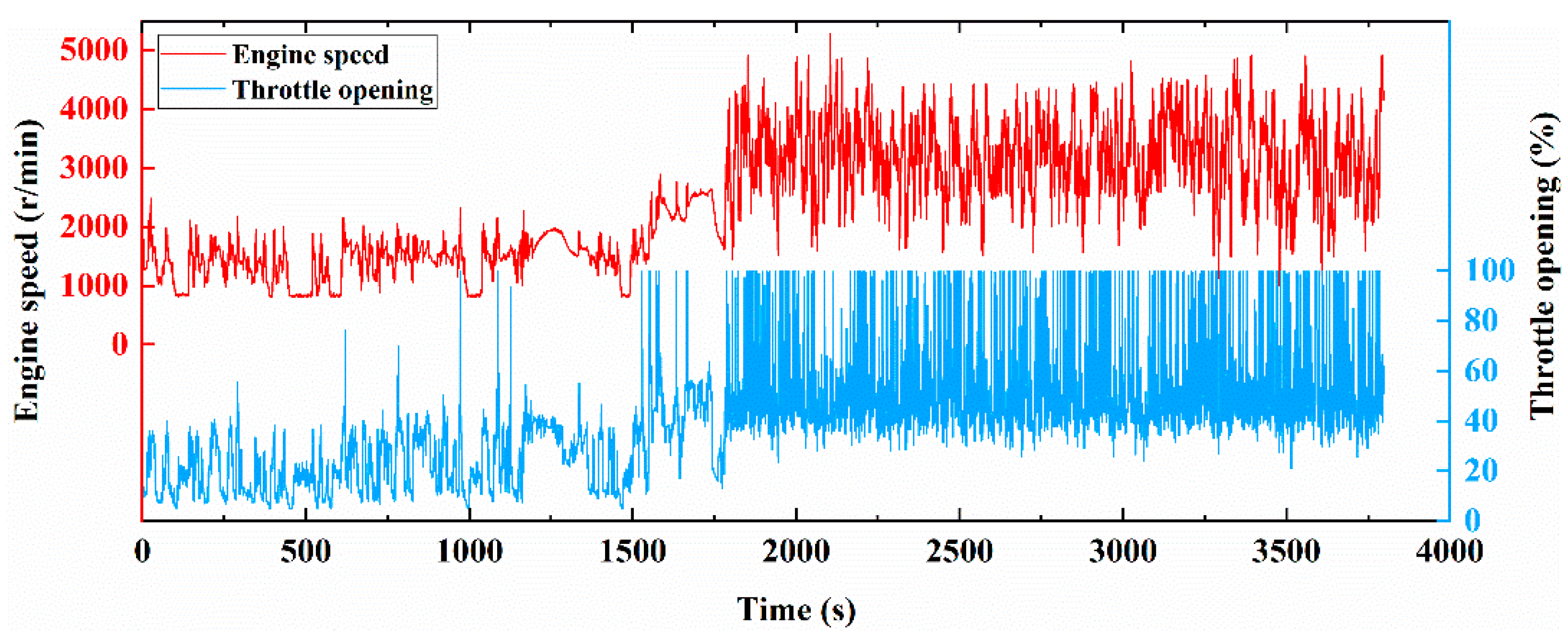
2.1. Data Collection

This paper uses a dataset for model training that includes the following fields: engine speed, torque, throttle valve opening angle, air–fuel ratio, ignition timing, fuel injection pressure, fuel injection pulse width, and exhaust gas soot mass concentration at the TWC outlet. An engine bench test was conducted to collect the data required for the dataset. Figure 1 shows the schematic view of the experimental setup. The arrows indicate the direction of gas flow.

The test engine is a turbocharged 4-cylinder homogeneous GDI engine with a displacement of 1.5 L, a calibrated power of 125 kW, and a compression ratio of 10.5. The test equipment includes an engine bench and a soot mass concentration measurement system. A HORIBA engine bench is used for engine control and bench data collection. AVL 483 is used to measure the soot mass concentration in exhaust gas, where the sampling tube for AVL 483 is set at the TWC outlet. The AVL micro-soot sensor operates on the principle of the photoacoustic effect. Inside the measuring chamber, soot particles in the exhaust gas absorb energy under laser light. This process cyclically heats and cools the surrounding gas, generating sound waves. The intensity of the resulting acoustic signal is directly proportional to the mass concentration of soot, allowing real-time determination of soot mass concentration. The AVL micro-soot sensor offers a broad measurement range and responds rapidly to transient changes in exhaust soot concentration, making it highly suitable for the dynamic operating conditions in this experiment.

The engine operating profile used in the bench test comprises two parts and lasts for 3800 s. The first part is an 1800 s operating profile of engine speed and throttle valve opening angle obtained by a vehicle equipped with the same model engine running the Worldwide Harmonized Light Vehicles Test Cycle (WLTC). In the WLTC cycle, regions with high soot emissions constitute a very small percentage. Nevertheless, accurate prediction of these high soot emissions is indispensable. Low-speed, high-load and high-speed, high-load conditions, characterized by heavy acceleration, are primary contributors to high soot emissions, yet they collectively account for less than 1% of the WLTC. Furthermore, at medium and high-speed, high-load conditions, the elevated temperatures facilitate soot oxidation within the GPF. To ensure the subsequent accuracy of soot load estimation, precise prediction of soot concentration under these operating conditions is crucial. Therefore, this study supplemented the dataset with the second part operating condition to enrich the data and enhance the accuracy of soot concentration prediction. The second part is a 2000 s random operating profile generated from the engine soot mass concentration map. The ratio of high, medium, and low soot mass concentration conditions is set to 7:2:1. The transient condition set is repeated three times, and the total length of the profile is set to 11,400 s. The data were collected at a frequency of one measurement per second, resulting in a dataset comprising 11,400 samples. Where 80% of the dataset, i.e., 9120 s, is used as the training dataset, and 20% of the dataset, i.e., 2280 s, is used as the test dataset. Figure 2 shows the engine operation conditions for data collection. Crucially, the data partitioning ensured that the concentration distributions of both the training and test sets remained consistent. During the test, a warm-up procedure was initiated following engine start-up, and once stable operating conditions were achieved (water temperature reaching 80 °C), the cyclic testing commenced. Data was continuously acquired over three consecutive cycles.

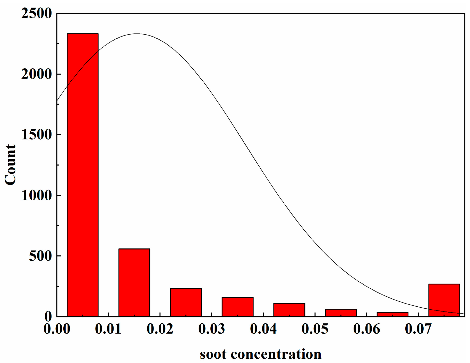
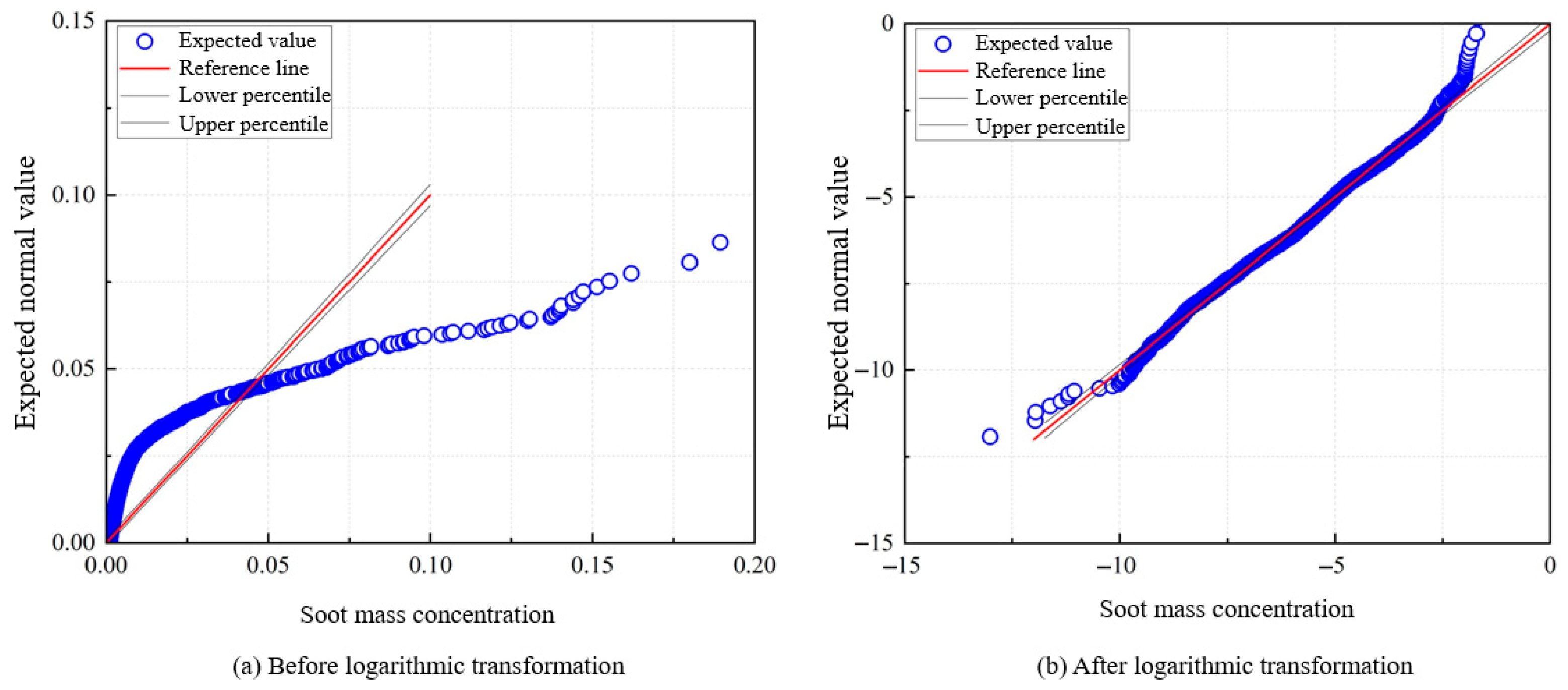
2.2. Data Normalization

In this paper, the min–max normalization method (formula (1)) is used to normalize the collected data:

$$X_{normalization}={\displaystyle \frac{X-Min\left(X\right)}{Max\left(X\right)-Min\left(X\right)}}$$

(1)

where X_{normalization} is the normalization result, X is the value before normalization, and Max and Min represent the maximum and minimum values, respectively, in the dataset before normalization.

Figure 3 presents the concentration distribution plot. It can be observed that while the custom operating conditions supplemented some mid-to-high concentration soot emissions data, the overall dataset remains predominantly composed of low concentrations. The ideal training dataset should comply with the principle of sample balance in statistics, that is to say, the more uniform the sample distribution, the more accurate the model estimation results obtained. Figure 4a shows the quantile plot of soot mass concentration. It is obvious that the sample distribution of the soot mass concentration dataset is not uniform, and may affect the accuracy if directly used as input data. A logarithmic transformation is used to compress the original data, as shown in Figure 4b, bringing it closer to the baseline of a normal distribution.

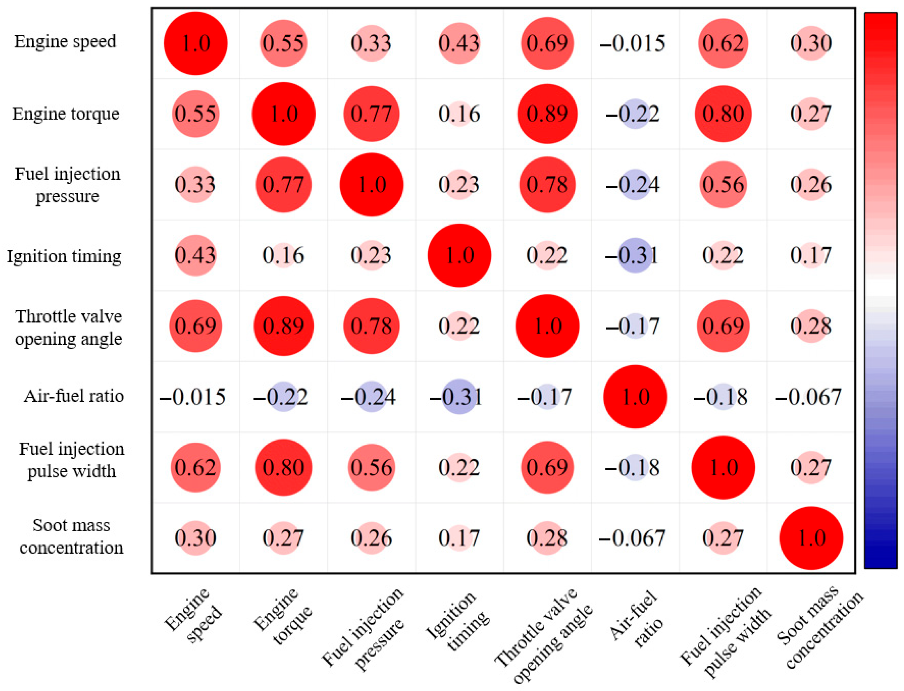
2.3. Data Correlation Analysis

Figure 5 shows the correlation between soot mass concentration and engine operating parameters, i.e., engine speed, engine torque, ignition timing, throttle valve opening angle, air–fuel ratio, fuel injection pressure, and fuel injection pulse width. The correlation coefficients derived from the experimental data are computed as follows:

$$r={\displaystyle \frac{{\sum }_{i=1}^n(x_i-\overline{x})(y_i-\overline{y})}{\sqrt{{\sum }_{i=1}^n{(x_i-\overline{x})}^2}\sqrt{{\sum }_{i=1}^n{(y_i-\overline{y})}^2}}}$$

(2)

It can be seen that the soot mass concentration is positively correlated with engine speed and torque, fuel injection pressure and pulse, ignition timing, and throttle valve opening angle. The correlation between the air–fuel ratio and soot concentration is very low, whereas throttle opening has a strong correlation with engine speed and torque, and fuel injection pressure and pulse. This is due to the fact that the throttle opening adjusts in conjunction with fuel injection, thereby determining engine speed and torque. Therefore, the throttle opening is not needed as an input feature for model training. Thereby, engine speed and torque, fuel injection pressure and pulse, and ignition timing were selected as input data to train the model and to predict the soot mass concentration of the GDI engine.

3. Model Construction and Validation

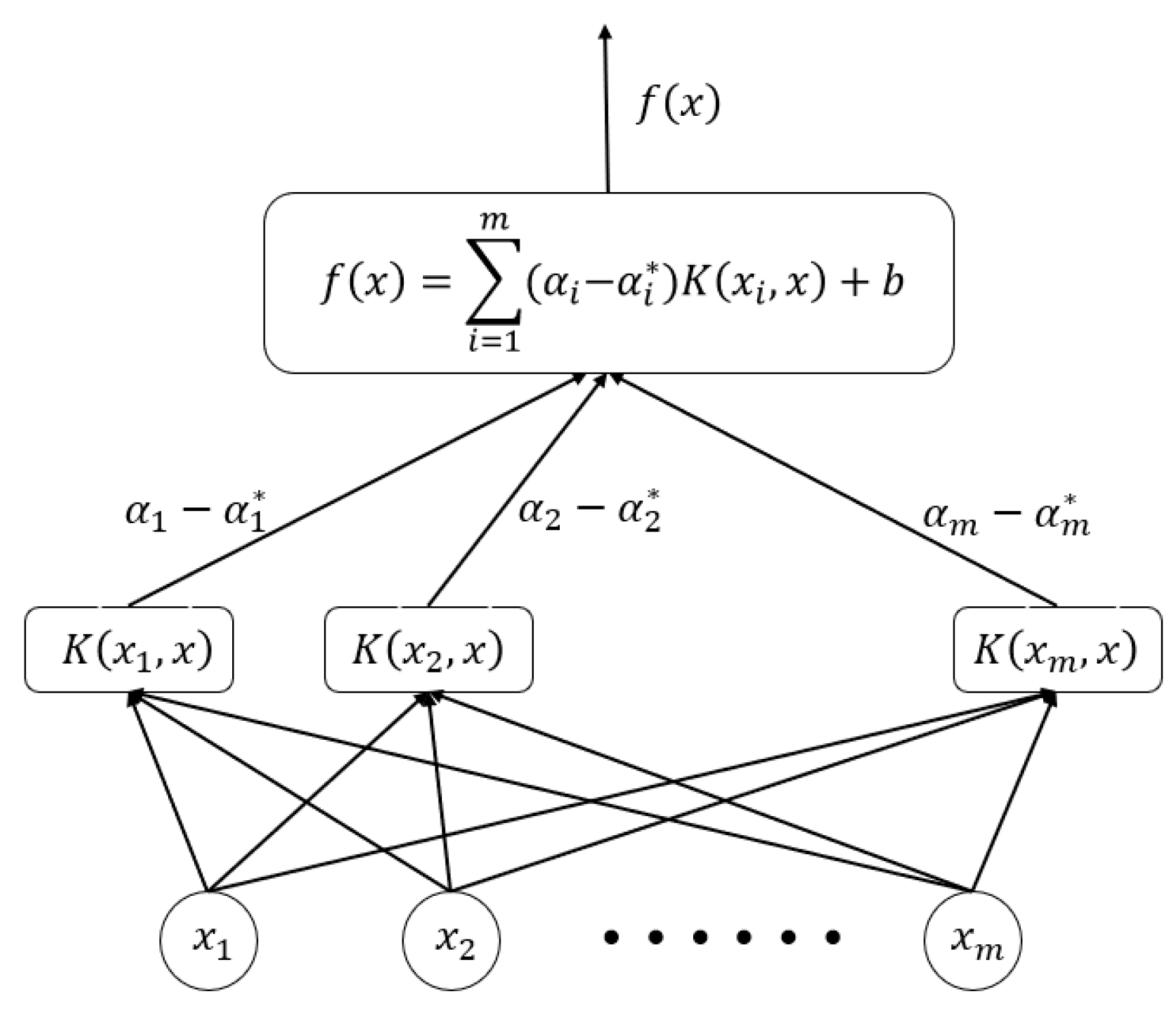
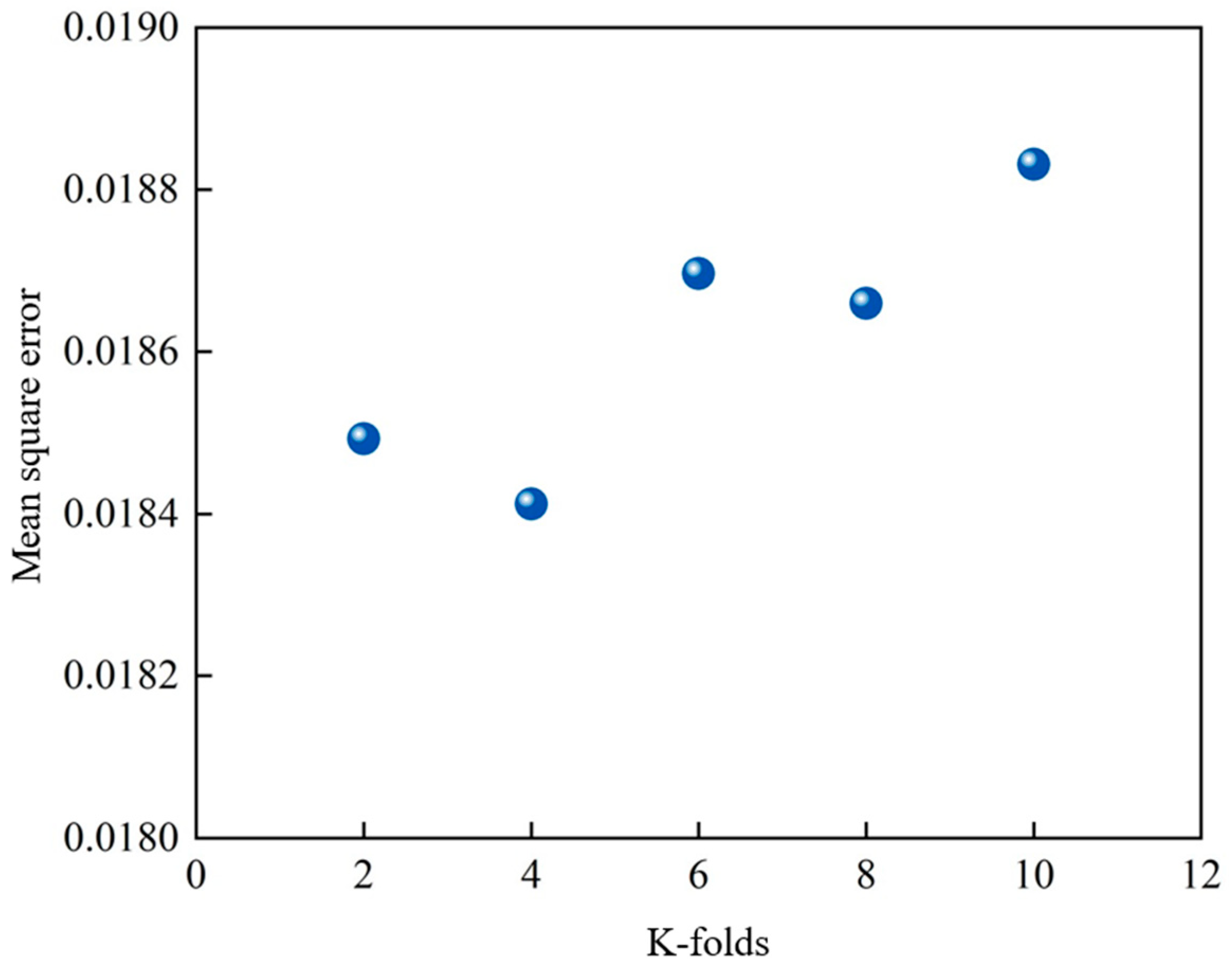
3.1. SVR Model

SVR follows the VC dimension theory and the principle of minimizing structural risk in statistical learning theory, and performs well in the application of classification and regression analysis problems in small sample, nonlinear, and high-dimensional patterns. The principle of SVR is to find a hyperplane, and then implement data regression analysis by minimizing the distance between the hyperplane and the farthest sample point. When given a dataset $T=\left\{\left(x_1,y_1\right),\left(x_2,y_2\right),\left(x_3,y_3\right),\cdots ,\left(x_m,y_m\right)\right\}$ with a size of m × (n + 1), in which the input vector is n-dimensional and the output vector is y, then the optimal hyperplane is established based on the dataset of $\mathrm{g}\left(x\right)=\omega x+b$. Where w is the normal vector to the hyperplane, and b is the bias term. Figure 6 shows the algorithm structure diagram of SVR.

A tolerance deviation, which is represented as ∈, is set based on experience before minimizing the loss function. When the sample falls within the tolerance deviation, no loss is considered. While the loss is included in the loss function if the sample does not fall within the tolerance deviation. The model can then be expressed as minimizing the complexity and the total loss. And, the optimization objective function of SVR can be expressed as:

$$\underset{w,b}{\min }{\displaystyle \frac{1}{2}}{‖W‖}^2+C\sum _{i=1}^1({\xi }_i+{\xi }_i^{*})$$

(3)

where ξ is the slack variable, and C is the penalty factor.

The boundary condition is:

$$s.t.\left\{\begin{array}{c}{y}_i=\omega x-b\le \in +{\xi }_i\\ \omega x+b-y_i\le \in +{\xi }_i^{*}\\ {\xi }_i,{\xi }_i^{*}\ge 0\end{array}\right.$$

(4)

The values of ${\xi }_i$ and ${\xi }_i^{*}$ are:

$$\left\{\begin{array}{c}{\xi }_i=y_i-\left(\omega x+b+\in \right),y_i>\omega x+b+\in \\ {\xi }_i=0, otherwise\end{array}\right.$$

(5)

$$\left\{\begin{array}{c}{\xi }_i^{*}={\left(\omega x+b+\in \right)-y}_i,y_i<\omega x+b-\in \\ {\xi }_i^{*}=0, otherwise\end{array}\right.$$

(6)

Then, a Lagrange function is constructed to minimize the objective function:

$$\begin{array}{cc}\mathrm{L}=& {\displaystyle \frac{1}{2}}{‖W‖}^2+C{\displaystyle \sum _{i=1}^1}\left({\xi }_i+{\xi }_i^{*}\right)-{\displaystyle \sum _{i=1}^1}{\alpha }_i\left({\in +\xi }_i-y_i+\omega x+b\right)\hfill \\ & -{\displaystyle \sum _{i=1}^1}{\alpha }_i^{*}\left(\in +{\xi }_i^{*}+y_i-\omega x-b\right)-{\displaystyle \sum _{i=1}^1}({\eta }_i{\xi }_i+{\eta }_i^{*}{\xi }_i^{*})\hfill \end{array}$$

(7)

s.t. ${\alpha }_i$, ${\alpha }_i^{*}$, ${\eta }_i$, ${\eta }_i^{*}\ge 0$.

Then, the optimization problem is transformed into a dual problem:

$$\left\{\begin{array}{c}\underset{\alpha }{\max }{\displaystyle \sum _{i=1}^m}{\alpha }_i-{\displaystyle \frac{1}{2}}{\displaystyle \sum _{i=1}^m}{\displaystyle \sum _{j=1}^n}{\alpha }_i{\alpha }_j{y}_i{y}_{j}K(x_i,x_j)\\ s.t. 0\le {\alpha }_i\le C,i=1,2,\dots ,m\\ {\displaystyle \sum _{i=1}^m}{\alpha }_i{y}_i=0\end{array}\right.$$

(8)

where α_i is the Lagrange coefficient and not 0, $K(x_i,x_j)$ is the kernel function for the SVR model.

Finally, the regression function of the SVR model is:

$$f\left(x\right)=\sum _{i=1}^m\left({\alpha }_i-{\alpha }_i^{*}\right)K\left(x_i,x\right)+b 0<{\alpha }_i<C$$

(9)

The selection of the kernel function and penalty factor jointly determines the performance of the SVR model. In particular, the kernel function extends the vector inner product space to transform nonlinear regression problems into approximate linear regression problems, and to avoid inner product calculations in high-dimensional feature spaces. The penalty factor is a parameter that imposes corresponding penalties on the ${\omega }^{*}$ point when it deviates from the track and returns the point to the normal region to minimize sample bias. At the same time, ensuring a certain level of expansion capability and meeting the principle of minimizing structural risk in statistics. In this paper, the kernel function is selected as a radial basis function, the stopping tolerance is set to 0.001, and the penalty factor is set to 1.0.

A K-fold cross-validation method is used during SVR model construction. Figure 7 shows the mean square error (MSE) of different K-folds. It can be seen that MSE is minimized at K = 4. So, the K-fold is set to four in the SVR model.

Table 1. MSE, MAE, and R² of the SVR model.

Kernel Function	K-Folds	MSE	MAE	R2
Radial basis function	4	0.018295	0.07249	0.937

lists the MSE, mean absolute error (MAE), and correlation coefficient (R²) of the SVR model constructed in this paper.

Figure 8 compares the SVR prediction and test results of soot mass concentration. The box plotted on the left reflects the distribution of the test data, and the normal curve plotted on the right reflects the density of the data. It can be seen that the data distribution of the prediction and test results is similar, with a little higher median for the estimated results. The data density of the prediction and test results both presents larger values in small soot mass concentrations. The data distribution concentrated area of the test results is slightly smaller than that of the prediction results. The model has a good prediction effect in the range of soot mass concentration 0–0.038 mg/s. Whereas the prediction effect of the SVR model is poor when the soot mass concentration is larger than 0.038 mg/s.

The phenomena observed primarily stem from the SVR model’s high dependency on the training data distribution and its limited extrapolation capability. The model simply lacks sufficient information in the high-concentration range to construct a reliable prediction hyperplane. Essentially, SVR models excel at interpolation within the trained data’s boundaries. The 0.038 mg/s mark likely represents, or is close to, the upper limit of the actual value distribution in the training data. Consequently, with very few data points above this threshold, the model struggles to generate effective predictions. Furthermore, the loss function, by not penalizing errors within the ∈ margin, leads the model to produce a more average prediction rather than fitting each data point precisely [29]. This results in the predicted value distribution appearing broader than the actual values, with a potential slight shift in the center of the concentrated region.

The R² of the SVR model was comparable to that of the previously best-performing prediction model, indicating no significant improvement in prediction accuracy. Consequently, further exploration is required to enhance its precision.

3.2. DNN Model

A neural network is a computational model that simulates the structure and function of a human brain neuron. It consists of multiple layers of neurons and can achieve tasks such as classification, prediction, and recognition through learning and training. A DNN is a neural network consisting of multiple hidden layers that are fully connected to each other. A DNN uses weights and biases between layers to perform nonlinear transformations on input data to represent data features.

Figure 9 shows the structure diagram of the DNN prediction model built in this paper. Considering that predicting soot concentration based on multiple factors is inherently a complex, non-linear problem, a deeper architecture enables the network to progressively extract more sophisticated features, thereby contributing to accurate prediction. Therefore, the DNN prediction model employs a total of five hidden layers. The input layer includes five neurons, i.e., engine speed, torque, fuel injection pulse width, fuel injection pressure, and ignition timing. The output layer is the soot mass concentration at the TWC outlet. Batch size and epoch were set to 256 and 8, respectively. These parameter settings facilitate parallel computing, leading to faster execution speeds. Additionally, the loss calculation for each iteration transforms from a global loss to a local loss, which generally results in better performance compared to traditional methods.

The training process of a DNN mainly consists of three steps. First, the data is unidirectionally transmitted into the neural network. Second, the loss function is calculated. Finally, the deviation between the actual and predicted value is calculated and transferred back to update the weights and biases until the model converges. The learning rate is an important parameter for a DNN model, where a high learning rate may cause the model to fail to converge, while a low learning rate affects the model’s running speed. Figure 10 shows the iterative curve of the training and test sets with different learning rates. It can be seen that the model converges fastest and the convergence curve has no significant fluctuations when the learning rate is 0.01. Therefore, the learning rate is set as 0.01 in this paper.

The function of the activation function in hidden layers is to convert the sum of the input signals from the previous layer into an output signal. And it is the key factor affecting the convergence speed and error of the DNN model. Figure 11 compares the influence of different activation functions on the convergence speed of the DNN model. It can be seen that the ReLU activation function converges quickly and has the smallest error, while the Sigmoid activation function has poor performance and converges after 50 iterations. The tanh activation function has a convergence speed similar to the ReLU activation function but with a higher error. So, the activation function of the DNN model in this paper is selected as ReLU.

Table 2. MSE, MAE, and R² of the DNN model.

Activation Functions	Learning Rate	MSE	MAE	R2
ReLU	0.01	0.01349	0.06328	0.984

lists the MSE, MAE, and R² of the DNN model.

Figure 12 compares the DNN prediction and test results of soot mass concentration. It can be seen that the distribution, median, and data density of the prediction results obtained by the DNN model are similar to those of the test results. While the median of the prediction results is closer to that of the test results, especially within the range of the 25–75% dataset. The DNN model has a good prediction effect in the range of soot mass concentration 0–0.032 mg/s. The correlation coefficient in the training set reached 0.984, but there exist a few negative prediction results due to the overfitting caused by the number of hidden layers.

The paucity of training data in the high-concentration range is fundamentally responsible for this phenomenon. For regions not sufficiently covered in the training set, the DNN’s extrapolation capabilities are typically limited. Furthermore, it is plausible that high-concentration data points were mapped to negative values in the network’s initial layers. Under these conditions, the ReLU activation function will output zero, leading to information loss in subsequent layers and consequently hindering the model’s capacity to learn and predict effectively in the high-concentration domain. The five hidden layers offer substantial learning capacity, which exponentially boosts predictive capability [30]. However, when combined with the chosen batch size and epoch settings, this architecture provides ample opportunity for the model to overfit the training data [31].

The DNN model achieved an R² of 0.984, representing a substantial increase compared to the previous highest prediction model’s R² of 0.932. However, the DNN model exhibited a limited prediction range and suffered from overfitting. Therefore, methods to address these issues in the DNN model need to be investigated.

3.3. Integration Model of SVR and DNN Based on Stacking Algorithm

The integration of different models can effectively reduce the model’s variance, avoid overfitting, and improve the model’s generalization ability [32]. Ensemble learning algorithms primarily include Bagging, Boosting, and Stacking. Bagging operates by sampling with replacement from the training data to create multiple subsets. A sub-model is then trained on each of these subsets, and this process is repeated. Finally, the predictions from these sub-models are combined through voting or averaging to produce a more generalized result [33]. Boosting algorithms, on the other hand, are iterative. The core idea is to focus on misclassified samples from previous training iterations, increasing their weight to ensure they are correctly handled in subsequent steps, thereby sequentially improving model performance [34]. The Stacking algorithm combines the prediction results of multiple models to complete the final output. In specific, the Stacking algorithm typically has a two-layer structure, the first layer consists of multiple base learners, and the output of each base learner is used as a new input for training the meta learner of the second layer. During the training process, the weights of models with better performance will continue to increase, while the performance of models with poor performance is suppressed to obtain more accurate prediction results. And the Stacking algorithm usually uses the K-fold cross-validation method for training to avoid overfitting.

An integration model of SVR and DNN based on the Stacking algorithm is constructed in this paper to improve the prediction accuracy of soot mass concentration. Where both SVR and DNN are used as the base learners, and the linear regressor algorithm is used as the meta learner. Five-fold cross-validation for training is chosen to avoid overfitting. Figure 13 shows the schematic diagram of the Stacking algorithm.

First, the collected dataset is divided into the training set (i.e., training dataset) and the testing set (i.e., test dataset) in a 4:1 ratio, ensuring consistent concentration distributions between the two. Second, the training dataset is further divided into five parts, in which four parts are used as the training dataset (i.e., Train_train) for model training of the base learner (i.e., SVR or DNN), and one part is used as the validation dataset (i.e., Train_Val). There are five training datasets and five validation datasets according to the different composition order of the datasets. It was also ensured that the concentration distribution remained consistent across all five parts. Third, five validation datasets and five test datasets are input into five models, named as model 1-1, model 1-2, model 1-3, model 1-4, and model 1-5, respectively. Then, five prediction results based on validation datasets (i.e., Val_prediction) and five prediction results (i.e., Test_prediction) based on the test dataset are obtained by SVR or DNN, respectively. Fourth, the predicted results of the validation dataset and the test dataset are combined separately to form the next training dataset (i.e., Val_prediction) and the test dataset (i.e., Test prediction). Fifth, test datasets obtained by SVR are combined with the test dataset obtained by DNN to form a new test dataset (i.e., New test set). And the training dataset obtained by SVR and the training dataset obtained by the DNN are combined to form a new training dataset (i.e., New training set). Sixth, the new training and new test datasets are inputted into the meta learner (i.e., linear regressor). Finally, the prediction results are outputted.

Table 3. MSE, MAE, and R² of the integration model of the SVR and DNN model.

Model	MSE	MAE	R2
Stacking	0.00976	0.05948	0.992

lists the MSE, MAE, and R² of the integration model of SVR and DNN-based Stacking algorithm. Figure 14 compares the prediction and test results of soot mass concentration.

It can be seen that the distribution of test and prediction results obtained by the Stacking integration of the SVR and DNN model is relatively concentrated. The model can effectively estimate the soot mass concentration over the entire range of 0–0.07 mg/s, which is larger than that of a single SVR or DNN model. And the overfitting of the DNN model is also avoided.

The improved accuracy of the Stacking model likely stems from the fact that different base models, during their respective learning processes, capture distinct features within the high-concentration regions. The meta-learner is then able to integrate these fragmented and incomplete features. Furthermore, the meta-learner extracts useful information even from the low-confidence predictions of the base learners, thereby achieving accurate predictions in the high-concentration range [35]. Additionally, the Stacking model effectively mitigates overfitting through its inherent ensemble diversity. When a base learner exhibits a tendency to overfit, this is corrected by incorporating predictions from another more stable base learner, thus resolving the overfitting issue observed in the DNN model.

The Stacking model achieved an R² of 0.992, significantly surpassing the previous highest prediction model’s R² of 0.932. This enhancement substantially improves the accuracy of soot concentration prediction, offering a valuable reference for more precise estimation of soot load in GPFs.

3.4. Analysis of Model Differences

When assessing the statistical significance of differences in predictive performance among various models, merely comparing their numerical performance metrics is insufficient, as these discrepancies could simply arise from random fluctuations. Therefore, Analysis of Variance (ANOVA) is essential for conducting a model differentiation analysis. In this study, ANOVA was performed using the MSE values from three models across three cycles.

Table 4. MSE values for these three models over three cycles.

Model	First Cycle	Second Cycle	Third Cycle
SVR	0.01912	0.01746	0.01824
DNN	0.01342	0.01260	0.01446
Stacking	0.00929	0.01065	0.00933

presents the MSE values for these three models over three cycles.

The Sum of Squares Between (SSB) quantifies the variability among the average MSEs of different models, reflecting the overall impact of model selection on performance. Conversely, the Sum of Squares Within (SSW) measures the variability of MSE results within each individual model, representing fluctuations due to random error or unconsidered factors. ANOVA calculations yielded an SSB of 0.0001093 and an SSW of 0.0000043. Furthermore, the calculated F-statistic was 76.018276, with a corresponding P-value of 0.000055, which is less than the significance level of 0.05. This indicates that at least one model’s average performance significantly differs from the others.

To ascertain that the Stacking model significantly outperforms the other two models, post hoc tests were subsequently conducted. This study employed Tukey’s Honestly Significant Difference (HSD) test. The HSD test compares the absolute difference between the mean MSEs of any two models against the calculated HSD value. A difference greater than the HSD value signifies a statistically significant distinction between those two models. The formula for Tukey’s HSD is:

$$HSD=q_{crit}\times \sqrt{{\displaystyle \frac{MSE}{n}}}$$

(10)

Using the Studentized Range q Table with α = 0.05, k = 3, and df_W = 6, a $q_{crit}$ of 4.339 was obtained. This resulted in a final HSD value of 0.00212. The absolute differences in the mean MSE between the Stacking model and the SVR model, and the Stacking model and the DNN model, were 0.00852 and 0.00374, respectively. Both values are greater than the HSD value, thereby confirming a significant difference between the Stacking model and both the SVR and DNN models.

4. Conclusions

This study conducts a soot mass concentration prediction model at the GPF inlet of the GDI engine by using SVR, DNN, and the Stacking integration of SVR and DNN. The soot mass concentration at the GPF inlet is predicted based on engine speed, torque, ignition timing, throttle valve opening angle, fuel injection pressure, and pulse width, and the soot mass concentration at the TWC outlet collected by a GDI engine bench test. Once the soot concentration is accurately estimated, it can be integrated over time and combined with the GPF’s trapping efficiency and soot oxidation rate to calculate the soot load accumulated within the GPF. For example, when the calculated soot load reaches a predefined upper threshold, the ECU controls the engine to conduct regeneration by increasing the exhaust gas temperature through strategies such as adjusting the air–fuel ratio or employing external heaters. The main findings and conclusions are as follows:

(1)

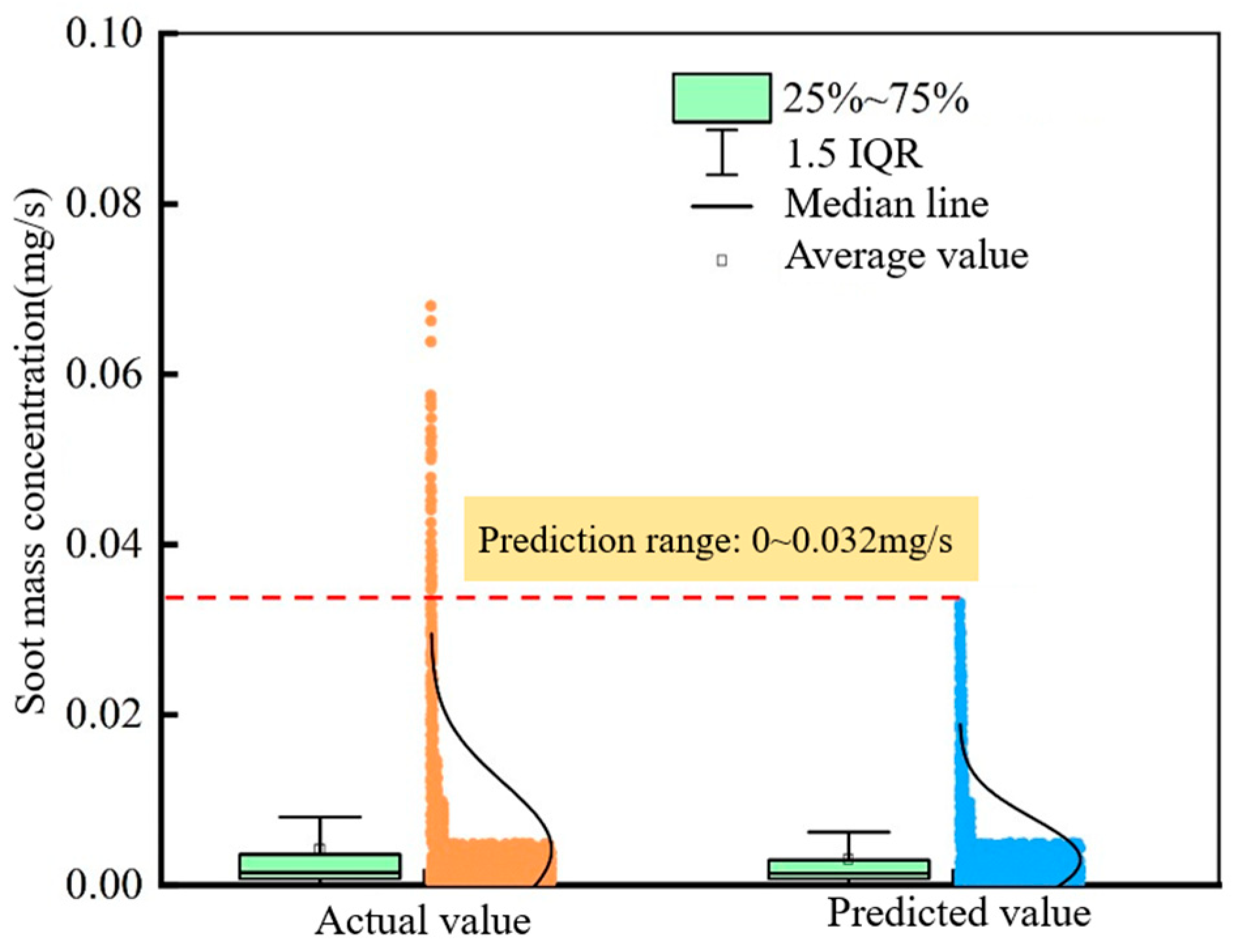
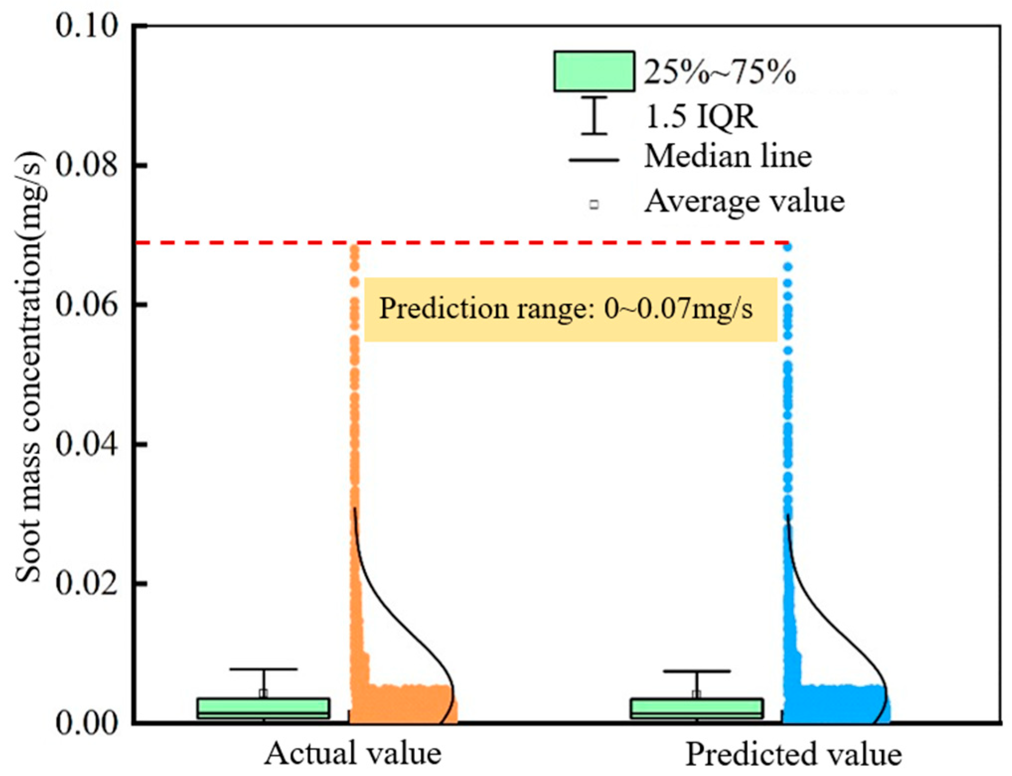
The distribution, median, and data density of prediction results obtained by SVR, DNN, and the Stacking integration of SVR and DNN are all similar to that of the test results. The prediction ranges of soot mass concentration by using SVR, DNN, and the Stacking integration of SVR and DNN are 0–0.038 mg/s, 0–0.030 mg/s, and 0–0.07 mg/s, respectively.

(2)

The R² of the SVR model is 0.937. The median of the prediction results obtained by the SVR model is a little higher the that of the test results, and the concentrated area of the prediction results is slightly smaller than that of the test results. The prediction effect of the SVR model is poor when the soot mass concentration is larger than 0.038 mg/s.

(3)

The R² of the DNN model is 0.984. The median of the prediction results obtained by the DNN model is closer to that of the test results, especially within the range of the 25–75% dataset. And there exist a few negative prediction results on the test dataset due to overfitting.

(4)

The R² of the Stacking integration model of SVR and DNN is 0.992. The integration model can effectively estimate the soot mass concentration over the entire range of 0–0.07 mg/s, and the overfitting of DNN is also avoided.

References

1. Duronio, F.; De Vita, A.; Allocca, L.; Anatone, M. Gasoline direct injection engines—A review of latest technologies and trends. Part 2. Fuel 2020, 265, 116947. [Google Scholar] [CrossRef]
2. Dong, R.; Zhang, Z.; Ye, Y.; Huang, H.; Cao, C. Review of particle filters for internal combustion engines. Processes 2022, 10, 993. [Google Scholar] [CrossRef]
3. de Hartog, J.J.; Hoek, G.; Peters, A.; Timonen, K.L.; Ibald-Mulli, A.; Brunekreef, B.; Tiittanen, P.; Kreyling, W.; Kulmala, M. Effects of fine and ultrafine particles on cardiorespiratory symptoms in elderly subjects with coronary heart disease: The ULTRA study. Am. J. Epidemiol. 2003, 157, 613–623. [Google Scholar] [CrossRef] [PubMed]
4. Wang, J.; Yan, F.; Fang, N.; Yan, D.; Zhang, G.; Wang, Y.; Yang, W. An experimental investigation of the impact of washcoat composition on gasoline particulate filter (GPF) performance. Energies 2020, 13, 693. [Google Scholar] [CrossRef]
5. Komori, A.; Sato, S.; Oryoji, K.; Koiwai, R. Study on Estimation Logic of GPF Temperature and Amount of Residual Soot. Int. J. Automot. Eng. 2021, 12, 9–15. [Google Scholar] [CrossRef] [PubMed]
6. Kamimoto, T.; Murayama, Y.; Minagawa, T.; Minami, T. Light scattering technique for estimating soot mass loading in diesel particulate filters. Int. J. Engine Res. 2009, 10, 323–336. [Google Scholar] [CrossRef]
7. Tiwari, A.; Durve, A.; Barman, J.; Srinivasan, P. Evaluation of Different Methodologies of Soot Mass Estimation for Optimum Regeneration Interval of Diesel Particulate Filter (DPF); SAE Technical Paper No. 2021-26-0208; SAE International: Warrendale, PA, USA, 2021. [Google Scholar]
8. Cheng, X.; Ren, F.; Gao, Z.; Zhu, L.; Huang, Z. Synergistic effect analysis on sooting tendency based on soot-specialized artificial neural network algorithm with experimental and numerical validation. Fuel 2022, 315, 122538. [Google Scholar] [CrossRef]
9. Alonso, J.M.; Alvarruiz, F.; Desantes, J.M.; Hernandez, L.; Hernandez, V.; Molto, G. Combining Neural Networks and Genetic Algorithms to Predict and Reduce Diesel Engine Emissions. IEEE Trans. Evol. Comput. 2007, 11, 46–55. [Google Scholar] [CrossRef]
10. Ghanbari, M.; Najafi, G.; Ghobadian, B.; Mamat, R.; Noor, M.M.; Moosavian, A. Support vector machine to predict diesel engine performance and emission parameters fueled with nano-particles additive to diesel fuel. IOP Conf. Ser. Mater. Sci. Eng. 2015, 100, 012069. [Google Scholar] [CrossRef]
11. Arora, V.; Mahla, S.K.; Leekha, R.S.; Dhir, A.; Lee, K.; Ko, H. Intervention of Artificial Neural Network with an Improved Activation Function to Predict the Performance and Emission Characteristics of a Biogas Powered Dual Fuel Engine. Electronics 2021, 10, 584. [Google Scholar] [CrossRef]
12. Seunghyup, S.; Jong-Un, W.; Minjeong, K. Comparative research on DNN and LSTM algorithms for soot emission prediction under transient conditions in a diesel engine. J. Mech. Sci. Technol. 2023, 37, 2023. [Google Scholar] [CrossRef]
13. Liao, W.R.; Shi, J.H.; Li, G.X. CRDI Engine Emission Prediction Models with Injection Parameters Based on ANN and SVM to Improve the SOOT-NOx Trade-Off. J. Appl. Fluid Mech. 2023, 16, 2041–2053. [Google Scholar] [CrossRef]
14. Kumar, A.N.; Kishore, P.; Raju, K.B.; Ashok, B.; Vignesh, R.; Jeevanantham, A.; Nanthagopal, K.; Tamilvanan, A. Decanol proportional effect prediction model as additive in palm biodiesel using ANN and RSM technique for diesel engine. Energy 2020, 213, 119072. [Google Scholar] [CrossRef]
15. Jayaprakash, B.; Wilmer, B.; Northrop, W.F. Initial Development of a Physics-Aware Machine Learning Framework for Soot Mass Prediction in Gasoline Direct Injection Engines. SAE Int. J. Adv. Curr. Pract. Mobil. 2023, 6, 2005–2020. [Google Scholar]
16. Pu, Y.-H.; Reddy, J.K.; Samuel, S. Machine learning for nano-scale particulate matter distribution from gasoline direct injection engine. Appl. Therm. Eng. 2017, 125, 335–345. [Google Scholar] [CrossRef]
17. Stangierska, M.; Bajwa, A.; Lewis, A.; Akehurst, S.; Turner, J.; Leach, F. Ensemble Machine Learning Techniques for Particulate Emissions Estimation from a Highly Boosted GDI Engine Fuelled by Different Gasoline Blends; 2024-01-4306; SAE International: Warrendale, PA, USA, 2024. [Google Scholar]
18. Chu, H.; Xiang, L.; Nie, X.; Ya, Y.; Gu, M. Laminar burning velocity and pollutant emissions of the gasoline components and its surrogate fuels: A review. Fuel 2020, 269, 117451. [Google Scholar] [CrossRef]
19. Shuai, S.; Ma, X.; Li, Y.; Qi, Y.; Xu, H. Recent Progress in Automotive Gasoline Direct Injection Engine Technology. Automot. Innov. 2018, 1, 95–113. [Google Scholar] [CrossRef]
20. Yin, Z.; Liu, S.; Tan, D.; Zhang, Z.; Wang, Z.; Wang, B. A review of the development and application of soot modelling for modern diesel engines and the soot modelling for different fuels. Process Saf. Environ. Prot. 2023, 178, 836–859. [Google Scholar] [CrossRef]
21. Maricq, M.M. Engine, aftertreatment, fuel quality and non-tailpipe achievements to lower gasoline vehicle PM emissions: Literature review and future prospects. Appl. Energy 2023, 886, 161225. [Google Scholar] [CrossRef] [PubMed]
22. Mohsin, R.; Chen, L.F.; Felix, L.; Ding, S.T. A Review of Particulate Number (PN) Emissions from Gasoline Direct Injection (GDI) Engines and Their Control Techniques. Energies 2018, 11, 1417. [Google Scholar] [CrossRef]
23. Qian, Y.; Li, Z.; Yu, L.; Wang, X.; Lu, X. Review of the state-of-the-art of particulate matter emissions from modern gasoline fueled engines. Appl. Energy 2019, 238, 1269–1298. [Google Scholar] [CrossRef]
24. Hua, Y.; Liu, F.; Wu, H.; Lee, C.-F.; Li, Y. Effects of alcohol addition to traditional fuels on soot formation: A review. Int. J. Engine Res. 2021, 22, 1395–1420. [Google Scholar] [CrossRef]
25. Catapano, F.; Di Iorio, S.; Luise, L.; Sementa, P.; Vaglieco, B.M. Influence of ethanol blended and dual fueled with gasoline on soot formation and particulate matter emissions in a small displacement spark ignition engine. Fuel 2019, 245, 253–262. [Google Scholar] [CrossRef]
26. Koch, S.; Hagen, F.P.; Büttner, L.; Hartmann, J.; Velji, A.; Kubach, H.; Koch, T.; Bockhorn, H.; Trimis, D.; Suntz, R. Influence of Global Operating Parameters on the Reactivity of Soot Particles from Direct Injection Gasoline Engines. Emiss. Control Sci. Technol. 2022, 8, 9–35. [Google Scholar] [CrossRef]
27. Jiao, Q.; Rolf, D.R. The Effect of Operating Parameters on Soot Emissions in GDI Engines; 2015-01-1071; SAE International: Warrendale, PA, USA, 2015. [Google Scholar]
28. Xing, J.; Shao, L.; Zheng, R.; Peng, J.; Wang, W.; Guo, Q.; Wang, Y.; Qin, Y.; Shuai, S.; Hu, M. Individual particles emitted from gasoline engines: Impact of engine types, engine loads and fuel components. J. Clean. Prod. 2017, 149, 461–471. [Google Scholar] [CrossRef]
29. Alex, J.; Bernhard, S. A tutorial on support vector regression. Stat. Comput. 2004, 14, 199–222. [Google Scholar] [CrossRef]
30. Yoshua, B.; Aaron, C.; Pascal, V. Representation Learning: A Review and New Perspectives. IEEE Trans. Pattern Anal. Mach. Intell. 2013, 35, 1798–1828. [Google Scholar] [CrossRef] [PubMed]
31. Keskar, N.S.; Mudigere, D.; Nocedal, J.; Smelyanskiy, M.; Tang, P.T.P. On large-batch training for deep learning: Generalization gap and sharp minima. In Proceedings of the 5th International Conference on Learning Representations, ICLR 2017-Conference Track Proceedings, Toulon, France, 24–26 April 2017. [Google Scholar]
32. Wolpert, D.H. Stacked generalization. Neural Netw. 1992, 5, 241–259. [Google Scholar] [CrossRef]
33. Breiman, L. Bagging predictors. Mach. Learn. 1996, 24, 123–140. [Google Scholar] [CrossRef]
34. Freund, Y.; Schapire, R.E. A desicion-theoretic generalization of on-line learning and an application to boosting. Eur. Conf. Comput. Learn. Theory 1997, 55, 119–139. [Google Scholar]
35. Ting, K.; Witten, I. Issues in Stacked Generalization. J. Articial Intell. Res. 1999, 10, 271–289. [Google Scholar] [CrossRef]
Figure 1. Engine test bench schematic.
Energies 18 03861 g001
Figure 2. Engine operation conditions for data collection.
Energies 18 03861 g002
Figure 3. Concentration distribution plot.
Energies 18 03861 g003
Figure 4. Quantile plot of the soot mass concentration dataset.
Energies 18 03861 g004
Figure 5. Thermogram of correlation between soot mass concentration and engine operation parameters.
Energies 18 03861 g005
Figure 6. The algorithm structure diagram of SVR.
Energies 18 03861 g006
Figure 7. MSE of different K-folds.
Energies 18 03861 g007
Figure 8. SVR prediction and test results of soot mass concentration.
Energies 18 03861 g008
Figure 9. Structure diagram of the DNN.
Energies 18 03861 g009
Figure 10. Iterative curve of the training and validation sets with different learning rates.
Energies 18 03861 g010
Figure 11. Convergence speed and error of different activation functions.
Energies 18 03861 g011
Figure 12. DNN prediction and test results of soot mass concentration.
Energies 18 03861 g012
Figure 13. Schematic diagram of the Stacking algorithm.
Energies 18 03861 g013
Figure 14. Integration model prediction and test results of soot mass concentration.
Energies 18 03861 g014