The Impact of Wind Speed on Electricity Prices in the Polish Day-Ahead Market Since 2016, and Its Applicability to Machine-Learning-Powered Price Prediction

Abstract

The rising share of wind generation in power systems, driven by the need to decarbonise the energy sector, is changing the relationship between wind speed and electricity prices. In the case of Poland, this relationship has not been thoroughly investigated, particularly in the aftermath of the restrictive legal changes introduced in 2016, which halted numerous onshore wind investments. Studying this relationship remains necessary to understand the broader market effects of wind speed on electricity prices, especially considering evolving policies and growing interest in renewable energy integration. In this context, this paper analyses wind speed, wind generation, and other relevant datasets in relation to electricity prices using multiple statistical methods, including correlation analysis, regression modelling, and artificial neural networks. The results show that wind speed is a significant factor in setting electricity prices (with a correlation coefficient reaching up to −0.7). The findings indicate that not only is it important to include wind speed as an electricity price indicator, but it is also worth investing in wind generation, since higher wind output can be translated into lower electricity prices. This study contributes to a better understanding of how natural variability in renewable resources translates into electricity market outcomes under policy-constrained conditions. Its innovative aspect lies in combining statistical and machine learning techniques to quantify the influence of wind speed on electricity prices, using updated data from a period of regulatory stagnation.

1. Introduction

Wind energy is crucial in the global energy transition towards carbon neutrality. During the 2015 UN Climate Change Conference, the Paris Agreement was signed, aiming to limit the rise in Earth’s surface temperature to 1.5 °C [1]. One of the most important causes of global warming is greenhouse gas emissions [2]; hence, current efforts are prioritised to reduce them. To decrease emissions and even halt them entirely by 2050, fossil fuels, such as hard coal and lignite, are being replaced by environmentally friendly renewable energy sources (RESs). These efforts have led to a significant reduction in net greenhouse gas emissions in the EU-27, dropping below 3000 MtCO₂e in 2024 [3]. Among RESs, wind and solar are the most widely recognised, with wind power providing more electricity as of 2023 [4]. Globally, wind energy accounted for 7.8% of electricity generation in 2023, up 0.5 percentage points compared to the previous year. This share was even higher in Europe, reaching 12.3%.

Similarly to global efforts, Poland is also intensifying its transition towards a more renewable energy mix [5]. The current EU goal is to achieve a 42.5% RES share by 2030, as set by Directive 2023/2413 [6]. In line with this, the latest version of the Polish National Energy and Climate Plan sets a national target of 32.6% RESs in final energy consumption [7]. Wind energy is one of the most widely used renewable energy sources in Poland due to its efficiency, scalability, and decreasing costs. In 2023, installed onshore wind capacity reached 8.98 GW, generating 35.208 TWh of electricity, almost 8 TWh more than the previous year [8]. By 2030, onshore and offshore wind farms are expected to contribute 19 and 5.9 GW, respectively, to the installed capacity [7]. As such, wind farms are expected to be a driving factor in achieving carbon-neutral electricity production.

The first wind turbine was connected to the Polish power system in 2002 [9], but early development was hindered by a lack of clear regulations and financial incentives. After joining the European Union in 2004, Poland became subject to EU climate and energy policies, including a target of 7.5% RESs in final consumption by 2010 [10]. According to Ref. [11], between 2005 and 2015, wind capacity increased by an average of 489.5 MW annually, driven by strong market incentives and contributing significantly to Poland’s progress towards EU climate goals (Figure 1).

According to Refs. [13,14], Polish regulations underwent significant changes regarding wind farms in 2016. In response to concerns raised by people living in close proximity to wind turbines, a so-called “10H rule” came into force. The rule stated that no wind turbine could be placed closer than ten times its height to any residential buildings and protected areas, such as national parks [15]. This regulation effectively excluded between 93.1% and 97.5% of Polish territory as potential wind farm locations (depending on the scenario), as the government saw a greater concern in local populations’ comfort, rather than energy sector development. Moreover, between 89% and 97% of wind turbines built before the enactment were located in the excluded zones [11,16,17]. These changes led to a massive, three-year-long halt in the wind energy sector development, during which the yearly increase in 2017, 2018, and 2019 did not even reach 1%.

In 2023, new legislation allowed municipalities to apply exceptions to the 10H rule through local spatial development plans, provided that a minimum distance of 700 metres is maintained [17]. This change aimed to stimulate wind investment and enable local-level decision-making. While the full market response is still developing, the legal shift has already stimulated renewed interest in onshore wind projects.

1.1. Literature Review

Due to the ever-growing renewable energy production, combined with climate and other regional or national conditions, the understanding of its impact on electricity prices in the day-ahead market is constantly challenged. Jonsson et al. (2013) [18] proposed a two-step statistical methodology for forecasting electricity prices accounting for wind power predictions. Using data spanning from 2008 to 2011 from the Western Danish price area, it was concluded that accounting for wind power with adaptive parameter estimation is beneficial to electricity price predictions and could be integrated into other, less wind-focused markets. Branucci Martinez-Anido et al. (2016) [19] used a PLEXOS simulation engine to develop a model of electricity prices in New England, which included wind data as the input and achieved an overall accuracy of more than 90%. They concluded that as electricity prices decrease, their volatility increases with a higher level of wind penetration.

In 2013, Mulder and Scholtens analysed the impact of renewable energy on electricity prices in the Netherlands and concluded that the Dutch market was not significantly affected by the growth of the renewable energy sector [20]. Ketterer conducted a similar analysis on the German market in 2014. The study showed that intermittent wind power generation decreases the wholesale electricity price and increases its volatility [21]. Branucci Martinez-Anido et al. (2016) came to the same conclusion for the New England region in the United States of America [19]. These findings highlight the broader trend observed across various energy markets, where the increasing share of renewables, particularly wind energy, leads to a reduction in electricity prices while simultaneously introducing greater price volatility.

Badyda et al. (2017) [22] analysed the impact of wind on electricity prices in several European countries and found that both power demand and electricity prices are highly dependent on weather conditions, although wind speeds are highly unpredictable. It was also concluded that wind farm generation had a smaller impact on electricity prices in Poland than in France or Italy because wind power did not contribute significantly to the Polish Power System in the analysed years.

According to the findings of the reviewed publications, regional electricity markets differ, especially considering different energy mixes, energy policies, support mechanisms, and geographical locations. Considering conditions in Poland, Pieczarko et al. (2016) [11] analysed spot electricity prices in relation to wind power generation, using data from 2013 to 2015. It was shown that the majority of average daily prices above 180 PLN/MWh occurred only when wind power generation dropped below 1000 MWh. Furthermore, most prices above 200 PLN/MWh were recorded only when wind power generation was around 500 MWh or lower. The impact of wind generation on the incremental clearing price in the Balancing Market was examined by Miller et al. (2015) [14] by determining the nature of this correlation. It was shown that wind generation exceeding 20% of the planned demand has a direct impact on the incremental clearing price.

The aforementioned studies lacked insight into the specificity of the Polish energy market, which is crucial due to Poland’s energy mix, high reliance on coal, and the transitional challenges it faces in aligning with EU decarbonisation targets. Research conducted in other countries takes into account different geographical and environmental characteristics, making direct comparisons difficult or even impossible. Other studies, when they did consider the Polish context, such as Igliński et al. (2015) [23], Gnatowska et al. (2019) [24], and Brzezińska-Rawa et al. (2014) [25], used older data and no prediction models, which makes them less relevant to the current situation. These differences may become even more apparent when considering the impact of the 2020 global pandemic [26] and the ongoing Russian–Ukrainian war that began in 2022 [27].

1.2. Study Contribution

The literature review shows that the impact of certain conditions (both human-dependent and natural) on electricity prices in Poland over the years remains largely unexplored. Previous studies often focused on strictly mathematical and computational analyses, while this study contributes by providing a machine learning context. Machine learning models are capable of outperforming classical forecasting models, and understanding the impact of wind speed input on their accuracy may prove beneficial. As a result, this article aims to examine and understand the dependencies among known electricity production and energy pricing factors, with a particular focus on directions for energy price forecasting, which may support improved investment decisions and energy policy design.

To achieve this, various datasets concerning electricity prices and wind energy generation in Poland in the last eight years were collected and thoroughly analysed. This paper provides a novel and comprehensive analysis of the multiple factors influencing electricity in Poland’s day-ahead market, accounting for an evolving regulatory framework, increasing renewable penetration, and recent external shocks such as the COVID-19 pandemic and the Russian–Ukrainian war.

A key contribution of this research is the integration of historical wind generation data with market price trends, enabling a better understanding of how the growing role of renewable energy sources affects market behaviour. These findings may inform future research on electricity price forecasting in countries undergoing energy transition and offer insights that could support ongoing discussions on energy market design.

The remainder of the paper is organised as follows. Section 2 presents the tools and models developed and employed for analysing gathered data, as well as the data itself. Section 3 presents and discusses the results, and finally, Section 4 concludes the study.

2. Materials and Methods

This section outlines the materials and methods employed for data preprocessing, analysis, and machine learning model development. Figure 2 illustrates an overview of the entire process, which is explained in detail later. Data preprocessing is crucial to ensure data quality and accuracy in later steps, while the analysis provides answers to the aforementioned research problem. A machine learning model is used to confirm the identified dependencies and implement them in practice.

As shown in Figure 2, electricity prices and demand, alongside wind farm capacity, generation, and wind speed, were used as inputs for statistical analysis, regression models, and machine learning models. The data was then processed through these three paths, which resulted in electricity price prediction and electricity prices (wind speed dependency indicators). These were used to draw recommendations regarding wind farm development in Poland.

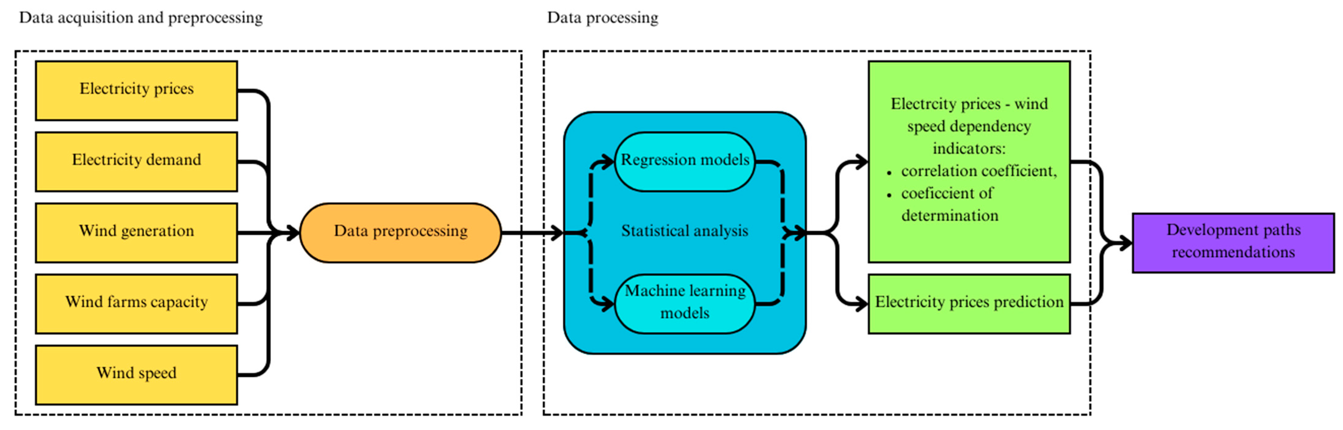
2.1. Data Acquisition and Preprocessing

Retrieved datasets varied in their layouts. The day-ahead market dataset was divided into four columns, that is, price and volume for Fixing I and II, respectively [28]. Rows contained values divided on an hourly basis from 1 January 2016 to 4 December 2024. Other datasets were later adjusted to this one, as it served as a basis for machine learning predictions. Hourly electricity demand and wind generation data were only available from 1 January 2016 to 14 June 2024, because on that day, the Transmission System Operator (TSO) changed the time basis of data acquisition.

The electricity price in the Polish day-ahead market is set according to a merit order, which is a ranking of all offers submitted by the electricity producers from the lowest to the highest. The prices offered typically reflect the variable cost of operating these units. To meet the rising demand, more expensive units must be turned on, which causes the overall price to increase. The merit order is illustrated in Figure 3, in which renewable, cogeneration, and industrial units have the lowest operational costs, whereas conventional units have increasingly higher operational costs, ranging from lignite-fired to natural gas-fired power plants.

The demand dataset contained generation data from the dispatchable and non-dispatchable units, synchronous and asynchronous cross-border exchange data, while the RES dataset contained both wind and solar generation data. The breakdown of electricity generation from 2016 is presented in Figure 4. While regulatory barriers have hindered the development of onshore wind since 2016, they have simultaneously encouraged the growth of small-scale photovoltaic installations [29,30].

The daily average electricity price over time can be seen in Figure 5. Until the first half of 2021, the electricity price remained relatively stable at around 250 PLN/MWh, although a slight decrease was observed in the first half of 2020. Prices in later months reflect the European energy crisis caused by the Russian invasion of Ukraine and the following sanctions. The situation began to stabilise in late 2022.

Two different wind speed datasets were used. One consisted of the daily measurements from all available weather stations in Poland, which also contained the cloud coverage and temperature data from 1 January 2016 to 30 June 2024 (adjusted for the demand and generation datasets) [32]. The other was an hourly reanalysis at the coordinates of some of the largest wind farms in Poland. This was the only dataset not available in Comma-Separated Values (.csv) format, but rather in a General Regularly-distributed Information in Binary form (GRIB) format, which required additional conversion [33]. The wind capacity factor per NUTS 2 region is presented in Figure 6. Since the wind speed data used in subsequent analysis was averaged from reanalysis data points corresponding to the locations of the largest wind farms, the analysed areas naturally overlapped with regions exhibiting the highest capacity factors. In particular, this included areas in northwestern Poland, where average capacity factors ranged from 0.3 to 0.32.

The data used in this study were sourced from multiple governmental and non-governmental institutions to ensure a comprehensive analysis of electricity prices and renewable energy development in Poland. While some datasets were freely accessible, others required access through specialised platforms. Historical pricing and generation data were obtained from Energy Instrat [28], which provides open-access energy market data collected from the day-ahead energy market and the Transmission System Operator (PSE SA, [35]). The Polish Transmission System Operator provided data on demand and generation [35]. Historical wind capacity installed data were obtained from Energy Instrat [31]. Additionally, climate data were retrieved from the Institute of Meteorology and Water Management [32], as well as from ERA5 CDS [33].

Data was mostly analysed using the open-source programming language Python (3.11.0, Python Software Foundation, Wilmington, DE, USA), along with several specialised libraries. The pandas library was used for data processing and analysis, while numpy facilitated operations on multi-dimensional arrays and matrices, as well as high-level mathematical functions. Scipy is a commonly used Python library that provides fundamental algorithms for scientific computing, such as optimisation, interpolation, and other problem classes. Keras is an open-source artificial neural network library integrated into the TensorFlow software library. Finally, the statsmodels library was used for regression models, and the matplotlib library for generating plots.

Before analysis, the data had to be cleaned and pre-processed to ensure its consistency and accuracy. Data cleaning was performed using Python and the pandas library, in which missing values were handled appropriately to prevent errors in calculations. Depending on the specific dataset, missing values were replaced with either interpolated values or the most recent valid values. To facilitate time series analysis, all indices were converted to a datetime object, representing each hour since 1 January 2016 01:00:00. Finally, all individual datasets were merged into a single, unified dataset.

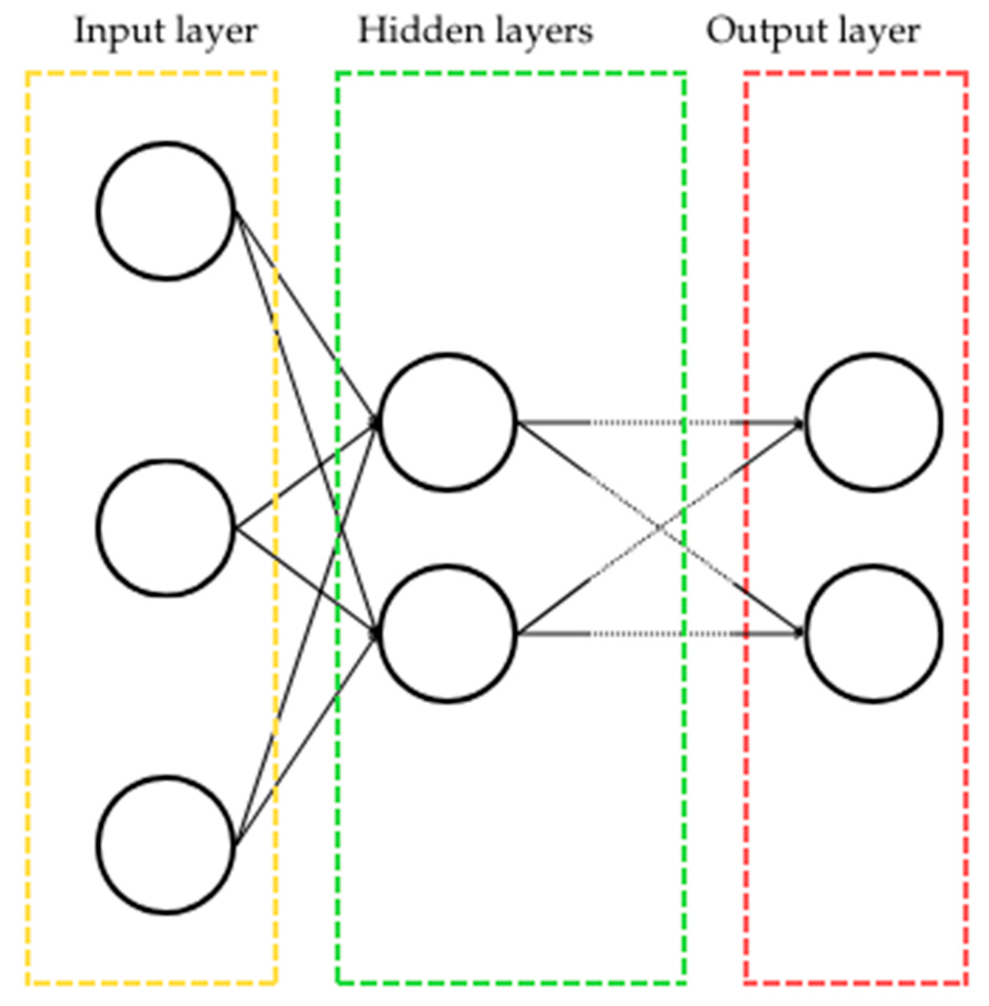
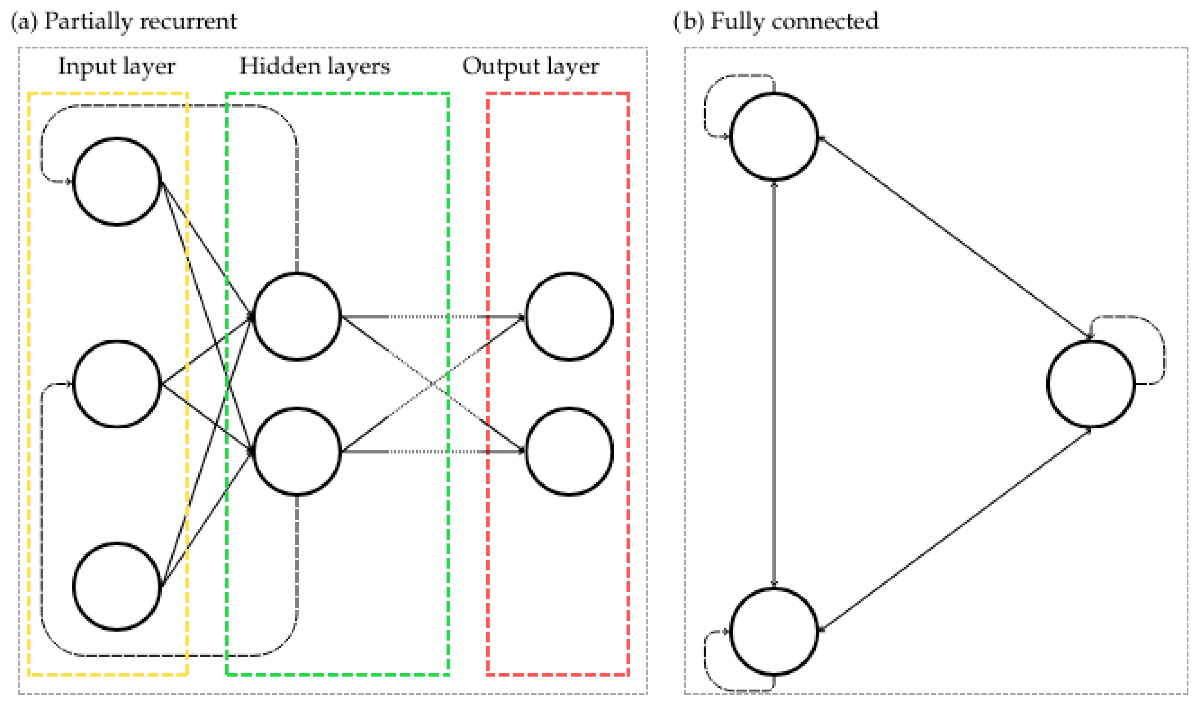
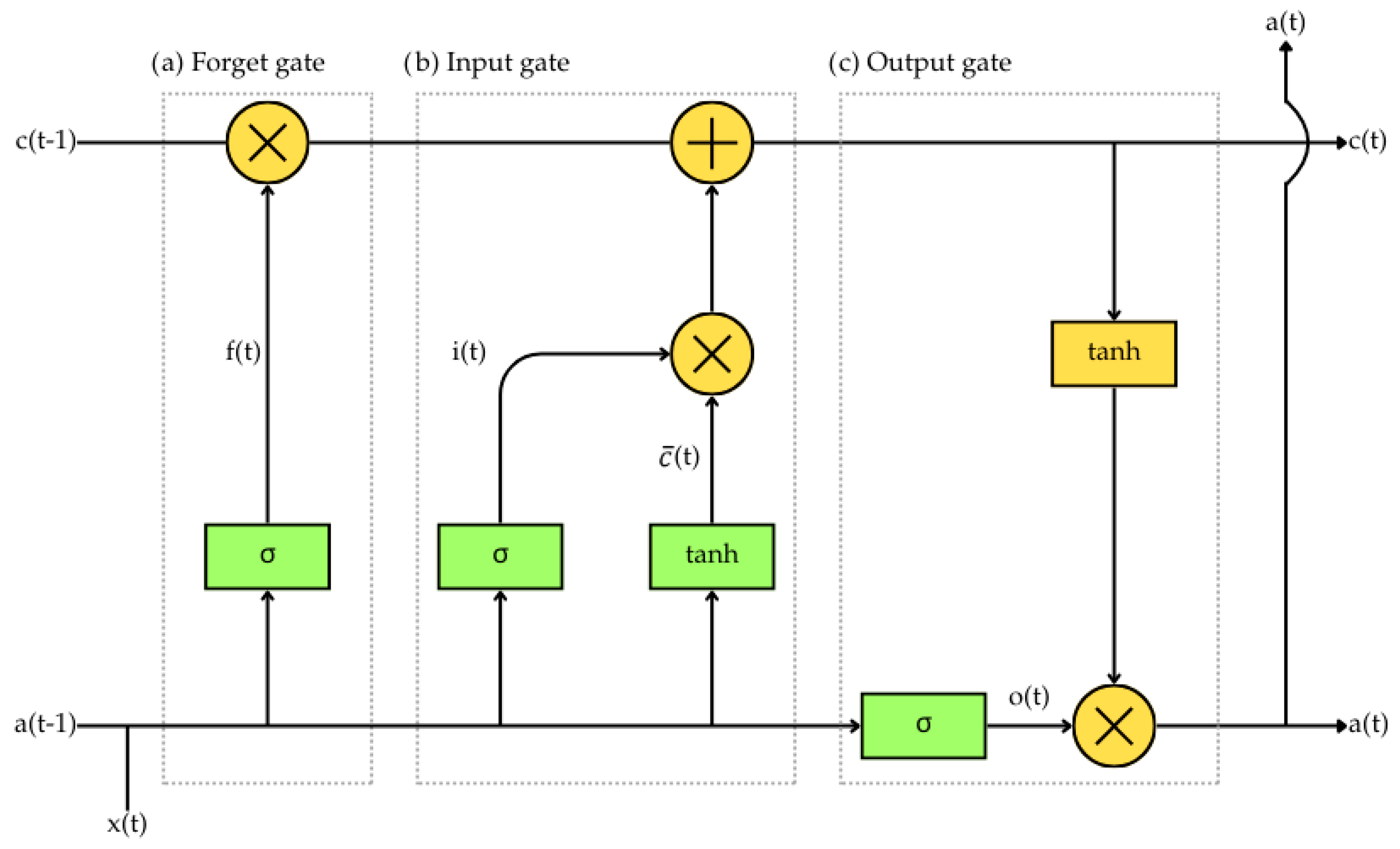
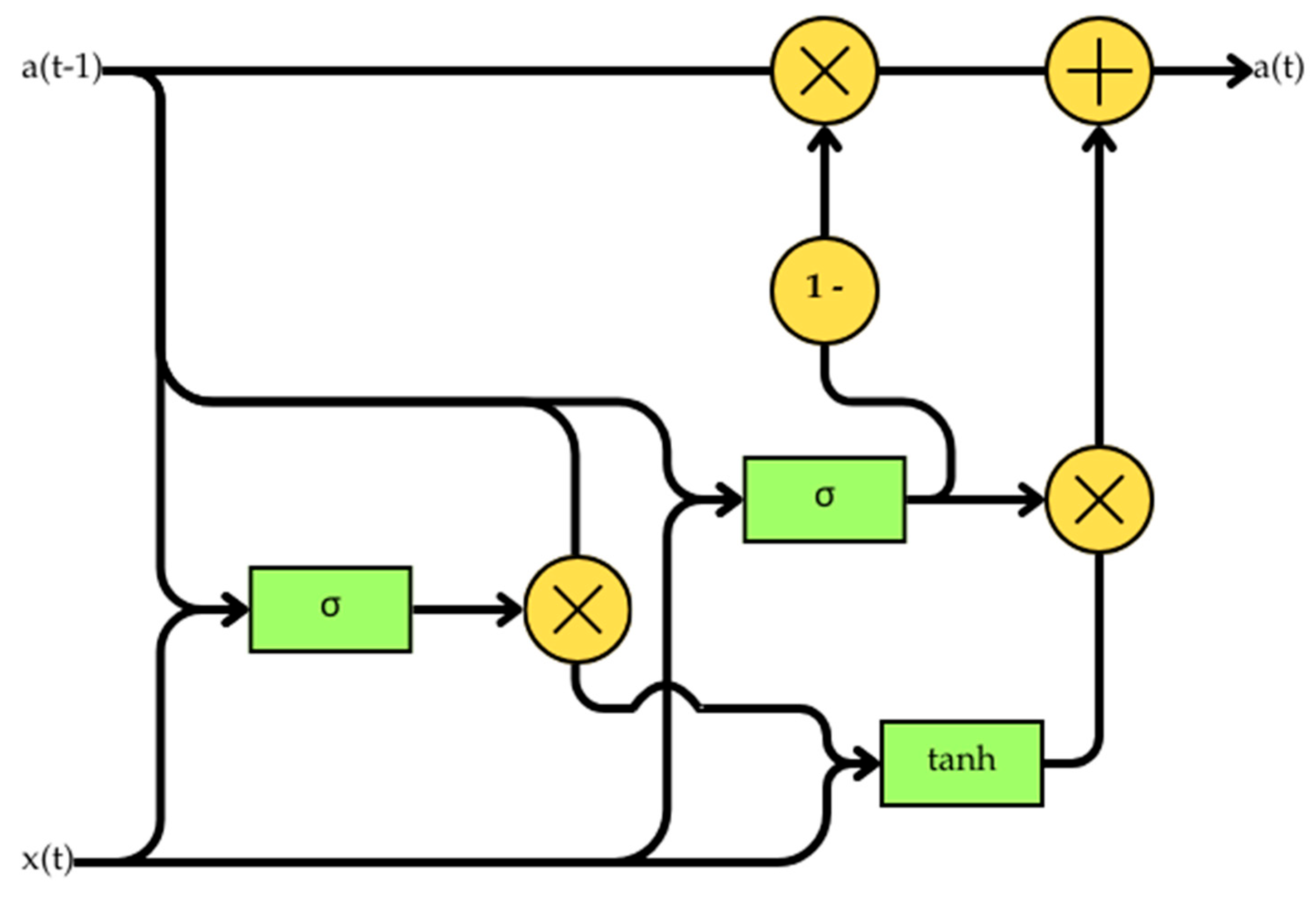
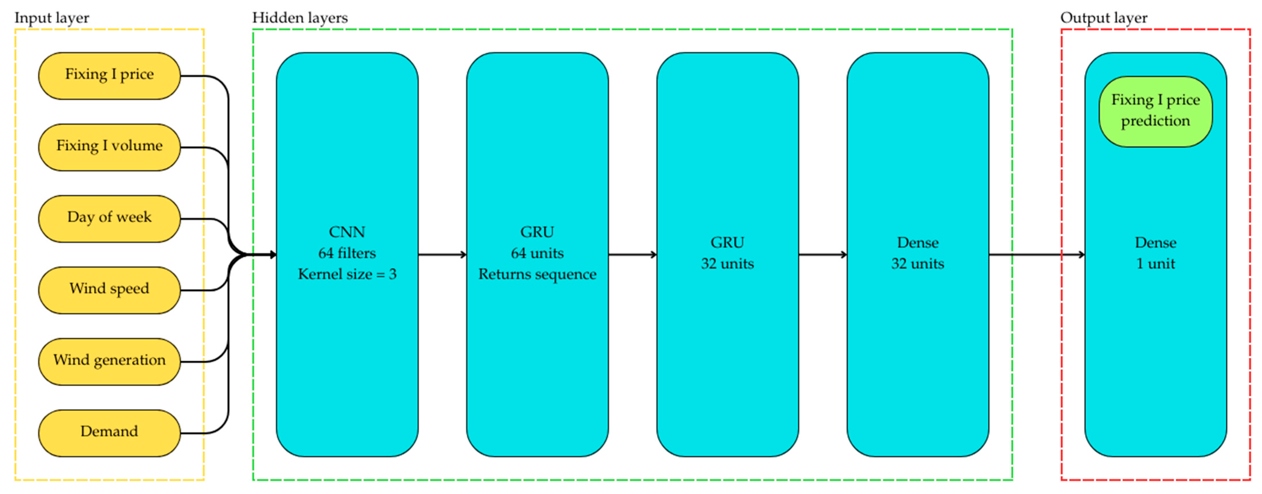
2.2. Machine Learning Models

Acquired and pre-processed data were analysed by statistical methods and functions, including regression models, which provided dependency indicators, and machine learning models, confirming these indicators as important factors of electricity prices.

While conducting research, a variety of machine learning models and their combinations were used to test the data and findings from statistical analysis, so as not to draw hasty conclusions. The research relied on artificial neural networks (ANNs), which are a branch of machine learning techniques inspired by the human nervous system. ANN consists of nodes grouped in layers, including an input layer, one or more hidden layers, and an output layer. Each node is connected to others in adjacent layers, and each connection has a weight value assigned to it. Nodes work by calculating weighted sums of their inputs and passing the results through a nonlinear activation function [36]. The simple neuron model function is shown in Equation (1) [37], where a represents the output of a single neuron, σ is a nonlinear activation function, w is the weight vector, x represents the input vector, and b denotes bias.

$$a\left(x\right)=\sigma \left(w^{T}x+b\right)$$

(1)

A feedforward neural network (FNN) is a basic type of ANN. In an FNN, data can only flow in one direction, from input nodes (neurons), through hidden layers, to output nodes [38]. This means that feedback loops are not possible. The architecture of an n-layered FNN can be represented as a result of feeding the output of the neurons from the previous layer as the input to the next layer’s nodes, as shown in Equation (2), which is an extension of Equation (1), where σ is a nonlinear activation function, W denotes the weight matrices, x represents the input vector, and b denotes the respective bias. Figure 7 presents a graphical representation of this architecture.

$$f\left(x\right)={\sigma }_n\left(W_n\cdot {\sigma }_{n-1}\left(W_{n-1}\dots {\sigma }_1\left(W_1\cdot x+b_1\right)\dots +b_{n-1}\right)+b_n\right)$$

(2)

On the contrary, the architecture of a recurrent neural network (RNN) is based on a feedback loop. Outputs can be fed to the previous layers via a hidden state containing the recurrent information, resulting in a kind of circular graph, as can be seen in Figure 8 [39]. It is worth noting that a node can be connected to itself. Because of this property, the RNNs are very useful at dealing with sequential data, but face a problem when handling long-term dependencies, as the hidden error states flowing backwards tend to either vanish or explode [40]. This problem is often referred to as the “vanishing gradient problem”. Equation (3) [40] presents a regular recurrent neuron function, where a_t represents the output of a singular neuron, σ is a nonlinear activation function, w_a and w_x denote the recurrent information and input weight vectors, x represents the input vector, and b denotes bias.

$$a_t=\sigma \left(w_a\cdot a_{t-1}+w_x\cdot x_t+b\right)$$

(3)

To combat the vanishing gradient problem, in 1997, Hochreiter and Schmidhuber proposed a new type of recurrent neuron—the long short-term memory (LSTM) cell [41]. LSTM improved RNNs by introducing input, output, and, in later versions, forget gates into the neuron, which allowed cells to remember and, unlike regular RNNs, forget values over time. The input gate assigns a value between 0 and 1 to every piece of new information, and based on that, decides what should be discarded and what should be kept. The same mechanism applies to the forget gate, although considering both the input and the recurrent state. Finally, the output gate decides, based on the current and previous states, which pieces of information should be passed on [40,41]. Figure 9 represents a single LSTM neuron with the forget gate (Figure 9a), input gate (Figure 9b) and output gate (Figure 9c), where the nonlinear function activation blocks are σ, representing the sigmoid function, and tanh, representing the hyperbolic tangent, while $\oplus$ and $\otimes$ represent pointwise addition and multiplication, respectively. The same cell can be represented mathematically as Equations (4)–(9) [40], where a_t represents the output of a neuron, σ and tanh are nonlinear activation functions, w denotes the weights, x is the input, b denotes bias, and c is the cell state.

$$f_t=\sigma \left(w_{fa}\cdot a_{t-1}+w_{fx}\cdot x_t+b_f\right)$$

(4)

$$i_t=\sigma \left(w_{ia}\cdot a_{t-1}+w_{ix}\cdot x_t+b_i\right)$$

(5)

$$\overline{c}=tanh\left(w_{\overline{c}a}\cdot a_{t-1}+w_{\overline{c}x}\cdot x_t+b_{\overline{c}}\right)$$

(6)

$$c_t=f_t\cdot c_{t-1}+i_t\cdot {\overline{c}}_t$$

(7)

$$o_t=\sigma \left(w_{oa}\cdot a_{t-1}+w_{ox}\cdot x_t+b_o\right)$$

(8)

$$h_t=o_t\cdot \mathit{tanh}\left(c_t\right)$$

(9)

To reduce the number of parameters in an LSTM model, Chu et al. (2014) introduced the RNN encoder–decoder model, which implemented a novel type of hidden unit, now commonly known as the gated recurrent unit (GRU) [42]. It optimises the architecture of an LSTM cell by reducing the number of gates to two, namely, the update gate and the reset gate. The update gate determines whether the hidden state should be updated with a new hidden state, while the reset gate decides whether the previous hidden state should be ignored or not [42,43]. Figure 10 presents a GRU neuron.

The most accurate price prediction model trained on a choice of aforementioned datasets during the study was a combined GRU and convolutional neural network (CNN) model, trained using time series cross-validation. This architecture has already been used and tested in similar time series applications, such as load or air temperature forecasting [45,46]. Its architecture is shown in Figure 11. The first layer is the convolution layer aimed at extracting local patterns. The next two layers are both GRU layers—the first, with 64 units, returns the full sequence to the second, which has 32 units. These RNN layers are designed to capture long-term dependencies and aggregate the contextual information. The last two layers serve as the additional feature combiner and the output.

The price prediction ML model compiled during the study was trained using historical electricity prices and demand, as well as wind speed and wind generation data. It allows for precise electricity price predictions for either 1 or 24 h ahead. The model outputs a time series of electricity prices, which are later plotted and compared to the subset of the test data. Other statistical methods led to the acquisition of correlation and determination coefficients, which allow for a better understanding of the relationships between electricity prices and wind speed.

3. Results and Discussion

This section presents the results obtained by employing the proposed modelling framework. The analysis focuses on key indicators such as the Pearson correlation coefficient between wind speed (or other variables) and electricity price, and the coefficient of determination derived from linear regression models. This analysis led to selecting the most appropriate input variables for the price prediction machine learning models. These models were used to assess the impact of the selected input variables as important to the electricity price. The accuracy of these models, and by extension, the level of impact of selected input variables, was measured using the mean absolute error (MAE).

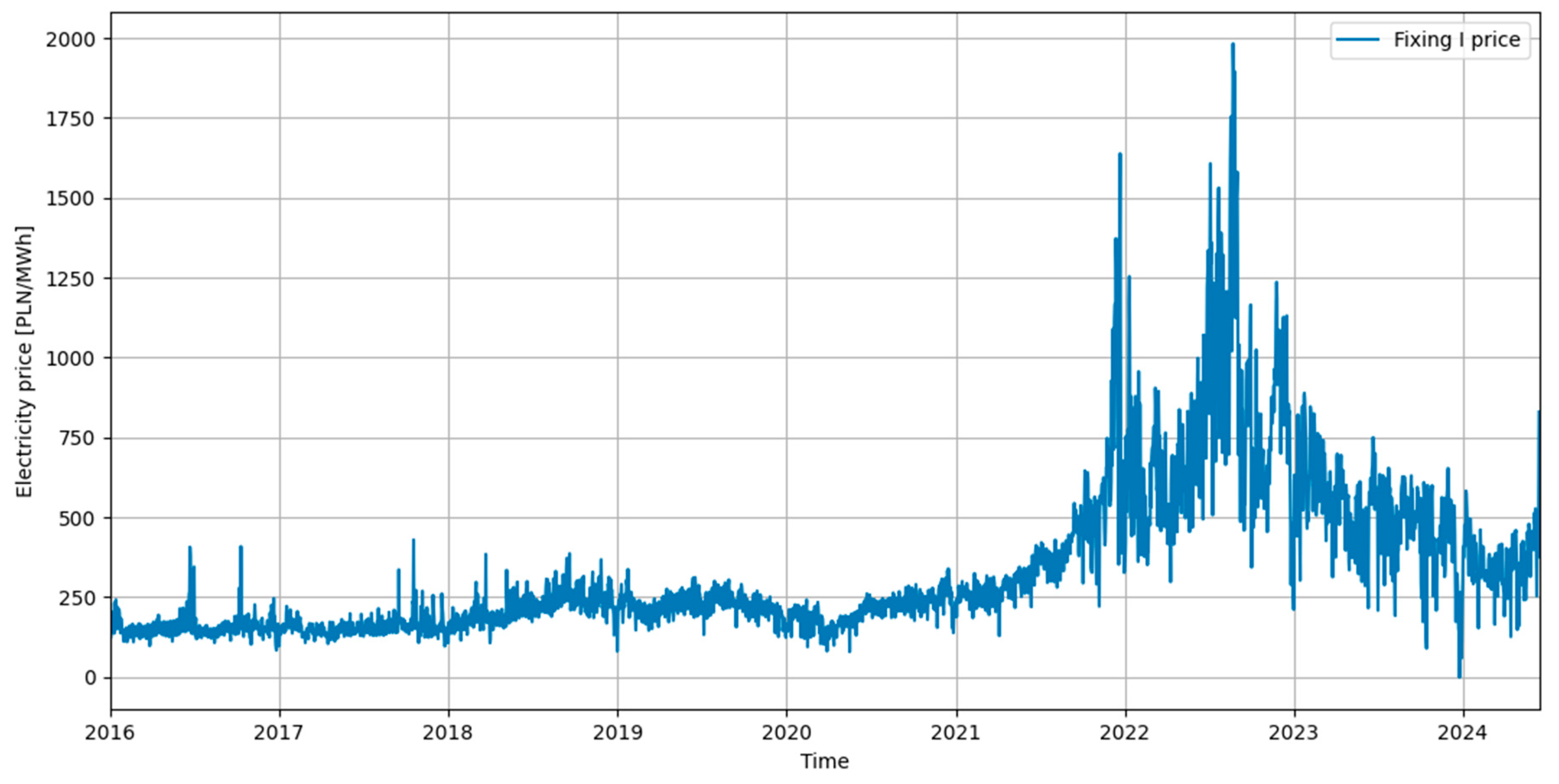
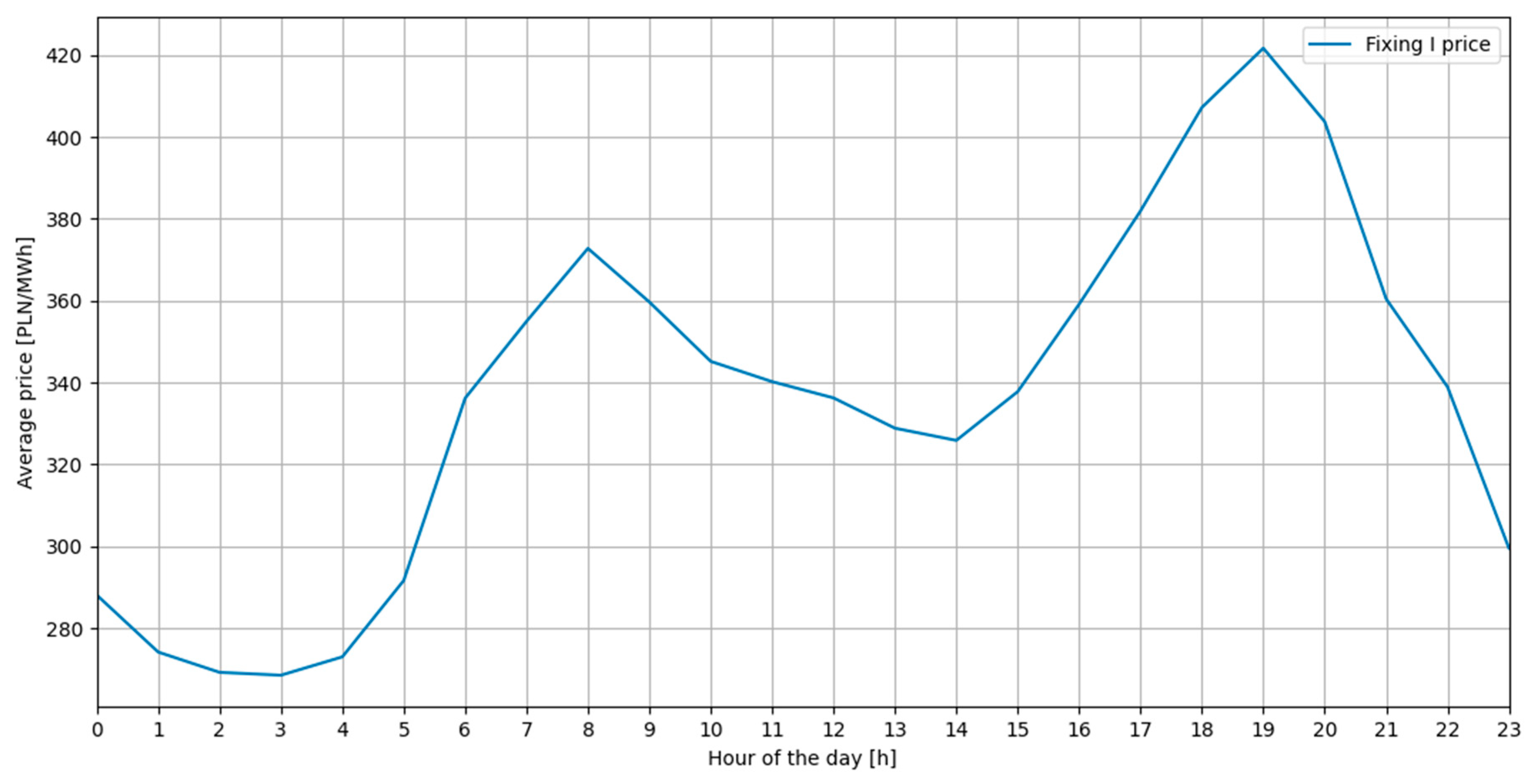
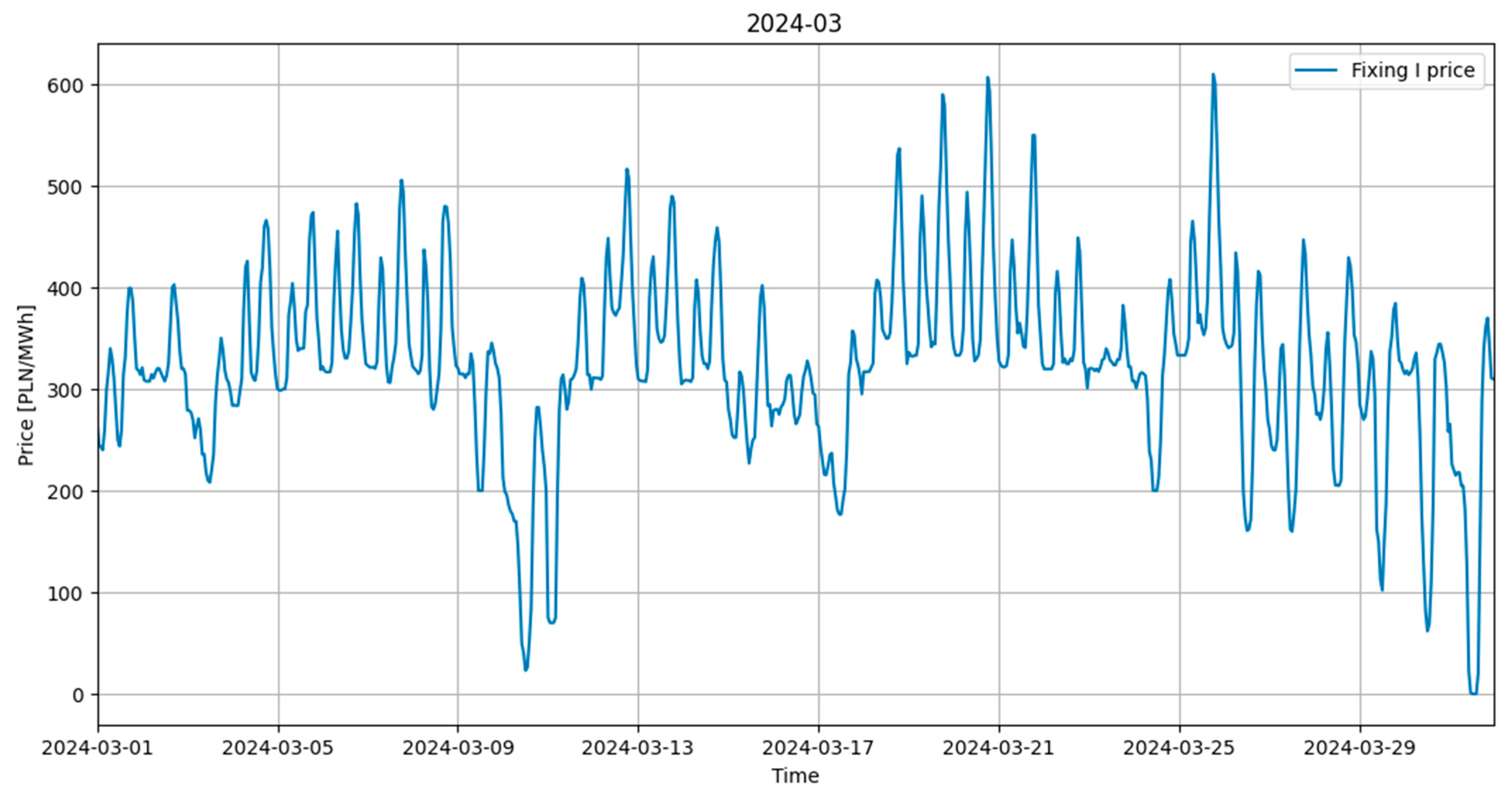
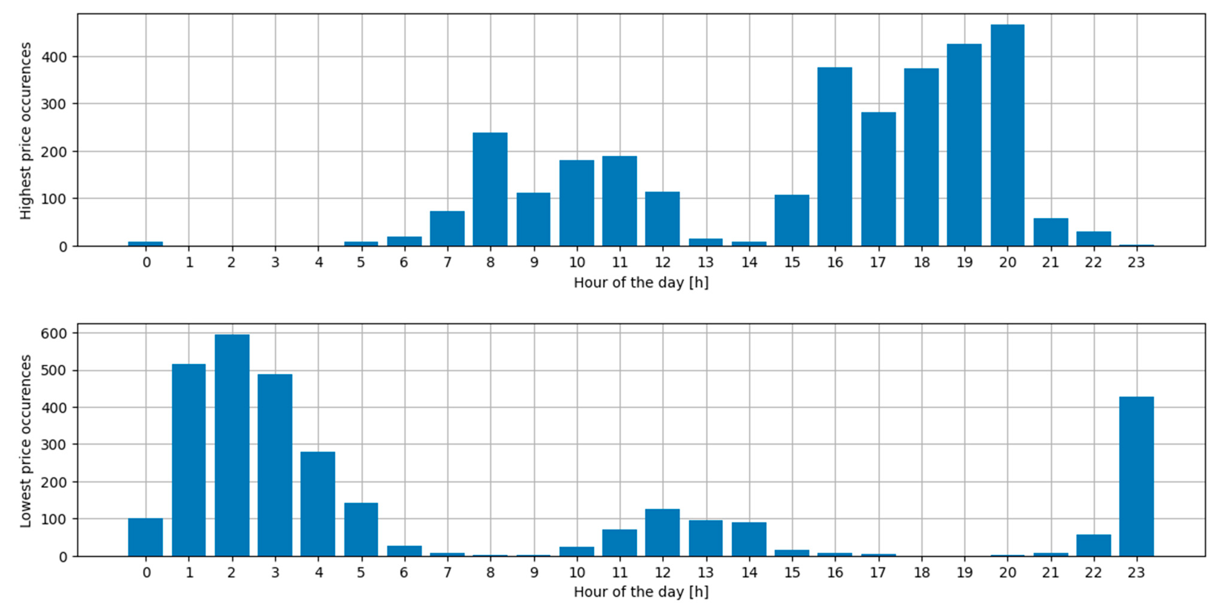
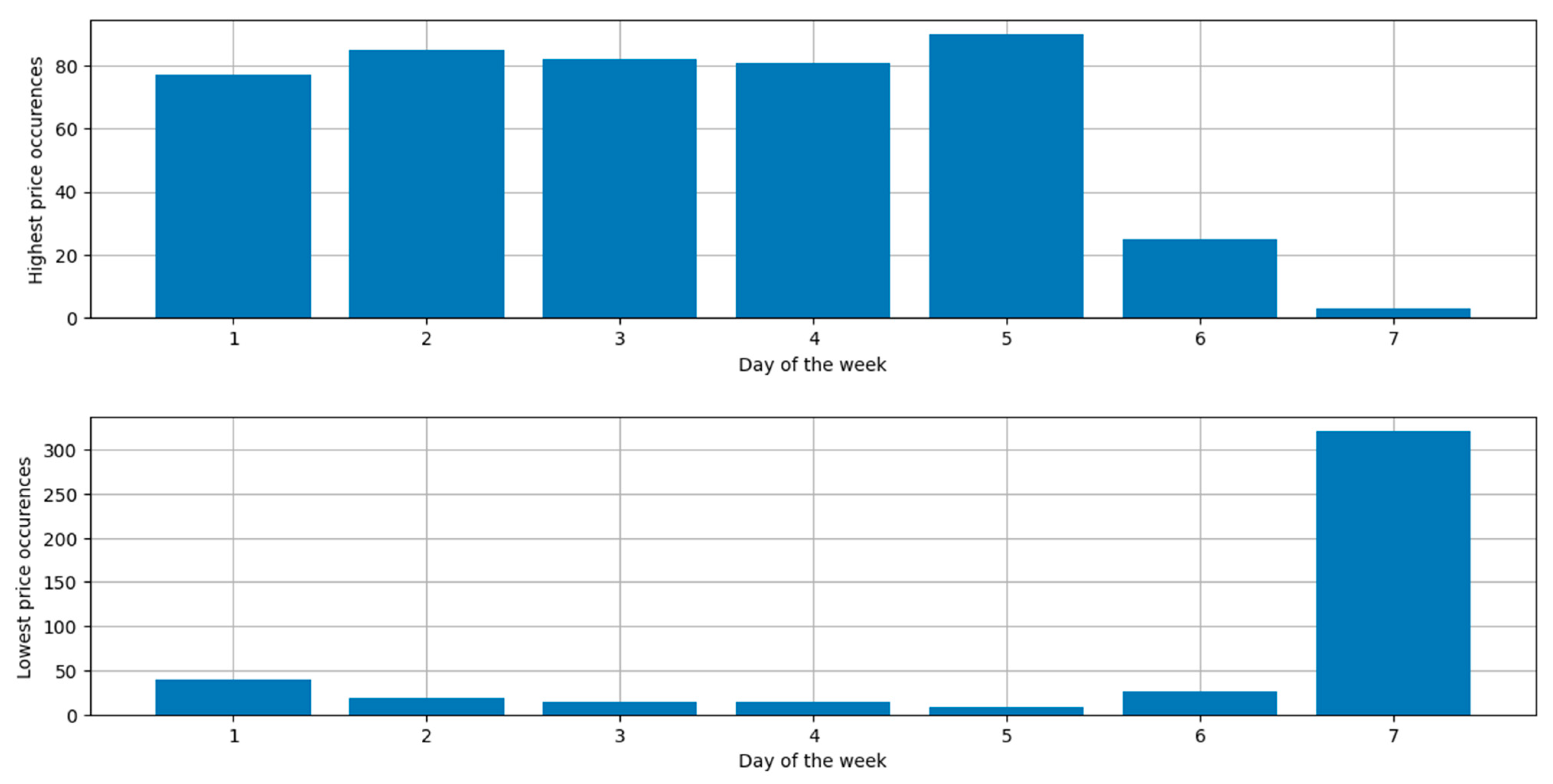
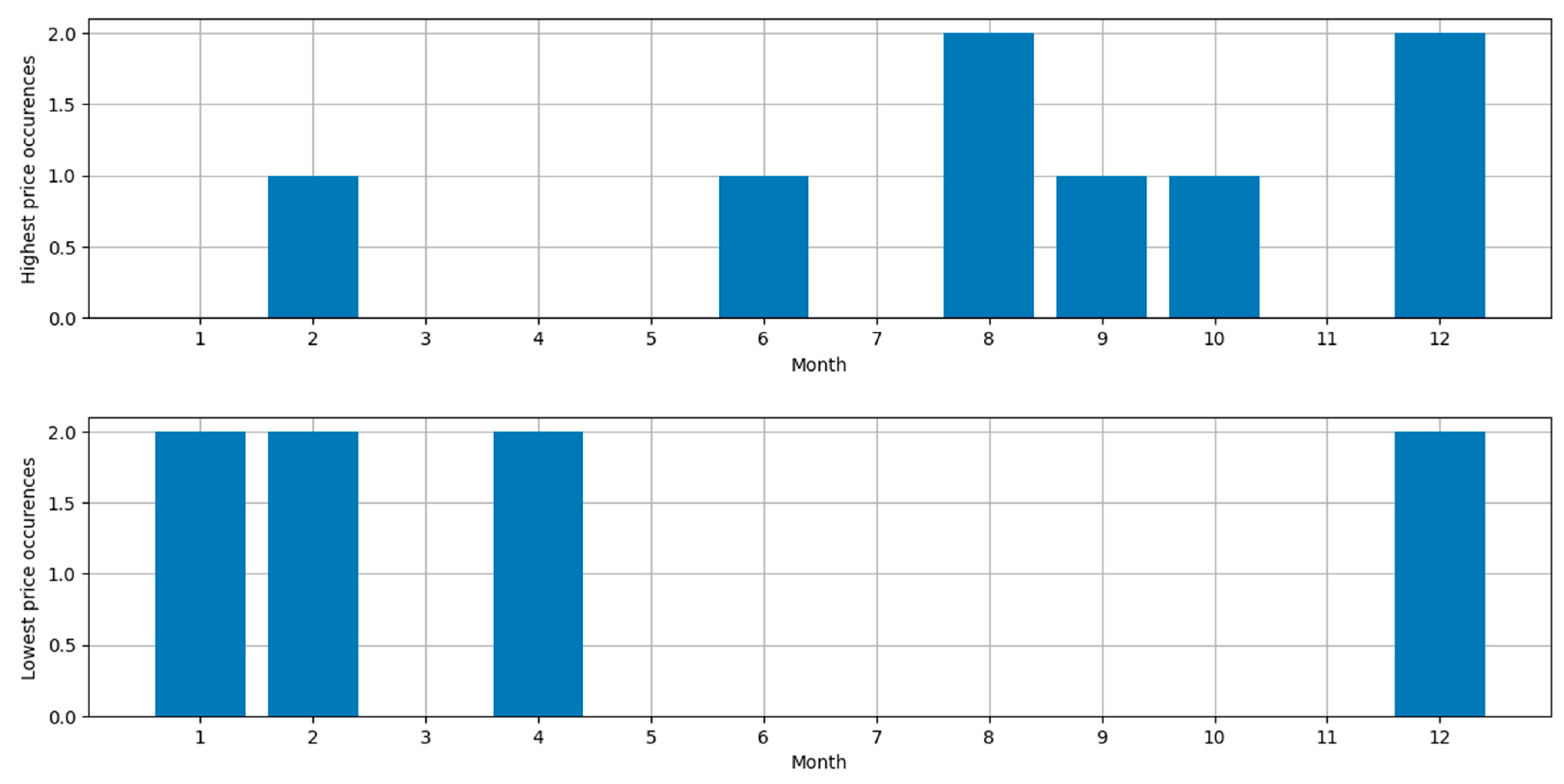
3.1. Price Data Analysis

The analysed historical data were collected on an hourly basis. The initial visual analysis revealed a cyclical nature of the data. This temporal dependence was subsequently examined in more detail by dividing the dataset into daily, weekly, and monthly subsets. These were then reanalysed visually to learn more about temporal cycles affecting price variations.

The analysis of the results, supported by graphical examination of the plotted data points, enabled the formulation of several key conclusions on the Polish energy market. Firstly, the electricity price varies over the course of a day. Each day shows an easily recognisable pattern, as shown in Figure 12, that repeats over time. This pattern is also evident on a larger scale in Figure 13, as it is present every day of every month, regardless of the overall trend or price level. The daily pattern consists of two peaks connected by periods of lowered prices. By calculating the average price for every hour of the day, the average position of the daily peaks becomes clearer, as can be seen in Figure 12. These daily peaks tend to occur around 8 a.m. and 7 p.m., which is related to the diurnal activity patterns of consumers [47]. Unsurprisingly, the distribution outline of both the highest and lowest daily electricity prices from 3086 days, as shown in Figure 14, closely follows the average price plot. Most commonly, the highest prices occur in the evenings, around 8 p.m., while the lowest prices occur during the night, around 2 a.m. As can already be seen, electricity prices are highly temporal on a daily scale. This temporality prompted the use of a recurrent neural network as the prediction model.

Extending the analysis to a broader, weekly scale leads to another conclusion. When considering the average electricity price per day of the week, it is evident that, on average, prices are lowest on Sundays and highest on Tuesdays and Wednesdays, as shown in

Table 1. Average electricity price per day of the week.

Day of Week	Average Price [PLN/MWh]
Monday	347.56
Tuesday	361.53
Wednesday	361.45
Thursday	352.58
Friday	348.13
Saturday	319.39
Sunday	264.30

, as well as in Figure 13, where a significant drop in price can be observed every Sunday. Figure 15, which shows the distribution of the highest and lowest daily average prices per day of week, from 441 weeks, further supports that weekly pattern. Furthermore, it is far less feasible to single out a day of the week when the highest electricity prices occur most often, as those are distributed fairly evenly between Monday and Friday, while it is clear that Sunday is the most likely day of the lowest average price.

Again, applying a larger scale to the same line of thinking reveals yet another seasonal pattern. As can be seen in

Table 2. Average electricity price per month.

Month	Average Price [PLN/MWh]
January	319.09
February	295.00
March	299.93
April	292.43
May	303.79
June	354.04
July	371.00
August	402.27
September	364.10
October	328.74
November	354.96
December	368.99

, the average electricity prices tend to be lowest in the winter and early spring, and highest during the summer and late autumn. This is again supported by the highest and the lowest average monthly price distribution shown in Figure 16. It was due to these temporal patterns, that additional, artificial variables were added to the dataset: year, month, week of the year, day of the week, day of the month, and hour of the day, derived from the date, as well as the information if it’s weekend and if it’s a day of peak weekly demand (“peak day”—taking 1 for Mondays—Fridays, 0 for Saturdays and −1 for Sundays). These variables were supposed to enhance and clarify time dependencies for the machine learning model.

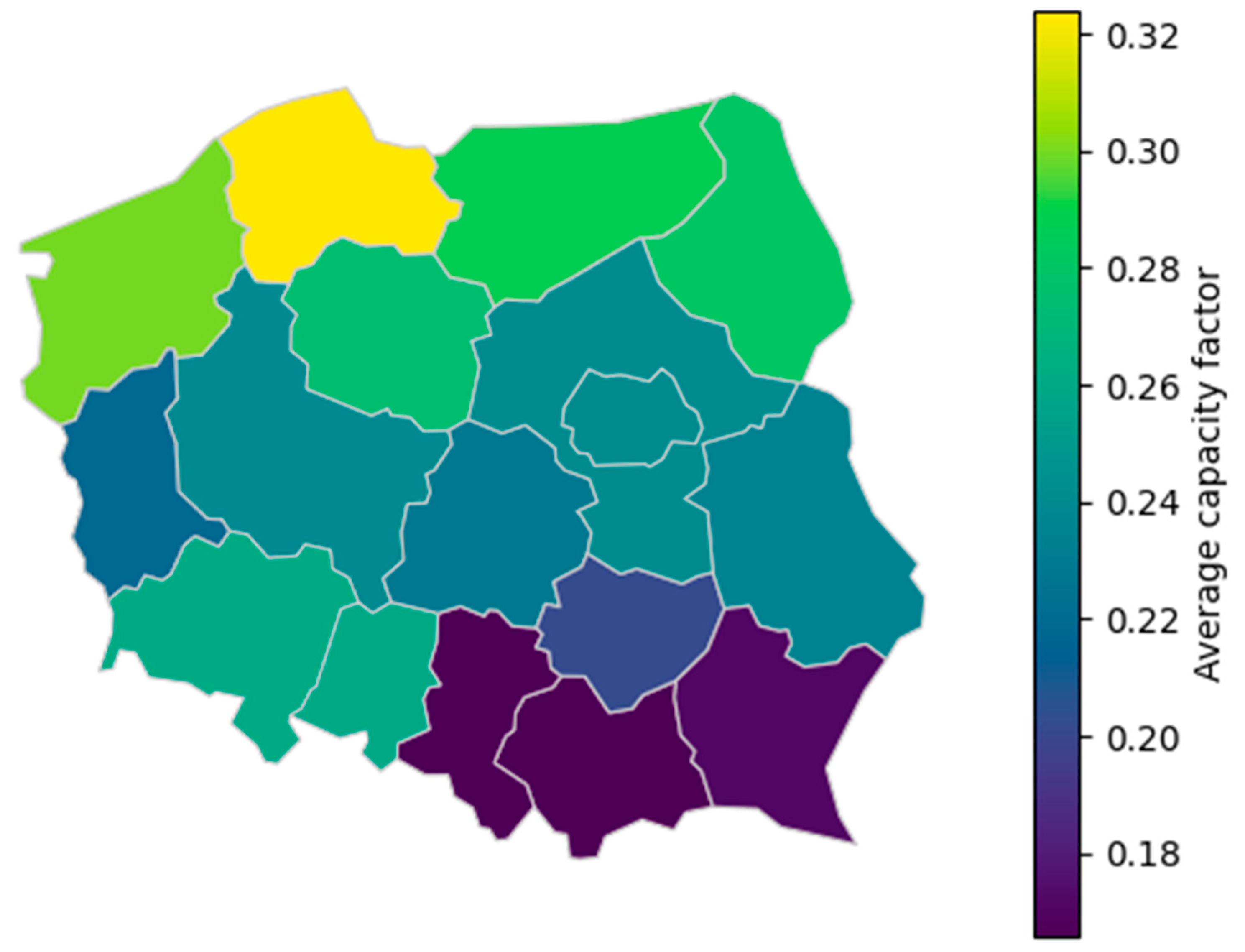
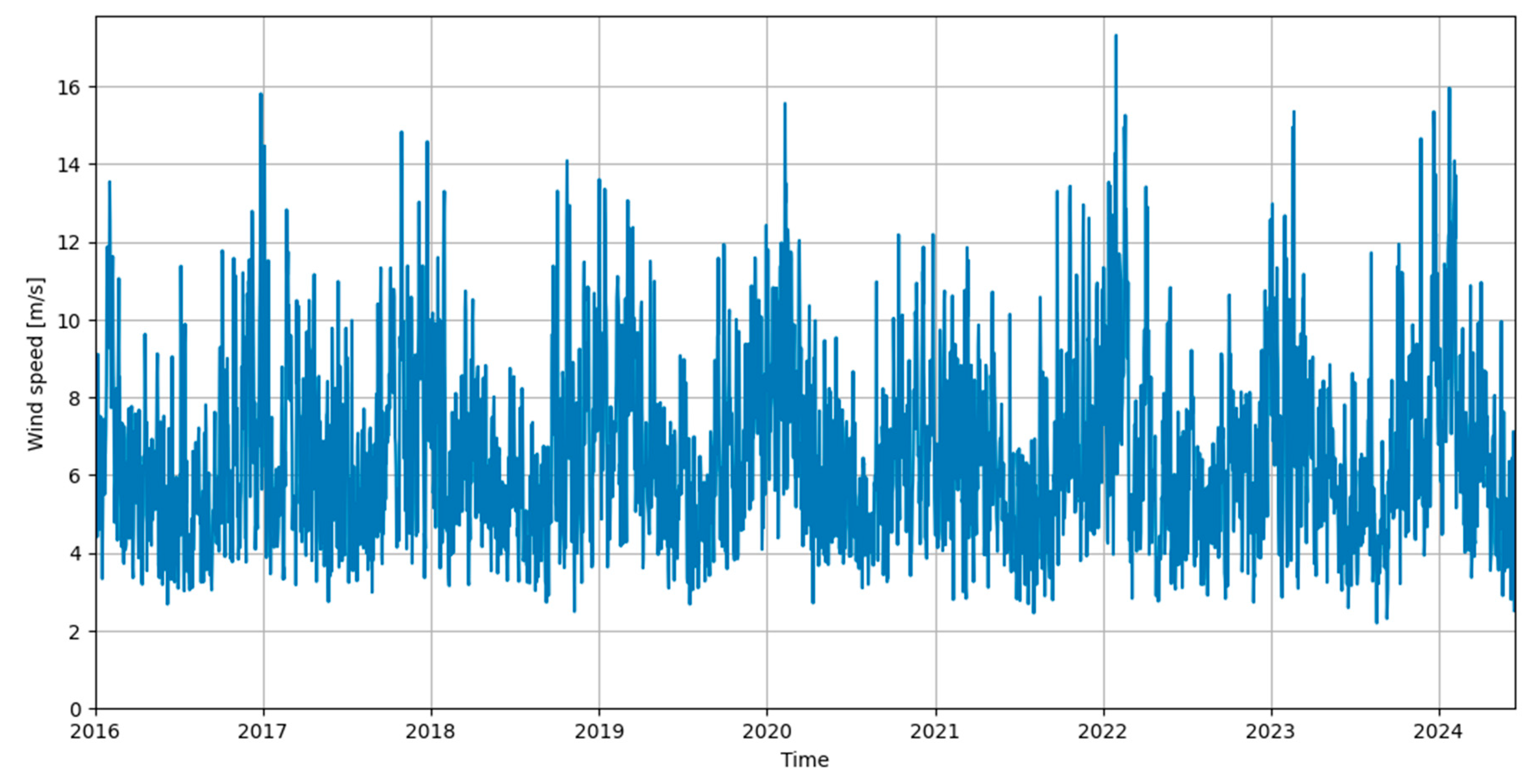
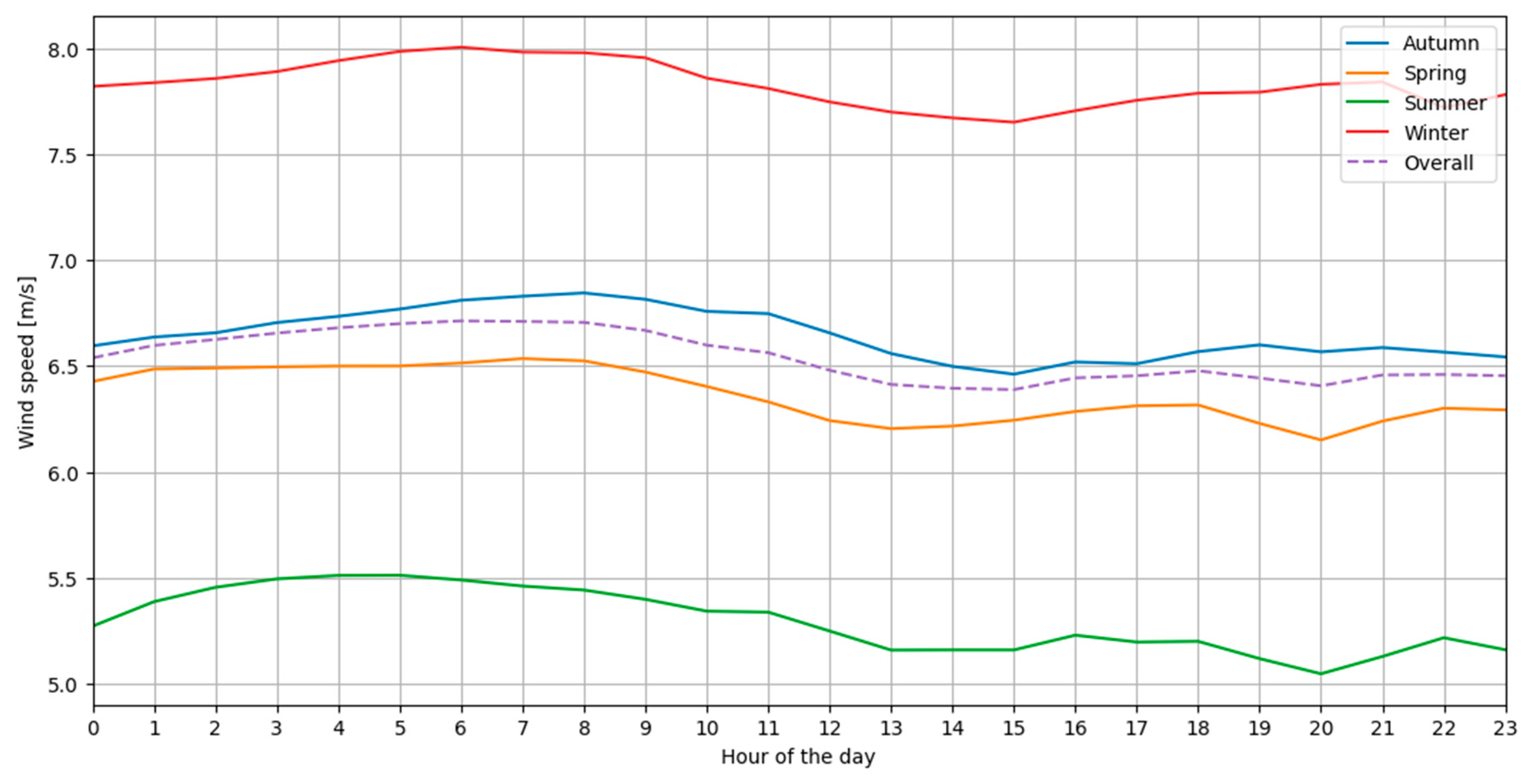
3.2. Wind Speed Data Analysis

In order to analyse the hourly wind speed data, which came from ERA5 reanalysis, it was necessary to compare them to some real-life measurements to assess their bias and accuracy. This was achieved by comparing daily average wind speed data, extrapolated to 100 m, from a weather station in Kołobrzeg-Dźwirzyno, Poland, to its corresponding data points from ERA5. Wind speed data were extrapolated using the Hellman exponential law, as explained by Banuelos-Ruedas et al. (2010) [48], and shown in Equation (10) [39], where $v$ is the wind speed, $h$ is the height, and $\alpha$ is the friction coefficient, depending on the type of landscape. In this comparison, an α coefficient equal to 0.25 was chosen, as the considered weather station lies near the coast, but close to trees [48]. The closest ERA5 datapoint was located some 8 km southeast of the weather station. The average absolute difference between the extrapolated wind speeds and the reanalysis from ERA5 reached 0.81 m/s, corresponding to a 12.99% relative error. This error could also be, at least partially, caused by the spatial difference between the two locations.

$$v=v_0\cdot {\left({\displaystyle \frac{h}{h_0}}\right)}^{\alpha }$$

(10)

Analysing wind speed over time (see Figure 17) shows that the average daily wind speed also exhibits temporal variability. Higher wind speeds tend to occur during winter months, as presented in

Table 3. Average wind speed per month and season at a height of 100 m.

Month	Average Wind Speed [m/s]	Season	Average Wind Speed [m/s]
December	7.85	Winter	7.83
January	7.79
February	7.85
March	6.69	Spring	6.36
April	6.51
May	5.90
June	5.29	Summer	5.30
July	5.42
August	5.18
September	5.87	Autumn	6.65
October	7.18
November	6.87

and Figure 18, while during summer months, wind speeds tend to be lower. The difference between average wind speeds between December and February and August is 2.67 m/s. December turned out to be the most likely month of the highest average wind speed, while June and August were identified as the most likely months with the lowest average wind speed.

This seasonal trend becomes even more evident when considering average hourly wind speeds. As illustrated in Figure 19, the overall pattern of daily wind speed variation remains consistent for different seasons, although their amplitudes vary. It is worth noting that, while wind speed is highly variable and therefore difficult to predict, the average wind speed per hour of the day remains relatively stable. The biggest difference between maximum and minimum hourly wind speed is 0.46 m/s and occurs during an average summer. Wind speed tends to reach its highest values between 4 a.m. and 9 a.m. and its lowest values between 2 p.m. and 8 p.m.

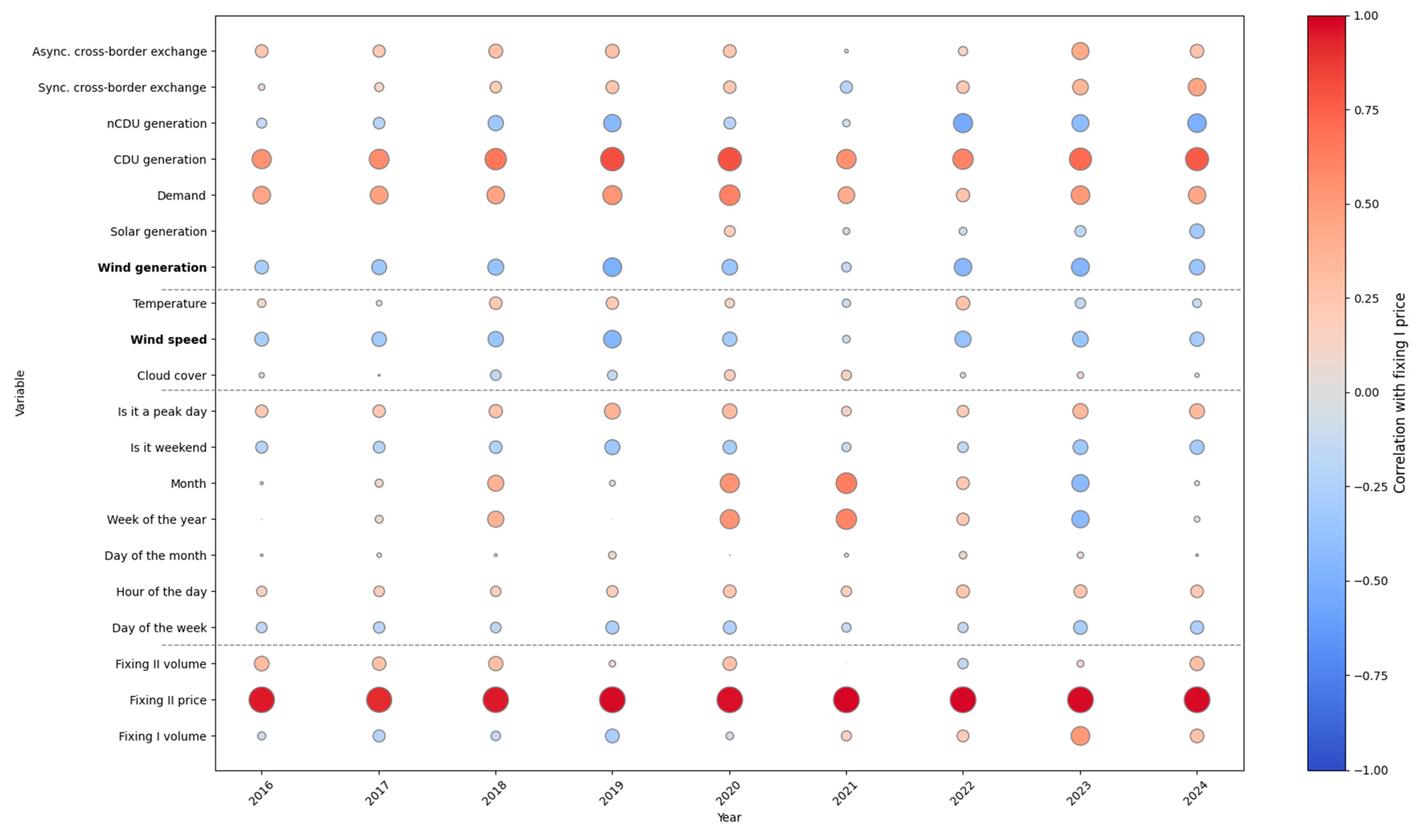
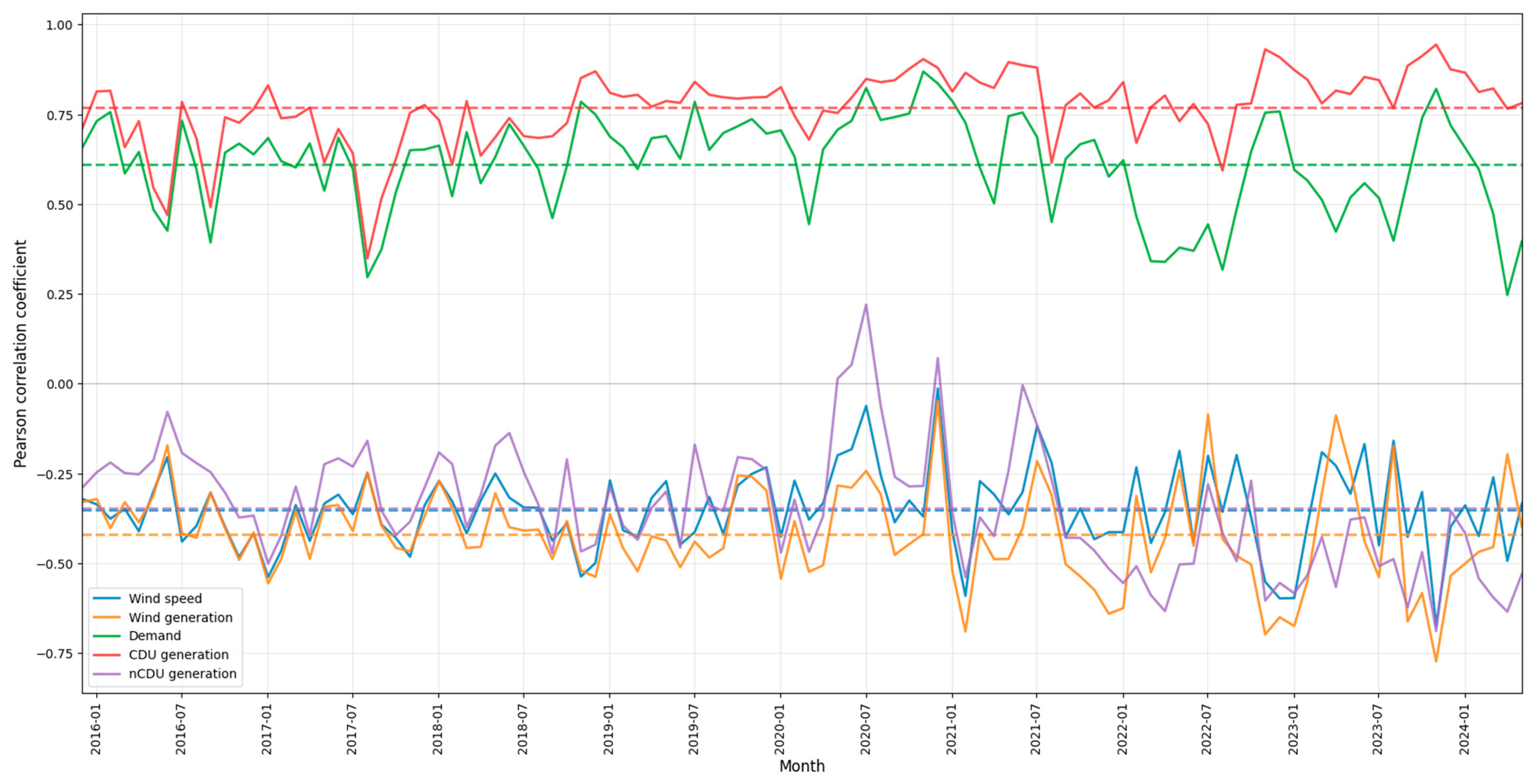
3.3. Statistical Analysis Results

Initial statistical analysis showed that the Pearson correlation coefficients rarely exceeded |0.1|, the highest being that of a year (0.57), centrally dispatched units (CDU) generation (0.31), and demand (0.24). Wind speed correlation coefficient reached −0.17. Low p-values (less than 0.05) suggest that these correlations are statistically significant; however, linear regression models exhibited large condition numbers, suggesting high multicollinearity. This fact may undermine the statistical significance of those relations, as the effects of individual variables are not clear. Using the generalised least squares (GLS) linear regression model showed that the adjusted R² is again the highest for the year variable, explaining c. 31.80% of the variance, while the wind speed only explained about 2.86% of the variance.

A naïve approach to the statistical analysis yields varying results. By analysing the time series, it has been determined that the most important factor impacting the electricity price is time, suggesting a high seasonal or other temporal dependency. Because of that, the statistical analysis was repeated over smaller time windows (years, seasons, months, and days) in order to better understand other factors. New results, shown in

Table 4. Pearson correlation coefficient and R² coefficient for the relationship between the chosen variables and electricity price.

Year		2016	2017	2018	2019	2020	2021	2022	2023	2024
Correlation coefficient	CDU generation	0.539	0.567	0.664	0.806	0.796	0.549	0.603	0.714	0.773
	Demand	0.452	0.467	0.452	0.530	0.612	0.408	0.259	0.507	0.442
	Wind generation	−0.274	−0.329	−0.374	−0.503	−0.357	−0.136	−0.450	−0.466	−0.353
	Wind speed	−0.287	−0.312	−0.345	−0.454	−0.299	−0.085	−0.383	−0.359	−0.302
R2	CDU generation	0.290	0.321	0.441	0.649	0.633	0.301	0.363	0.509	0.597
	Demand	0.204	0.218	0.205	0.281	0.374	0.166	0.067	0.257	0.195
	Wind generation	0.075	0.108	0.139	0.253	0.127	0.018	0.202	0.217	0.124
	Wind speed	0.082	0.097	0.119	0.206	0.089	0.007	0.146	0.128	0.091

, suggest that, generally speaking, the CDU generation, demand, and wind generation (wind speed) are the most influential factors. The only exception to that was the year 2021, when again the time variables had the biggest impact on the price. On a yearly basis, the CDU generation has the highest impact on electricity prices, showing both the highest correlation coefficient (no less than 0.539) and the highest R² (no less than 0.29). The CDU generation was followed closely by the demand, which for every year achieved a correlation coefficient higher than 0.298, and R² higher than 0.2. Wind generation and wind speed, while not identical, seem to be highly related. The difference between them may have been caused by the reanalysis error, as the wind generation derives from the wind speed to a large degree. All calculated correlation coefficients per year are presented in Figure 20.

The results presented in Figure 20 and Table 4 suggest that the electricity price is strongly related to the energy mix. General statistics are included in

Table A1. Overall analysis.

Variable	ρS	p (ρS)	ρP	p (ρP)	R2	F-Stat	p (F-Stat)	t-Test β0	β0 Std. Error	Est. Slope Coef. β	β Std. Error	Omnibus	p (Omnibus)	DW	JB	p (JB)	Condition Number	VIF
Fixing I price	1.00	0.00	1.00	0.00	1.00	4.57 × 1033	0.00	0.00	0.00	1.00	0.00	49,286.07	0.00	0.05	844,942.80	0.00	691.15
Fixing I volume	0.43	0.00	0.39	0.00	0.15	13,348.42	0.00	57.75	2.58	0.11	0.00	51,005.41	0.00	0.07	1,075,659.57	0.00	7477.47	2.00
Fixing II price	0.99	0.00	0.99	0.00	0.98	3,547,233.37	0.00	−0.02	0.23	1.01	0.00	39,201.50	0.00	0.53	6,249,838.06	0.00	689.36	2.00
Fixing II volume	0.16	0.00	0.05	0.00	0.00	216.42	0.00	308.33	2.15	0.03	0.00	49,276.42	0.00	0.05	827,143.04	0.00	2108.79	1.19
Day of the week	−0.12	0.00	−0.09	0.00	0.01	646.98	0.00	373.64	1.76	−12.40	0.49	48,588.08	0.00	0.05	801,105.55	0.00	6.85	2.83
Hour of the day	0.11	0.00	0.11	0.00	0.01	854.79	0.00	289.12	1.89	4.11	0.14	47,921.91	0.00	0.05	760,041.72	0.00	26.14	1.72
Day of the month	0.02	0.00	0.02	0.00	0.00	45.03	0.00	324.71	2.00	0.75	0.11	48,500.01	0.00	0.05	790,773.86	0.00	36.86	1.10
Week of the year	0.07	0.00	0.08	0.00	0.01	532.20	0.00	297.88	1.94	1.49	0.06	48,128.84	0.00	0.05	778,396.53	0.00	59.35	21.80
Month	0.08	0.00	0.09	0.00	0.01	595.07	0.00	292.70	2.04	6.89	0.28	48,126.98	0.00	0.05	779,512.89	0.00	15.34	21.43
Year	0.75	0.00	0.56	0.00	0.32	34,536.17	0.00	−12,3668.68	667.27	61.40	0.33	58,391.44	0.00	0.07	2,052,659.13	0.00	1,666,030.32	2.40
Is it weekend	−0.15	0.00	−0.11	0.00	0.01	837.33	0.00	354.25	1.15	−62.40	2.16	48,652.26	0.00	0.05	803,981.14	0.00	2.44	8.18
Is it peak day	0.16	0.00	0.12	0.00	0.01	1057.01	0.00	311.61	1.24	43.42	1.34	48,647.01	0.00	0.05	805,297.41	0.00	2.07	8.61
Cloud cover	0.01	0.00	0.02	0.00	0.00	21.03	0.00	322.15	3.26	2.64	0.58	48,646.22	0.00	0.05	801,694.46	0.00	19.45	1.35
Wind speed	−0.19	0.00	−0.17	0.00	0.03	2179.17	0.00	452.82	2.67	−17.79	0.38	47,892.31	0.00	0.05	769,489.85	0.00	19.78	2.42
Temperature	0.06	0.00	0.04	0.00	0.00	141.84	0.00	−82.77	35.21	1.48	0.12	48,300.53	0.00	0.05	773,990.08	0.00	10,188.52	5.39
Wind generation	−0.06	0.00	−0.06	0.00	0.00	278.10	0.00	355.81	1.52	−0.01	0.00	48,114.13	0.00	0.05	772,899.72	0.00	3726.30	22.26
Solar generation	0.10	0.00	−0.01	0.07	0.00	3.22	0.07	485.80	1.85	0.00	0.00	19,965.39	0.00	0.06	215,931.74	0.00	2328.50	15.07
Demand	0.32	0.00	0.24	0.00	0.06	4683.92	0.00	−54.66	5.79	0.02	0.00	48,754.70	0.00	0.05	836,456.60	0.00	119,131.21	201.54
CDU generation	0.31	0.00	0.31	0.00	0.10	7955.73	0.00	−7.78	3.97	0.03	0.00	45,319.59	0.00	0.05	685,916.43	0.00	54,040.35	209.28
nCDU generation	0.03	0.00	−0.02	0.00	0.00	36.27	0.00	353.43	2.99	0.00	0.00	48,310.74	0.00	0.04	780,558.39	0.00	21,223.05	157.14
Sync. cross-border exchange	−0.08	0.00	−0.14	0.00	0.02	1554.91	0.00	333.73	0.97	−0.04	0.00	48,267.29	0.00	0.05	800,504.24	0.00	885.53	27.55
Async. cross-border exchange	0.08	0.00	0.05	0.00	0.00	152.76	0.00	323.36	1.44	0.02	0.00	48,505.60	0.00	0.05	786,934.18	0.00	1154.56	7.66
Season	0.02	0.00	0.03	0.00	0.00	55.63	0.00	326.96	1.60	6.42	0.86	48,617.93	0.00	0.05	801,382.42	0.00	3.66	1.72

, while yearly statistics from 2016 in

Table A2. Yearly analysis (2016).

Variable	ρS	p (ρS)	ρP	p (ρP)	R2	F-Stat	p (F-Stat)	t-Test β0	β0 Std. Error	Est. Slope Coef. β	β Std. Error	Omnibus	p (Omnibus)	DW	JB	p (JB)	Condition Number
Fixing I price	1.00	0.00	1.00	0.00	1.00	3.91 × 1032	0.00	0.00	0.00	1.00	0.00	7727.33	0.00	0.00	483,342.70	0.00	443.72
Fixing I volume	−0.16	0.00	−0.09	0.00	0.01	79.51	0.00	185.86	2.98	−0.01	0.00	9763.96	0.00	0.20	1,026,091.70	0.00	8497.05
Fixing II price	0.96	0.00	0.95	0.00	0.91	86781.17	0.00	−2.47	0.59	1.03	0.00	5819.44	0.00	0.76	3,599,945.29	0.00	458.96
Fixing II volume	0.51	0.00	0.31	0.00	0.10	962.97	0.00	123.19	1.38	0.06	0.00	10,153.28	0.00	0.22	1,247,658.80	0.00	1352.76
Day of the week	−0.22	0.00	−0.17	0.00	0.03	253.89	0.00	177.31	1.30	−5.73	0.36	9747.71	0.00	0.20	1,059,040.61	0.00	6.88
Hour of the day	0.29	0.00	0.15	0.00	0.02	209.09	0.00	142.79	1.40	1.50	0.10	9881.35	0.00	0.21	1,096,864.57	0.00	26.14
Day of the month	−0.01	0.17	0.01	0.35	0.00	0.89	0.35	158.86	1.49	0.08	0.08	9670.02	0.00	0.19	1,001,926.92	0.00	37.08
Week of the year	0.00	0.84	0.00	0.99	0.00	0.00	0.99	160.10	1.48	0.00	0.05	9674.41	0.00	0.19	1,003,423.58	0.00	62.18
Month	0.02	0.11	0.01	0.24	0.00	1.39	0.24	158.46	1.56	0.25	0.21	9672.34	0.00	0.19	1,002,620.88	0.00	15.98
Is it weekend	−0.29	0.00	−0.21	0.00	0.04	411.79	0.00	169.25	0.84	−31.94	1.57	9792.63	0.00	0.21	1,084,337.57	0.00	2.43
Is it peak day	0.30	0.00	0.22	0.00	0.05	462.37	0.00	148.10	0.90	20.99	0.98	9836.19	0.00	0.21	1,109,319.00	0.00	2.07
Cloud cover	−0.01	0.17	−0.04	0.00	0.00	14.78	0.00	169.15	2.47	−1.66	0.43	9651.19	0.00	0.19	991,009.99	0.00	19.86
Wind speed	−0.34	0.00	−0.29	0.00	0.08	788.11	0.00	209.41	1.89	−7.91	0.28	9790.26	0.00	0.21	1,084,228.96	0.00	18.52
Temperature	0.07	0.00	0.11	0.00	0.01	99.45	0.00	−97.24	25.81	0.91	0.09	9575.37	0.00	0.19	955,114.49	0.00	10,079.54
Wind generation	−0.35	0.00	−0.27	0.00	0.07	711.79	0.00	182.14	1.08	−0.02	0.00	9834.60	0.00	0.21	1,103,122.05	0.00	2690.18
Demand	0.68	0.00	0.45	0.00	0.20	2249.93	0.00	−27.83	4.01	0.01	0.00	10,914.09	0.00	0.24	1,813,384.70	0.00	117,142.65
CDU generation	0.76	0.00	0.54	0.00	0.29	3590.07	0.00	−11.40	2.93	0.01	0.00	11,241.77	0.00	0.27	2,150,552.20	0.00	61,994.77
nCDU generation	−0.10	0.00	−0.15	0.00	0.02	189.79	0.00	191.64	2.40	−0.01	0.00	9607.73	0.00	0.20	976,783.51	0.00	20,481.84
Sync. cross-border exchange	−0.03	0.00	0.06	0.00	0.00	33.76	0.00	162.76	0.86	0.01	0.00	9611.64	0.00	0.20	979,482.07	0.00	547.65
Async. cross-border exchange	0.35	0.00	0.24	0.00	0.06	533.50	0.00	144.83	0.97	0.03	0.00	9927.12	0.00	0.21	1,116,873.11	0.00	942.58

, in Appendix A. As the CDUs are still responsible for the largest share of the energy mix, the price is highly correlated with the CDU generation. As PV generation gains purchase, its negative impact on prices seems to be rising. This cannot be said for other RES, as the correlations fluctuate. High temporal dependencies in 2021, alongside lower correlation coefficients with other variables, suggest that some external factors were responsible for the rising price. Demand is another highly correlated variable, which is understandable, as higher demand leads to increased production and, in turn, higher operational costs. Otherwise, temporal correlations seem to confirm earlier findings, showing that weekends are correlated with lower prices.

Figure 21 presents monthly correlation coefficients between fixing the I price and selected analysed variables. The dash-dotted lines represent averages for each of the variables. Non-centrally dispatched unit (nCDU) generation is included, as it was deemed significant to the price of electricity. As a large part of the nCDU is, in fact, composed of combined heat and power (CHP) plants, their variable price is low enough to place them at the low end of the merit order, which in turn leads to lower prices as the nCDU generation rises [49]. Due to the sheer amount of nCDU in the Polish energy mix, it is an important factor in the electricity price. This is especially evident when considering the seasonality of CHP generation, as the need for heat in colder months leads to additional electricity generation, while the lack of it in warmer seasons removes that factor. The results of the analysis indicate that wind speed and wind generation correlate with the electricity price more strongly than nCDU generation.

3.4. Prediction Results

By passing different combinations of the most relevant variables, as found in the statistical analysis, several price prediction machine learning models have been developed. Input data was rescaled using the min–max normalisation, as shown in Equation (11), where x’_i is a normalised datapoint, x_i is the input datapoint, and x_min, x_max are the minimum and maximum points in the dataset, respectively. Data used as ML models’ input was rescaled to a range between 0 and 1. Training a neural network consists of minimising the loss function—in this case, the mean squared error (MSE), presented in Equation (12), where n is the number of samples, y is the prediction, and x is the actual value, was chosen. The most accurate of the models—the GRU + CNN model with the Fixing I price and volume, day of the week, wind speed, wind generation, and demand as inputs—led to highly accurate predictions, with an MAE of around 0.006 for t + 1 h prediction, as can be seen in Figure 22. MAE is a measurement of the accuracy expressed by Equation (13), where n is the number of samples, y is the prediction, and x is the actual value. Because of the normalisation, MAE divided by 100 represents a percentage of the maximum range of values in the dataset. The same model, adjusted for t + 24 h predictions, reached an average of 0.016 MAE during evaluation.

$${x^{’}}_i={\displaystyle \frac{x_i-x_{min}}{x_{max}-x_{min}}}$$

(11)

$$MSE={\displaystyle \frac{{\sum }_{i=1}^n{\left(x_i-y_i\right)}^2}{n}}$$

(12)

$$MAE={\displaystyle \frac{\sum _{i=1}^n\left|x_i-y_i\right|}{n}}$$

(13)

This model, while pretty accurate overall, was not able to predict peaks with acceptable precision. To combat this, the Huber loss function, given by Equation (14), where y is the prediction, x is the actual value, and δ is the parameter responsible for switching between the two given behaviours [50], has been chosen as the MSE loss replacement. Furthermore, instead of min–max normalisation, a standard normalisation [51], presented in Equation (15), where x is the actual value, μ is the mean of the samples, and σ is the standard deviation of the samples, has been chosen. In standard normalisation, the mean value is 0 and the standard deviation is 1. These changes did not improve the accuracy of the model significantly, but the peaks were now predicted with higher precision. Additionally, the peak hour information was passed as input data. The results of different models’ training are presented in

Table 5. Results of training different neural network models.

Model	Loss Function	Normalisation	MAE 1 h/24 h [PLN/MWh]	Peak Conditions
3 (LSTM (50) + Dropout (0.2))	MSE	Min–max	26.85/79.07	Average
3 (LSTM (50) + Dropout (0.2)) No wind input data	MSE	Min–max	28.57/85.38	Average
1 GRU (64) + Dense (32)	MSE	Min–max	28.06/82.78	Poor
1 GRU (64) + Dense (32) No wind input data	MSE	Min–max	27.38/91.03	Poor
CNN (64) + 2 GRU (64, 32) + Dense (32)	MSE	Min–max	25.79/83.69	Poor
CNN (64) + 2 GRU (64, 32) + Dense (32) No wind data input	MSE	Min–max	28.22/91.03	Poor
CNN (64) + 2 GRU (64, 32) + Dense (32)	Huber loss fun.	Standard	24.30/74.15	Good
CNN (64) + 2 GRU (64, 32) + Dense (32) No wind data input	Huber loss fun.	Standard	24.60/84.87	Average

. Excluding wind data from the input reduces the accuracy and precision of peak predictions.

$$L_{\delta i}=\left\{\begin{array}{l}{\displaystyle \frac{1}{2}}\cdot \left(x_i-y_i\right) for \left|x_i-y_i\right| \le \delta \\ \delta \cdot \left(\left|x_i-y_i\right|-{\displaystyle \frac{1}{2}}\cdot \delta \right) for \left|x_i-y_i\right|>\delta \end{array}\right.$$

(14)

$$x_i^{’}={\displaystyle \frac{x_i-\mu }{\sigma }}$$

(15)

The aforementioned results provide new insights into the impact of wind speed on electricity prices by examining the context of the Polish market, which is largely unexplored in the international literature [19,21]. Furthermore, previous studies have not considered the applicability of machine learning models. A comparison of machine learning models with and without wind data as input demonstrates that incorporating this variable significantly improves forecasting accuracy [11,14].

4. Conclusions

This study examines the relationship between wind speed and electricity prices in the Polish day-ahead market, using data from 2016 onwards and applying a combination of statistical and machine learning methods. Unlike previous research, it focuses on the practical integration of wind speed into electricity price forecasting models, offering new insights into the evolving market structure and forecasting models.

The results demonstrate that wind speed is an important factor in electricity price formation. Correlation analyses, including Pearson and the coefficient of determination, confirm a statistically significant negative relationship between wind speed and electricity prices. Moreover, excluding wind speed from machine learning models significantly reduces forecasting accuracy, underlining its relevance in data-driven approaches.

Despite the increasing share of wind power in the Polish electricity mix, the correlation between wind speed and electricity prices has not grown over time. This may be due to the parallel development of other renewable energy sources, particularly solar energy, which could weaken the influence of wind power. In addition, external economic factors, such as the sharp increase in fossil fuel prices in 2021, may have caused drops in the correlations.

These findings suggest that further investment in wind energy could contribute to lowering electricity prices. Potential improvements in market stability, however, would depend on complementary measures such as energy storage and grid flexibility. The partial easing of restrictive regulations (e.g., the 10H rule) has reopened new areas for development, although spatial constraints remain a challenge. Offshore wind appears to offer the most promising path forward due to its large-scale potential and ongoing project development. Additionally, the strong positive correlation observed between electricity prices and generation from centrally dispatched units implies that increasing the share of renewable energy could contribute to price reductions by displacing more expensive thermal generation, especially in periods of dynamic fossil fuel price increases on global markets.

Recommendations for future research include extending the analytical framework to include broader socioeconomic and market-related variables, such as fossil fuel prices, import dependencies, tariff structures, and other electricity market dynamics, in order to better understand the multifactorial drivers behind electricity price formation. Moreover, as offshore wind becomes increasingly central to Poland’s energy transition, it will be essential to integrate high-resolution wind speed data and projections into electricity market modelling and long-term scenario planning.

References

1. UNFCCC. Adoption of the Paris Agreement—Paris Agreement; UNFCCC: Bonn, Germany, 2015. [Google Scholar]
2. Hardy, J.T. Climate Change: Causes, Effects, and Solutions; Wiley: New York, NY, USA, 2003; p. 247. [Google Scholar]
3. Total Net Greenhouse Gas Emission Trends and Projections in Europe|European Environment Agency’s Home Page. Available online: https://www.eea.europa.eu/en/analysis/indicators/total-greenhouse-gas-emission-trends (accessed on 19 March 2025).
4. Ember Yearly Electricity Data. Available online: https://ember-energy.org/data/yearly-electricity-data/ (accessed on 19 March 2025).
5. Gawlik, L.; Pepłowska, M.; Kowalik, W.; Hubert, W.; Kryzia, D. Energy Transformation of the Silesia Coal Region—Challenges and Coping Strategies. Gospod. Surowcami Miner. Miner. Resour. Manag. 2024, 40, 169–183. [Google Scholar] [CrossRef]
6. Directive EU-2023/2413—EN-Renewable Energy Directive—EUR-Lex. Available online: https://eur-lex.europa.eu/legal-content/EN/TXT/?uri=CELEX%3A32023L2413&qid=1699364355105 (accessed on 19 March 2025).
7. Ministry of Climate and Environment. National Energy and Climate Plan to 2030; Ministry of Climate and Environment: Warsaw, Poland, 2024. [Google Scholar]
8. PSESA Reports for 2023. Available online: https://www.pse.pl/dane-systemowe/funkcjonowanie-kse/raporty-roczne-z-funkcjonowania-kse-za-rok/raporty-za-rok-2023#r6_1 (accessed on 19 March 2025).
9. Zimny, J.; Laskowski, M. Energetyczna Farma Wiatrowa Barzowice o Mocy 5 MW; Polska Geotermalna Asocjacja: Kraków, Poland, 2007. [Google Scholar]
10. EUR-Lex 12003TN02/12/A—P.L. Dziennik Urzędowy L 236. Available online: https://eur-lex.europa.eu/legal-content/EN/ALL/?uri=CELEX:12003TN02/12/A (accessed on 8 July 2025).
11. Pieczarko, R.; Sołtysik, M. Analiza Wpływu Generacji Źródeł Wiatrowych Na Poziom Kształtowania Się Cen Energii Elektrycznej Na Rynku SPOT. Prz. Elektrotechniczny 2017, 93, 78–81. [Google Scholar] [CrossRef]
12. Polish Energy Regulatory Office. Capacity Installed [MW], as of 2022.12.31; Polish Energy Regulatory Office: Warsaw, Poland, 2023. [Google Scholar]
13. Berent-Kowalska, G.; Kacprowska, J.; Gogacz, I.; Jurgaś, A.; Kacperczyk, G. Energia ze Źródeł Odnawialnych w 2011 r.; Central Statistical Office of Poland: Warsaw, Poland, 2012. [Google Scholar]
14. Miller, A.; Bućko, P. Analiza Wpływu Generacji Wiatrowej Na Cenę Rozliczeniową Odchylenia Na Rynku Bilansującym w Polsce. Zesz. Nauk. Wydziału Elektrotechniki I Autom. Politech. Gdańskiej 2015, 47, 119–122. [Google Scholar]
15. Sejm. Dziennik Ustaw 2—Poz. 724; Sejm: Warsaw, Poland, 2021. [Google Scholar]
16. Sliz-Szkliniarz, B.; Eberbach, J.; Hoffmann, B.; Fortin, M. Assessing the Cost of Onshore Wind Development Scenarios: Modelling of Spatial and Temporal Distribution of Wind Power for the Case of Poland. Renew. Sustain. Energy Rev. 2019, 109, 514–531. [Google Scholar] [CrossRef]
17. Dziennik Ustaw Poz. 553—Ustawa z Dnia 9 Marca 2023 r. o Zmianie Ustawy o Inwestycjach w Zakresie Elektrowni Wiatrowych Oraz Niektórych Innych Ustaw. Available online: https://orka.sejm.gov.pl/proc9.nsf/ustawy/2938_u.htm (accessed on 19 March 2025).
18. Jónsson, T.; Pinson, P.; Nielsen, H.A.; Madsen, H.; Nielsen, T.S. Forecasting Electricity Spot Prices Accounting for Wind Power Predictions. IEEE Trans. Sustain. Energy 2013, 4, 210–218. [Google Scholar] [CrossRef]
19. Brancucci Martinez-Anido, C.; Brinkman, G.; Hodge, B.M. The Impact of Wind Power on Electricity Prices. Renew. Energy 2016, 94, 474–487. [Google Scholar] [CrossRef]
20. Mulder, M.; Scholtens, B. The Impact of Renewable Energy on Electricity Prices in the Netherlands. Renew. Energy 2013, 57, 94–100. [Google Scholar] [CrossRef]
21. Ketterer, J.C. The Impact of Wind Power Generation on the Electricity Price in Germany. Energy Econ. 2014, 44, 270–280. [Google Scholar] [CrossRef]
22. Badyda, K.; Dylik, M. Analysis of the Impact of Wind on Electricity Prices Based on Selected European Countries. Energy Procedia 2017, 105, 55–61. [Google Scholar] [CrossRef]
23. Igliński, B.; Iglińska, A.; Koziński, G.; Skrzatek, M.; Buczkowski, R. Wind Energy in Poland—History, Current State, Surveys, Renewable Energy Sources Act, SWOT Analysis. Renew. Sustain. Energy Rev. 2016, 64, 19–33. [Google Scholar] [CrossRef]
24. Gnatowska, R.; Moryń-Kucharczyk, E. Current Status of Wind Energy Policy in Poland. Renew. Energy 2019, 135, 232–237. [Google Scholar] [CrossRef]
25. Brzezińska-Rawa, A.; Goździewicz-Biechońska, J. Recent Developments in the Wind Energy Sector in Poland. Renew. Sustain. Energy Rev. 2014, 38, 79–87. [Google Scholar] [CrossRef]
26. Zhong, H.; Member, S.; Tan, Z.; Member, S.; He, Y.; Xie, L.; Kang, C. Implications of COVID-19 for the Electricity Industry: A Comprehensive Review. CSEE J. Power Energy Syst. 2020, 6, 489–495. [Google Scholar] [CrossRef]
27. Adolfsen, J.F.; Kuik, F.; Schuler, T.; Lis, E. The Impact of the War in Ukraine on Euro Area Energy Markets; European Central Bank: Frankfurt am Main, Germany, 2022. [Google Scholar]
28. Energy Instrat Hourly Electricity Prices (Day Ahead Market). Available online: https://energy.instrat.pl/ceny/energia-rdn-godzinowe/ (accessed on 24 March 2025).
29. Olczak, P.; Matuszewska, D.; Kryzia, D. “Mój Prąd” as an Example of the Photovoltaic One off Grant Program in Poland. Polityka Energetyczna 2020, 23, 123–138. [Google Scholar] [CrossRef]
30. Benalcazar, P.; Andrade, C.; Guamán, W. Prosumer Policy Options in Developing Countries: A Comparative Analysis of Feed-in Tariffs, Net Metering, and Net Billing for Residential PV-Battery Systems. Polityka Energetyczna Energy Policy J. 2025, 28, 77–98. [Google Scholar] [CrossRef]
31. Energy Instrat Installed Capacity of Electricity Sources in Poland. Available online: https://energy.instrat.pl/system-elektroenergetyczny/zainstalowana-moc-are/ (accessed on 24 March 2025).
32. IMGW. Index of /Data/Dane_pomiarowo_obserwacyjne/Dane_meteorologiczne/Dobowe. Available online: https://danepubliczne.imgw.pl/data/dane_pomiarowo_obserwacyjne/dane_meteorologiczne/dobowe/ (accessed on 24 March 2025).
33. ERA5 Hourly Data on Single Levels from 1940 to Present. Available online: https://cds.climate.copernicus.eu/datasets/reanalysis-era5-single-levels?tab=overview (accessed on 24 March 2025).
34. EMHIRES Dataset: Wind and Solar Power Generation. Available online: https://zenodo.org/records/8340501 (accessed on 24 April 2025).
35. PSESA TSO Reports/Market Data. Available online: https://raporty.pse.pl/ (accessed on 24 March 2025).
36. Shrestha, A.; Mahmood, A. Review of Deep Learning Algorithms and Architectures. IEEE Access 2019, 7, 53040–53065. [Google Scholar] [CrossRef]
37. Haykin, S. Neural Networks: A Comprehensive Foundation by Simon Haykin. Knowl. Eng. Rev. 1999, 13, 409–412. [Google Scholar]
38. Murat, H.S. A Brief Review of Feed-Forward Neural Networks. Commun. Fac. Of. Sci. Univ. Ank. 2006, 50, 11–17. [Google Scholar] [CrossRef]
39. Jain, L.C.; Medsker, L.R. Recurrent Neural Networks: Design and Applications; CRC Press: Boca Raton, FL, USA, 1999. [Google Scholar]
40. Yu, Y.; Si, X.; Hu, C.; Zhang, J. A Review of Recurrent Neural Networks: LSTM Cells and Network Architectures. Neural Comput. 2019, 31, 1235–1270. [Google Scholar] [CrossRef] [PubMed]
41. Hochreiter, S.; Schmidhuber, J. Long Short-Term Memory. Neural Comput. 1997, 9, 1735–1780. [Google Scholar] [CrossRef] [PubMed]
42. Cho, K.; Van Merriënboer, B.; Gulcehre, C.; Bahdanau, D.; Bougares, F.; Schwenk, H.; Bengio, Y. Learning Phrase Representations Using RNN Encoder-Decoder for Statistical Machine Translation. In Proceedings of the 2014 Conference on Empirical Methods in Natural Language Processing (EMNLP), Doha, Qatar, 25–29 October 2014. [Google Scholar]
43. Wang, X.; Xu, J.; Shi, W.; Liu, J. OGRU: An Optimized Gated Recurrent Unit Neural Network. J. Phys. Conf. Ser. 2019, 1325, 012089. [Google Scholar] [CrossRef]
44. Fred Agarap, A.M. A Neural Network Architecture Combining Gated Recurrent Unit (GRU) and Support Vector Machine (SVM) for Intrusion Detection in Network Traffic Data. In Proceedings of the 2018 10th International Conference on Machine Learning and Computing, Macau, China, 26 February 2018; pp. 26–30. [Google Scholar]
45. Wu, L.; Kong, C.; Hao, X.; Chen, W. A Short-Term Load Forecasting Method Based on GRU-CNN Hybrid Neural Network Model. Math. Probl. Eng. 2020, 2020, 1428104. [Google Scholar] [CrossRef]
46. Uluocak, I.; Bilgili, M. Daily Air Temperature Forecasting Using LSTM-CNN and GRU-CNN Models. Acta Geophys. 2024, 72, 2107–2126. [Google Scholar] [CrossRef]
47. Gaur, K.; Kumar, H.; Agarwal, R.P.K.; Baba, K.V.S.; Soonee, S.K. Analysing the Electricity Demand Pattern. In Proceedings of the 2016 National Power Systems Conference, NPSC 2016, Bhubaneswar, India, 19–21 December 2016. [Google Scholar] [CrossRef]
48. Bañuelos-Ruedas, F.; Angeles-Camacho, C.; Rios-Marcuello, S. Analysis and Validation of the Methodology Used in the Extrapolation of Wind Speed Data at Different Heights. Renew. Sustain. Energy Rev. 2010, 14, 2383–2391. [Google Scholar] [CrossRef]
49. Gelabert, L.; Labandeira, X.; Linares, P. An Ex-Post Analysis of the Effect of Renewables and Cogeneration on Spanish Electricity Prices. Energy Econ. 2011, 33, S59–S65. [Google Scholar] [CrossRef]
50. Huber, P.J. Robust Estimation of a Location Parameter. Ann. Math. Statist. 1964, 35, 73–101. [Google Scholar] [CrossRef]
51. StandardScaler—Scikit-Learn 1.6.1 Documentation. Available online: https://scikit-learn.org/stable/modules/generated/sklearn.preprocessing.StandardScaler.html (accessed on 18 April 2025).
Figure 1. Yearly increase in wind capacity in Poland from 2005 to 2022; own elaboration based on data from [12].
Energies 18 03749 g001
Figure 2. Research framework.
Energies 18 03749 g002
Figure 3. Merit order with a lower and higher share of RES in the power system.
Energies 18 03749 g003
Figure 4. The breakdown of electricity generation in Poland from 2016; own elaboration based on data from [31].
Energies 18 03749 g004
Figure 5. Average daily electricity price in the Polish day-ahead market over time; own elaboration based on data from [28].
Energies 18 03749 g005
Figure 6. Average wind capacity factors per NUTS 2 region in Poland; own elaboration based on data from [34].
Energies 18 03749 g006
Figure 7. A graph of an FNN architecture; own elaboration based on [39].
Energies 18 03749 g007
Figure 8. Graphs of (a) a partially recurrent neural network, (b) a fully connected recurrent neural network; own elaboration based on [39].
Energies 18 03749 g008
Figure 9. Representation of a single LSTM cell with a forget gate (a), input gate (b) and output gate (c); own elaboration based on [40].
Energies 18 03749 g009
Figure 10. Representation of a single GRU cell; own elaboration based on [44].
Energies 18 03749 g010
Figure 11. GRU + CNN model architecture.
Energies 18 03749 g011
Figure 12. The average price for each hour of the day, based on 3086 days.
Energies 18 03749 g012
Figure 13. Randomly selected month showing the pattern of daily and weekly price changes.
Energies 18 03749 g013
Figure 14. Distribution of the highest and lowest electricity prices over the course of the day, based on 3086 days.
Energies 18 03749 g014
Figure 15. Distribution of the highest and lowest daily average electricity prices over the week, based on 441 weeks.
Energies 18 03749 g015
Figure 16. Distribution of the highest and lowest monthly average electricity prices over the year.
Energies 18 03749 g016
Figure 17. Daily average wind speed over the years.
Energies 18 03749 g017
Figure 18. Distribution of the highest and lowest monthly average wind speeds.
Energies 18 03749 g018
Figure 19. Average wind speed per hour of the day in different seasons.
Energies 18 03749 g019
Figure 20. Pearson correlation coefficients of every collected variable with the Fixing I electricity price over the years.
Energies 18 03749 g020
Figure 21. Pearson correlation coefficients of selected analysed variables with the Fixing I price per month over time (dashed line—averages).
Energies 18 03749 g021
Figure 22. Predicted prices on top of actual prices used in testing the machine learning model. Price was predicted 1 h ahead using data from the last 24 h.
Energies 18 03749 g022