Analysis and Detection of Four Typical Arm Current Measurement Faults in MMC

Abstract

Circulating current control is a critical part of the Modular Multilevel Converter (MMC) control system. Existing control methods rely on arm current information obtained from complex current measurement devices. However, these devices are susceptible to failures, which can lead to distorted arm currents, increased peak arm current values, and higher losses. In extreme cases, this can result in system instability. This paper first analyzes four typical arm current measurement faults, i.e., constant gain faults, amplitude deviation faults, phase shift faults, and stuck faults. Then, a Kalman Filter (KF)-based fault detection method is proposed, which allows for the simultaneous monitoring status of all six arm current measurements. Moreover, to facilitate fault detection, the Moving Root Mean Square (MRMS) value of the observation residual is defined, which effectively detects faults while suppressing noise. The entire fault detection process takes less than 20 ms. Finally, the feasibility and effectiveness of the proposed method are validated through MATLAB/Simulink simulations and experimental results.

1. Introduction

Owing to its salient features, the Modular Multilevel Converter (MMC) has become the mainstream topology for High Voltage Direct Current (HVDC) systems [1,2,3]. Many MMC-HVDC projects have been put into operation in China, such as the Nan’ao multi-terminal flexible DC transmission project, the Zhoushan five-terminal flexible DC project, and the Zhangbei flexible DC grid project [4,5,6].

In MMC systems, significant circulating currents flow within the converter, resulting in increased current stress, higher system losses, and other adverse effects. To mitigate these issues, researchers have developed various suppression strategies, including the Proportional-Resonant (PR) controller, the dq frame-based Proportional-Integral (PI) controller, and the repetitive controller [7,8,9,10]. However, all these strategies rely on accurate MMC arm current measurements. If the arm current measurement becomes unreliable or fails, the circulating current control could malfunction, posing a risk to system safety.

Current measurement devices in HVDC systems primarily consist of three types: zero-flux DC current transformers, active DC current transformers, and all-fiber DC optical current transformers [11]. Due to their complex structures, these devices are prone to malfunctions. In recent years, there has been a high frequency of failures in these devices. Specifically, by 2017, there were 383 recorded current transformer faults across 21 DC systems operated by the State Grid Corporation of China [12]. In a HVDC transmission system, measurement deviations occurred due to increased contact resistance caused by loosened fastening screws in the shunt of the current measurement device. This resulted in the incorrect operation of the longitudinal differential protection for the Pole 2 line [13]. To mitigate these impacts, a fault detection method for current measurement devices is urgently required.

The study of fault detection in MMCs has garnered significant attention in recent years. However, most research has primarily focused on Submodule (SM) IGBT open-circuit faults [14,15,16] and arm faults [17], with limited focus on current measurement faults. Zhang et al. [18] proposed a fault feature identification-based diagnostic strategy for MMC current sensors, enabling open-circuit fault detection and localization by monitoring the constant characteristics of submodule capacitor voltages without requiring additional hardware circuits. However, this method primarily targets open-circuit faults in output current and arm current sensors, exhibiting limited capability to address other types of current measurement failures. Belayneh et al. [19] addressed constant gain faults and amplitude deviation faults in MMC arm current measurement by proposing a composite compensation algorithm based on integral operations and PI controllers. By extracting fault characteristics and dynamically adjusting the measured values, the method achieves fault-tolerant control. However, the focus of this paper is not on measurement fault detection, and only constant gain faults and amplitude deviation faults are considered, neglecting other potential fault cases, which presents a limitation. Therefore, the simultaneous detection of multiple fault types in arm current measurement devices deserves further research. This requires a fault detection method with advantages such as fast detection speed and strong anti-interference capability to effectively detect the four types of arm current measurement faults.

In the field of fault detection, existing methodologies are basically classified into hardware-based and software-based approaches [20]. Hardware-based methods rely on additional sensors for fault detection, which suffer from high implementation costs. Model-based approaches are widely adopted software-based fault detection methods, which mainly include Sliding Mode Observer (SMO), Model Predictive Control (MPC), and Kalman Filter (KF). In MMC systems, SMO was first introduced for IGBT open-circuit fault detection in [21], while [22,23] developed dedicated SMO for arm currents and output currents, respectively, utilizing residual signals between observed and measured values for fault localization. MPC-based approaches are explored in [24,25], where [24] utilized error dynamic correction-enhanced MPC for arm current prediction to identify faulty arms, and [25] introduced an incremental MPC model with circulating currents as state variables, employing multi-step prediction and error compensation. The KF, which incorporates process and measurement noise, enables optimal state estimation by utilizing system input-output data. In [26], a real-time fault diagnosis for a linear drive system was developed based on the KF. In [27], the KF was used to detect and isolate actuator and sensor faults on an aircraft engine. In [28], a water leak fault was diagnosed through an extended KF with data obtained from a real pipeline. In [29], a modified unscented KF was used to detect the simultaneous air data sensor faults for an aircraft. In [30,31], the KF was adopted to detect SM IGBT open-circuit faults. Given its advantages of strong real-time performance, robustness against noise, and suitability for state estimation in dynamic systems, the KF was considered for MMC arm current measurement fault detection.

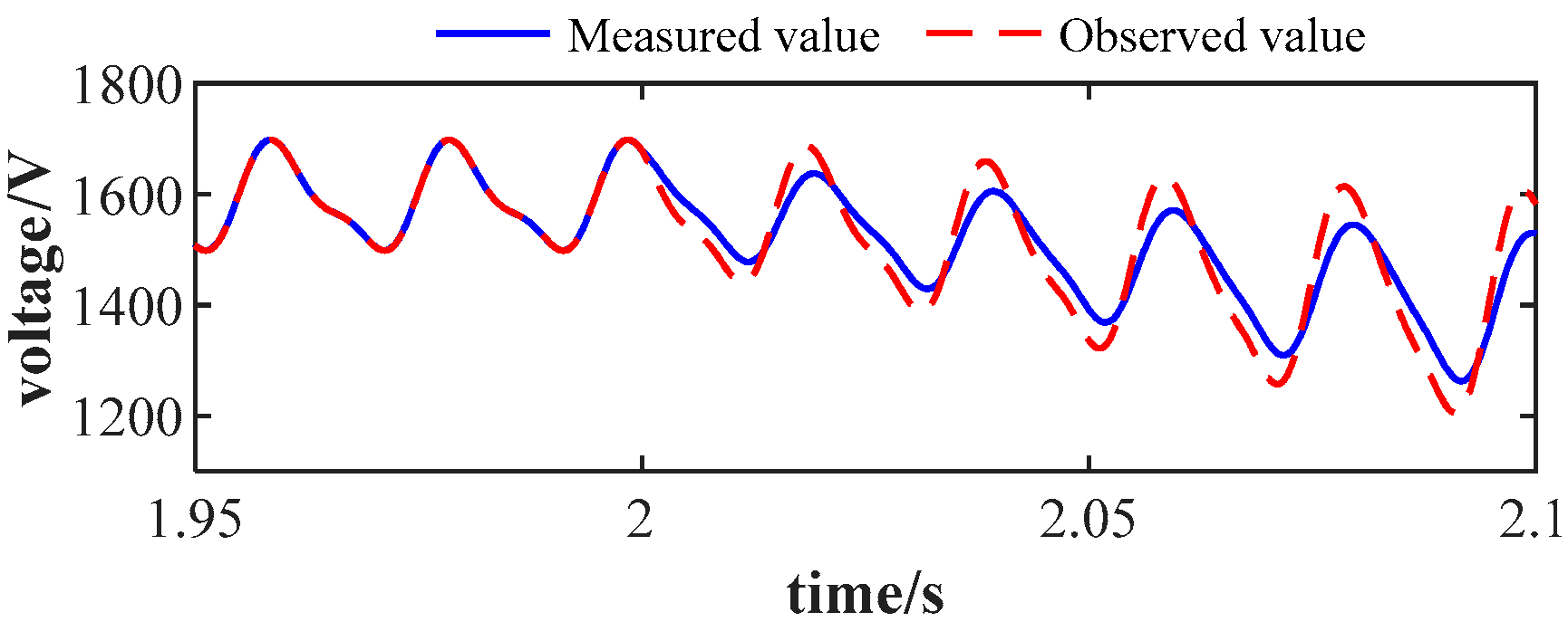
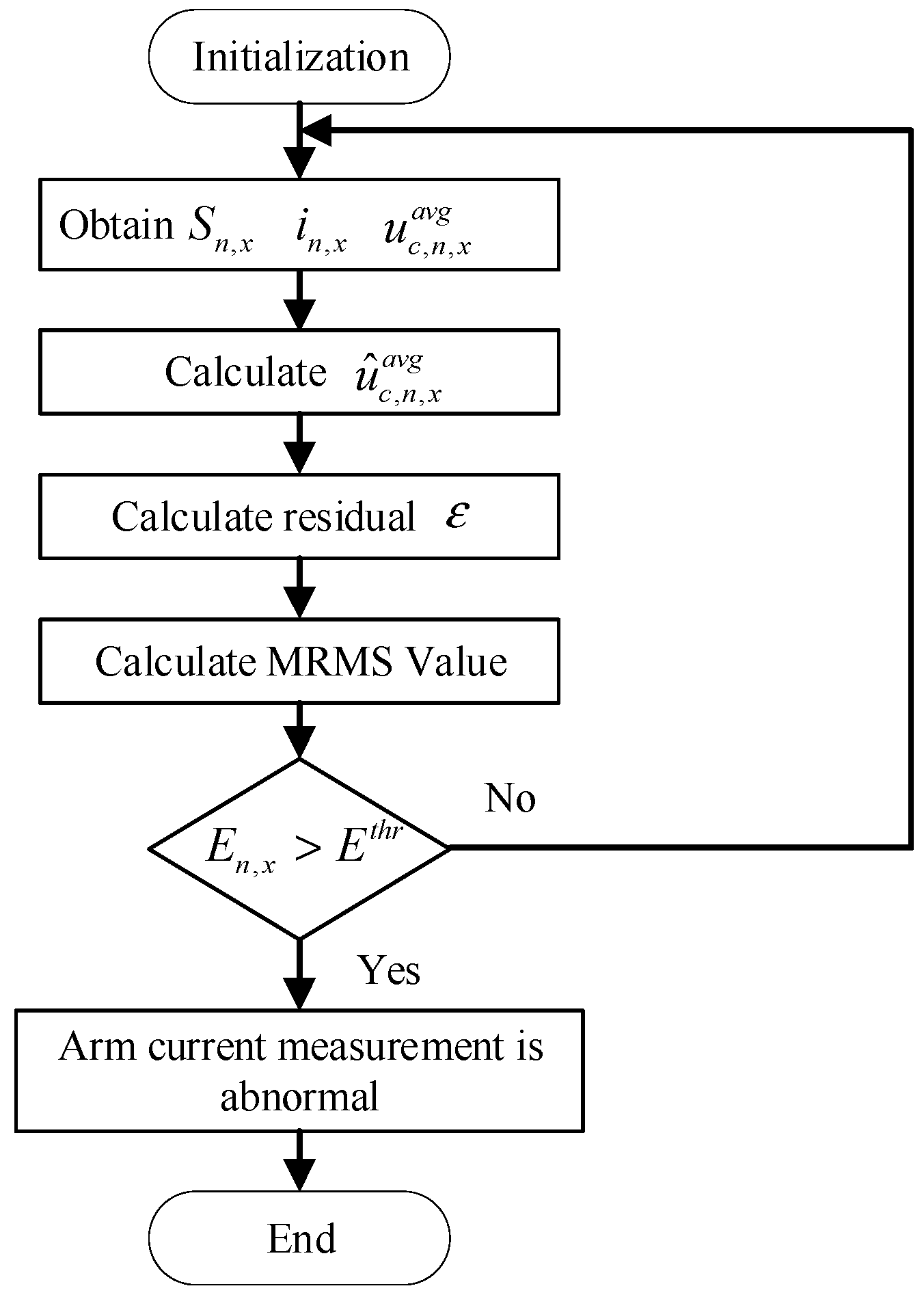
This paper focuses on four typical MMC arm current measurement faults: constant gain faults, amplitude deviation faults, phase shift faults, and stuck faults, along with their detrimental impacts on circulating current control. These faults can induce significant fluctuations in circulating currents, which threaten system stability. To prevent compromised system stability caused by arm current measurement faults, a KF-based fault detection method is proposed. The method selects the SM average capacitor voltage as the observation variable. During normal operation, the observed voltage value converges to the actual value. However, when a fault occurs, the observed voltage value will deviate from the actual voltage. To enhance the fault detection, this paper introduces the Moving Root Mean Square (MRMS) value of the residual. The proposed method allows for the rapid detection of faults in MMC arm current measurement.

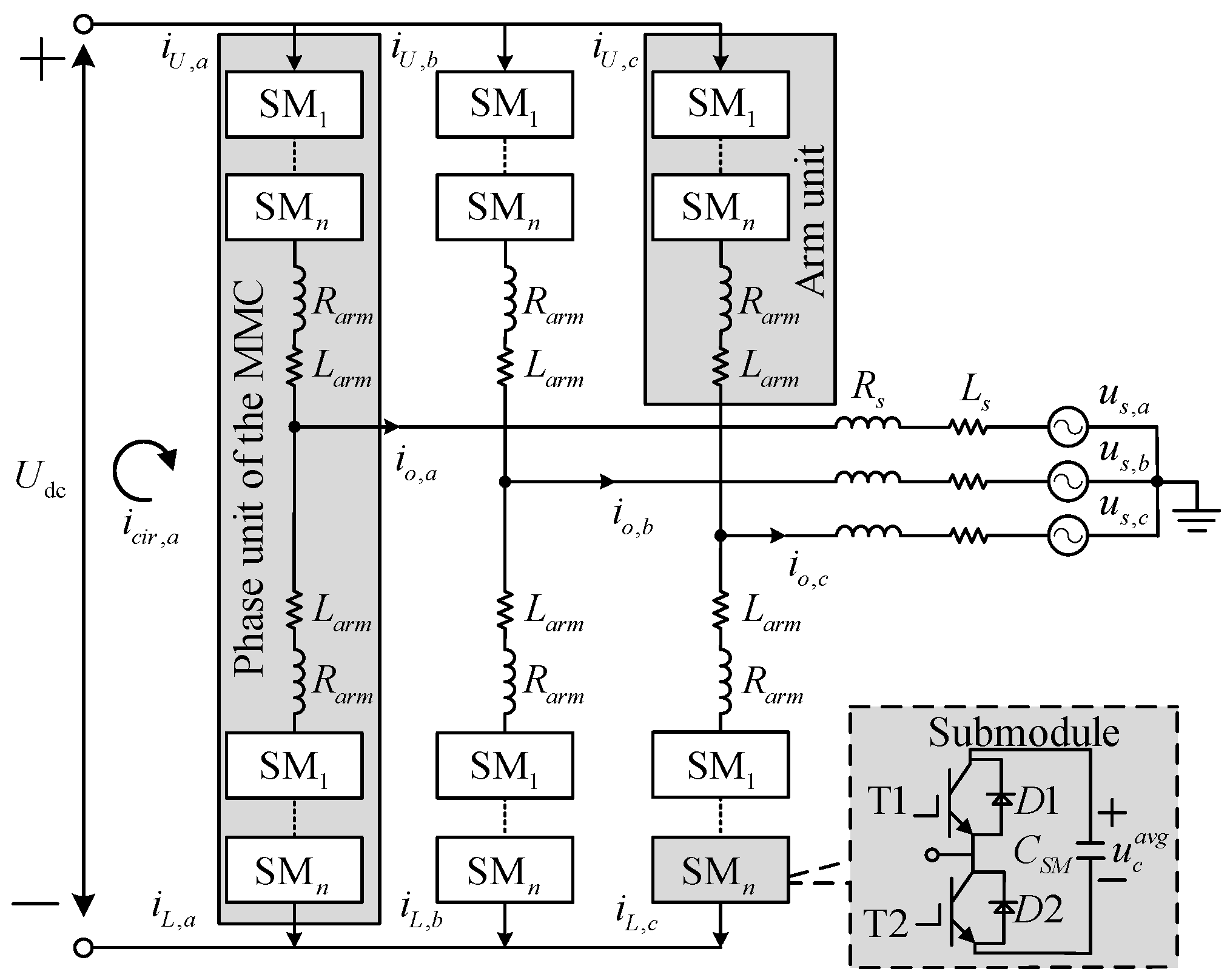
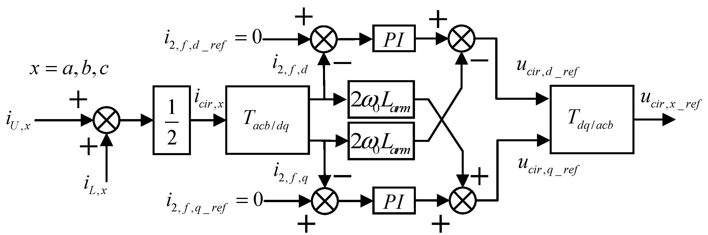
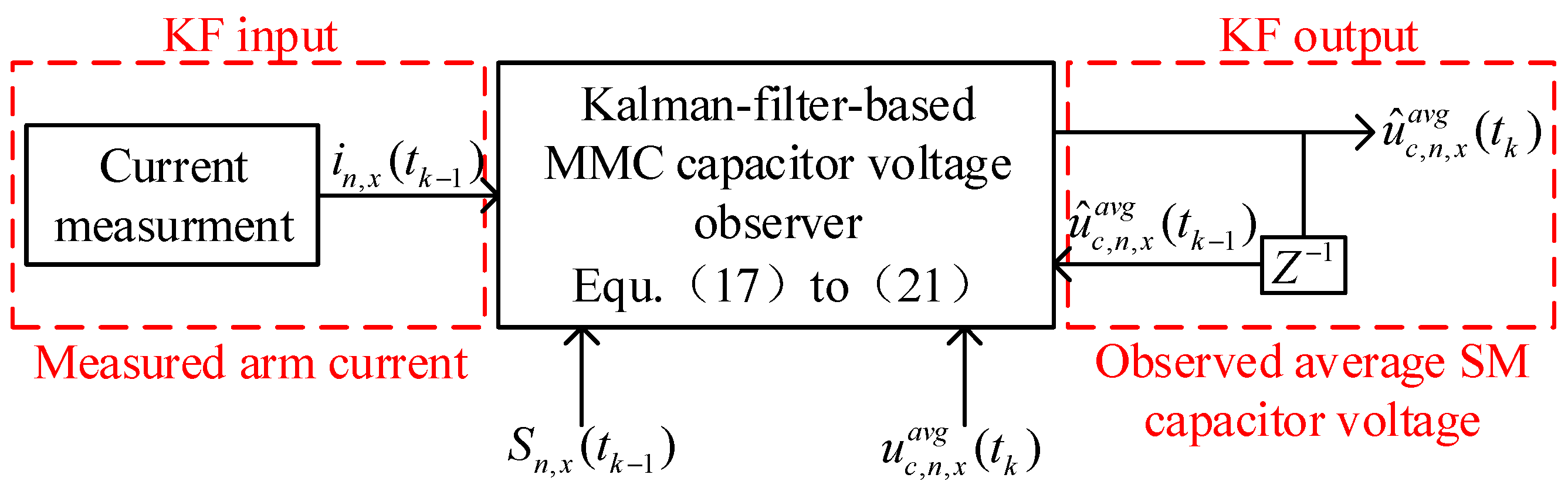
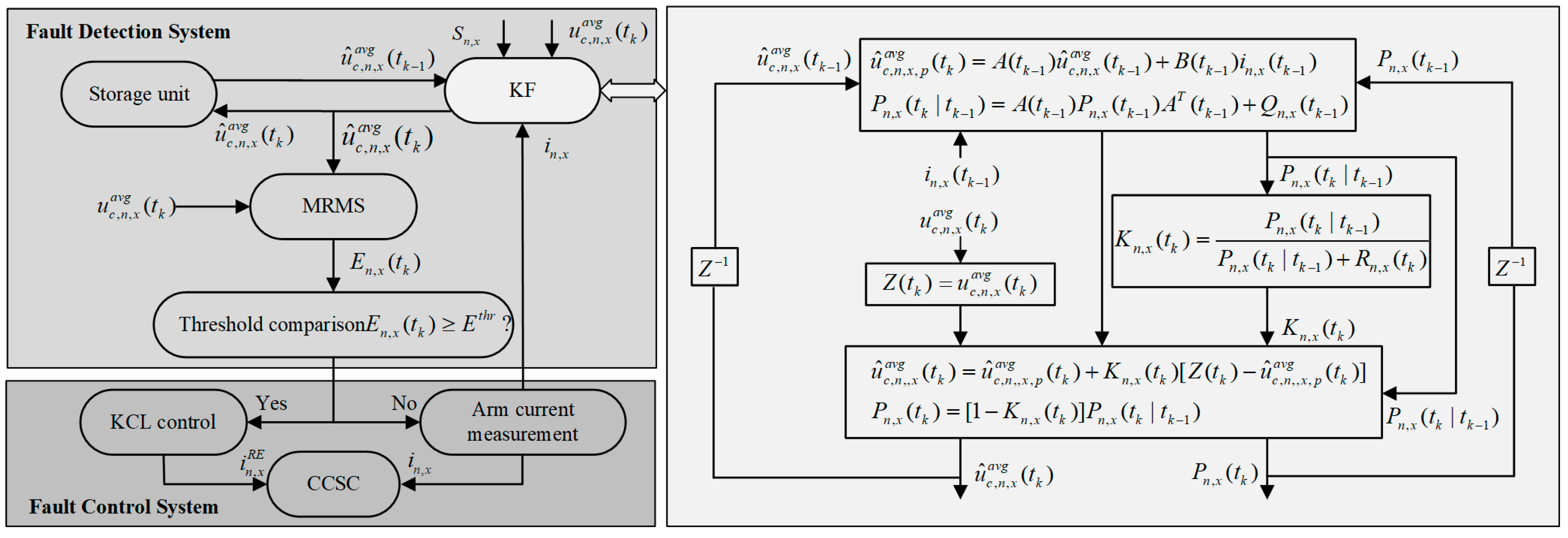
The rest of this paper is organized as follows. Section 2 describes the topology structure of MMCs and the characteristics of circulating current, as well as the dq circulating current suppression controller. Section 3 provides a detailed analysis of four typical arm current measurement faults and their impacts. Section 4 presents the principles of the KF-based fault detection method. Section 5 provides the results of the simulation and experimental validation. Finally, the conclusions are presented in Section 6.

2. MMC Topology and Circulating Current Characteristics

2.1. MMC Operation Principle

The topology of the MMC is shown in Figure 1. The MMC consists of three phases. Each phase consists of two arms: the upper arm and the lower arm. Each arm contains $n$ series-connected SMs, as well as an arm inductor $L_{arm}$ and an arm resistor $R_{arm}$. The half-bridge SM is widely used in existing MMC-HVDC systems, which contain two switching devices and a capacitor.

The relationship between the arm current and SM capacitor voltage is as follows:

$$C_{SM}{\displaystyle \frac{d{u}_{c,n,x,j}}{dt}}=S_{n,x,j}{i}_{n,x}$$

(1)

where $C_{SM}$ is the SM capacitor value, $u_{c,n,x,j}$ and $i_{n,x}$ are the SM capacitor voltage and arm current in phase $x$, $S_{n,x,j}$ is the switch function that controls the charging and discharging of capacitors. Subscripts $n=U,L$ denote the upper and lower arm, respectively, while $j$ indicates the SM index.

The unique structure of MMCs inherently generates circulating currents within each phase, characterized by second-harmonic current components superimposed on the upper and lower arm currents [32].

$$i_{U,x}={\displaystyle \frac{i_{dc}}{3}}+I_1\sin ({\omega }_{0}t+{\phi }_1)+I_{2,f}\cos (2{\omega }_{0}t+{\phi }_2)$$

(2)

$$i_{L,x}={\displaystyle \frac{i_{dc}}{3}}-I_1\sin ({\omega }_{0}t+{\phi }_1)+I_{2,f}\cos (2{\omega }_{0}t+{\phi }_2)$$

(3)

where $i_{dc}$ is the DC current, and $I_1,I_{2,f}$ are the fundamental current amplitude and the second harmonic current amplitude. ${\omega }_0$ is the fundamental angular frequency, and ${\phi }_1,{\phi }_2$ are the initial phase angles of the fundamental current and the second harmonic current, respectively.

Because of the same polarity of the second harmonic current component in the upper and lower arm currents, the common mode current inevitably contains a second harmonic component:

$$i_{cir,x}={\displaystyle \frac{i_{U,x}+i_{L,x}}{2}}={\displaystyle \frac{i_{dc}}{3}}+I_{2,f}\cos (2{\omega }_{0}t+{\phi }_2)$$

(4)

where $i_{cir,x}$ is the circulating current in phase $x$.

2.2. Circulating Current Suppression

The presence of a circulating current not only causes distortion of the arm current but, more critically, it will increase system losses and reduce energy conversion efficiency. In severe cases, it can cause system instability. In order to reduce the harm of the circulating current to the system, it is necessary to adopt the circulating current suppression controller (CCSC) to suppress the circulating current.

The dq frame-based PI controller is a typical CCSC [32], and its structure is shown in Figure 2. From Figure 2, it can be seen that the dq frame-based PI controller requires a circulating current as input to suppress the circulating current, while the acquisition of the current depends on the current measurement device.

3. Impact of Fault on Current Measurement Device

In this section, the four typical arm current measurement faults are discussed, followed by a comprehensive analysis of the fault characteristics and their impacts on the system. The MMC-HVDC simulation model was established in MATLAB/Simulink 2025a to support the analysis. The main parameters of the simulated system are listed in

Table 1. Parameters of Simulation and Experiment Systems.

Parameter	Simulation	Experiment
AC voltage (L-L, RMS)	166 kV	60 V
DC-link voltage	320 kV	120 V
Number of SMs per arm	200	6
Arm inductance	180 mH	6.5 mH
SM capacitance	2.5 mF	1.2 mF
Q for KF	1 × 10−4	1 × 10−4
R for KF	1	1
R Load	/	15 Ω
L Load	/	7.8 mH

, which are based on the Nan’ao multi-terminal project Jinniu station.

The fault of an active DC current measurement device is quite complex. For the convenience of theoretical description and further analysis, the faults occurring in actual operation are classified into constant gain faults, amplitude deviation faults, phase shift faults, and stuck faults. This paper focuses on the above-mentioned four fault types, analyzing their impacts on the MMC three-phase circulating currents and DC current characteristics.

• Constant Gain Fault

The constant gain fault can be characterized as

$$i_{mea}=(1+\alpha )i_{act}$$

(5)

where $i_{mea}$ is the measured value, $i_{act}$ is the actual value, and $\alpha$ is the deviation gain, which can be positive and negative according to the fault characteristics.

Considering the symmetry of MMCs, the upper arm current measurement device in phase $a$ was studied, supposing that $\alpha =\pm 0.1$ and $\alpha =\pm 0.9$ arm current measurement faults occur. The typical dq rotating frame-based CCSC was adopted. Corresponding simulation waveforms are shown in Figure 3 and Figure 4.

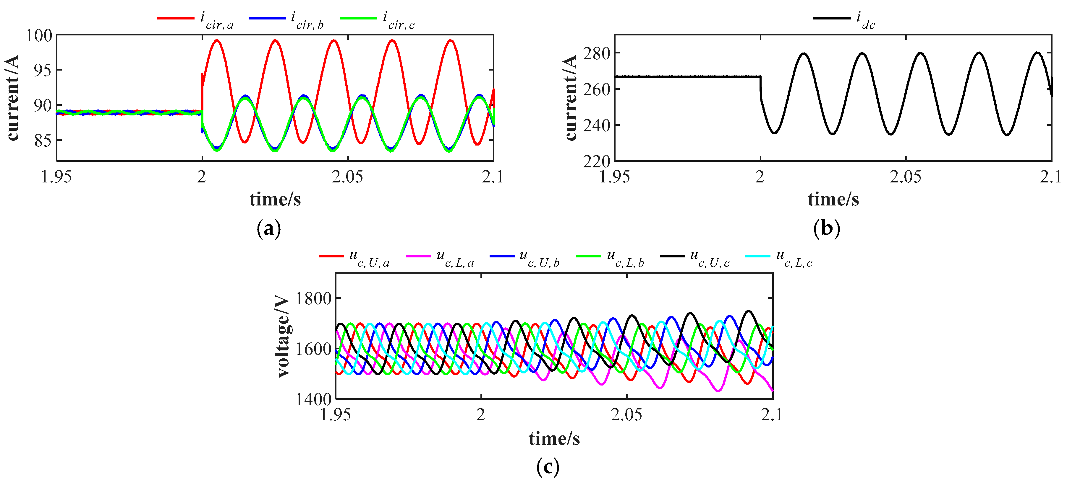
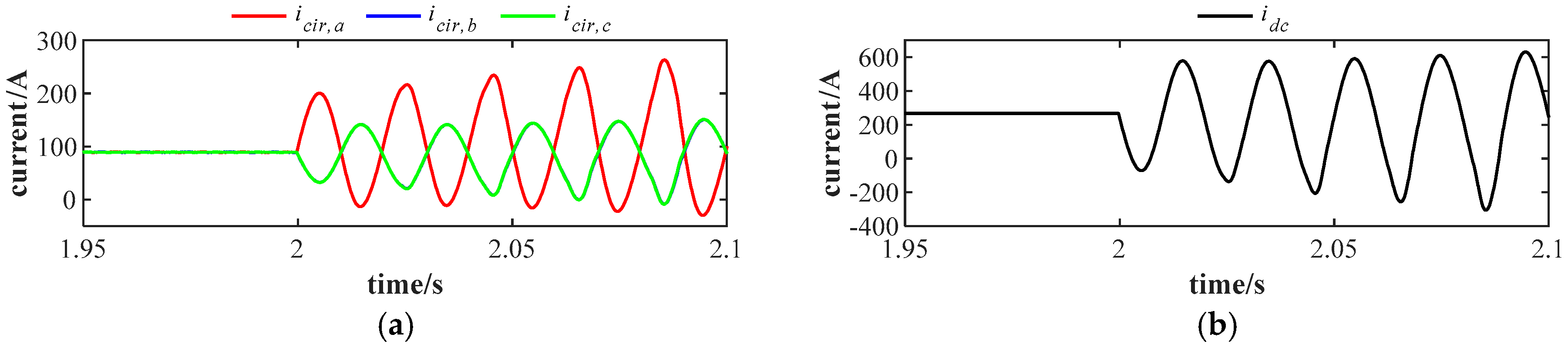
In Figure 3, an $\alpha =-0.1$ arm current measurement fault occurs at 2 s, which means that the arm current value sent to the control system is only 90% of the actual value. Before 2 s, the circulating currents are well mitigated. After that, undesired circulating currents appear. Different from the second-order negative-sequence circulating currents, these currents exhibit zero-sequence characteristics with fundamental frequency. These fundamental frequency oscillating currents also appear on the MMC DC-side, as shown in Figure 3b. 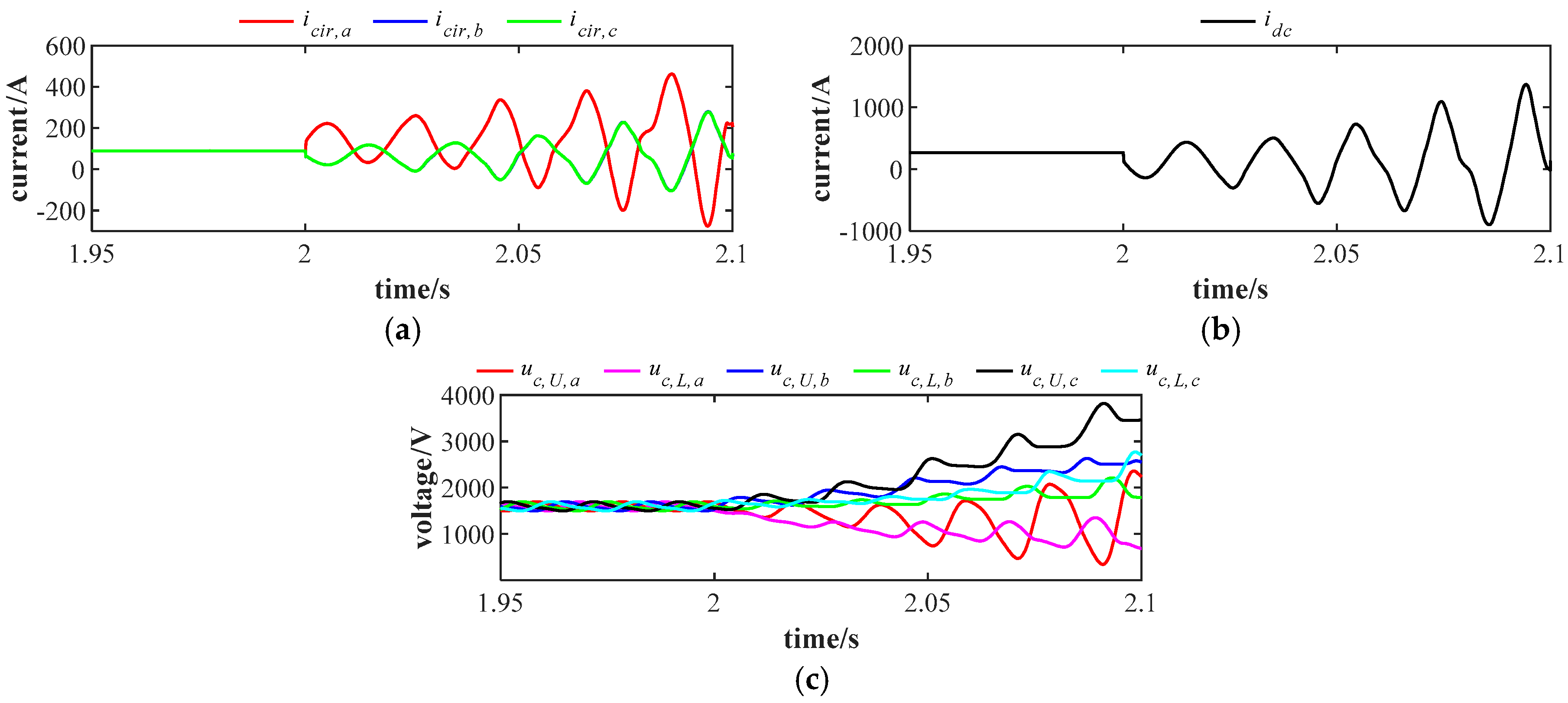The average SM capacitor voltages of six arms are shown in Figure 3c, which are also greatly distorted. Simulation results for the $\alpha =-0.9$ fault case are shown in Figure 4. Severe fault cases induce instability in the MMC. The $\alpha =0.1$ and $\alpha =0.9$ cases simulation results are similar and are not shown here due to page limit.

2.

Amplitude Deviation Faults

The amplitude deviation fault can be characterized as

$$i_{mea}=i_{act}+\beta I_m$$

(6)

where $\beta$ is the amplitude deviation factor, and $I_m$ denotes the arm current amplitude under rated system operating cases. $\beta I_m$ is a constant term; the amplitude deviation fault manifests as a DC component deviation between measured and actual values, with fault severity directly proportional to the absolute value of $\beta$.

When amplitude deviation faults occur, with amplitude deviation faults occur, with $\beta =0.06$ and $\beta =0.33$; the simulation waveforms illustrating the fault impacts are shown in Figure 5 and Figure 6.

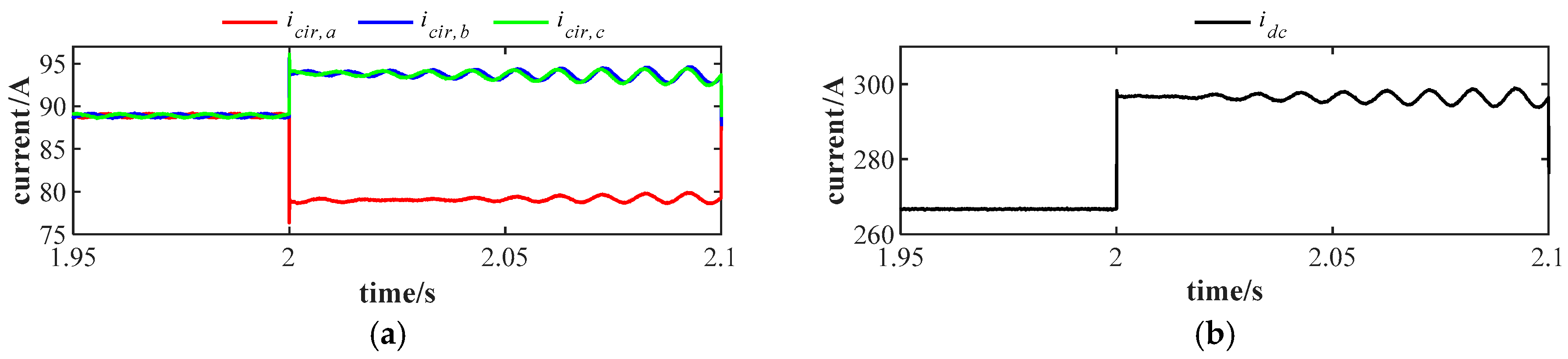
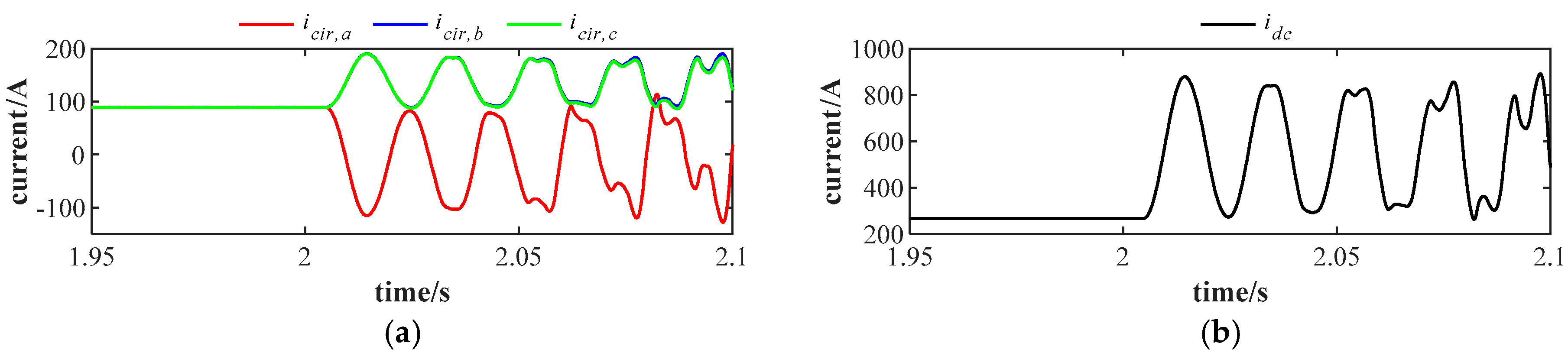
In Figure 5, a $\beta =0.06$ arm current measurement fault occurs at 2 s. At this time, the arm current value sent to the control system is 30 A larger than the actual value. Unlike the constant gain fault, after the occurrence of an amplitude deviation fault, the three-phase circulating currents exhibit significant amplitude steps. Compared to the non-faulty state, the circulating current decreases in phase $a$, while the amplitude of the circulating currents in phases $b$ and $c$ increases. 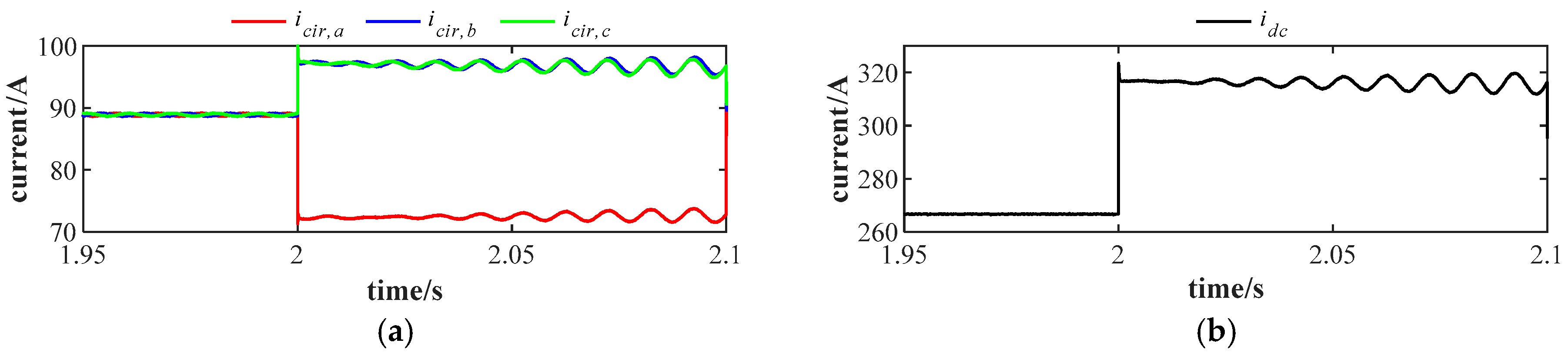The amplitude of the DC current also experiences an amplitude step, as shown in Figure 5b. As the $\beta$ value increases, the three-phase circulating currents and DC current after the fault in Figure 6 exhibit larger amplitude steps compared with those in Figure 5, indicating that the impact of the fault on the MMC system becomes greater.

3.

Phase Shift Faults

The phase shift faults can be characterized as

$$i_{mea}={\displaystyle \frac{i_{dc}}{3}}+I_1\sin ({\omega }_{0}t+{\phi }_1-\gamma \pi )$$

(7)

where $\gamma$ is the phase shift factor, ranging from 0 to 2, which means the phase shift angle spans from 0 to 2π—a full sinusoidal period.

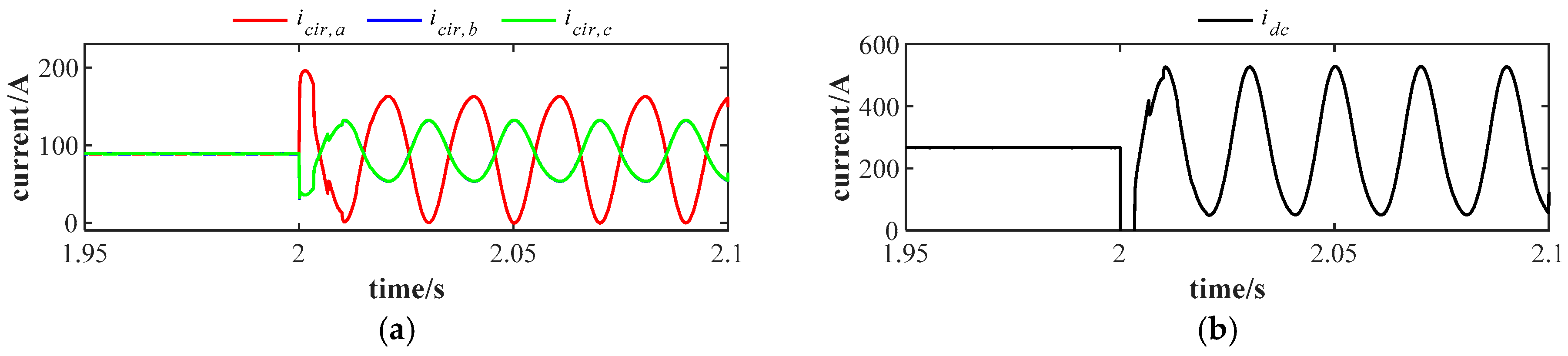
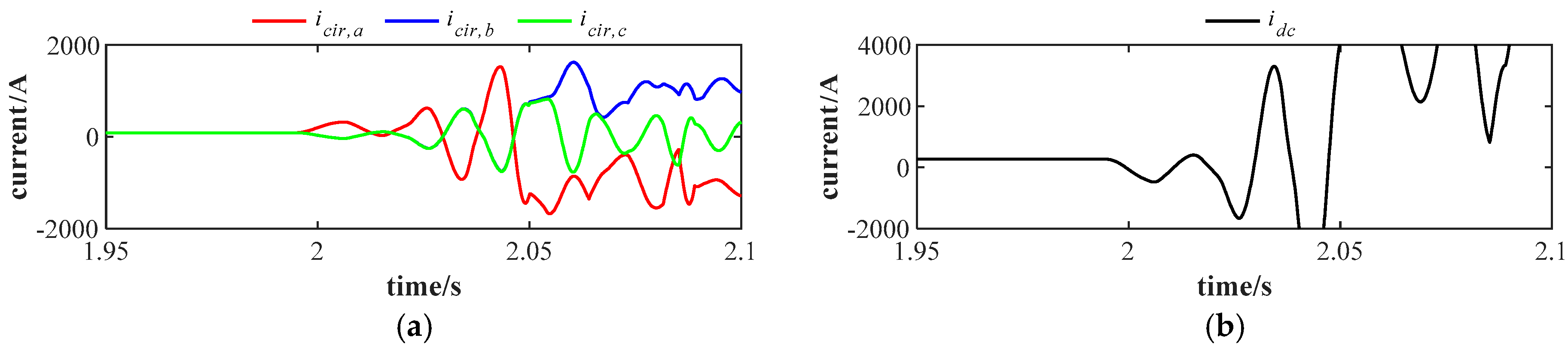
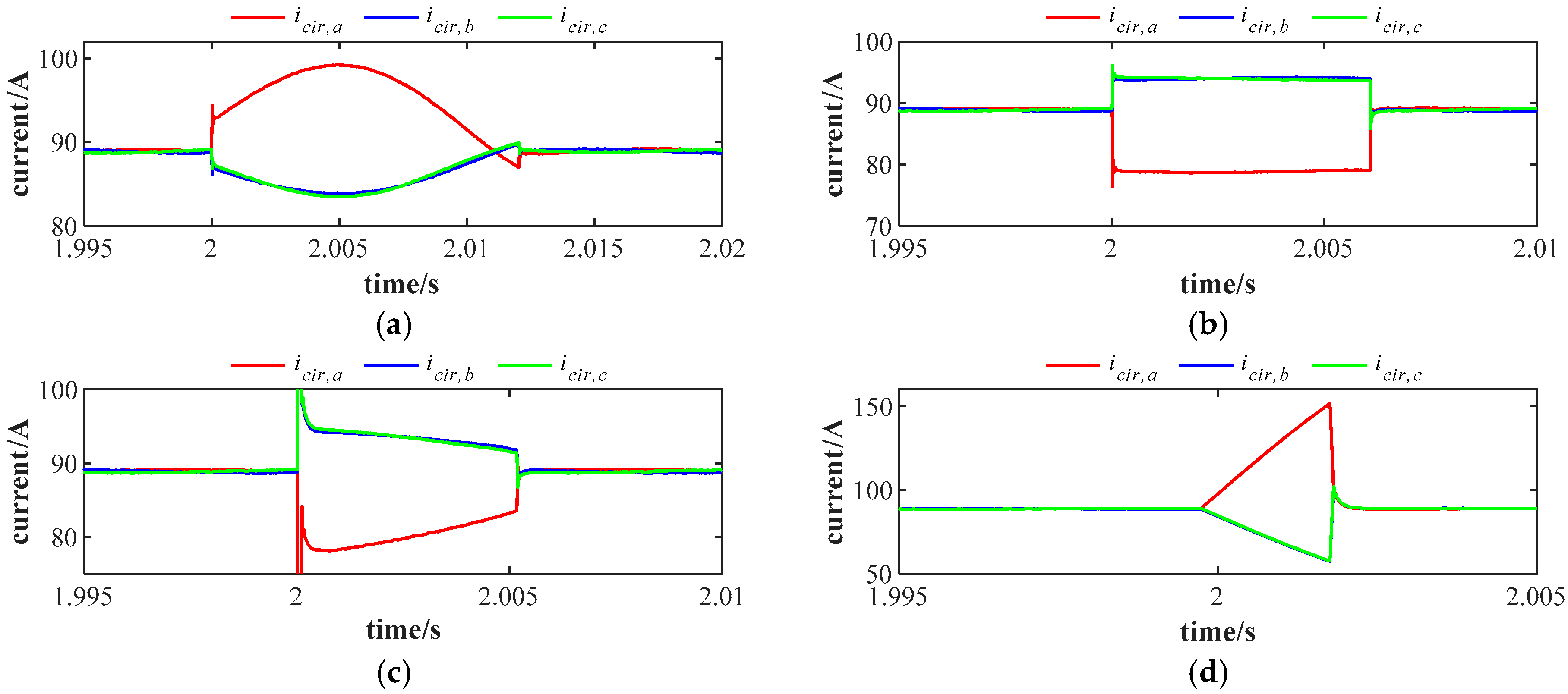
Figure 7 and Figure 8 illustrate the circulating current and DC current waveforms under phase shift faults with $\gamma =1/6$ and $\gamma =1/3$ in the upper arm of phase $a$, respectively. Following the fault occurrence, the three-phase circulating current waveforms exhibit significant fluctuations accompanied by phase shifts. Specifically, the circulating current of phases b and c becomes identical, while that of phase $a$ is phase-shifted by 180 degrees relative to the other two phases. Under a phase shift fault, the DC current will exhibit a fundamental frequency oscillating current. Notably, the amplitude of the fundamental frequency oscillating current increases proportionally with larger phase shift angles.

4.

Stuck Faults

The stuck fault refers to a case where, following the occurrence of a current measurement abnormality, the arm current remains fixed at the value recorded at the fault inception instant.

$$i_{mea}=\lambda I_m$$

(8)

where $\lambda$ is the stuck factor, ranging from −0.26 to 0.66. When $\lambda =0.66$, it indicates a stuck arm current measurement fault when the arm current reaches its maximum value; correspondingly, $\lambda =-0.26$ signifies that the fault occurs at the minimum arm current.

This paper conducts simulation verification on the arm current under stuck fault cases at three characteristic operating points: the maximum value, median value, and minimum value, respectively. The corresponding simulation waveforms are shown in Figure 9, Figure 10 and Figure 11.

Similar to the above-mentioned three fault types, the stuck fault also induces severe fluctuations in both three-phase circulating currents and DC current.

In summary, all four types of faults can trigger pronounced oscillations in three-phase circulating currents. In severe fault cases, the MMC may fail, triggering system protection. To prevent these arm current measurement faults from compromising system stability, it is imperative to develop a rapid fault detection method.

4. Proposed Fault Detection Method

In this section, a general introduction of the KF is given. Subsequently, the relationship equation between the average SM capacitor voltage and arm current is leveraged to derive KF-based fault observation equations. The MRMS technique is then adopted to achieve fault detection.

4.1. Kalman Filter Principle

The KF assumes a linear dynamical system governed by the following equations:

$$X(t_k)=A(t_{k-1})X(t_{k-1})+B(t_{k-1})U(t_{k-1})+w(t_{k-1})$$

(9)

$$Y(t_k)=H(t_k)X(t_k)+v(t_k)$$

(10)

where $X(t_k)$ and $Y(t_k)$ are the system state vector and the measurement vector at time k, $A(t_{k-1})$ denotes the state transition matrix, $B(t_{k-1})$ is the input matrix that maps control inputs $U(t_{k-1})$ to states, $H(t_k)$ is the observation matrix $w(t_{k-1})$, and $v(t_k)$ are the process noise and measurement noise matrix, respectively.

The KF iterates between the prediction phase and the update phase to optimize state estimation. The expressions of the predicted state variable ${\widehat{X}}_p(t_k)$ and the prior error matrix $P(t_k | t_{k-1})$ are written as

$${\widehat{X}}_p(t_k)=A(t_{k-1})\widehat{X}(t_{k-1})+B(t_{k-1})U(t_{k-1})$$

(11)

$$P(t_k | t_{k-1})=A(t_{k-1})P(t_{k-1})A^T(t_{k-1})+Q(t_{k-1})$$

(12)

where $P(t_{k-1})$ and $Q(t_{k-1})$ are the error covariance matrix and the process noise covariance matrix, respectively. During the update phase, the Kalman gain $K(t_k)$ is expressed as

$$K(t_k)={\displaystyle \frac{P(t_k | t_{k-1})H^T(t_k)}{H(t_k)P(t_k | t_{k-1})H^T(t_k)+R(t_k)}}$$

(13)

$R(t_k)$ is the covariance matrix of measurement noise. The Kalman gain is used to update the predicted state variables ${\widehat{X}}_p(t_k)$ and error covariance matrix $P(t_{k-1})$. The update equation is expressed as

$$\widehat{X}(t_k)={\widehat{X}}_p(t_k)+K(t_k)[Z(t_k)-H(t_k){\widehat{X}}_p(t_k)]$$

(14)

$$P(t_k)=[I-K(t_k)H(t_k)]P(t_k | t_{k-1})$$

(15)

where $Z(t_k)$ is the actual measured values of output variables. $\widehat{X}(t_k)$ is the update state variables, and I is the identity matrix. After the update, the algorithm advances to the subsequent time step k + 1 and recursively iterates the prediction–correction cycle.

4.2. KF-Based Fault Detection Method

In MMCs, the arm current charges and discharges the SM capacitor voltages according to the current direction. This relation can be described as follows

$$C_{SM}{\displaystyle \frac{d{u}_{c,n,x}^{avg}}{dt}}=S_{n,x}{i}_{n,x}$$

(16)

where $u_{c,n,x}^{avg}$ is the average SM capacitor voltage in one arm, $i_{n,x}$ is the arm current, $S_{n,x}$ is the corresponding switching function, and $C_{SM}$ is the SM capacitance. Subscripts $n=U,L$ and $x=a,b,c$ denote the upper and lower arm, in three phases, respectively.

Use the forward Euler approximation to (16), and choose the average SM capacitor voltage in one arm as the predicted state variable and output variable, and the arm current as the input variable. Then, the prediction equation can be written as

$${\widehat{u}}_{c,n,x,p}^{avg}(t_k)={\widehat{u}}_{c,n,x}^{avg}(t_{k-1})+{\displaystyle \frac{T_s}{C_{sm}}}{S}_{n,x}(t_{k-1})i_{n,x}(t_{k-1})$$

(17)

And corresponding update equations based on KF theory are given as follows

$$P_{n,x}(t_k | t_{k-1})=P_{n,x}(t_{k-1})+Q_{n,x}(t_{k-1})$$

(18)

$$K_{n,x}(t_k)={\displaystyle \frac{P_{n,x}(t_k | t_{k-1})}{P_{n,x}(t_k | t_{k-1})+R_{n,x}(t_k)}}$$

(19)

$${\widehat{u}}_{c,n,x}^{avg}(t_k)={\widehat{u}}_{c,n,x,p}^{avg}(t_k)+K_{n,x}(t_k)[u_{c,n,x}^{avg}(t_k)-{\widehat{u}}_{c,n,x,p}^{avg}(t_k)]$$

(20)

$$P_{n,x}(t_k)=[1-K_{n,x}(t_k)]P_{n,x}(t_k | t_{k-1})$$

(21)

where ${\widehat{u}}_{c,n,x,p}^{avg}(t_k)$ is the predicted capacitor voltage, ${\widehat{u}}_{c,n,x}^{avg}(t_k)$ is the updated capacitor voltage, and $u_{c,n,x}^{avg}(t_k)$ is the actual measured capacitor voltage.

Based on (17) to (21), six average MMC SM capacitor voltages can be observed simultaneously in real time.

In summary, in the proposed observation process, the MMC arm current serves as the input to the KF, and the SM capacitor voltage serves as the output of the KF, as illustrated in Figure 12.

4.3. Voltage Observation

The effectiveness of the KF in observing the average SM capacitor voltage is initially confirmed. Figure 13 illustrates the time-domain simulation waveforms of both the actual and predicted capacitor voltages. In Figure 13a, when a step change in reactive power is applied at 2 s, the predicted voltage closely aligns with the actual voltage, demonstrating the accuracy of the KF. Figure 13b depicts a phase-to-ground fault simulation, further validating the KF’s reliability. In normal operation, the KF observation residuals ${\epsilon }_{n,x}$ are small.

$${\epsilon }_{n,x}(t_k)=u_{c,n,x}^{avg}(t_k)-{\widehat{u}}_{c,n,x}^{avg}(t_k)$$

(22)

4.4. MRMS Value of the Residual

When a fault occurs in the arm current measurement, the input of the KF will be jeopardized, resulting in a significant increase in the observation residual. Figure 14 shows the observation of the average SM capacitor voltage in fault cases. A $\alpha =-0.5$ constant gain fault occurs at 2 s, causing the observed value to deviate from the measured value.

However, the observation residual can be either positive or negative and usually displays a periodic pattern, complicating the establishment of an appropriate fault detection threshold.

In this paper, the MRMS value of the residual $E_{n,x}$ is defined, which can be calculated by

$$E_{n,x}(t)=\sqrt{{\displaystyle \frac{1}{\Delta t}}{\displaystyle {\int }_{t-\Delta t}^t{\epsilon }_{n,x}^{2}dt}}$$

(23)

where $\Delta t$ is the integration interval. Based on (23), the MRMS value between $[t-\Delta t,t]$ is obtained and refreshed in real time. The integral operation has a good suppression effect on the system noise and can avoid false detection. Then, compare $E_{n,x}$ with the detection threshold $E^{thr}$. Once it exceeds the $E^{thr}$, the arm current measurement fault in phase $x$ arm $n$ is detected. The entire fault detection process is shown in Figure 15.

4.5. Overall Design

The block diagram of the proposed method is depicted in Figure 16. Relevant circuit and control variables are sent to six voltage KF observers. Subsequently, the MRMS values are calculated. By comparing these MRMS values with a predefined threshold, the occurrence of an arm current measurement fault can be determined.

After the fault detection, Kirchhoff’s Current Law (KCL) is employed to correct the measurement error. For example, if the upper arm current of phase $a$, $i_{U,a}$ is faulty, it can be immediately replaced by the other accurate measurement results

$$i_{U,a}^{RE}=i_{dc}-i_{U,b}-i_{U,c}$$

(24)

5. Simulation and Experimental Verification

In this section, the proposed fault detection method is verified through both simulation and experimental results.

5.1. MRMS and Fault Detection

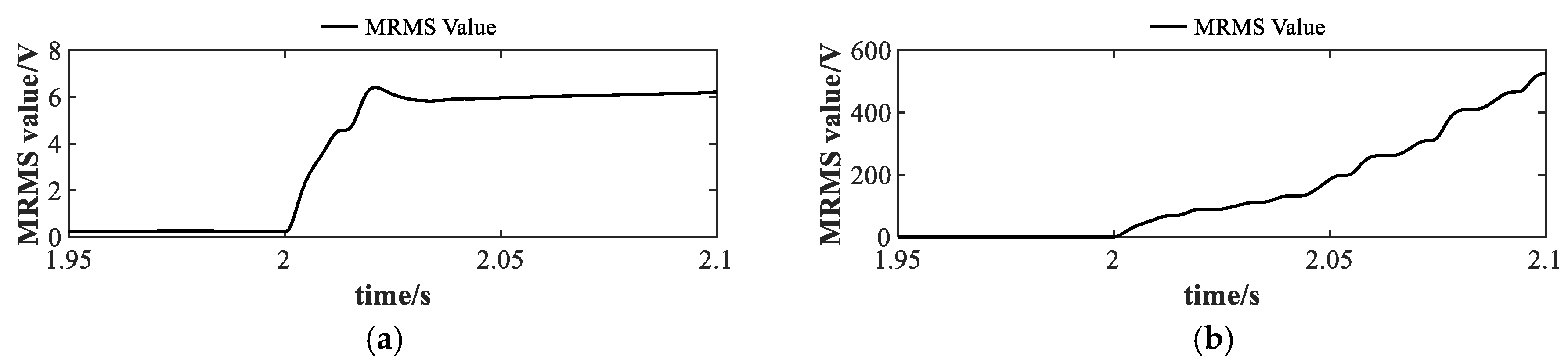
Figure 17 shows the MRMS value of the SM capacitor voltage observation residual. In this paper, the integration interval is set to 20 ms. Before 2 s, the MRMS value is almost zero. When an arm current measurement fault occurs, it quickly reaches a high level, making it a good fault indicator.

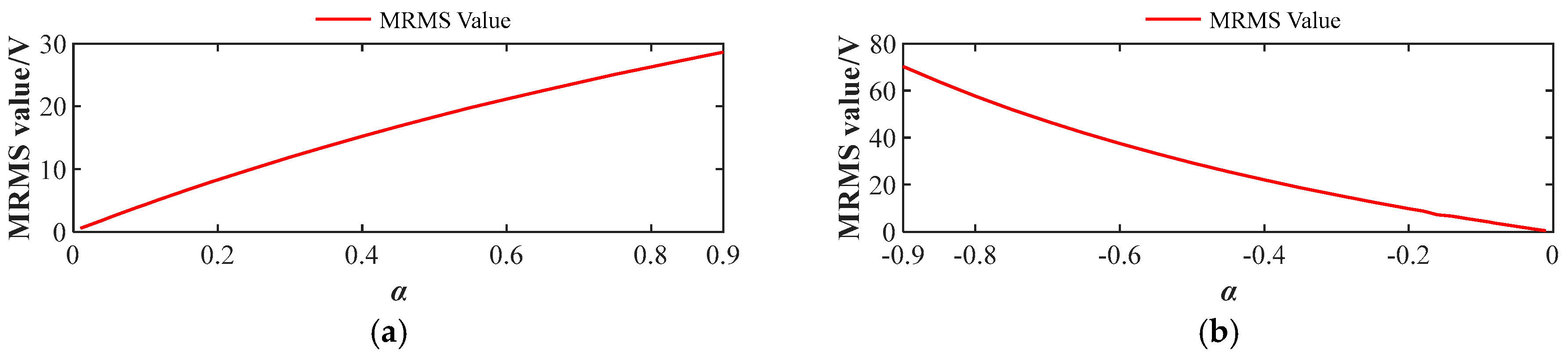
To further illustrate the relationship between MRMS values of the residual and the degree of fault, Figure 18 displays MRMS values under a constant gain fault case with different $\alpha$. As the severity of the fault increases, the MRMS residual increases correspondingly. Moreover, negative deviation faults have a larger impact on the MMC and are more likely to cause instability. Based on Figure 18, a proper detection threshold $E^{\mathrm{thr}}$ can be selected according to the desired arm current measurement fault detection sensitivity.

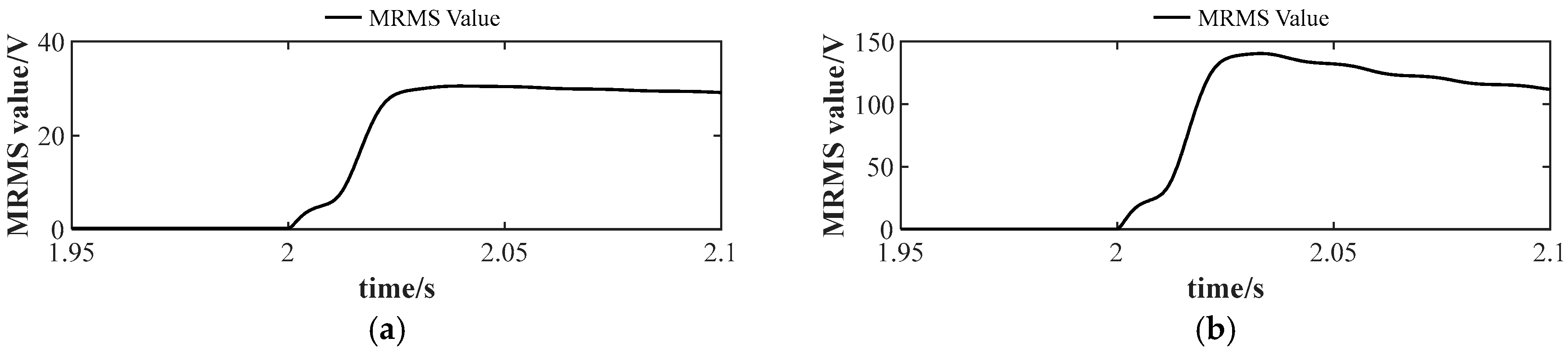
Figure 19 shows the MRMS value of the SM capacitor voltage observation residual under the amplitude deviation fault. Similar to the case of constant gain fault, when the system is under normal case 2 s before, the MRMS value nears 0. When an arm current measurement fault occurs at 2 s, the MRMS value rapidly increases, which can effectively detect the occurrence of the fault.

Figure 20 displays the MRMS value under the amplitude deviation fault case with different $\beta$. As the severity of the fault increases, the MRMS values also increase accordingly. Fault severity is positively correlated with the MRMS value; the higher the severity of the fault, the easier it is to detect it.

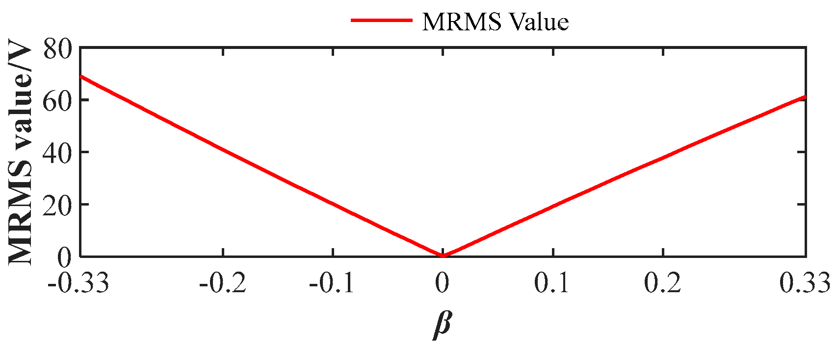
Upon the occurrence of a phase shift fault, the MRMS value rapidly increases from near 0 to a stabilized plateau level. As shown in Figure 21a,b, the plateau value of the MRMS exhibits a positive correlation with the phase shift angle magnitude. This relationship is further validated in Figure 22, where the plateau value linearly increases with phase shift factor up to $7/9$, accompanied by escalating fault severity. The MRMS value reaches its global maximum at $\gamma =7/9$. Beyond $\gamma =7/9$, the MRMS plateau value decreases progressively with increasing phase shift factor. At $\gamma =2$, the arm current completes a full-cycle displacement, resulting in phase realignment with the normal operating case. Consequently, the MRMS value converges to its baseline level observed at $\gamma =2$.

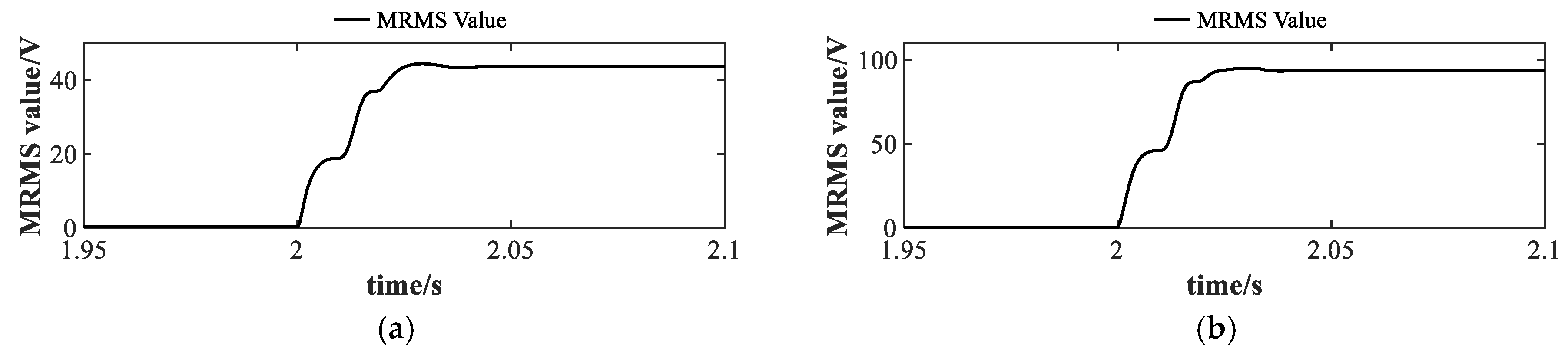
Figure 23 presents the MRMS values under different stuck fault cases. Consistent with the above-mentioned fault scenarios, the MRMS exhibits a significant surge immediately following the fault inception, enabling effective detection of the fault occurrence.

Through Figure 24, the relationship between the MRMS value and $\lambda$ under the stuck fault case can be visually understood.

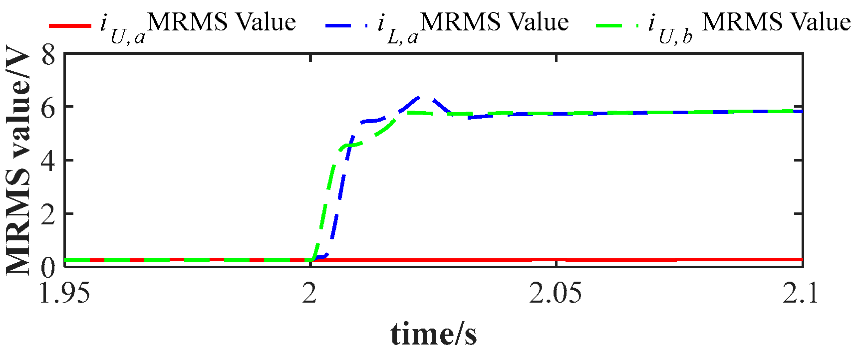
Figure 25, Figure 26 and Figure 27 are provided to explore the impact of one arm current measurement fault on the KF observation in other arms. Figure 25 illustrates the MRMS waveform when the normal current measurement in the upper arm of phase $a$ and the lower arm of phase $a$ experiences a constant gain fault with $\alpha =-0.1$. Following the fault occurrence at 2 s, the MRMS value of the lower arm of phase $a$ rises rapidly, whereas the MRMS value of the upper arm of phase $a$ remains unchanged and near 0, indicating no interference from faults in the adjacent arm within the same phase.

Figure 26 and Figure 27 present the MRMS waveforms under two experimental cases: (1) normal current measurement in the upper arm of phase $a$ with a $\alpha =-0.1$ constant gain fault in the upper arm of phase $b$; and (2) normal current measurement in the upper arm of phase $a$ with simultaneous $\alpha =-0.1$ constant gain faults in both the lower arm of phase $a$ and the upper arm of phase $b$ at 2 s. Both conclusions from Figure 26 and Figure 27 confirm that neither adjacent arm measurement faults in the same phase nor arm measurement faults in different phases affect the KF observation. These results validate the independence of the proposed method.

Based on the MRMS values observed across all the above-mentioned fault scenarios, the detection threshold must be selected to ensure the identification of all fault cases. Based on the analysis, a 4.5 V threshold is set. The fault occurrence is conclusively diagnosed when the MRMS value exceeds this threshold.

5.2. Fault Control

Figure 28 demonstrates the circulating current waveforms under four fault scenarios before and after implementing the KCL-based control strategy. Prior to the fault occurrence, the three-phase circulating currents exhibit only a DC component. Following the fault initiation, harmonics emerge in the circulating currents, inducing waveform distortion and triggering MRMS values to increase. Upon exceeding the 4.5 V threshold, the KCL-based control is activated, which rapidly suppresses the harmonic components and restores the circulating currents to their normal state. These simulation results validate the effectiveness of both the fault detection methodology and the KCL control strategy.

5.3. Discussion

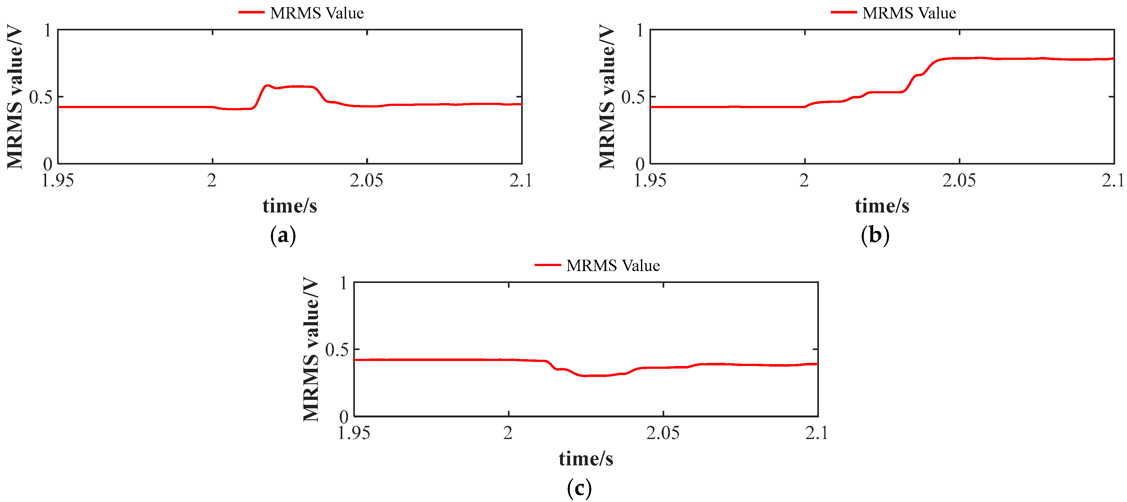
To further verify the robustness of the proposed method, Figure 29 presents the MRMS values under active power changing, reactive power changing, and phase-to-ground fault cases. Figure 29a shows the MRMS waveform under the power changing case, where at 2 s, the system’s reactive current changes from 0 A to 200 A. Figure 29b shows the MRMS waveform under the active power changing case, where at 2 s, the DC load steps. Figure 29c shows the MRMS waveform under the phase-to-ground fault case, where at 2 s, a single phase-to-ground fault occurs on phase $a$. In all cases, when a fault occurs, the MRMS value only experiences small fluctuations and does not affect the detection result.

In addition, the impact of measurement noise is also analyzed. According to the national standards for DC current measurement devices in China [33], these devices have multiple standard accuracy levels. In this study, a typical DC current measurement device with an accuracy level of 0.1 (highest) is considered. Therefore, a 0.1% measurement noise during the measurement process is introduced. Figure 30 shows the MRMS waveforms under both conditions: without measurement noise and with measurement noise. When no measurement noise is added, the MRMS without faults is approximately 0.4 V. After adding measurement noise, the MRMS value remains close to that of the case without measurement noise, which confirms the robustness against noise.

5.4. Experimental Results

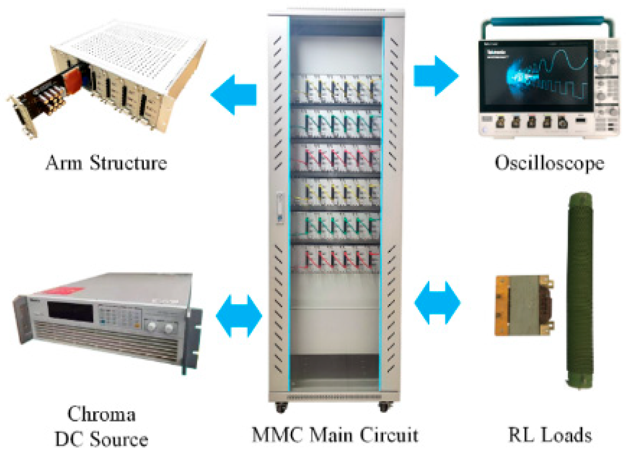
Figure 31 illustrates the designed experimental platform. The MMC is powered by a voltage source and drives RL loads. The typical dq frame-based circulating current control method is employed.

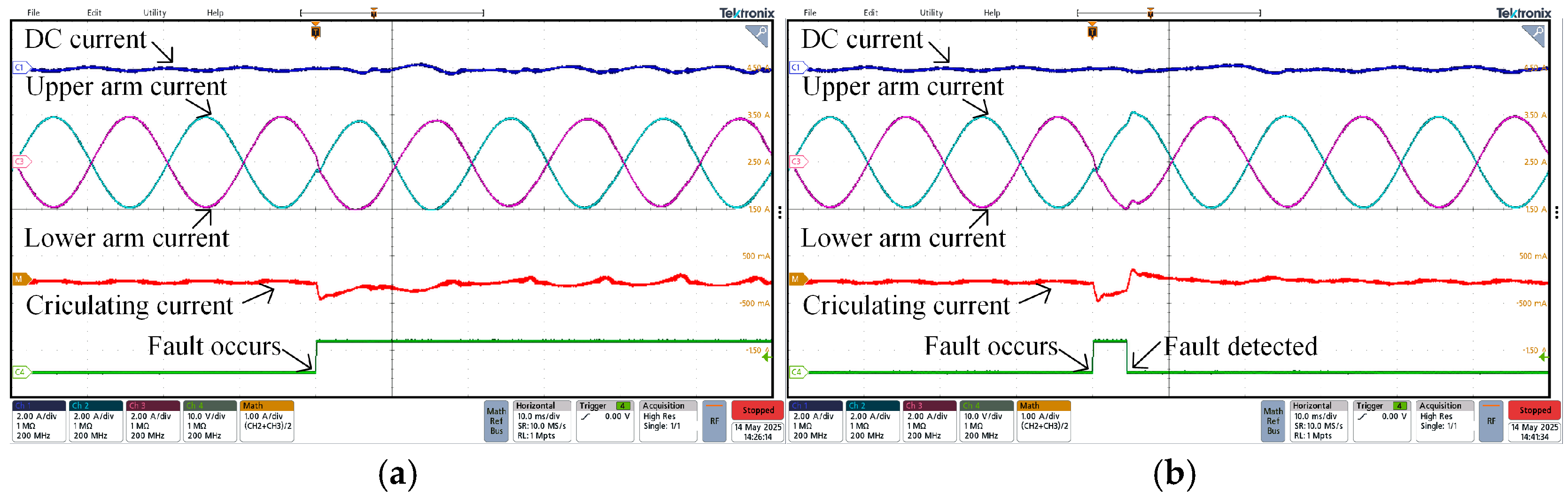
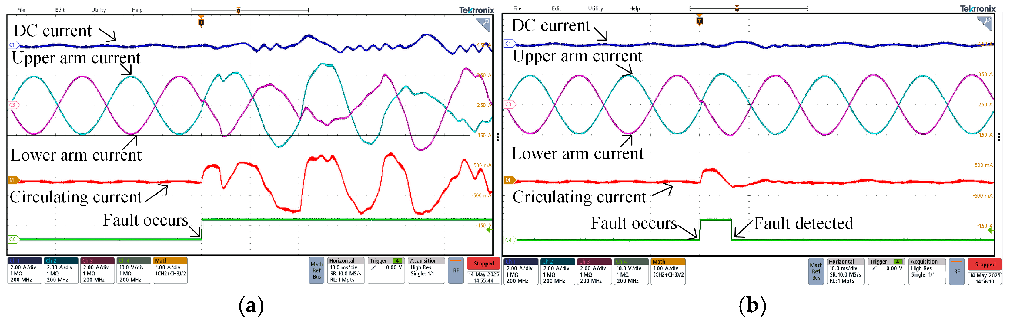
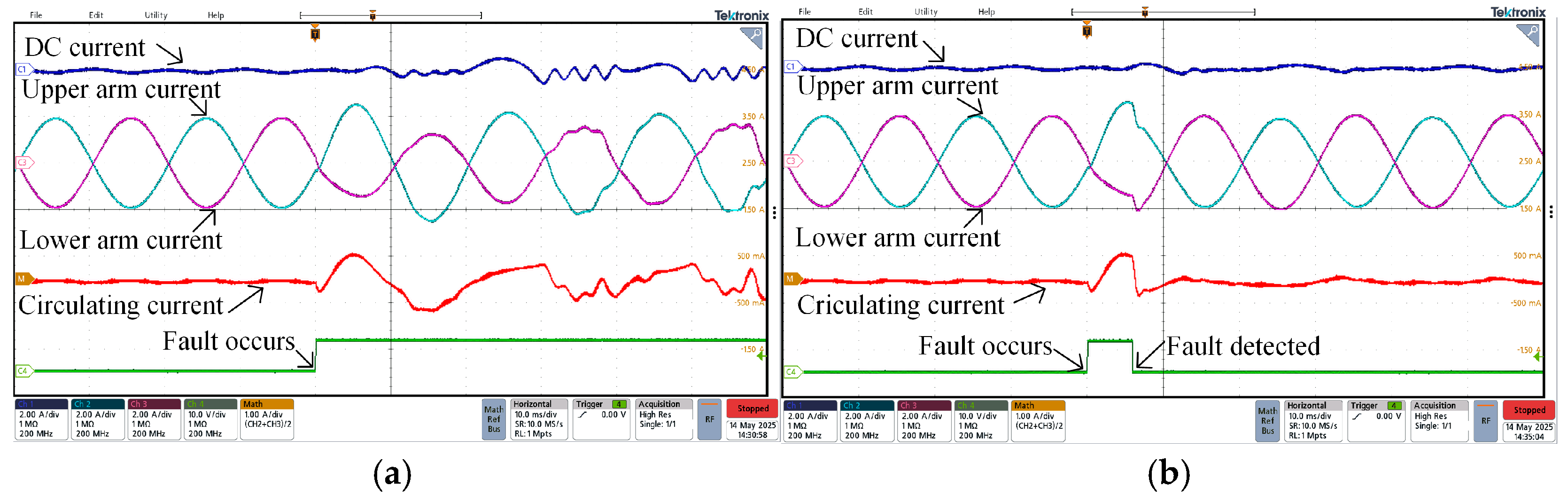
Figure 32, Figure 33, Figure 34 and Figure 35 illustrate the fault impacts of four arm current measurement faults on the DC current, upper and lower arm currents of the $a$ phase, and circulating currents, as well as the experimental waveforms of fault detection and KCL control. Figure 32a,b show the fault impact, fault detection, and control experimental waveforms at $\alpha =0.5$, respectively. Experiments demonstrate that the proposed method can detect measurement faults within 10 ms. When the MRMS reaches the threshold, KCL control is activated, and the circulating current recovers to normal. Figure 33a,b present the fault impact and fault detection experimental waveforms under an amplitude deviation fault of $\beta =0.5$. After the fault occurs, the DC current and circulating current fluctuate. After engaging fault detection and control, the fault is mitigated, and the system restores stable operation within approximately 5 ms.

In Figure 34 and Figure 35, when arm measurement occurs in phase shift faults and stuck faults, although both faults have more severe impacts on the DC current and circulating current, the proposed strategy can still stabilize the MMC system within approximately 7 ms after introducing fault control.

These experimental results validate the effectiveness of the proposed KF-based fault detection method and KCL control method.

5.5. Discussion of Limitations

For the simulation system:

First, the simulation platform operates with discrete time steps, which limits its ability to fully replicate the continuous dynamics of real MMC systems. Second, in the simulation, the Half-Bridge MMC module provided by Simulink is used, which is an equivalent model that ignores the switching characteristics.

For the experimental system:

First, the experimental platform is a low-voltage, low-power downscaled prototype, whereas practical MMC-HVDC systems typically operate at several hundred kilovolts. As such, the experimental results primarily provide qualitative validation. Moreover, in the laboratory setup, all necessary signals are directly routed to the DSP for processing, without accounting for the multi-level controller communication in actual systems.

6. Conclusions

This paper investigates the impact of four critical arm current measurement faults on MMC operation. These faults induce undesirable harmonic currents into the circulating current, threatening system reliability. To address this issue, a fault detection method based on the KF is proposed. This method uses the arm measurement current as the input of the KF. By constructing an arm dynamics model and implementing KF equations, the average capacitor voltage of the SM can be observed in real time. The MRMS value is employed to simplify the fault detection process: when the MRMS value of observation residuals exceeds a predefined threshold, within 20 ms, the arm current measurement fault is identified. After fault detection, a KCL control strategy is utilized to mitigate fault impacts. This method can quickly and independently detect whether there are any abnormalities in the current measurements of the six arms of the MMC. Both simulations and experiments validate the effectiveness of the proposed method.