Abstract
Gas turbine (GT) modeling and optimization have been widely studied at the design level but still lacks focus on real-world operational cases. The concept of a digital twin (DT) allows for the interaction between operation data and the system dynamic performance. Among many DT studies, only a few focus on GT for thermal power plants. This study proposes a digital twin prototype framework including the following modules: process modeling, parameter estimation, and performance optimization. Provided with real-world power plant operational data, key performance parameters such as turbine inlet temperature (TIT) and specific fuel consumption (SFC) were initially unavailable, therefore necessitating further calculation using thermodynamic analysis. These parameters are then used as a target label for developing artificial neural networks (ANNs). Three ANN models with different structures are developed to predict TIT, SFC, and turbine power output (GTPO), achieving high R2 scores of 94.03%, 82.27%, and 97.59%, respectively. Physics-informed neural networks (PINNs) are then employed to estimate the values of the air–fuel ratio and combustion efficiency for each time index. The PINN-based estimation resulted in estimated values that align with the literature. Subsequently, an unconventional method of detecting alarms by using conformal prediction were also proposed, resulting in a significantly reduced number of alarms. The developed ANNs are then combined with particle swarm optimization (PSO) to carry out performance optimization in real time. GTPO and SFC are selected as the primary metrics for the optimization, with controllable parameters such as AFR and a fine-tuned inlet guide vane position. The results demonstrated that GTPO could be optimized with the application of conformal prediction when the true GTPO is detected to be higher than the upper range of GTPO obtained from the ANN model with a conformal prediction of a 95% confidence level. Multiple PSO variants were also compared and benchmarked to ensure an enhanced performance. The proposed PSO in this study has a lower mean loss compared to GEP. Furthermore, PSO has a lower computational cost compared to RS for hyperparameter tuning, as shown in this study. Ultimately, the proposed methods aim to enhance GT operations via a data-driven digital twin concept combination of deep learning and optimization algorithms.
1. Introduction
As a critical technology providing a clean, highly efficient, and cost-effective power generation for thermal power plants, the gas turbine (GT) remains prone towards performance deterioration over a prolonged period of operations [1]. This deterioration not only affects the power output, but also increases emissions and operational risks. It is commonly classified into two types, namely gas path faults (e.g., blade or vane fouling, corrosion, and erosion) and mechanical faults (e.g., rotor dynamic imbalance, eccentricity, bearing failures, and rotor cracks) [2,3,4,5]. Such faults typically lead to abnormal deviations in the sensor readings [6], negatively impacting efficiency. To maintain optimal GT performance, it is essential to operate the system under conditions that minimize fuel consumption and maintenance costs while maximizing power output.
Engine health monitoring (EHM) has been providing benefits to operators by reducing costs and downtime, extending use life, improving safety, and reducing fuel consumption [7]. However, traditional EHM systems are typically reactive, relying on threshold-based alarms and periodic maintenance, which often fail to capture early-stage faults or adapt to dynamic operational regimes. The rising operations and maintenance (O&M) costs (e.g., USD 36 billion in 2024 and growing at annual growth rate of 3.8% [8]) highlight the urgent need for proactive and adaptive solutions. This raises a critical question: What factors are driving this increase? A possible explanation lies in the limitation of existing EHM systems, which may struggle to keep pace with the growing complexity of GT. This situation necessitates the development of more intelligent EHM solutions.
A digital twin (DT) acts as a virtual system that can provide deeper insights into the inner operations of the physical counterpart. It may complement EHM in processing operational data to derive insights and optimize the system. While DTs offer promisingly transformative potential, most existing implementations are separated and are either purely physics-based (lacking a real-time approach) or data-driven (lacking physical interpretability). A hybrid approach adopting a PINN is critical to bridge this gap, especially for GTs where both accuracy and adaptability are paramount. Other than monitoring, a DT is capable of predictive analysis, modeling, simulation, optimization, and fault diagnostics [9]. It has been applied to various areas, including nuclear power plants [10,11,12], renewable systems [13,14,15,16,17], and aeroengines [8]. The potential economic impacts were showcased in [18], where coal consumption was reduced by 3.5 g/kWh, contributing to significant annual cost savings, and in [19], where a system cost reduction of JPY 100 million was discovered from DT applications for a boiler system in Taiwan Linkow Power Plant. GT has been one of the sectors adopting DT, primarily due to its operational complexity and cost sensitivity. Wang et al. [8] developed a DT framework for aeroengine performance diagnostics, integrating thermodynamic simulations and sensor data for fault detection. DT has also been leveraged to address off-design performance, real-time monitoring, and predictive maintenance in GT [20,21]. Most DT development solely relies on either physics or data and is rarely hybridized.
In GT operations, critical performance parameters including turbine inlet temperature (TIT), power output (GTPO), specific fuel consumption (SFC), air–fuel ratio (AFR), and thermal efficiency are typically continuously monitored. TIT serves primarily as a health indicator whereby higher values directly correlate with improved efficiency and reduced fuel consumption. Since the direct measurement of TIT is infeasible under extreme operating conditions, its determination relies on the thermodynamic analysis of measurable parameters such as exhaust gas temperature and compressor outlet conditions. A similar method of determination also applies for SFC and GTPO. GTPO represents the final operational output that is directly linked to the grid demand compliance and revenue generation, while SFC quantifies the fuel cost per 1 kWh of power generated. These parameters are selected as the key performance parameters in this study, with TIT reflecting combustion effectiveness, GTPO measuring deliverable power, and SFC evaluating economic performance. They are integrated into the DT framework to maximize power output while minimizing fuel expenditures.
An accurate estimation of these parameters is commonly complicated by sensor noises, immeasurable disturbances, and the interdependence of variables such as AFR and combustion efficiency. Conventional model-based methods struggle with these nonlinearities, necessitating advanced techniques like PINN to maintain robustness. Moreover, the abovementioned parameters are often not directly available and, therefore, must be calculated using a model-based approach, which also means more parameters and properties to be assumed.
Generally, a model-based method is a mechanism model that uses a theoretical framework for the accurate characterization of an engine through multiple operating points [22]. The characteristics exhibited by model-based approaches are transparent, physically interpretable, and accurate under controlled conditions. However, its accuracy may also be affected by changing operational complexities and the presence of noise and bias, making component degradation harder to capture analytically. Several past works on model-based techniques for GT performance monitoring and diagnostics include gas path analysis (GPA), nonlinear GPA, adaptive GPA, and genetic-algorithm-optimization-based GPA [6,22,23,24]. Beyond GT, a model-based GPA using the Chapman–Kolmogorov equation was employed to describe the state changeover of the condenser in a steam turbine power plant in [25]. Wang et al. [26] also leveraged the mechanistic model (model-based) and data-driven modeling to develop predictive analytics for coal boilers. This study focuses on basic thermodynamic equations under a steady state and an ideal gas condition to calculate the critical parameters in GT, where similar approaches were also demonstrated in [27,28].
As for calculating TIT, straightforward back-calculations can be performed with thermodynamic formulas. However, it is challenging to calculate AFR and combustion efficiency, as both parameters present in the same energy balance equation from the combustion process. In this case, analytical or numerical methods may be implemented, but it also may struggle with nonlinearity and, hence, provide a less accurate estimation. To tackle this, a deep learning model like physics-informed neural networks (PINNs) is, therefore, utilized to estimate both AFR and combustion efficiency dynamically. The concept of PINNs initially appeared in Raissi et al. [29], where they combined neural networks with boundary value problems governed by physics equations. This is commonly used for solving a partial differential equation, given its automatic differentiation capability for handling forward and inverse problems. Several past works have demonstrated success in estimating unknown parameters using PINNs, including gas flow parameters in diesel engines [30], power grid parameters [31], and gas pipelines parameters [32]. The estimation result of the PINN in this study, however, will not be compared with other existing methods as it is beyond the scope of this study.
After the critical parameters made available, data-driven modeling is then developed using artificial neural networks (ANNs) in this study. This approach is taken to leverage the availability of 3 months of GT operational data from a power plant operator. As one of the most basic neural networks, it is certain that the ANN manages nonlinearity well and can produce an accurate prediction [33]. Several studies have shown an ANN application for GT component’s health monitoring, fault detection, and system-level simulation [34]. While powerful in creating a well-generalized model, its “black-box” characteristics make it less interpretable and its strong reliance on data makes it difficult to adapt to the dynamic operating conditions. Three separate models to predict TIT, SFC, and GTPO are developed in this study and are then optimized using random search and a particle swarm optimization (PSO) algorithm. Several studies also have demonstrated data-driven adoption into their approaches. Shao et al. [35] developed deep belief networks and vibration signals for fault diagnostics in roller bearings. Li and Yang [36] proposed a Newton–Raphson and Kalman Filter to detect gradual and abrupt failures, and Ng and Lim [37] generated wind turbine alarms using kNN and a support vector machine.
Following the development of the hybrid model (combining model-based and ANN approaches), this framework is subsequently leveraged for GT performance optimization. Unlike current optimization methods that treat GTs as static systems, the approach taken accounts for operational constraints and load variations by integrating a real-time suboptimal condition (via conformal prediction) with PSO. The optimization targets two key objectives: (1) maximizing GT power output (GTPO) and (2) minimizing specific fuel consumption (SFC). The implementation utilizes ANN models to construct the objective function for PSO optimization. In this study, the control parameters (i.e., AFR, IGV position) are assumed to be independent of each other. This simplified approach allows for a focused evaluation of the core optimization technology while acknowledging the need for more sophisticated control strategies for practical implementations, such as the deep reinforcement learning approach demonstrated by Wang et al. [26] for coal-fired boiler combustion optimization, representing valuable directions for future extension.
Inspired by the social behavior of bird flocking and fish schooling in the search of optimal solutions [38], PSO is chosen in this study as it is relatively simple, has a smaller number of tuning parameters compared to genetic algorithms and simulated annealing, and has faster convergence in the continuous search space. Several studies demonstrated the effectiveness of PSO’s application to optimize jet engine fuel controllers [39] and specific fuel consumption in aeroderivative GT [40], and to optimize the availability of condensers in steam turbine power plants at subsystem levels with stochastic modeling [25]. Although PSO also comes with limitations such as premature convergence, performance drops in high-dimensional search spaces, and sensitivity towards PSO parameters (i.e., inertia weights, topology settings) that heavily influence search exploration and exploitation [41], this study aims to address this limitation by proposing an improved PSO (IPSO) with Gaussian jumps and controlled mutation strategies, as discussed in [42]. This will help particles escape local optima and restrict excessive mutation, leading to a more effective search. Ten different PSO variants will be tested on five distinct test functions to observe the performance of the proposed IPSO.
In addition, alarms indicate suboptimal conditions and are developed using conformal prediction, which is different compared to the conventional statistical tool for monitoring. Leveraging an ANN with conformal prediction can output a prediction interval at a specified confidence level along with ANN point prediction.
The remainder of this paper is organized as follows. Section 2 details the methodology, including thermodynamic modeling, ANN development, PINN-based estimation, and PSO optimization overview and benchmarking. Section 3 presents the results of critical parameter estimation from the thermodynamic model and PINN-based estimation, ANN model performances, and performance optimization outcomes. Section 4 discloses the conclusion, limitations, and future work.
The objectives of this study include:
- Estimating unknown critical parameters using thermodynamic analysis and PINN;
- Developing three separate ANN models to predict GT performance parameters (i.e., TIT, SFC, and GTPO);
- Optimizing the ANN models using random search and PSO;
- Detecting suboptimal conditions (alarms) using conformal prediction;
- Optimizing GT power output and specific fuel consumption during a suboptimal condition by adjusting controllable parameters (i.e., AFR and inlet guide vane position) using PSO.
The scope of this study includes:
- Data analysis to clean, visualize, and pre-process three months of operational data;
- Thermodynamic analysis for critical parameter generation;
- PINN-based critical parameter estimation;
- Feature selection to develop three ANN models to predict TIT, GTPO, and SFC;
- Optimization of the ANN model using random search and PSO, and comparison of the performance with three machine learning algorithms (ML);
- Development of ANN with conformal prediction;
- Improved PSO testing and benchmarking on optimization tasks;
- Validation using operational data from a power plant operator.
2. Methods
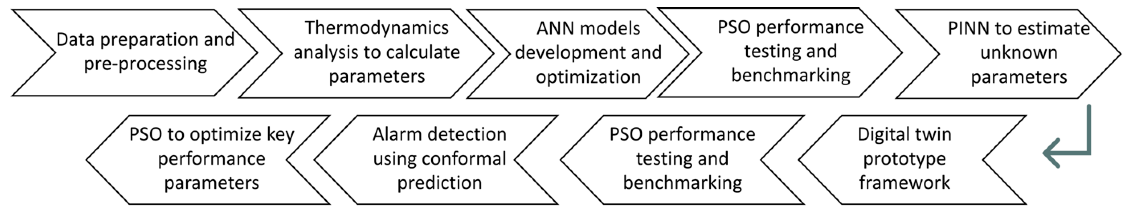
The study started with data preparation and pre-processing, as illustrated in Figure 1. Next, the identified critical parameters are generated using thermodynamic analysis under a steady state and ideal gas assumption. This process includes collecting data from the original equipment manufacturer (OEM) of M701F and making assumptions for constant properties. After that, feature selection was conducted to develop the three ANN models whose performance was then evaluated by using R2 score and mean squared error. The performance of the ANN model was compared with three different machine learning algorithms: linear regression (LR), support vector regression (SVR), and XGBoost.
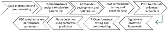
Figure 1.
Proposed research framework to develop modeling using thermodynamic analysis and ANN, critical parameter estimation using PINN, testing PSO performance, and optimization using PSO.
Subsequently, PINN was developed to estimate AFR and combustion efficiency (), and the evaluation method to determine the best estimation will be demonstrated. The previously trained ANN models were used in crafting the objective functions to optimize turbine power output (GTPO) and specific fuel consumption (SFC). Prior to this, standard PSO and multiple improved PSO were tested on five distinct test functions, which later were also compared with the benchmark function of Gaussian evolutionary programming (GEP). Suboptimal conditions (alarm) were detected using an inductive conformal prediction. Ultimately, the PSO was used to optimize GTPO and PSO by adjusting controllable parameters.
2.1. Data Preparation and Pre-Processing
Three months of operational data were sourced from a power plant operator. The data were sampled every 3 min from September to November 2023, comprising 202 attributes and 43,720 instances. Many duplicates, irrelevant attributes, and missing values were observed from the raw data, and thus necessitated further data pre-processing.
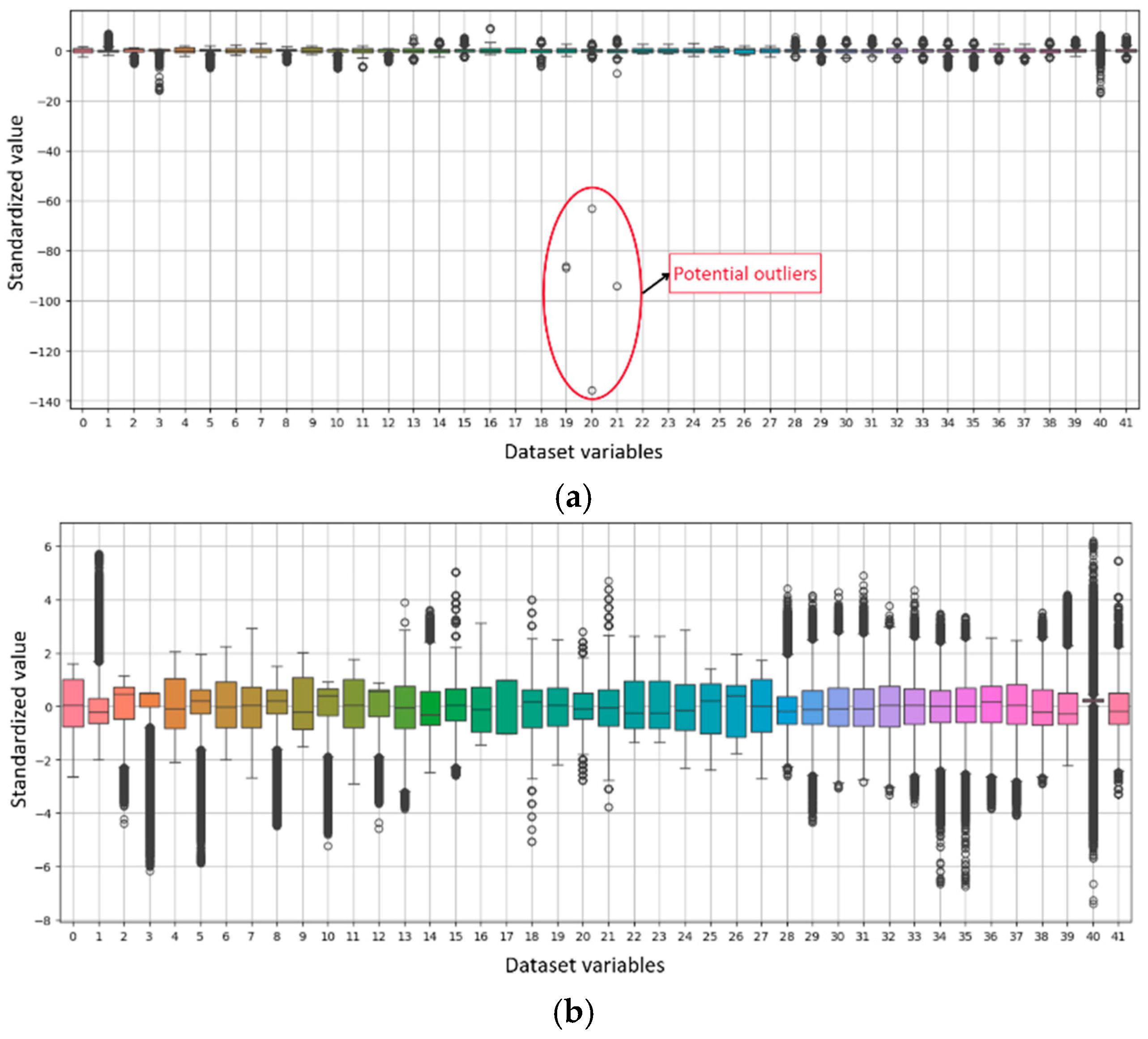
Data pre-processing included removing the least relevant attributes and attributes with significant missing values, and cutting out outliers. The processing of outliers was completed by standardizing the data and discarding datapoints that lie outside the percentile of 0.02 and 0.98. Data standardization is essential to rescale all features into a comparable range and ensure balanced contribution [43]. The standardization uses Z-score normalization with formula , where and refer to mean and standard deviation for a column, while the outlier’s clearance process is visualized in Figure 2.
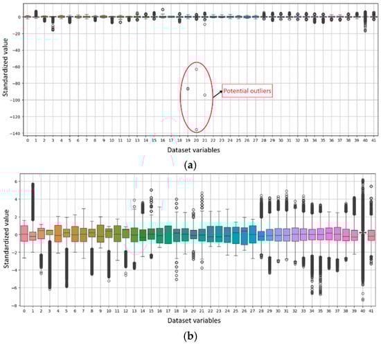
Figure 2.
Processing of outliers visualized in boxplot: (a) before and (b) after outliers’ clearance.
Eventually, the data were reduced into 41 variables and 43,720 instances. A summary of operating parameters in the reduced dataset is depicted in Table 1, and a full summary of available data used to develop the ANN is shown in Table A1.

Table 1.
Summary of operating parameters from real gas turbine operations.
The type of GT used is Mitsubishi M701F, with the configuration and performance specification specified in Table 2. The constant properties, particularly compressor stages and turbine stages, are used in thermodynamic calculation, whereas performance ISO base rating, efficiency, and lower heating value (LHV) provide baseline values to validate the calculation.
Table 2.
Summary of configuration and performance specifications.
2.2. Thermodynamic Analysis
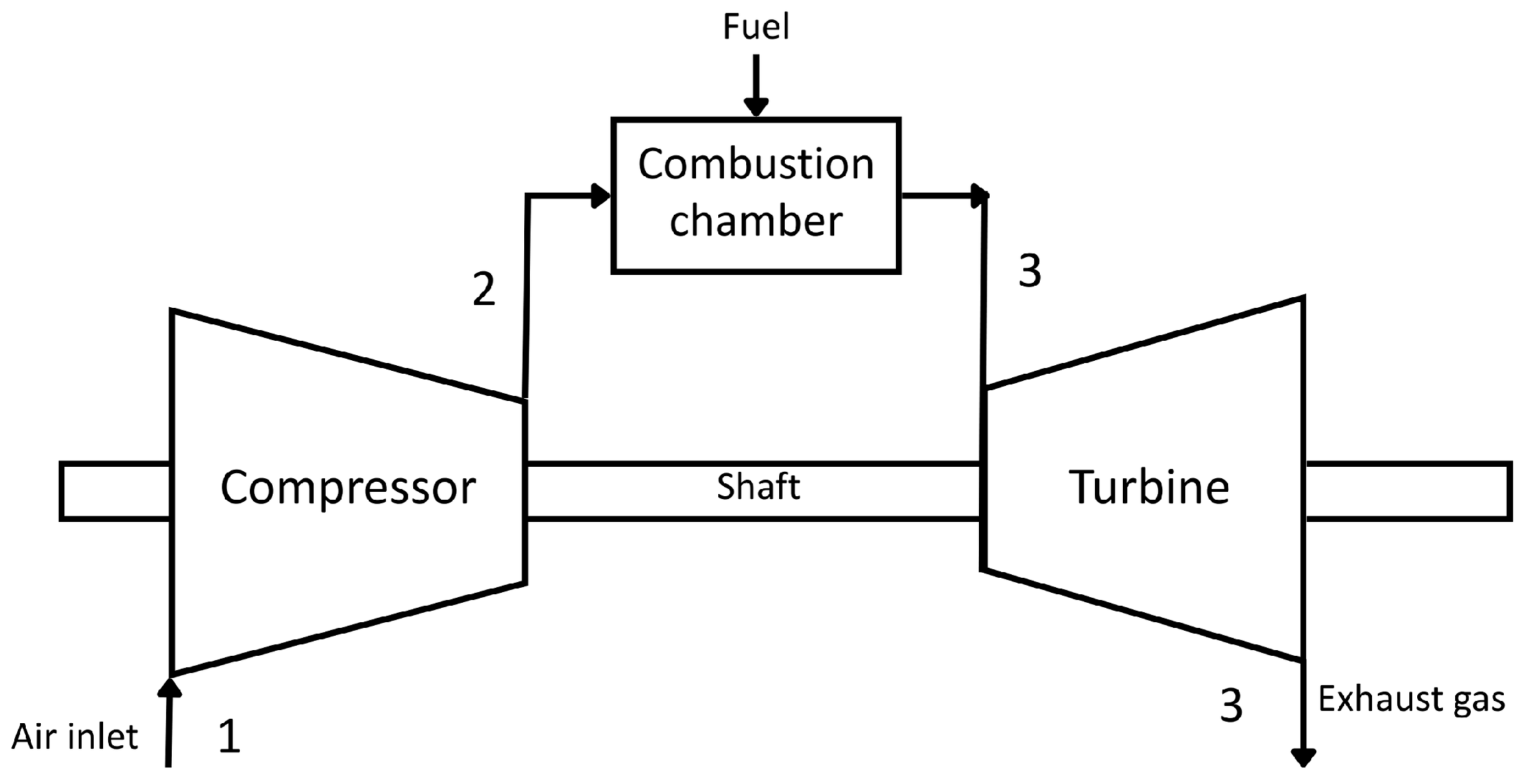
The gas turbine (GT) is modeled with thermodynamic principles following a simple open-cycle GT, as illustrated in Figure 3. The component comprises a compressor, combustion chamber, and turbine. The process scheme is described as follows. Firstly, air is drawn into the compressor to undergo isentropic compression (1–2). The high-pressurized air at the compressor outlet is then mixed with fuel gas in the combustion chamber for ignition (2–3). This results in extremely high-temperature gas at the GT inlet section (3–4). The hot gases are then expanded isentropically across the turbine to be converted into mechanical (rotational) energy, which is used to drive the compressor and the generator shaft. This section highlights how the three components can be modeled using thermodynamics, with a focus on calculating the turbine inlet temperature (TIT) and specific fuel consumption (SFC).
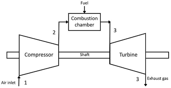
Figure 3.
Schematic of a simple Brayton open-cycle GT.
2.2.1. Compressor Models
Although compressor parameters are beyond the scope of this study, it is still noteworthy to generate any potential baseline parameters that can be useful for overall result validation. Under a steady state and ideal gas assumption, temperature at the compressor outlet, , can be expressed with the following equation:
with ambient temperature °C, pressure ratio from OEM data, specific heat ratio of air [27], and compressor isentropic efficiency assumed from [28]. Next, work completed by compressor, , is given by the following:
with as compressor mechanical efficiency and as the specific heat of air that can be either set as a constant or as dynamically varying based on temperature as specified in [27] as follows:
where , valid for . Meanwhile, for gas, specific heat can be expressed by the following.
This study uses simplified cases where the assumed constant values of and are taken from [27].
2.2.2. Combustor Models
The combustion process is modeled as a steady-state exothermic reaction between fuel and air with the assumption of negligible heat loss [44]. The energy balance equation is given by the following.
With the air–fuel ratio (AFR) and the presence of combustion efficiency during the process, the expression can be formulated as follows:
where represents turbine inlet temperature (TIT). Both and lower heating value are provided in the dataset. But, AFR and remain unknown and, hence, will be estimated using PINN, as detailed in Section 2.4. This method would be beneficial for offline monitoring as AFR and are the indicators for combustion performance that are not measuring in the current operation.
2.2.3. Turbine Models
During the isentropic expansion process in the turbine, exhaust gas temperature exiting GT, , can be expressed as follows.
As the exhaust gas temperature is available in the data, then the turbine inlet temperature (TIT = ) can be backcalculated. Pressure ratio is obtained from OEM data, and , as assumed in [27]. As for turbine isentropic efficiency , this is obtained through calculating TIT with varying = [0.75, 0.80, 0.85, 0.90, 0.95] and the rest of the properties as constant. The optimal estimate of is then indicated by the calculated TIT that conforms with the associated TIT range for M701F, which is 1400–1500 °C [45,46].
Furthermore, GT power output (, net work output (), and total GT power () can be defined as follows.
Specific fuel consumption (SFC) also can be expressed as follows.
Total heat input, , of the combustion process is as follows.
Lastly, the turbine thermal efficiency, , and heat rate, , can be calculated as follows.
2.2.4. Constant Properties
Constant properties are necessary for thermodynamic calculation. The properties were taken directly from the relevant literature or taken after experiments whose results were validated by the literature [45,46] shown in Table 3.
Table 3.
Summary of constant properties used.
2.3. Artificial Neural Network (ANN) Modeling
An artificial neural network (ANN) is a computational model inspired by the structure of the brain, which consists of large numbers of interconnected neurons that process information through weighted connections [47]. It is a universal function approximator that can model complex nonlinear relationships between inputs and outputs [33]. It consists of multiple layers that transform the input features progressively using neurons (weights and biases). An ANN type of feed-forward neural network is used in this study, as illustrated in Figure 4.
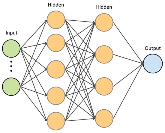
Figure 4.
Illustration of fully connected feed-forward neural network architecture.
Three ANN models are crafted to predict TIT, SFC, and GTPO separately. Generally, the modeling started with feature selection to choose the most relevant features to predict a certain output. The ANN is then trained and optimized using random search and PSO. Ultimately, the performance of the optimized ANN models will be compared with three machine learning algorithms including linear regression (LR), support vector regression (SVR), and extreme gradient boosting (XGBoost).
2.3.1. Feature Selection
Too many features used in the input layers of ANN may overcomplicate the model in discovering the data patterns to predict a particular output. Therefore, feature selection is crucial to enhance model performance and reduce redundancies among the features. The following three steps were implemented: (1) mutual information analysis to quantify dependencies between each feature and the target variable; (2) variance inflation factor (VIF) to identify the degree of multicollinearities that may reduce model performance (features with VIF > 5 were iteratively discarded until all features showed a VIF below 5); and (3) Pearson correlation analysis to eliminate features with a low correlation with the target.
2.3.2. Data Splitting
Before training the ANN, the dataset was firstly divided into training, validation, and testing sets. Chronological splitting was applied to preserve temporal dependencies in the time-series data. Among the three months of data, October data were used for training (), November for validation (), and September for testing (). This approach ensures that the ANN generalizes across different monthly operating regimes.
2.3.3. ANN Model Setup
Given an input , the ANN model with number of hidden layers transforms the input recursively using expression as follows:
where and represents weight matrix and bias vector of layer , respectively. The variable denotes the input to the -th layer, with referring to its corresponding output. The activation function is applied at layer . After passing through hidden layers, the final output of the ANN model is denoted as . A set of hyperparameters may include a number of hidden layers, an activation function for each layer, optimizers, and a dropout ratio.
Optimizers refer to gradient-based optimization algorithms used to update trainable parameters (i.e., weights and biases) for each training loop. The update is based on computed gradients from backpropagation algorithms. Stochastic Gradient Descents (SGC) and Adaptive Momentum (ADAM) [48] are considered in this paper.
2.3.4. ANN Model Training and Validation
The objective of training an ANN is to minimize a loss function with mean squared error () given by the following:
where denotes ANN prediction output at -th sample and refers to its corresponding true value, with as number of training samples. Before training the parameters, Glorot Uniform [49] is used to initialize trainable parameters ( in the network to reduce the risk of vanishing or exploding gradient problems. After training iteration is completed, the final optimal that minimizes is obtained.
The trained model is then validated using the validation set to see the model generalization. A well-generalized model (proper fit) indicates a well-performing model on an unseen dataset (testing set). Poor generalization can be caused by overfitting and underfitting during training and validation processes. Overfitting describes a model that overly memorizes the training data such that it struggles with unseen data, while underfitting reflects an inadequate learning capability. They can be observed by plotting both true values and predicted values on a time-series plot, or by plotting loss convergence over the epochs, with an epoch defined as one complete training pass. To prevent overfitting, an early stopping mechanism is applied by halting the training when validation loss stops improving for a pre-defined consecutive epoch, known as the patience value. Additionally, tuning the patience value can further enhance overall model performance and generalization [50].
2.3.5. ANN Hyperparameter Tuning
There are various methods to fine-tune ANN hyperparameters, and this study explores the use of random search and PSO. Five different hyperparameters are to be tuned, including learning rate, dropout ratio, number of nodes per layer, activation function per layer, and optimizer. The search spaces are depicted in Table 4.
Table 4.
Summary of search space used for ANN optimization.
With random search, multiple sets of hyperparameters were formed based on values randomly selected using uniform distribution from the search space. ANN performance for each set of hyperparameters is evaluated to select one that gives best performance and generalization.
Subsequently, PSO is implemented to optimize (fine-tune) the ANN by encoding the hyperparameters into particles. Each particle is represented as a numerical vector given by the following:
with as the learning rate, as the encoded optimizer, and as the number of nodes, activation function, and dropout ratio in layer for hidden layers. The position and velocity vectors () for the particles are then initialized using uniform distribution from the search space, with as the number of populations, as the number of hyperparameters embedded in each particle, and as the total number of particles per population. The fitness function () for particle in population is evaluated from the ANN validation loss . The position and velocity of each particle is then updated for each iteration, and the global position at the last iteration is determined as the most optimal hyperparameters. More about PSO will be discussed in Section 2.5.
2.4. PINN to Estimate AFR and Combustion Efficiency ()
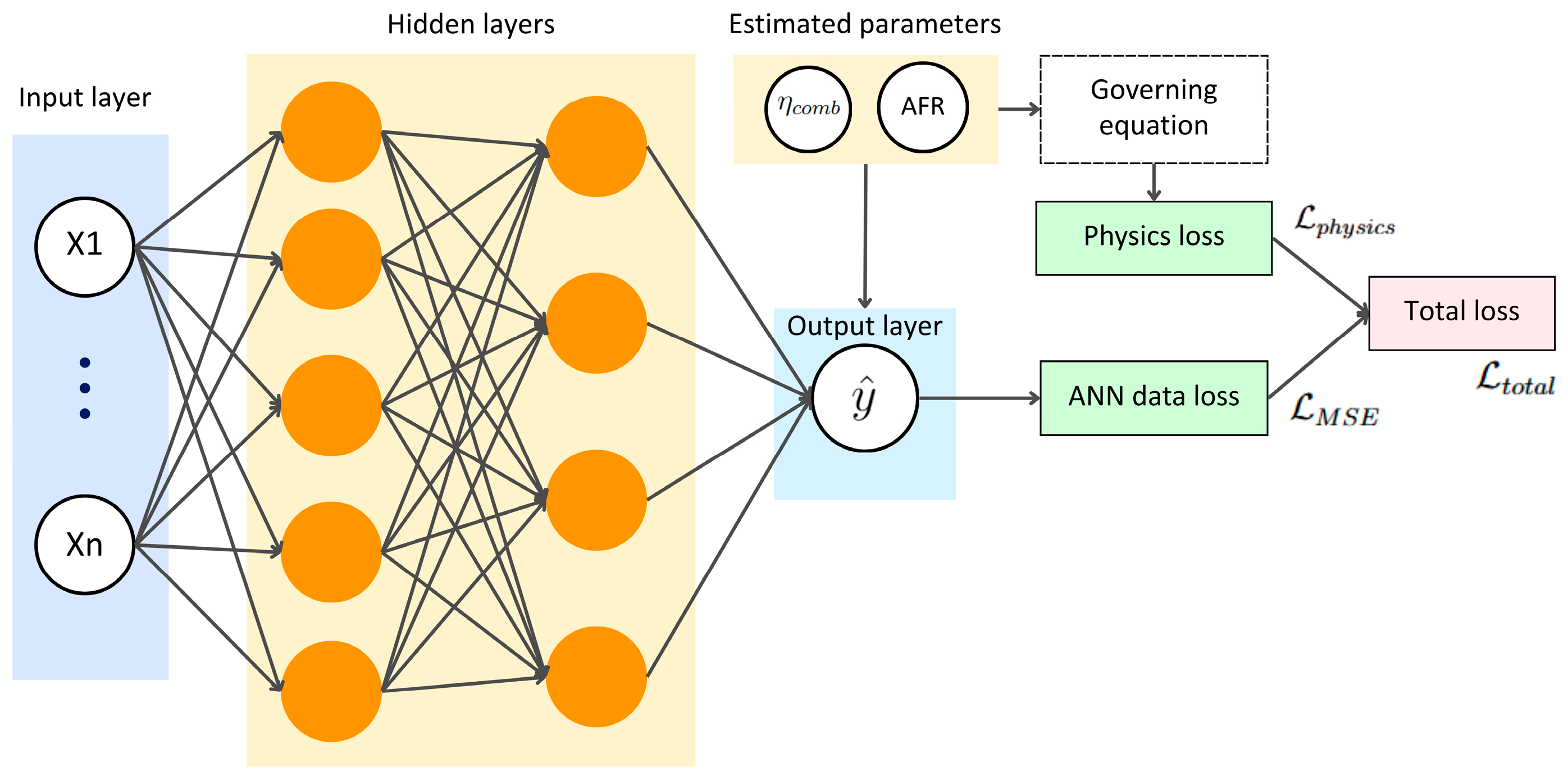
To estimate both parameters of air–fuel ratio (AFR) and combustion efficiency (), the following TIT governing equation from the energy balance equation during the combustion process is used as physics loss, which is expressed as follows:
where and are temperature at compressor outlet and turbine inlet from data index , respectively. AFR and combustion efficiency for each time index are set as trainable parameters. This physics loss function is then averaged with data loss from mean squared error (), forming the total loss function, expressed as follows:
with as weightage proportion of physics loss.
The training strategy is built upon the framework illustrated in Figure 5. The ANN model to predict TIT that had been previously optimized was used to make the prediction. But, for this case, additional trainable parameters consisting of AFR and are added with initial conditions (ICs). Boundary conditions (BCs) for both parameters are also defined as 15–55 for AFR and 0.95–1 for . ICs for AFR are set for five different values of [15, 20, 25, 30, 35], whereas ICs for and are, respectively, set to 1 and 0.5. The rationale of multiple ICs for AFR is to explore a wider range of possible solutions of AFR.
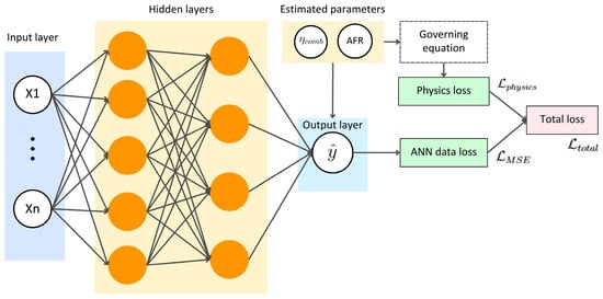
Figure 5.
PINN training diagram to estimate AFR and using TIT ANN model.
Subsequently, the dataset is split into training and testing sets. During the training process, physics weight is also attached as an extra trainable parameter. Once optimal is obtained, it is then detached from the trainable parameters and used as a constant value to estimate AFR and in the testing set. At the end of the estimation, five different possible solutions are be evaluated based on the total loss and the conformance with the BCs.
2.5. Particle Swarm Optimization (PSO) Algorithm
2.5.1. PSO Overview
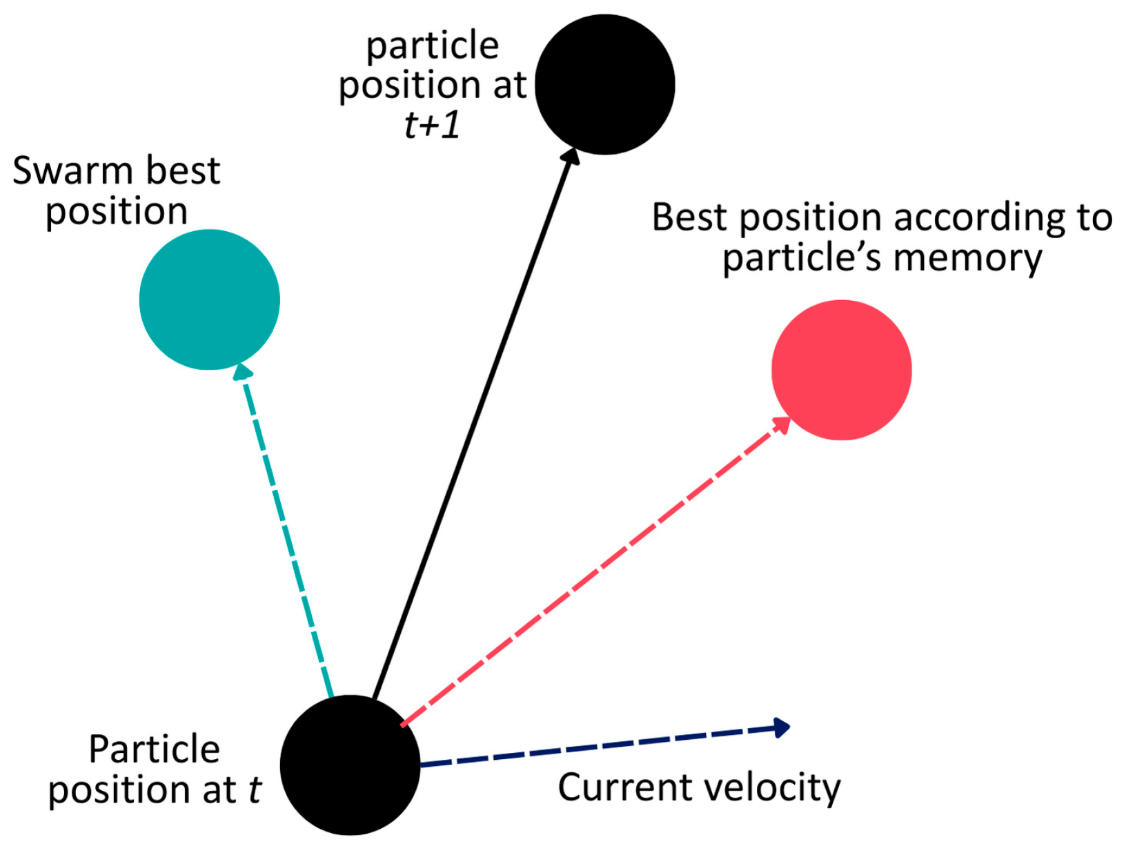
Inspired by bird flocking or fish schooling, PSO works by distributing particles into n-dimensional search space to search for the best position that minimizes or maximizes the fitness function. When searching for the best position, particle movement is influenced by three main factors, as illustrated in Figure 6, namely the current velocity of the particle itself (inertia), the particle memory of its best historical position (cognitive), and the best position according to the swarm (social).
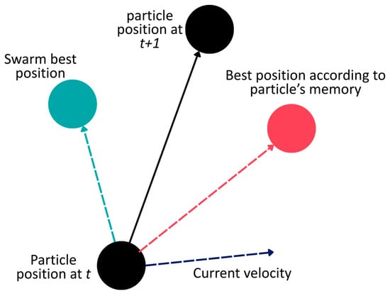
Figure 6.
Particle’s position update mechanism from iteration to .
In the most basic form of PSO, the mechanism to update the particle’s position and velocity from iteration to can be written as follows:
where represents th particle among particles in a population. and are the position and velocity of th particle with dimension. refers to th particle’s historical best position from its memory, while denotes the global position of the population. and are two independent random numbers within the range of (0, 1), while and define the iterations.
PSO parameters including inertia weight , cognitive learning factor , and social learning factor are also important as they highly affect PSO performance and, hence, they must be tuned. As for inertia weight, lower tends to make the particles converge faster towards global best, while higher influences particles to exploit new search areas and converge with a slower rate. Shi and Eberhart [51] introduced optimal inertia weight within [0.9, 1.2] and suggested that linearly time-decreasing can significantly improve the performance. In this study, constant inertia weight is used and the selection of optimal inertia weight is beyond the scope of this study. Subsequently, the value for learning factors and of 2.8 and 1.3 are taken based on Carlise et al.’s [52] demonstration after rigorous experiments.
Further, this study also considers multiple population or swarm PSO to co-exist in the search space. Best fitness functions among the population are then evaluated to select the most optimal position.
2.5.2. Improved PSO
In this study, the standard PSO algorithm is enhanced to improve its global search capability, avoid premature convergence, escape local optima, and prevent excessive mutation. Inspired by recent PSO advancements discussed in [38,41], this study proposes an improved PSO with Gaussian jumps and controlled mutation (IPSO + GJ + CM), with a complete framework demonstrated in Figure 7.
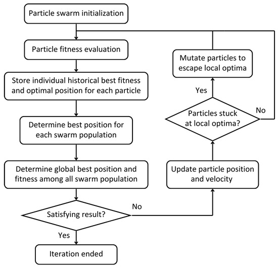
Figure 7.
Flowchart of the proposed IPSO + GJ + CM.
The additional features consist of Gaussian jumps and controllable mutation. With the base of standard PSO discussed in the earlier section, any particles showing stagnation or non-improving fitness consecutively for a threshold of maximum_number_failure will be indicated as stuck at the local optima, and, hence, must be mutated by Gaussian jumps written as follows:
where the term is used to perturb the particle’s position, with as a scaling factor and as a random factor sampled from Gaussian distribution. The perturbance will allow for the particle to escape from local optima, therefore allowing wider exploration. During the iteration, if the number_of_failure or the number of mutations exhibited by a particle reaches maximum_number_mutation, the particle then stabilizes with zero velocity to prevent endless jumps, restricting excessive mutations that result in over-randomization.
2.5.3. PSO Testing and Benchmarking
To measure the performance of the proposed IPSO, it is then compared with 9 other PSO variants. The PSO variants were derived from the two PSO bases, namely IPSO, which adopts standard PSO as its base, and Gaussian PSO (GPSO) that excludes inertia weight in the velocity formula, as proposed in [53]. Both Gaussian and adaptive Cauchy jumps [41] are applied to both IPSO and GPSO. Similarly, controlled mutation (CM) is also implemented to check whether it improves PSO with jumps. Additionally, PSO with constriction factor (KPSO) proposed in [54] is also included. As such, the PSO variants can be expanded, as summarized in Table 5.
Table 5.
Summary of 10 PSO variants tested in this study, with IPSO + GJ + CM as the proposed improved PSO.
The 10 PSO variants are subsequently tested on 5 popular test functions as depicted in Table 6. Each function has their own characteristics. For instances, Schwefel function () is highly multimodal with many local optima with global minimum located near its boundary of the search space. Rastrigin function () is highly multimodal with a regular grid of local minima. Ackley function () combines exponential term with cosine term, creating a nearly flat outer region and a sharp peak at global minimum, testing the algorithm’s balance in exploration and exploitation due to its shallow gradient and multimodal nature. Griewank function () has many local optima and is relatively easier to find due to its moderate multimodality. Lastly, penalized function () introduces penalty terms, creating a complex and discontinuous landscape with sharp boundaries. In addition, the performance of IPSO + GJ + CM is benchmarked with Gaussian evolutionary programming (GEP) taken from [55]. Next, IPSO + GJ + CM is used to fine tune the ANN model in this study for optimization and is also used for GT performance optimization in the digital twin framework.
Table 6.
Five benchmark test functions with many local optima used for performance comparison in this study, with as number of dimensions (), as lower and upper boundary of the search space, and as global minimum value of respective function.
2.6. Alarm Detection Using Conformal Prediction
Instead of using a traditional statistical tool like moving average or weighted moving average, prediction interval is used to generate the alarms. Inductive conformal prediction (ICP) can produce a prediction interval at a given confidence level (i.e., 95% and 80%) by measuring non-conformity scores . The score is computed using a calibration set after the model is fitted using the training set. After that, the prediction interval for a new prediction set of can be symmetrically given by .
The region within the prediction interval is deemed as an optimal region, such that any true values lying outside the interval will trigger alarm. In the context of gas turbine power output (GTPO), the region above the prediction interval is considered suboptimal due to its negative magnitudes, implying work completed by the turbine on its surroundings, while regions below the prediction interval are retained as acceptable due to their high magnitudes. Additionally, the operational regime of off-peak load hours was excluded in the alarm.
2.7. IPSO + GJ + CM and ANN Models to Optimize GT Performance
Two different optimization tasks are created in this study: (1) optimize GT power output by adjusting AFR and (2) optimize specific fuel consumption (SFC) by adjusting AFR and IGV position. The optimization is processed for each time index in the performance metrics where the suboptimal condition has been previously detected using conformal prediction. The previously optimized ANN models are then integrated to predict the output given adjustable controllable parameters. The objective function to optimize GTPO is given by the following:
where represents the GTPO ANN model and refers to the input features required for . PSO particles are set up to find the optimal value of AFR, which is also included in . The boundary for the controllable parameters is defined as , where and are the mean and standard deviation of corresponding controllable parameters from the operational data. As for SFC optimization, a similar objective function is also set up with PSO optimizing both AFR and IGV position independently.
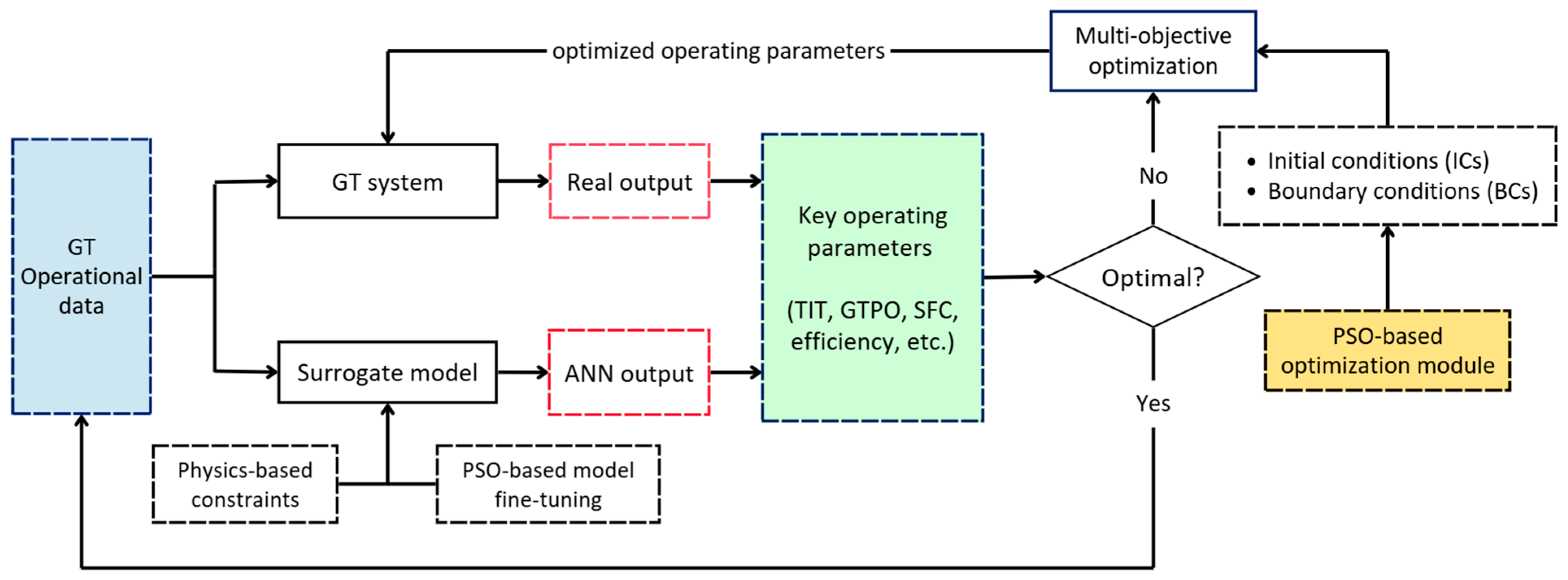
2.8. Digital Twin Prototype (DTP) Framework for Gas Turbine
The final effort to optimize GTPO can be described in the framework illustrated in Figure 8. It forms a closed loop where the optimized controllable parameters are fed back to the physical system.
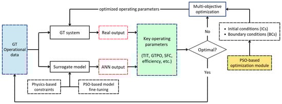
Figure 8.
The proposed closed-loop optimization framework to optimize GTPO and SFC.
2.9. Resources Used for Experimentation
The computational tasks in this study—ANN, PINN, and PSO—were primarily executed using a local GPU workstation with CUDA 12.6 [56] in a laptop with NVIDIA GeForce RTX 3060, 32 GB RAM, and a 64-bit operating system, whereas the software used includes Python 3.8.20 [57], Anaconda 24.9.2 [58], and Jupyter Notebook 7.3.2 [59].
3. Results and Discussion
The results are organized as follow: (1) results on critical parameter calculation using thermodynamic analysis; (2) AFR and combustion efficiency estimation using PINN; (3) ANN model development; (4) PSO benchmarking result; and (5) optimization result.
3.1. Results on Parameter Calculation Using Thermodynamic Analysis
Several essential parameters including TIT, LHV, GT thermal efficiency (), and SFC were calculated from the operational data and constant properties, as depicted in Table 7. The results show that the TIT mean value is 1464.24 °C, aligned with OEM data where TIT for typical GT lies around 1400–1500 °C [45]. Thermal efficiency shows 31.34%, 10% lower than the design value of 41.9%. SFC calculation is validated with the calculated SFC of 0.46 to 0.50 kg/kWh in [60] for M701F. Eventually, the calculated TIT and SFC will be used as a data label to develop ANN models.
Table 7.
Summary of calculated parameters using thermodynamic analysis.
3.2. Results of ANN Modeling
3.2.1. ANN Model Optimization
Table 8 shows the final ANN models for TIT, GTPO, and SFC that have been optimized. TIT and GTPO shows lower scores of 94.03% and 82.27%, while SFC indicates a significantly higher score of 97.59%. This may be due to different complexities in predicting the three outputs. GTPO exhibits the characteristic of a discrete signal, which makes it more difficult to predict, while TIT and SFC have the continuous form of a signal. The different composition of input features may also contribute to the accuracy of the model. Given the results, the TIT model is then used for PINN, while both GTPO and SFC are utilized for GT optimization.
Table 8.
Summary of three final optimized ANN models.
Prior to the final optimized models, model optimization is run for a varying number of hidden layers for each model as depicted in Table 9. The optimization was carried out using PSO and random search (RS). PSO were initialized with 30 particles, 5 populations, and 150 iterations. This implies that 150 sets were initialized, all of which may change for 150 couple times. Meanwhile, random search generates 2000 sets of hyperparameters. The results demonstrated that PSO can compete against RS. The score achieved by RS is slightly higher than PSO for TIT and GTPO models, while for SFC models, RS yielded significantly poor results compared to PSO. Moreover, the PSO takes a relatively larger amount of time but significantly lower memory compared to RS.
Table 9.
ANN model optimization using IPSO + GJ + CM and random search for each of the hidden layers of TIT, GTPO, and SFC models.
It is also observed that model accuracy tends to decrease as the number of hidden layers increases. When the model architecture becomes more complex, but the training data remain limited, this may lead to overfitting, inefficient training, and unstable learning.
3.2.2. ANN Models Compared to Machine Learning Algorithms
The previously optimized ANN models were also compared with three ML algorithms in terms of score. The results in Table 10 show that ANN significantly outperforms them for TIT and GTPO models but is competitive for the SFC model. One of the possible reasons could be that TIT and GTPO have relatively more complex data representation, making it more difficult for ML algorithms to handle. However, SFC has less noisy and less complex data such that ML algorithms can learn sufficiently. This shows that simpler ML algorithms could perform better than a complex ANN model in some applications, which could potentially save computational cost in online/offline applications.
Table 10.
Summary of ANN model performance compared with three machine algorithms: linear regression (LR), support vector regression (SVR), and XGBoost.
3.3. Results of AFR and Combustion Efficiency Estimation Using PINN
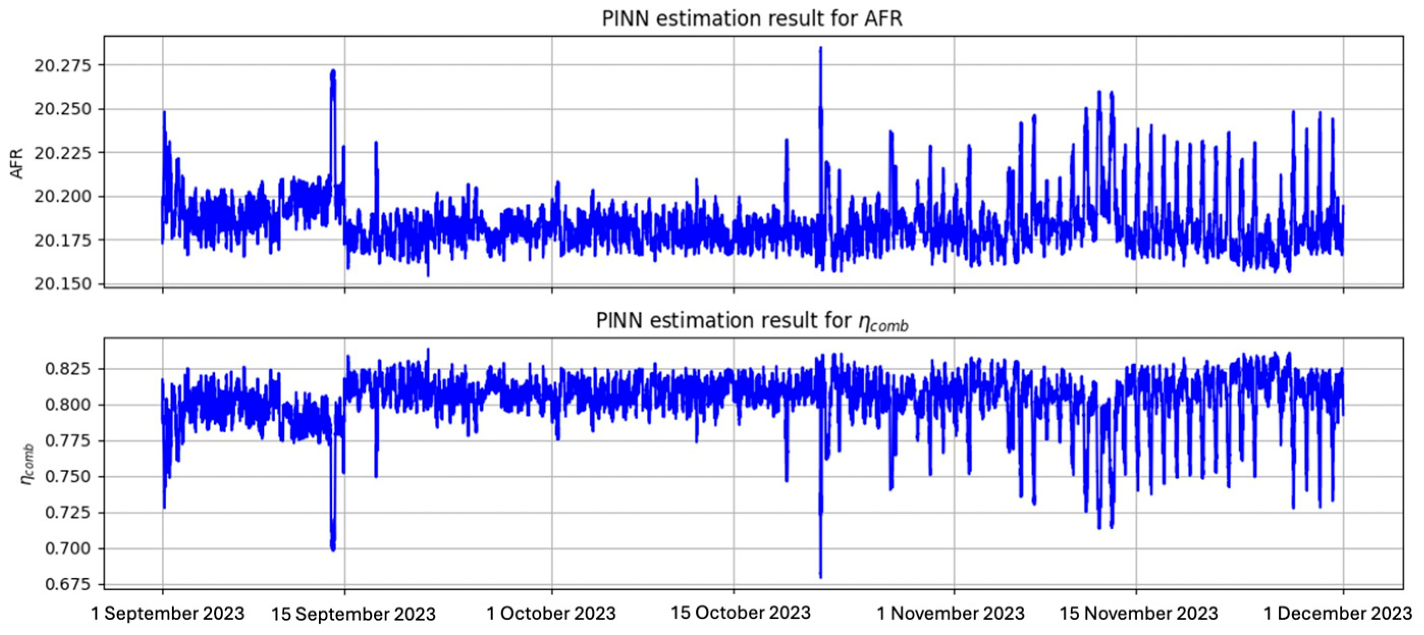
Multiple initial conditions (ICs) of AFR were evaluated to select the best PINN estimation result. As summarized in Table 11, an initial AFR of 25 that generates a final AFR of 25.016 and of 0.983 with the lowest total loss of 0.105 was selected as the best solution. The options with initial AFR values of 15 and 20 are considered acceptable but were not selected due to higher losses. The rest were rejected because the final is outside the pre-defined boundary conditions (BCs) of 0.95 to 1. The final solution of AFR has a mean value of 25.016, standard deviation of 0.021, and range of [24.974, 25.259]. Meanwhile, that of has a mean value of 0.984, standard deviation of 0.022, and range of [0.832, 1.026]. This is consistent with the calculated AFR of 20–35 and of 0.95–1.00 as reported in [60,61,62]. However, a small number of indices that output values above 1 were still observed in the final solution, indicating the violation of BCs. These were potentially caused by the underlying noises and biases preserved in the data. As for an alternative solution, the option of a final solution of and was also considered as an acceptable solution despite the lower AFR and values.
Table 11.
Summary of PINN estimation result after 3000 iterations for multiple initial AFR.
Figure 9 describes the correlation of both dynamic parameters (AFR and ) for the option with initial from Table 11, which exhibits a negative correlation of −0.98 as hypothesized. PINN demonstrated success in estimating AFR and for each time index. This outcome is further validated by plotting AFR against thermal efficiency, as depicted in Figure 10; it is then compared with a similar plot in [27]. The result shows similar correlation, in which thermal efficiency and TIT are reduced when AFR is increased. It is also noteworthy to observe how a small reduction in AFR can lead to significantly higher thermal efficiency.
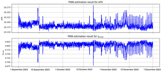
Figure 9.
Best PINN estimation solution of AFR and visualized in time-series plot.
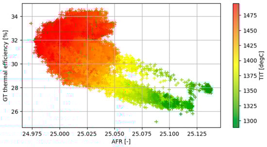
Figure 10.
Scatter plot of the PINN-based estimated AFR vs. thermal efficiency with TIT.
Despite the success of PINN to estimate unknown parameters in a governing equation, its limitation must also be noted. Firstly, proper initial conditions must be selected as their incorrect selection may make the PINN diverge easily; therefore, the domain knowledge about the parameter must be carefully considered. Secondly, the sensitivity of the final estimated parameters may be highly affected by vanishing or exploding gradients, such that it must be well mitigated.
3.4. Results of PSO Algorithm Benchmarking
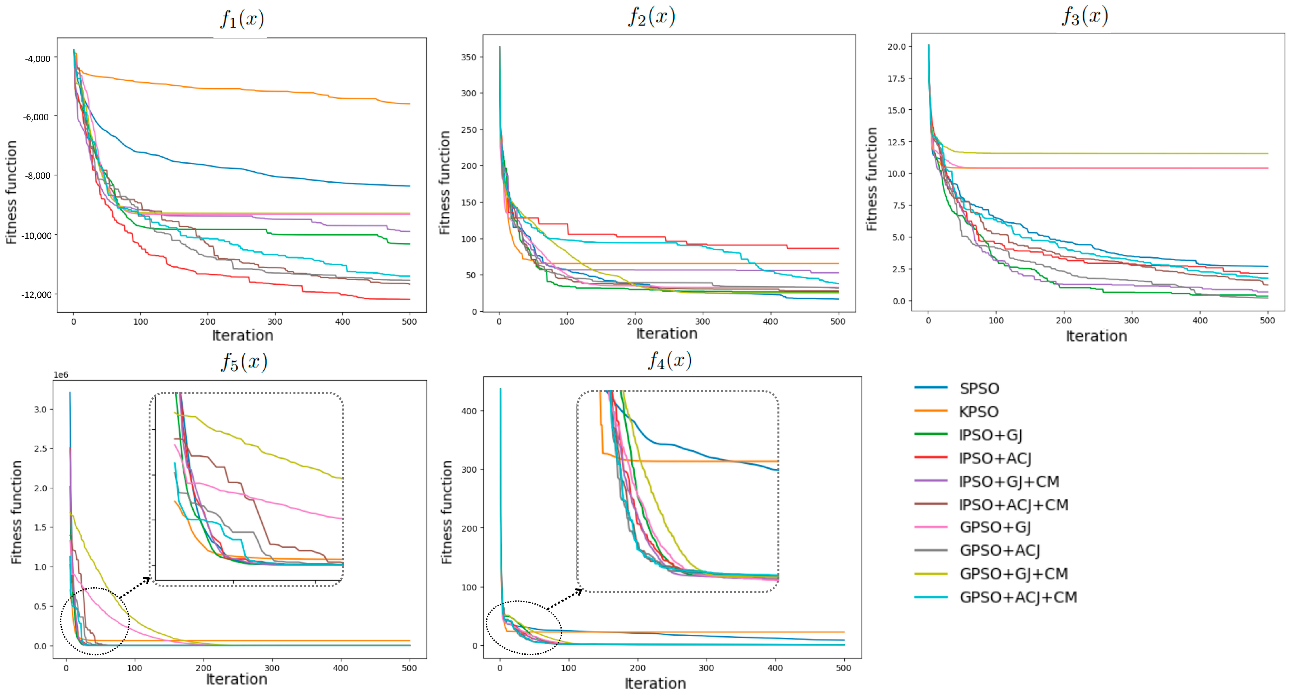
Initialized with similar particles, 10 PSO variants were run to minimize five test functions with 500 iterations. They were then compared to each other and benchmarked with GEP taken from [55]. As summarized in Table 12, although the proposed IPSO + GJ + CM did not perform as the best variant across all functions, it generally outperformed the GEP (except for ). It is also inferred that adopting the jumps strategy significantly improved standard PSO. The implementation of controlled mutation did not improve the PSO, but generally reduced the memory consumed during iterations. Although IPSO + GJ + CM was not the best model amongst the tested PSO variants, it remains used in this study.
Table 12.
Performance summary of 10 PSO variants over 500 iterations, with as the mean loss at the end iteration and as standard deviation of fitness value throughout the whole iteration.
The improvement of all PSO across five test functions is further visualized in Figure 11, where it describes the progression of fitness function over iterations. The varying performances observed may be caused by distinct characteristics exhibited by each test function.
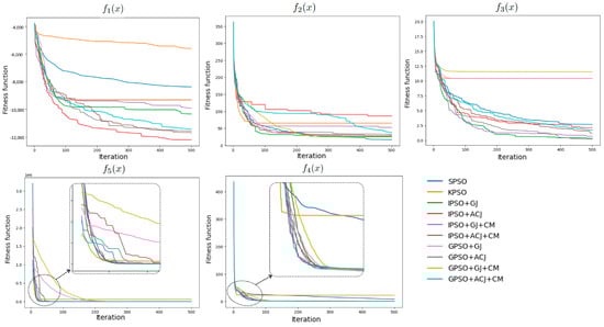
Figure 11.
PSO convergence for 10 different variants over 500 iterations, where PSO parameters are set at w = 0.8, c1 = 2.8, c2 = 1.3, 50 particles, 100 populations.
3.5. Results of GT Performance Optimization
This section demonstrates the results of the detected suboptimal conditions (alarms) by conformal prediction and how PSO managed to optimize the operating parameters.
3.5.1. Results of GTPO Optimization
Given a confidence level of 95%, the prediction interval indicated by the blue-shaded region in Figure 12 is generated. Any true values that lie above this interval and occur within peak hours are distinguished as suboptimal or alarming conditions. In total, 1063 reduced alarms were detected across the September dataset. The alarms show that a sudden increase in the magnitude of GTPO indicates increased power demand and operational stresses. This behavior is possibly linked to AFR imbalance during the load fluctuation and transition. The daily repetitive pattern also suggested a strong association with the GT operating cycle rather than random anomalies.
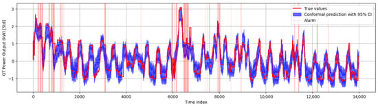
Figure 12.
Detected alarms in September 2023 based on conformal prediction with GTPO model.
A shorter time window on 1 September 2023 was selected to be optimized. Figure 13 demonstrates successful optimization such that the non-optimal true values in the red-shaded region (alarms) were recovered back into the prediction interval, leading to a significant increase in GTPO. Despite the success, several limitations were identified. Firstly, it took almost 27 h to complete the optimization process of this small time window, making such runtime less ideal for real-time use. Secondly, the GTPO is optimized with the assumption of dynamic control in AFR. This can be addressed by developing a proper experiment setup to ensure the reliability and validity of dynamic control in AFR.
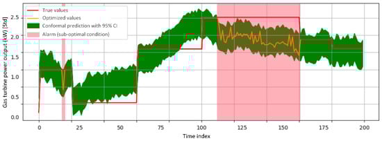
Figure 13.
Results of GTPO optimization on a shorter time window of the alarmed condition.
3.5.2. Results of SFC Optimization
Efforts to optimize SFC using a similar approach to GTPO was also attempted. For this case, two controllable parameters—AFR and IGV positions—are considered as decision variables. When SFC exceeded a predefined setpoint under normal load, PSO was triggered to adjust both parameters independently to minimize fuel usage.
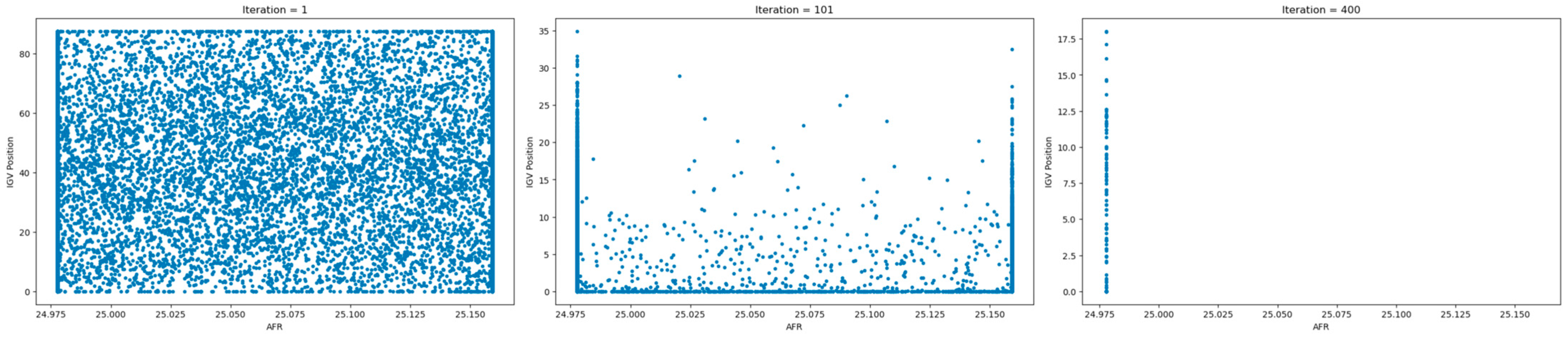
Figure 14 illustrates particle movement across 400 iterations. Initially (iteration 1), particles are uniformly distributed across the two-dimensional search space. By iteration 101, IGV values begin collapsing toward the lower limit, while AFR clusters near the upper bound. At iteration 400, particles converge sharply at boundary extremes, indicating PSO has over-optimized both variables. Although this managed to reduce SFC, the solution was impractical. The final optimized AFR remained static, while IGV was minimized without proper measures on the system behavior. The core issue may be caused by the overly simplified objective and weak penalty functions, ignoring critical dependencies among the two parameters.
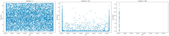
Figure 14.
The movement of particles representing two independent controllable parameters adjusted by PSO at iteration 1, 101, and 400 to optimize SFC.
4. Conclusions
This study proposed a modular digital twin prototype framework integrating thermodynamic modeling, ANN for data-driven prediction, PINN, and performance optimization using PSO, all of which is clustered into sub-modules: modeling, estimation, and optimization. Thermodynamic modeling was utilized to calculate TIT, SFC, and other relevant performance metrics using available data. The developed ANN for TIT, SFC, and GTPO showcased strong performance with scores of 94.03%, 82.27%, and 97.59%, respectively, after being optimized via PSO and random search. It is observed that the performance of PSO and random search were on par, and the general performance of ANN outperformed that of some machine learning algorithms (i.e, linear regression, XGBoost, and SVR). Several challenges added more complexity to the modeling module. Firstly, the unavailability of data led to many identified missing parameters. Secondly, the insufficient data and the selection of ANN architecture that was relatively considered shallow or simple significantly affected the performance of ANN models.
Moreover, the thermodynamic and ANN models—to predict TIT—were combined to construct PINN, which successfully estimated the values of AFR and dynamically. The results also conform with the values taken from the literature for a similar type of GT. Despite the conformalities, the calculated parameters may not correctly represent the true values in the GT operations due to other factors such as reliability and unidentified losses, necessitating extended validation by the operator or dataset provider. The PINN estimation of AFR and required extensive manual tuning due to its sensitiveness towards pre-defined initial conditions that is highly dependent on expert knowledge. A similar approach to estimate parameters in a partial differential equation may not be suitable.
As for the optimization module, a PSO variant of IPSO + GJ + CM was tested among different PSO variants. Not a single PSO variant was universally optimal, but the proposed IPSO performed better when compared to GEP as the benchmark algorithm. The IPSO was then employed to maximize GTPO and minimize SFC separately under real-time use cases, with the objective function crafted by leveraging ANN models. Despite the optimization achieved, the control parameters exhibiting the lack of dynamic controls and constraints still become significant limiting factors. The heavy computational memory and runtime consumed also posed challenges to create a reliable optimization for real-world implementation.
Prior to optimization, the alarm detection was built upon conformal prediction intervals during normal GT loading. The advantage of this method is that it may dynamically indicate alarms or sub-optimal conditions during significant operational transitions rather than relying on static upper or lower control limits. Further validation using maintenance logs from the operator would strengthen these findings.
For future development, expanding the framework to include compressor parameters and transient condition analysis would address the current scope limitations. Due to GT data’s limited availability, further GT modeling using process software may also be considered to provide additional baseline data. Subsequently, data-driven modeling can be carried out using more deep learning algorithms to capture more complexities. PINN’s application may be extended to investigate transient conditions involving partial different equations to further leverage its automatic differentiation capability. Deep reinforcement learning may also address the challenges related to the dynamic controls and constraints posed in the real-time optimization task carried out in this study. As performance optimization for real-time cases may be reliably challenging, more focus on higher-level cases towards operational efficiency and fuel cost savings through SFC optimization can be emphasized to significantly impact and benefit the operator. Ultimately, a more holistic closed-loop digital twin prototype framework consisting of multiple integrated modules can be developed to support a more practical implementation for GT operations.
Author Contributions
Conceptualization, methodology, software, investigations, data curation, validation, formal analysis, J.T.L. and A.H.; resources, writing—review and editing, J.T.L. and E.Y.K.N.; writing—original draft preparation, visualization, A.H.; conceptualization, supervision, project administration, E.Y.K.N.; project administration, J.T.L. All authors have read and agreed to the published version of the manuscript.
Funding
This research received no external funding.
Data Availability Statement
The data presented in this study are available on request from the corresponding author. The data are not publicly available due to confidentiality restrictions.
Acknowledgments
The authors would like to first express their gratitude to Nanyang Technological University (NTU), Singapore, and the local power operator in Singapore for the opportunity to study this topic. The corresponding authors would also like to extend their sincere appreciation to other co-authors for their support.
Conflicts of Interest
The authors declare no conflicts of interest.
Appendix A
The operational data attributes extracted from a power plant operator.
Table A1.
Summary of description of the extracted operational data.
Table A1.
Summary of description of the extracted operational data.
| Variable Name | Variable Long Name | Unit |
|---|---|---|
| ACTLD | Actual load | MW |
| BPT | Blade path temperature | °C |
| BPREF | Baseline pressure reference | kPa |
| CSP | Combustor shell pressure | bar |
| COT | Compressor outlet air temperature | °C |
| CIT | Compressor inlet air temperature | °C |
| DE | Differential expansion between turbine and casing | mm |
| TOT | Exhaust gas average temperature | °C |
| FGF | Fuel gas flow | kg/s |
| FGHT | Fuel gas heater outlet temperature | °C |
| FGSP | Fuel gas supply pressure | kPa |
| FGT | Fuel gas temperature | °C |
| CompEff | GT compressor efficiency | - |
| GTPL | Estimated GT Part Loading | µm |
| GTPO | GT power output | kW |
| GPF | Generator power factor | - |
| GTGO | GT generated output | kW |
| Speed | GT Speed | RPM |
| HPCV | HP control valve | - |
| HPSV | HP stop valve | - |
| ICV | Inlet control valve position | - |
| IGV | Inlet guide vanes position | - |
| IGVCSO | Inlet guide vanes closed shut-off | - |
| IFDP | Inlet air filter differential pressure | kPa |
| IMSP | Inlet manifold static pressure | kPa |
| IPCV | Intermediate pressure bypass control valve | - |
| LPBT | LP last stage stationary blade temperature | °C |
| Gb1X | Gearbox bearing 1 X-vibration | µm |
| Gb1Y | Gearbox bearing 1 Y-vibration | µm |
| Gb2X | Gearbox bearing 2 X-vibration | µm |
| Gb2Y | Gearbox bearing 2 Y-vibration | µm |
| Gb3X | Gearbox bearing 3 X-vibration | µm |
| Gb3Y | Gearbox bearing 3 Y-vibration | µm |
| Gb4X | Gearbox bearing 4 X-vibration | µm |
| Gb4Y | Gearbox bearing 4 Y-vibration | µm |
| Gb5X | Gearbox bearing 5 X-vibration | µm |
| Gb5Y | Gearbox bearing 5 Y-vibration | µm |
| Gb6X | Gearbox bearing 6 X-vibration | µm |
| Gb6Y | Gearbox bearing 6 Y-vibration | µm |
| RCAT | Rotor cooling air average temperature | °C |
| WI | Wobbe index |
References
- Pilavachi, P. Power generation with gas turbine systems and combined heat and power. Appl. Therm. Eng. 2000, 20, 1421–1429. [Google Scholar] [CrossRef]
- Wang, M.; Peng, J.; Li, N.; Yang, H.; Wang, C.; Li, X.; Lu, T. Comparison of energy performance between PV double skin facades and PV insulating glass units. Appl. Energy 2017, 194, 148–160. [Google Scholar] [CrossRef]
- Fentaye, A.D.; Baheta, A.T.; Gilani, S.I.; Kyprianidis, K.G. A review on gas turbine gas-path diagnostics: State-of-the-art methods, challenges and opportunities. Aerospace 2019, 6, 83. Available online: https://www.mdpi.com/2226-4310/6/7/83 (accessed on 1 November 2024). [CrossRef]
- Diakunchak, I.S. Performance deterioration in industrial gas turbines. J. Eng. Gas Turbine. Power 1992, 114, 161–168. [Google Scholar] [CrossRef]
- Ying, Y.; Li, J.; Chen, Z.; Guo, J. Study on rolling bearing on-line reliability analysis based on vibration information processing. Comput. Electr. Eng. 2018, 69, 842–851. Available online: https://www.sciencedirect.com/science/article/pii/S0045790617325260 (accessed on 1 November 2024). [CrossRef]
- Li, Y. Gas turbine performance and health status estimation using adaptive gas path analysis. J. Eng. Gas Turbines Power-Trans. Asme 2010, 132, 041701. [Google Scholar] [CrossRef]
- Bechini, G. Performance Diagnostics and Measurement Selection for On-Line Monitoring of Gas Turbine Engines. Ph.D. Dissertation, Cranfield University, Wharley End, UK, 2007. [Google Scholar]
- Wang, Z.; Wang, Y.; Wang, X.; Yang, K.; Zhao, Y. A novel digital twin framework for aeroengine performance diagnosis. Aerospace 2023, 10, 789. [Google Scholar] [CrossRef]
- Liu, X.; Jiang, D.; Tao, B.; Xiang, F.; Jiang, G.; Sun, Y.; Kong, J.; Li, G. A systematic review of digital twin about physical entities, virtual models, twin data, and applications. Adv. Eng. Inform. 2023, 55, 101876. Available online: https://www.sciencedirect.com/science/article/pii/S1474034623000046 (accessed on 1 February 2025). [CrossRef]
- Sleiti, A.K.; Kapat, J.S.; Vesely, L. Digital twin in energy industry: Proposed robust digital twin for power plant and other complex capitalintensive large engineering systems. Energy Rep. 2022, 8, 3704–3726. Available online: https://www.sciencedirect.com/science/article/pii/S2352484722005522 (accessed on 1 February 2025). [CrossRef]
- Patterson, E.; Taylor, R.; Bankhead, M. A framework for an integrated nuclear digital environment. Prog. Nucl. Energy 2016, 87, 97–103. [Google Scholar] [CrossRef]
- Okita, T.; Kawabata, T.; Murayama, H.; Nishino, N.; Aichi, M. A new concept of digital twin of artifact systems: Synthesizing monitoring/inspections, physical/numerical models, and social system models. Procedia CIRP 2019, 79, 667–672. Available online: https://www.sciencedirect.com/science/article/pii/S2212827119301623 (accessed on 18 February 2025). [CrossRef]
- Ebrahimi, A. Challenges of developing a digital twin model of renewable energy generators. In Proceedings of the 2019 IEEE 28th International Symposium on Industrial Electronics (ISIE), Vancouver, BC, Canada, 12–14 June 2019; pp. 1059–1066. [Google Scholar] [CrossRef]
- Jain, P.; Poon, J.; Singh, J.P.; Spanos, C.; Sanders, S.R.; Panda, S.K. A digital twin approach for fault diagnosis in distributed photovoltaic systems. IEEE Trans. Power Electron. 2020, 35, 940–956. [Google Scholar] [CrossRef]
- Kahlen, F.-J.; Flumerfelt, S.; Alves, A.C. (Eds.) Transdisciplinary Perspectives on Complex Systems, 1st ed.; Springer International Publishing: Cham, Switzerland, 2016. [Google Scholar]
- Sivalingam, K.; Sepulveda, M.; Spring, M.; Davies, P. A review and methodology development for remaining useful life prediction of offshore fixed and floating wind turbine power converter with digital twin technology perspective. In Proceedings of the 2018 2nd International Conference on Green Energy and Applications (ICGEA), Singapore, 24–26 March 2018; IEEE: Singapore, 2018. [Google Scholar]
- Moussa, C.; Ai-Haddad, K.; Kedjar, B.; Merkhouf, A. Insights into digital twin based on finite element simulation of a large hydro generator. In Proceedings of the IECON 2018-44th Annual Conference of the IEEE Industrial Electronics Society, Washington, DC, USA, 21–23 October 2018; IEEE: Piscataway, NJ, USA, 2018. [Google Scholar]
- Xu, B.; Wang, J.; Wang, X.; Liang, Z.; Cui, L.; Liu, X.; Ku, A.Y. A case study of digital-twin-modelling analysis on powerplant-performance optimizations. Clean Energy 2019, 3, 227–234. [Google Scholar] [CrossRef]
- Aiki, H.; Saito, K.; Domoto, K.; Hirahara, H.; Obara, K.; Sahara, S. Boiler digital twin applying machine learning. Mitsubishi Heavy Ind. Tech. Rev. 2018, 55, 1–7. [Google Scholar]
- Hu, M.; He, Y.; Lin, X.; Lu, Z.; Jiang, Z.; Ma, B. Digital twin model of gas turbine and its application in warning of performance fault. Chin. J. Aeronaut. 2023, 36, 449–470. Available online: https://www.sciencedirect.com/science/article/pii/S1000936122001583 (accessed on 3 November 2024). [CrossRef]
- Moroz, L.; Burlaka, M.; Barannik, V. Application of digital twin for gas turbine off-design performance and operation analyses. In Proceedings of the AIAA Propulsion and Energy 2019 Forum, Indianapolis, IN, USA, 19–22 August 2019. [Google Scholar] [CrossRef]
- Shuang, S.; Wang, Z.; Xiao-peng, S.; Hong-li, Z.; Zhi-ping, W. An adaptive compressor characteristic map method based on the b’ezier curve. Case Stud. Therm. Eng. 2021, 28, 101512. [Google Scholar] [CrossRef]
- Fentaye, A.; Gilani, S.; Baheta, A. Gas turbine gas path diagnostics: A review. MATEC Web Conf. 2016, 74, 00005. [Google Scholar] [CrossRef]
- Zedda, M.; Singh, R. Gas turbine engine and sensor fault diagnosis using optimization techniques. J. Propuls. Power 2002, 18, 1019–1025. [Google Scholar] [CrossRef]
- Saini, M.; Gupta, N.; Shankar, V.G.; Kumar, A. Stochastic modeling and availability optimization of condenser used in steam turbine power plants using GA and PSO. Qual. Reliab. Eng. 2022, 38, 2670–2690. [Google Scholar] [CrossRef]
- Wang, Z.; Xue, W.; Li, K.; Tang, Z.; Liu, Y.; Zhang, F.; Cao, S.; Peng, X.; Wu, E.Q.; Zhou, H. Dynamic combustion optimization of a pulverized coal boiler considering the wall temperature constraints: A deep reinforcement learning-based framework. Appl. Therm. Eng. 2025, 259, 124923. [Google Scholar] [CrossRef]
- Rahman, M.M.; Ibrahim, T.K.; Abdalla, A.N. Thermodynamic performance analysis of gas-turbine power-plant. Int. J. Phys. Sci. 2011, 6, 3539–3550. Available online: http://www.academicjournals.org/IJPS (accessed on 20 February 2025). [CrossRef]
- Kumar, A.; Singhania, A.; Sharma, A.K.; Roy, R.; Mandal, B.K. Thermodynamic analysis of gas turbine power plant. Int. J. Innov. Res. Eng. Manag. 2017, 4, 648–654. [Google Scholar] [CrossRef]
- Raissi, M.; Perdikaris, P.; Karniadakis, G.E. Physics-informed neural networks: A deep learning framework for solving forward and inverse problems involving nonlinear partial differential equations. J. Comput. Phys. 2019, 378, 686–707. [Google Scholar] [CrossRef]
- Nath, K.; Meng, X.; Smith, D.J.; Karniadakis, G.E. Physics-informed neural networks for predicting gas flow dynamics and unknown parameters in diesel engines. Sci. Rep. 2023, 13, 13683. [Google Scholar] [CrossRef] [PubMed]
- Lakshminarayana, S.; Sthapit, S.; Maple, C. Application of physics informed machine learning techniques for power grid parameter estimation. Sustainability 2022, 14, 2051. Available online: https://www.mdpi.com/2071-1050/14/4/2051 (accessed on 22 February 2025). [CrossRef]
- Wang, S.; Wu, W.; Lin, C.; Wang, Q.; Xu, S.; Chen, B. Physics-informed recurrent network for gas pipeline network parameters identification. arXiv 2025, arXiv:2502.07230. [Google Scholar]
- Hornik, K.; Stinchcombe, M.; White, H. Multilayer feedforward networks are universal approximators. Neural Netw. 1989, 2, 359–366. Available online: https://www.sciencedirect.com/science/article/pii/0893608089900208 (accessed on 22 February 2025). [CrossRef]
- Fentaye, A.D.; Baheta, A.T.; Gilani, S.I.U.-H. Gas turbine gas-path fault identification using nested artificial neural networks. Aircr. Eng. Aerosp. Technol. 2018, 90, 992–999. [Google Scholar] [CrossRef]
- Shao, H.; Jiang, H.; Zhang, X.; Niu, M. Rolling bearing fault diagnosis using an optimization deep belief network. Meas. Sci. Technol. 2015, 26, 115002. [Google Scholar] [CrossRef]
- Li, J.; Ying, Y. Gas turbine gas path diagnosis under transient operating conditions: A steady state performance model based local optimization approach. Appl. Therm. Eng. 2020, 170, 115025. Available online: https://www.sciencedirect.com/science/article/pii/S135943111936541X (accessed on 19 February 2025). [CrossRef]
- Ng, E.Y.-K.; Lim, J.T. Machine learning on fault diagnosis in wind turbines. Fluids 2022, 7, 371. Available online: https://www.mdpi.com/2311-5521/7/12/371 (accessed on 10 November 2024). [CrossRef]
- Kennedy, J.; Eberhart, R. Particle swarm optimization. In Proceedings of the IEEE International Conference on Neural Networks, Perth, Australia, 27 November–1 December 1995; IEEE: Piscataway, NJ, USA, 1995; pp. 1942–1948. [Google Scholar]
- Montazeri-Gh, M.; Jafari, S.; Ilkhani, M.R. Application of particle swarm optimization in gas turbine engine fuel controller gain tuning. Eng. Optim. 2012, 44, 225–240. [Google Scholar] [CrossRef]
- Choi, J.W.; Sung, H.-G. Performance analysis of an aircraft gas turbine engine using particle swarm optimization. Int. J. Aeronaut. Space Sci. 2014, 15, 434–443. [Google Scholar] [CrossRef]
- Wang, D.; Tan, D.; Liu, L. Particle swarm optimization algorithm: An overview. Soft Comput. 2018, 22, 387–408. [Google Scholar] [CrossRef]
- Wang, H.; Liu, Y.; Wu, Z.; Sun, H.; Zeng, S.; Kang, L. An improved particle swarm optimization with adaptive jumps. In Proceedings of the 2008 IEEE Congress on Evolutionary Computation (IEEE World Congress on Computational Intelligence), Hong Kong, China, 1–6 June 2008; pp. 392–397. [Google Scholar] [CrossRef]
- Sola, J.; Sevilla, J. Importance of input data normalization for the application of neural networks to complex industrial problems. IEEE Trans. Nucl. Sci. 1997, 44, 1464–1468. [Google Scholar] [CrossRef]
- Lefebvre, A.H. Gas Turbine Combustion; Hemisphere Publishing Corporation: Coral Gables, FL, USA, 1983; ISBN 0-89116-896-6. [Google Scholar]
- Fujimoto, K.; Fukunaga, Y.; Hada, S.; Ai, T.; Yuri, M.; Masada, J. Technology application to MHPS large flame F series gas turbine. In Volume 3: Coal, Biomass, and Alternative Fuels; Cycle Innovations; Electric Power; Industrial and Cogeneration; Organic Rankine Cycle Power Systems; American Society of Mechanical Engineers: New York, NY, USA, 2018. [Google Scholar]
- Teal Group Corporation. M701f program briefing. In World Power Systems Briefing; Technical Representative; Teal Group Corporation: Fairfax, VA, USA, 2022. [Google Scholar]
- Anitescu, C.; Ate, I.; Rabczuk, T. Physics-informed neural networks: Theory and applications. In Machine Learning in Modeling and Simulation: Methods and Applications; Rabczuk, T., Bathe, K.-J., Eds.; Springer International Publishing: Cham, Switzerland, 2023; pp. 179–218. [Google Scholar] [CrossRef]
- Kingma, D.P.; Ba, J. Adam: A method for stochastic optimization. arXiv 2014, arXiv:1412.6980. [Google Scholar]
- Bengio, Y.; Glorot, X. Understanding the difficulty of training deep feed forward neural networks. In Proceedings of the International Conference on Artificial Intelligence and Statistics, Sardinia, Italy, 13–15 May 2010; pp. 249–256. [Google Scholar]
- Botan, M. Early stopping in deep learning: A study on patience and number of epochs. ITM Web Conf. 2024, 64, 01003. [Google Scholar] [CrossRef]
- Shi, Y.; Eberhart, R.C. A modified particle swarm optimizer. In Proceedings of the 1998 IEEE International Conference on Evolutionary Computation Proceedings. IEEE World Congress on Computational Intelligence (Cat. No.98TH8360), Anchorage, AK, USA, 4–9 May 1998; Volume 6, pp. 69–73, ISBN 0-7803-4869-9. [Google Scholar] [CrossRef]
- Carlisle, A.; Dozier, G. An off-the-shelf PSO. In Proceedings of the Workshop on Particle Swarm Optimization, Seoul, Republic of Korea, 27–30 May 2001. [Google Scholar]
- Krohling, R.A. Gaussian particle swarm with jumps. In Proceedings of the 2005 IEEE Congress on Evolutionary Computation, Edinburgh, UK, 2–5 September 2005; pp. 1226–1231. [Google Scholar]
- Clerc, M.; Kennedy, J. The particle swarm-explosion, stability, and convergence in a multidimensional complex space. IEEE Trans. Evol. Comput. 2002, 6, 58–73. [Google Scholar] [CrossRef]
- Yao, X.; Liu, Y.; Lin, G. Evolutionary programming using mutations based on Levi probability distribution. IEEE Trans. Evol. Comput. 2004, 8, 1–24. [Google Scholar] [CrossRef]
- NVIDIA; Vingelmann, P.; Fitzek, F.H. CUDA, Release: 10.2.89. 2020. Available online: https://developer.nvidia.com/cuda-toolkit (accessed on 18 February 2025).
- Van Rossum, G.; Drake, F.L., Jr. Python Reference Manual; Centrum voor Wiskunde en Informatica Amsterdam: Amsterdam, The Netherlands, 1995. [Google Scholar]
- Anaconda Software Distribution, Version Vers. 2-2.4.0; Anaconda: Austin, TX, USA, 2020. Available online: https://docs.anaconda.com/ (accessed on 18 February 2025).
- Kluyver, T.; Ragan-Kelley, B.; Pérez, F.; Granger, B.; Bussonnier, M.; Frederic, J.; Kelley, K.; Hamrick, J.; Grout, J.; Corlay, S.; et al. Jupyter notebooks—A publishing format for reproducible computational workflows. In Positioning and Power in Academic Publishing: Players, Agents and Agendas; Loizides, F., Schmidt, B., Eds.; IOS Press: Amsterdam, The Netherlands, 2016; pp. 87–90. [Google Scholar]
- Wilarso; Wibowo, A.D. Online blade washing analysis on gas turbine performance in power plants. J. Energy Mech. Mater. Manuf. Eng. 2021, 6. Available online: http://ejournal.umm.ac.id/index.php/JEMMME (accessed on 5 August 2024).
- Lefebvre, A.H. Fuel effects on gas turbine combustion—Ignition, stability, and combustion efficiency. J. Eng. Gas Turbine. Power 1985, 107, 24–37. [Google Scholar] [CrossRef]
- Aygun, H. Effects of air to fuel ratio on parameters of combustor used for gas turbine engines: Applications of turbojet, turbofan, turboprop and turboshaft. Energy 2024, 305, 132346. [Google Scholar] [CrossRef]


Disclaimer/Publisher’s Note: The statements, opinions and data contained in all publications are solely those of the individual author(s) and contributor(s) and not of MDPI and/or the editor(s). MDPI and/or the editor(s) disclaim responsibility for any injury to people or property resulting from any ideas, methods, instructions or products referred to in the content. |
© 2025 by the authors. Licensee MDPI, Basel, Switzerland. This article is an open access article distributed under the terms and conditions of the Creative Commons Attribution (CC BY) license (https://creativecommons.org/licenses/by/4.0/).