Article

Application of Physics-Informed Machine Learning Techniques for Power Grid Parameter Estimation

by
Subhash Lakshminarayana
1,*,
Saurav Sthapit
2 and
Carsten Maple
2
1
School of Engineering, University of Warwick, Coventry CV47AL, UK
2
Warwick Manufacturing Group, University of Warwick, Coventry CV47AL, UK
*
Author to whom correspondence should be addressed.
Sustainability 2022, 14(4), 2051; https://doi.org/10.3390/su14042051
Submission received: 2 January 2022 / Revised: 8 February 2022 / Accepted: 9 February 2022 / Published: 11 February 2022

Abstract

:
Power grid parameter estimation involves the estimation of unknown parameters, such as the inertia and damping coefficients, from the observed dynamics. In this work, we present physics-informed machine learning algorithms for the power system parameter estimation problem. First, we propose a novel algorithm to solve the parameter estimation based on the Sparse Identification of Nonlinear Dynamics (SINDy) approach, which uses sparse regression to infer the parameters that best describe the observed data. We then compare its performance against another benchmark algorithm, namely, the physics-informed neural networks (PINN) approach applied to parameter estimation. We perform extensive simulations on IEEE bus systems to examine the performance of the aforementioned algorithms. Our results show that the SINDy algorithm outperforms the PINN algorithm in estimating the power grid parameters over a wide range of system parameters (including high and low inertia systems) and power grid architectures. Particularly, in case of the slow dynamics system, the proposed SINDy algorithms outperforms the PINN algorithm, which struggles to accurately determine the parameters. Moreover, it is extremely efficient computationally and so takes significantly less time than the PINN algorithm, thus making it suitable for real-time parameter estimation. Furthermore, we present an extension of the SINDy algorithm to a scenario where the operator does not have the exact knowledge of the underlying system model. We also present a decentralised implementation of the SINDy algorithm which only requires limited information exchange between the neighbouring nodes of a power grid.

1. Introduction

Accurate knowledge of the power system model and the underlying parameters plays a key role in maintaining reliable power grid operations. However, estimating the underlying parameter is not trivial. For example, power system parameters may change over time due to system ageing and varying operational conditions. Moreover, the growing integration of renewable energy resources, demand-response programs, storage, etc. introduces significant variation and uncertainty in system parameters (such as inertia). The lack of accurate power system models and parameter knowledge can lead to incorrect assumptions about the system safety. This can be dangerous and lead to failure. Indeed, this has led to real-world system blackout incidents such as the 1996 Western North American outage [1]. Such blackout incidents are not desirable; its implications are huge financial losses for the power suppliers, but importantly, it is not only inconvenient for the end user but may be vital loss of necessary resources.
Real-time tracking of the system parameters is thus extremely important. Phasor measurement units (PMUs) provide fine-grained monitoring of power grid signals (such as voltage phase angle, frequencies, etc.). They can be leveraged to track the system parameters in an online manner. Given the growing deployment of PMUs, data-driven parameter estimation algorithms are being increasingly proposed. They can be broadly divided into two categories—(i) algorithms that use steady-state measurements for power grid parameter estimation and (ii) algorithms that use transient data for system identification. The problem of joint state and parameter estimation based on steady-state estimation was pioneered by Schweppe et al. in [2,3]. With growing interest in machine learning algorithms and the availability of fine-grained data due to PMU deployment, data-driven algorithms have been used for power system topology identification in transmission [4,5] and distribution networks [6,7]. More recently, data-driven algorithms using PMU measurements have also been applied in novel applications such as line-outage identification [8,9] and power grid security [10,11]. Algorithms based on steady-state measurements are applicable when the measurement time window is sufficiently large. However, stochastic variations in demand and generation (e.g., due to the integration of renewable energy resources) imply that methods that use steady-state measurements are unable to capture the rapid dynamics in the current operational paradigm.
The focus of this work is mainly on estimating the power system parameters based on the data from the transient dynamics [12,13,14,15,16], i.e., the system identification problem. This problem has been primarily addressed through the application of the Kalman filter approach and its variants [17]. The basic idea behind this approach is to perform joint state and parameter estimation, i.e., augment the unknown system parameters to the state variables for joint estimation. Several works follow this approach. In particular, ref. [12] applied an unscented-Kalman-filter (UKF)-based approach to estimate the transient reactance and inertia of the generator. Extensions of the UKF approach are used to estimate the system parameters for higher-order generator models in [13,14]. Reference [15] proposed a tool to calibrate models/parameters based on trajectory sensitivity analysis and an ensemble-KF approach. Observability analysis, i.e., determining the set of measurements from which the system states/parameters can be uniquely determined is carried out in [18,19] using Lie-derivative-based methods. However, dynamic state/parameter estimation methods using KF suffer from scalability issue for large-scale systems. The authors of a recent work [16] proposed physics-informed neural networks (PINNs) approach for this problem. Since it is based on NNs, it is capable of handling strong nonlinearity. However, training a NN is computationally complex, and will be time-consuming, especially for large power grids. Hence, it may not be suitable for real-time parameter estimation.
From the literature review above, we observe that existing work lacks a scalable and a computationally simple algorithm for power grid parameter estimation. To overcome these limitations, we take a first step, and in this work, we propose a new algorithm for data-driven power grid parameter estimation based on the Sparse Identification of Nonlinear Dynamics (SINDy) approach [20], which applies sparse regression to determine the power grid parameters that best describe the observed measurements. The main idea behind this algorithm applied in our context can be summarized succinctly as follows. Consider a system described by a simple dynamical model of the form x ˙ = a x , where x is the state of the system and a is an unknown parameter to be estimated. Assume that the system operator has a sensor deployed that monitors a sampled and noisy version of the state variable x ( τ ) , τ = 1 , , T , where T is the time horizon of observation. The algorithm proceeds by computing the numerical derivative of the signal x to obtain the values of x ˙ from x. If the data is noiseless, the numerical derivatives can be computed using the finite differences method. However, for noisy data, the polynomial interpolation is better-suited [20]. Then, based on the knowledge of time series data of x ( τ ) and x ˙ ( τ ) , the estimation of the unknown parameter a can be set up as a linear regression problem. We note that although the SINDy algorithm described above is based on linear regression, the method is broadly applicable for nonlinear systems [20] (we show this subsequently for the case of a nonlinear power grid model).
We apply the SINDy algorithm to estimate the generator’s inertia/damping coefficients and the load damping coefficients considering a second-order system model. The data for the parameter estimation problem is obtained by phasor measurement units (PMUs) that are deployed to monitor the phase angles and the frequency fluctuations in the system [21]. First, we develop the SINDy algorithm for power system identification assuming that the operator has an accurate knowledge of the underlying physical model of the system (i.e., the exact differential equation describing the physical system). Subsequently, we extend this algorithm to system identification problem, i.e., the case when the operator does know the system model precisely. Under this scenario, we construct a library of candidate linear/nonlinear functions of the observed state dynamics. Then, we perform a sparse regression to select the terms that best describe the observed dynamics.
The key contributions of this work are summarised as follows.
  • We develop the SINDy algorithm for estimating the inertia and damping coefficients for a nonlinear power grid model. We extend the algorithm to the case when the operator does not have accurate knowledge of the model (system identification) describing the system.
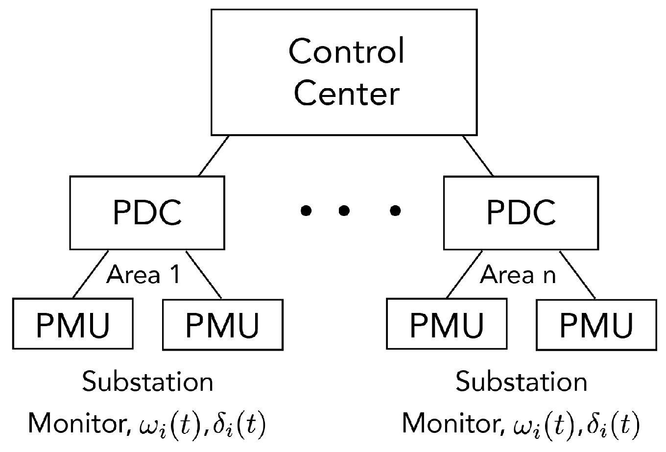
  • We show that the proposed SINDy algorithm can be implemented in a decentralized manner that only requires exchanging the observed phase angle data between the neighbouring nodes of a power grid. Thus, the estimation can be performed locally (e.g., at phasor data concentrator level).
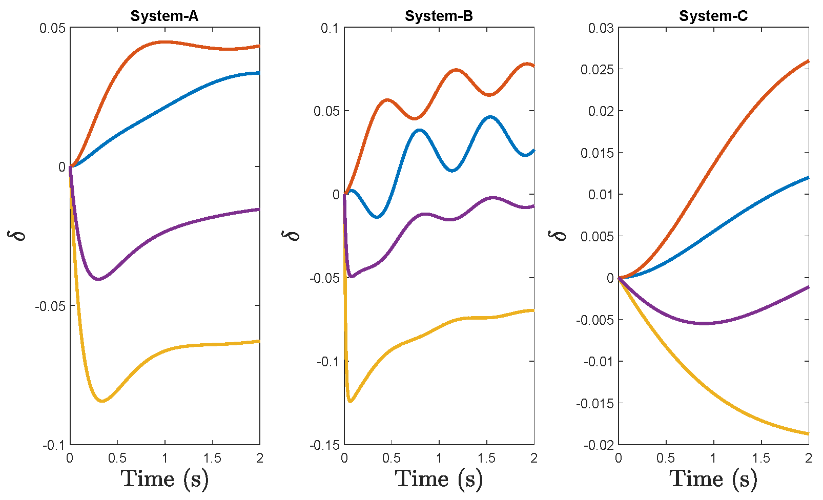
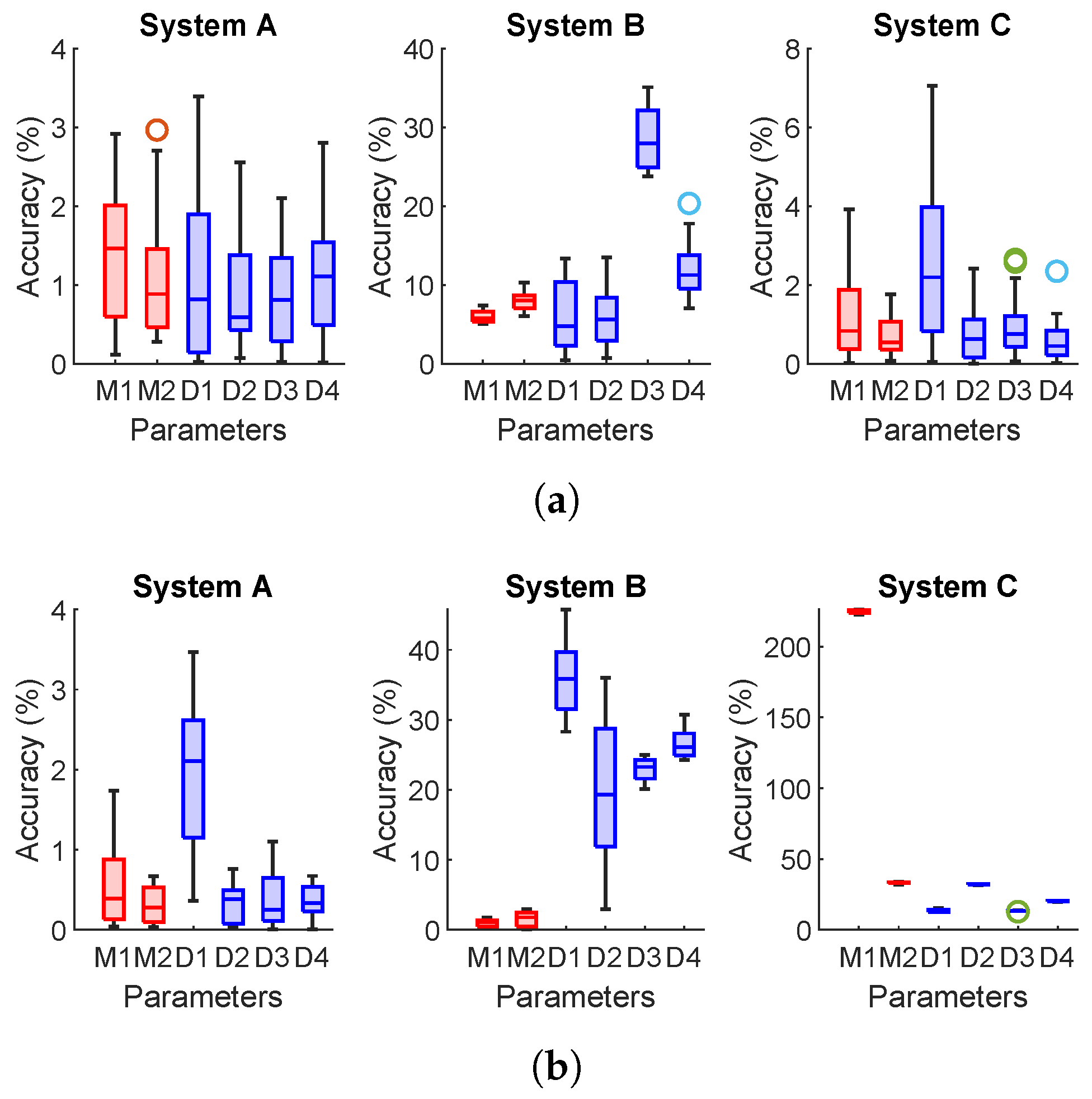
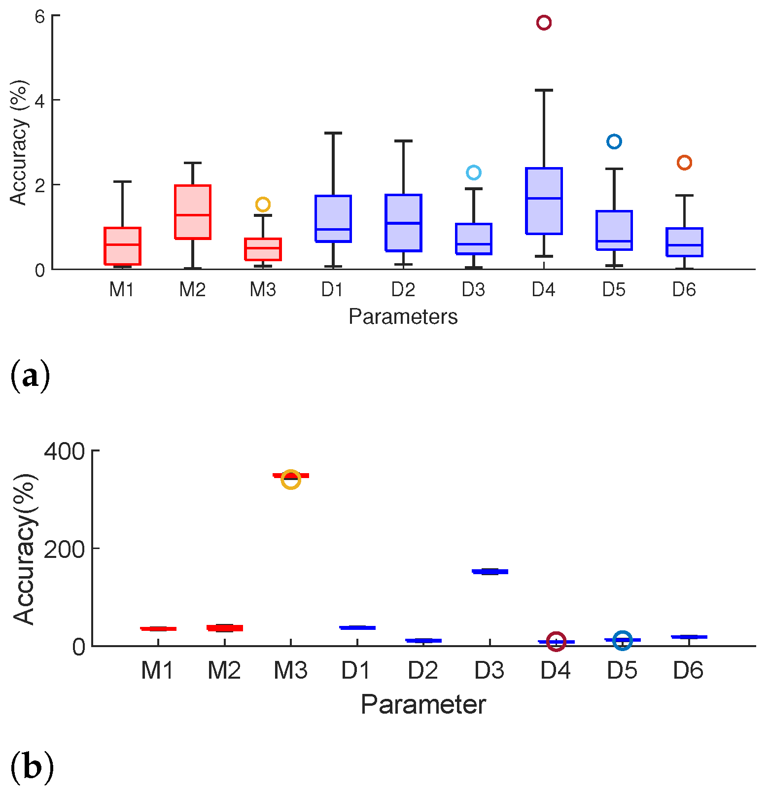
  • We conduct extensive simulations using IEEE bus systems to evaluate and compare the performance of these algorithms.
Our results show that the SINDy algorithm performs well over a wide range of power grid system parameters, i.e., for low and high inertia systems that exhibit fast as well as slow dynamics. This is in contrast to the PINN algorithm that has a large estimation error for systems with slow dynamics. Moreover, since the SINDy algorithm is based on computationally simple linear regression, the computation time is extremely fast. Thus, it is suitable for implementation for real-time parameter estimation in large power systems.
The rest of the paper is organized as follows. Section 2 introduces the system model and the parameter estimation problem. Section 3 describes the SINDy algorithm for power grid parameter estimation and briefly reviews the PINN method. Section 4 considers practical implementation aspects for the SINDy algorithm, such as unknown system model and practical implementation. Section 5 describes the simulation results and Section 6 concludes.

2. Preliminaries

2.1. System Model

We consider a power grid consisting of a set of N = { 1 , , N } buses. The buses are divided into generator buses N G and load buses N L and N = N G N L . The power grid dynamic model is given by [22]:
δ ˙ i = ω i , i N G
M i ω ˙ i = D i ω i P i M j N B i , j sin ( δ i j ) , i N G ,
D i δ ˙ i = P i L j N B i , j sin ( δ i j ) , i N L ,
where δ i is the phase angle deviation at bus i N ,   δ i j = δ i δ j , i , j N and ω i denotes the rotor frequency deviation at the generator buses i N G . The generator inertia coefficient at bus i N G is denoted by M i and the mechanical input power by P i M . The damping coefficients at generator/load buses is denoted by D i i N . B i , j is the susceptance of line i , j . Finally, P i L denotes the load at bus i N L . Note that (1) and (2) model the dynamics of the generator node, whereas (3) models the dynamics at the load nodes.

2.2. Power Grid Parameter Estimation Problem

In this work, we focus on estimating the inertia and damping coefficients, M i , i N G and D i , i N by observing the power grid dynamics. We assume that the system operator has deployed PMUs in the grid, which enables them to monitor the voltage phase angles { δ i ( τ ) } i N , m = 1 , , T and frequency fluctuations { δ ˙ i ( τ ) } i N , τ = 1 , , T , respectively, over a period of time. Herein, we assume a slotted time system with x ( τ ) denoting the value of the signal x at time slot τ , where the slots are sampled at a time interval of T s , and T is the total number of time slots. For instance, according to IEEE/IEC standards, for a 50 Hz system, the PMU sampling frequency can be between 10 to 100 frames per second. Therefore, T s is in the range 10–100 ms [21]. The problem of estimating the inertia and damping coefficients can be posed as an optimisation problem and solve for the unknown parameters. We discuss this in detail in the next sections.

3. Physics-Informed Machine Learning Techniques for Power Grid Parameter Estimation

The focus of this work is on physics-informed machine learning algorithms for the power grid parameter estimation problem. We note that this problem can be treated as a supervised learning problem in which we train a machine learning classifier offline under various system parameter settings. The trained model can be used to perform online inference of the underlying parameters. However, such a black-box approach would require a combinatorially large search across various power grid parameters that must be estimated, and hence, computationally complex. In particular, unlike black-box machine learning algorithms, the physics-informed machine learning leverage the knowledge of the system model to infer parameters from limited observation data.
In this section, we propose a novel data-driven algorithm to solve the parameter estimation problem based on the SINDy algorithm [20], which leverages the knowledge of the differential equations describing the physical system to identify the system parameters. We also briefly describe the PINN approach to estimate the system parameters [16], which also similarly uses the knowledge of the system model.

3.1. Parameter Estimation Using the SINDy Algorithm

The Sparse Identification of Nonlinear Dynamics (SINDy) algorithm applies linear regression to find the system parameters that best represent the observed power grid dynamics [20]. The algorithm exploits the fact that most physical systems have only a few relevant terms that define the dynamics, making the governing equations sparse in a high-dimensional nonlinear function space [20]. In order to formalise this framework for power grid parameter estimation, we define the following additional notations. Let a i ( τ ) and b i ( τ ) be given by
a i ( τ ) = P i M + j N B i , j sin ( δ i j ( τ ) ) , i N G ,
b i ( τ ) = P i L + j N B i , j sin ( δ i j ( τ ) ) , i N L .
Note that the terms a i ( τ ) and b i ( τ ) can be computed by the system operator by monitoring the voltage phase angle dynamics δ i j ( τ ) (using PMU measurements), and the knowledge of the system load fluctuation and generator’s mechanical power. Using (4) and (5), a discretised version of the equations describing the generator and the load bus dynamics in (2) and (3) over τ = 1 , 2 , , T time slots can be written as
ω ˙ i ( 1 ) ω ˙ i ( T ) ω ˙ i = ω i ( 1 ) , a i ( 1 ) ω i ( T ) , a i ( T ) Ω i D i M i 1 M i p i G , i N G ,
δ ˙ i ( 1 ) δ ˙ i ( T ) δ ˙ i = b i ( 1 ) b i ( T ) b i 1 D i p i L , i N L .
Equations (6) and (7) represent the relationship between the generator/load inertia, damping coefficients (that must be estimated), and the observed PMU data. We represent the matrices on the right-hand side of (6) and (7) by Ω i and b i , respectively, and the generator and load parameters by p i G and p i L , respectively. Note that the system operator can compute the elements of Ω i and b i matrices using the frequency and phase angle measurements obtained from the PMUs. Using these measurements, the left-hand side of (6) and (7) can be computed by taking numerical derivatives of δ ˙ i ( τ ) , i N G and δ i ( τ ) , i N L . For noiseless data, the derivative can be computed using the finite difference method. For noisy data, the polynomial interpolation method is better suited [20]. Equations (6) and (7) represent a system of T linear equations. The unknown parameters p i G and p i L can be recovered by solving a linear regression problem. Furthermore, the operator can recover the values of M i and D i from the estimated value of p i G in a straightforward manner. We note that although the framework presented above involves linear regression, it can be applied to power grid system identification problems involving nonlinear system model, such as the one presented in (1)–(3), since the terms inside the nonlinearity can be measured (e.g., the operator can compute sin ( δ i j ( τ ) ) using the measurements δ i j ( τ ) . ) Thus, the SINDy algorithm is applicable for parameter estimation in general nonlinear power system models. The algorithm is depicted in Algorithm 1.
Algorithm 1. SINDy Algorithm.
Input: Phase angle data { δ i ( τ ) } i N , τ = 1 , , T and frequency data { ω i ( τ ) } i N , τ = 1 , , T
Output: p i G and p i L
1:
Monitor phase angle { δ i ( τ ) } i N , τ = 1 , , T and frequency { ω i ( τ ) } i N , τ = 1 , , T data.
2:
From the phase angle data and frequency data, compute { θ ˙ i ( τ ) } i N , τ = 1 , , T .
3:
Construct the vector and the vector θ ˙ and the matrix Ω from the phase angle and frequency measurements.
4:
Using θ ˙ and Ω , solve for p i G and p i L using the LASSO algorithm.
5:
Output p i G and p i L

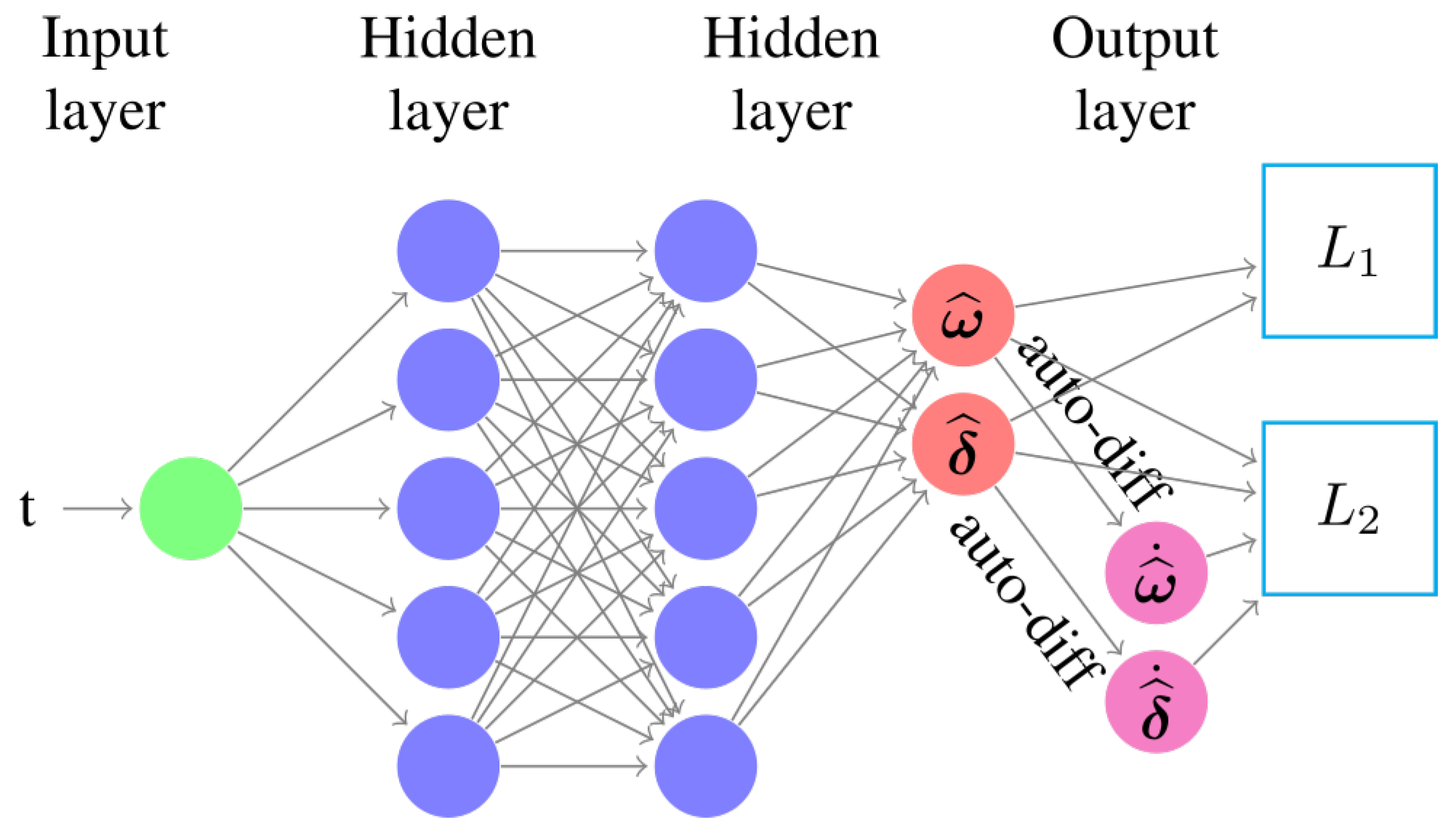
3.2. Parameter Estimation Based on Physics-Informed Neural Networks

We also briefly describe the PINN framework [23,24] applied to power system parameter estimation as proposed in [16]. The overall PINN framework is shown in Figure 1. It uses NNs to approximate the solution ω i ( t ) and δ i ( t ) that solves (1)–(3). Let ω ^ i ( t , ϕ ) and δ ^ i ( t , ϕ ) denote the respective NN approximations as shown in Figure 1. Herein, ϕ represents the weights of the NN, which are trained to minimize the following losses.

3.2.1. Mean Squared Loss

The first loss term involves minimizing the mean square loss between the observed measurements ω i ( t ) and δ i ( t ) and their NN approximations, i.e.,
L 1 ( ϕ ) = 1 T τ = 1 T ( i N G ( ω ^ i ( τ , ϕ ) ω i ( τ ) ) 2 + i N ( δ ^ i ( τ , ϕ ) δ i ( τ ) ) 2 ) .

3.2.2. Physics-Based Loss

The system dynamics are incorporated as a second loss function. Specifically, let us define
f i ( 1 ) = δ ^ ˙ i ω ^ i , i N G
f i ( 2 ) = M i ω ^ ˙ i + D i ω ^ i P i M   + j N B i , j sin ( δ ^ i j ) , i N G ,
f i ( 3 ) = D i δ ^ ˙ i + P i L + j N B i , j sin ( δ ^ i j ) , i N L ,
where in the above, we have dropped the notations showing the dependency of f i ( 1 ) and f i ( 2 ) on ( τ , ϕ ) and f i ( 3 ) on ( τ , ϕ , p ) , where p = [ p G ; p L ] , and simplicity. Note that in the above, the derivatives are computed using NN’s automatic differentiation. The physics-based loss function is then given by
L 2 ( ϕ , p ) = 1 T τ = 1 T ( i N G ( f i ( 1 ) ( τ , ϕ ) ) 2 + i N G ( f i ( 2 ) ( τ , ϕ ) 2 + i N L ( f i ( 3 ) ( τ , ϕ , p ) 2 ) .
Note that the above loss function depends both on the NN weights ϕ and the system parameters p . The NN is trained using the observed measurements { δ i ( τ ) } i N , τ = 1 , , T and { ω i ( τ ) } i N , τ = 1 , , T as follows:
ϕ * , p * = arg min ϕ , p L 1 ( ϕ ) + L 2 ( ϕ , p )
Note that when the sum of these two losses is minimized, we ensure two criteria: (1) the output of the NN replicates the observed system dynamics, (2) f i ( 1 ) , f i ( 2 ) , and f i ( 3 ) are close to zero, which in turn implies that (1)–(3) are satisfied. This implies that the estimated parameters best fit the observed data.

4. Practical Implementation Aspects

In this section, we cover some practical implementation aspects for the proposed SINDy algorithm in the power system identification problem. In particular, we examine how the system operator can perform system identification, i.e., identifying the model and the underlying parameters when they do not have an accurate knowledge of the differential equations describing the system, and a decentralized implementation of the algorithms.

4.1. Unknown System Model

The algorithm described in the previous section assumes that the system operator has the precise knowledge of the differential equations governing the power grid dynamics (i.e., Equations (1)–(3)). However, this knowledge may not be available precisely for many real-world systems.
In such cases, the system operator can create a dictionary of candidate linear and nonlinear terms based on the observed data to construct the right-hand side matrices of (6) and (7), respectively (i.e., Ω i and b i ) [20]. An example of the dictionary functions to estimate the generator parameters, Θ i ( δ , ω ) , is presented in (15). (Note that in (15), we use { δ i ( τ ) } i = 1 N as a short-hand notation for a smaller matrix whose columns are given by δ i ( τ ) , i = 1 , , N . ) The columns of the matrix Θ i ( δ , ω ) represent candidate linear and nonlinear functions that can potentially model the generator dynamics observed in (2). The choice of these functions can be arbitrary. Moreover, since we assume that the operator is unaware of the precise system model, they can choose a large number of such candidate functions of the observed measurements.
The system identification and parameter estimation problem now becomes one of identifying which of the chosen dictionary functions are actually contributing to the observed system dynamics. In practice, only a few of the terms may be the real contributors to the observed dynamics. Thus, the generator parameters p i G can be estimated as the sparsest solution that satisfies the following equation
ω ˙ i = Θ i ( δ , ω ) p i G .
In this case, the sparse solution determines which of the candidate terms are contributing to the observed dynamics. Moreover, the sparse solution also avoids an NP-hard combinatorial brute-force search across all possible term combinations.
Θ i ( δ , ω ) = | | | | | | { δ i ( τ ) } i = 1 N { ω i ( τ ) } i = 1 N { ( δ i ( τ ) ) 2 } i = 1 N { ( ω i ( τ ) ) 2 } i = 1 N { sin ( δ i j ( τ ) ) } i , j = 1 N | | | | | | ,
Note that (14) is a system of T linear equations with M unknown variables, where M is the size of the dictionary functions. In general, T M , since PMUs have a high sampling frequency (e.g., 50 measurement samples per second [21]). To promote sparsity in the estimated value of p i G , we use the LASSO algorithm, which applies an L1-regularisation term to promote sparsity. The optimisation problem corresponding the LASSO algorithm is given by [25]
p ^ i G = arg min p i G | | Θ i ( δ , ω ) p i G ω ˙ i | | 2 + λ | | p i G | | 1 , i = 1 , | G | .
Herein, | | p i G | | 1 represents a penalty term that and λ > 0 is a scaling parameter. The weight λ plays an important role in parameter estimation. Specifically, if λ is set to a low value, then this will result in a solution that is not sparse leading to incorrect parameter estimates. This is because there may be multiple combination of the parameters/dictionary functions that may lead to similar dynamics (i.e., the solution to (16) may not be unique when λ is set to zero or a low value). On the other hand, if λ is set to a high value, then this will favour an overly sparse solution in which most of the parameters are estimated to be zero. Thus, the value of λ must be carefully calibrated to obtain accurate estimates of the parameters. The system operator can tune this parameter by offline simulations, based on historical measurements and the knowledge of the true values of the parameters under consideration. For instance, in our simulations for the IEEE 6-bus system, we found that setting λ = 0.1 leads to accurate parameter estimates.
We note that the knowledge of the physics of the system under consideration (albeit an approximate or an inaccurate one) can significantly narrow down the choice of the candidate functions. This is because the system operator can make a reasonable guess on what type of candidate functions might be relevant in practice. For instance, it is well known that sine of the difference between the nodal phase angles is an important quantity in power grids that determines the power flow in transmission lines. Similarly, the governor’s droop control implies that a linear or quadratic function of the frequency will be a relevant candidate function for such systems. Thus, even an approximate knowledge of the underlying system model can significantly reduce the complexity associated with the parameter estimation process. We also note that recent work has proposed analytical methods to construct the observable functions for parameter estimation in this scenario [26]. We defer a detailed analysis in this regard to future work.

4.2. Decentralised Implementation

The SINDy algorithm applied to power system identification can be integrated into existing wide-area monitoring systems (WAMS). The WAMS network, shown in Figure 2, has a hierarchical structure in which the PMUs installed at the substation monitor the phase angle/frequency measurements. The monitored signals and transmitted to a phasor data concentrator (PDC), and subsequently to a control center (CC) using the underlying communication network (usually optic fiber communication). The proposed SINDy algorithm can be implemented in a decentralized manner within the WAMS architecture with limited information exchange between the nodes. We elaborate on this in the following.
Recall that the algorithm involves solving for the unknown terms in (6) and (7). This in turn requires the following signals at each node i N : (i) ω i , (ii) δ i , (iii) { δ j } j N i , where N i are the neighbouring nodes of node i . Note that (i) and (ii) can be monitored locally at individual nodes, and (iii) only requires information exchange with only the neighboring nodes. Thus, the SINDy algorithm can be implemented locally with limited information exchange between the nodes.

4.3. Knowledge of System Parameters

Note that in the implementation of SINDy algorithm requires the knowledge of power grid transmission line parameters (line impedances B i j ), load perturbation, and generator’s mechanical power. Line impedances B i j are quantities that do not change frequently, so they can be estimated using steady-state measurements based on a reasonably large observation window [4,5,6,7]. The load fluctuations can be estimated by including them as additional variables in the SINDy algorithm. The mechanical power of the generator can be measured directly. For instance, if the generator adopts a proportional–integral–derivative (PID) control such as P i M = K p ω i + K I δ i , where K p and K I are the generator’s proportional/integral coefficients, then P i M can be calculated by using the frequency/phase angle measurements (assuming that the generator’s constants such as the proportional/integral constants are known to the system operator, otherwise they must be estimated as well).

5. Simulation Results

In this section, we present simulation results to show the effectiveness of the SINDy algorithm and compare its performance against PINN and UKF algorithms.
For our simulations, we obtain the power grid topological data from the MATPOWER simulator. To generate the dataset corresponding to power grid dynamics, we simulate the differential equations in (1)–(3) using the ode-45 function of MATLAB. We use the polynomial interpolation method to take numerical derivatives and solve the linear regression problems using MATLAB. For the PINN algorithm, we use the code provided in [27] that is implemented using Tensorflow. We use a multilayer perceptron for PINN with two hidden layers each with 30 neurons and the automatic differentiation to calculate the gradients. The NN is trained using the ADAM optimizer.
We first compare the performance of the algorithms using the 4-bus 2-generator model. We use three simulation settings as in [16]–system A that is considered as the standard system, system B with faster dynamics (as compared to system A), and system C with slower dynamics. The parameter values are listed in the Appendix A. The phase angle dynamics corresponding to the three settings obtained by adding a load perturbation of 0.1 pu. at Bus 3 are shown in Figure 3. To generate the noisy signal, we add Gaussian noise whose standard deviation σ is set to 5 % of the measurement’s value. Note that this ensures a signal-to-noise ratio (SNR) of approximately 20–30 dB ( S N R = 20 l o g 10 ( 1 / 0.05 ) ), which is reasonable for PMUs [28]. We consider 100 samples per second (thus, a PMU sampling interval of 0.01 s) and a time horizon of 2 s. Thus, T = 2 × 100 = 200 .
The error in parameter estimation (boxplots) considering the 4-bus 2-generator model is shown in Figure 4 for the SINDy and PINN algorithms, respectively, over 20 simulation runs. As evident from the figure, both the PINN and the SINDy algorithms have a high estimation accuracy for System A, and most of the unknown parameters are estimated within 3–4 percent of the original value. Both the algorithms also have similar performance for System B, i.e., the system fast dynamics. We observe that M parameters are recovered with good accuracy, but the D parameters have higher error (within 40 % ). However, in terms of the actual value, the true and estimated parameters are close, e.g., D 4 = 0.02 and D ^ 4 = 0.028 .
The most notable difference between the two algorithms can be seen for System C which has slow dynamics. While the PINN algorithm has a high estimation error for some parameters (up to 200 % ), the SINDy algorithm has a low estimation error for this case as well. As noted in [16], the large error for the PINN algorithm can be attributed to the challenges in training the NN. Specifically, for the system with slow dynamics, the optimization landscape is flat, and hence, no direction of the gradient dominates. In contrast, the SINDy algorithm, which is based on a computationally simple linear regression faces no such obstacles.
For a comparison with the UKF approach, we refer to the results in [16], where it is noted that the UKF algorithm does not perform well for System B (with fast dynamics). This is because the UKF algorithm cannot capture fast information dynamics that occur within a few time steps. Thus, we conclude that the SINDy algorithm has a better performance compared to the UKF and the PINN approach over a wide range of system parameters.
Another significant advantage of the SINDy algorithm is its fast computing time. The simulations for the SINDy algorithm are conducted using a Macbook Pro 2.3 GHz Dual-Core Intel Core i5 processor with 8 GB RAM and we enlist the run time in Table 1. It can be noted that the SINDy algorithm is computationally extremely fast compared to the PINN algorithm (by about 1000 times for the 4-bus system) since it does not involve training a neural network. Furthermore, from the table, we note that the computing time is also extremely low for larger bus systems (results to be enlisted next). Thus, this approach is better suited for real-time parameter estimation.

5.1. Dependence on the Observation Time Window

Next, we examine the dependency of the estimation error on the observation time window for the SINDy algorithm. Once again, we consider the 4-bus 2-generator system. In Table 2, we enlist the mean accuracy of D 1 over 20 trials (we observed that the estimation error for this parameter is the greatest among all the parameters). We also consider two different noise levels, i.e., σ = [ 5 % , 10 % ] of the measurement’s value. It can be noted that the algorithm can achieve low estimation error with data from about 2 s observation time window. Furthermore, more noisy data requires a slightly larger observation time window, and the estimation error is slightly higher, which is expected.

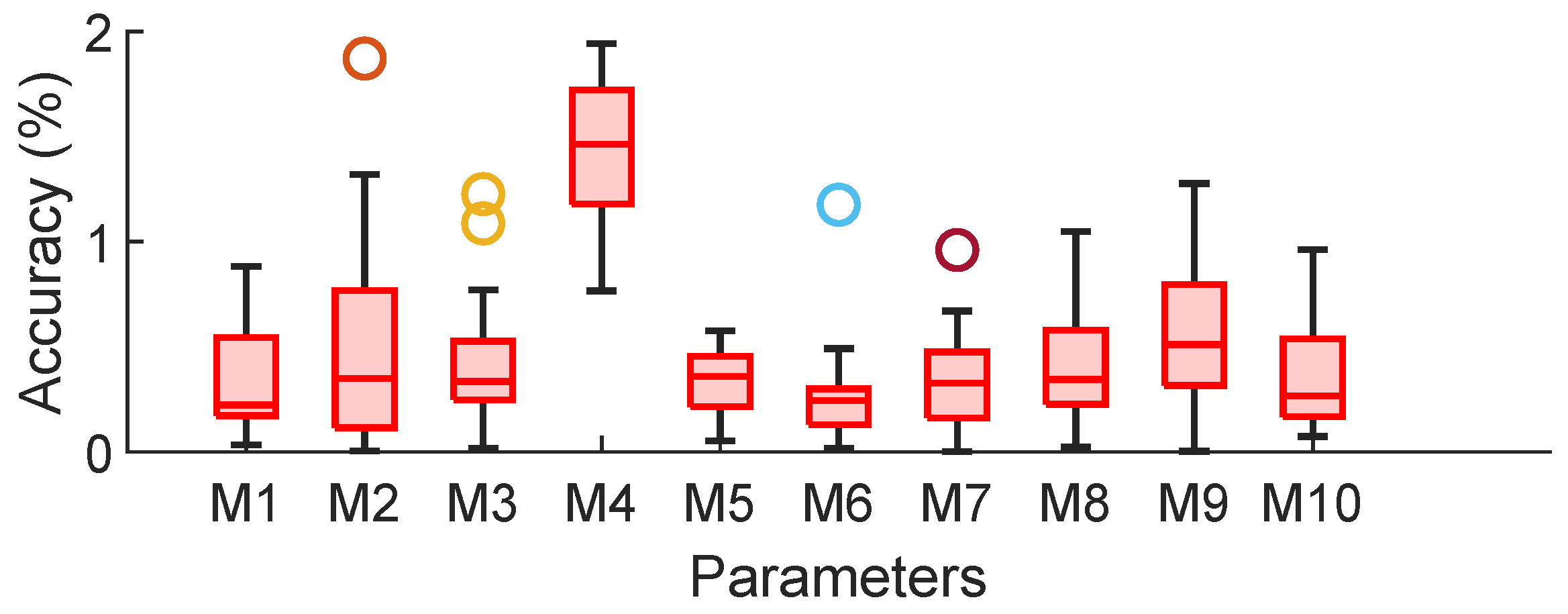
5.2. Simulations with Larger Bus Systems

We also plot the error in parameter estimation for the IEEE-6 bus and 39 bus systems. For brevity, we only plot the accuracy of the inertia estimations ( M i ) for the IEEE-39 bus system (note the 39-bus system has 10 generators and 29 loads). The simulation parameters are once again listed in Appendix A and the results are plotted in Figure 5 and Figure 6. The dynamics are generated by applying a load perturbation of 0.1 pu at bus 4 and bus 1 for the IEEE 6-bus and 39-bus systems, respectively. It can be observed that the SINDy approach achieves high accuracy even for larger bus systems. On the other hand, we did not observe good estimation results for the PINN algorithm (as shown in Figure 5b) using the code provided in [27]. We believe further data processing may be required to ensure the scalability of the PINN algorithm to large systems.

5.3. Simulations with Unknown System Model

We further perform simulations when the operator does not have the exact knowledge of the underlying system model. Specifically, while applying the SINDy algorithm for parameter estimation, we do use the Ω i matrix in the right-hand side of (6) in the estimation process. Rather, we create a dictionary of candidate functions Θ i ( δ , ω ) as described in Section 4.1. We consider a number of linear and nonlinear functions of the frequency and phase angle measurements within the dictionary. An example of the estimation of the inertia and damping coefficients of the generator at node 1 of the 6-bus system is illustrated in the following. The actual differential equations governing the evolution of the frequency at generator bus 1 is given by
ω ˙ 1 = ω 1 + 0.16 4 sin ( δ 12 ) 4 sin ( δ 14 ) 2.66 sin ( δ 15 )
The predicted coefficients of the differential equation produced by the SINDy algorithm as applied in Section 4.1 (we set λ = 0.1 in (16)) is given by
ω ˙ 1 = 0.98 ω 1 + 0.012 ω 2 + 0.003 ω 3 + 0.12 ω 1 2 + 0.001 ω 2 2 + 0.001 ω 3 2 + 0.155 4.12 sin ( δ 12 ) 0 sin ( δ 13 ) 4.18 sin ( δ 14 ) 4.12 sin ( δ 15 ) 0.012 sin ( δ 16 )
Note that the two equations match closely, confirming the effectiveness of the SINDy algorithm in parameter estimation even when the system operator does not have an accurate knowledge of the physical model of the system under consideration.

5.4. Simulations with Non-Gaussian Noise

We also conducted simulations considering non-Gaussian noise, since some recent work based on real-world experiments shows that PMU noise data can be better modeled with Student’s t or logistic distributions [29]. We added logistic noise whose parameters are adjusted to obtain a standard deviation of 0.01 pu. We observed that the performance of the SINDy algorithm under non-Gaussian noise conditions is similar to the Gaussian case. For brevity, exclude the results here, since they are similar to Figure 4.

6. Conclusions and Future Work

Parameter estimation is an important and necessary tool in safe power grid operation. Realtime estimation of unknown system parameter can ensure the grid is stable. In this work, we propose a physics-informed machine learning algorithm to estimate power grid parameters from the observed phase angle/frequency data. The proposed method, based on the SINDy algorithm, applies linear regression to estimate the power grid parameters that best describe the observed data. The novelty of the proposed algorithm lies in the simplicity of the method. The main contribution of this paper is that the algorithm is applicable for general nonlinear power grid models including the standard, fast, and slow dynamics system. The simulation results show the accuracy of the algorithm is within 40 % for all systems. Compared to PINN algorithm not only it is significantly better for slow dynamics but also the execution is faster. We extend this algorithm to cases when the operator does not have an accurate knowledge of the underlying physical model of the system. Furthermore, we present a decentralised implementation of the proposed SINDy algorithm, where the grid parameters can be estimated by limited information exchange between the neighbouring nodes of the power grid. Simulation results conducted on the benchmark power grid bus systems show that the proposed algorithm performs well under various parameter settings, and bus systems. Our future work includes: (i) an analysis of the optimal placement of PMUs to ensure reliable parameter estimation. To this end, combining results from compressed sensing and SINDy to infer parameters from subsampled data will be useful [20,30]. (ii) Application to higher-order generator models and (iii) verifying the parameter estimation using hardware-in-the-loop simulation.

Author Contributions

Conceptualization, S.L. and C.M.; methodology, S.L. and S.S.; software, S.L. and S.S.; validation, S.L. and S.S.; writing, S.L., S.S. and C.M. All authors have read and agreed to the published version of the manuscript.

Funding

This work has been supported by the PETRAS National Centre of Excellence for IoT Systems Cybersecurity, which has been funded by the UK EPSRC under grant number EP/S035362/1.

Conflicts of Interest

The authors declare no conflict of interest.

Appendix A. Simulation Parameters

All the values are provided in pu.

Appendix A.1. 4-Bus System

P 1 M = 0.1 ,   P 2 M = 0.2 ,   P 1 L = 0.1 ,   P 2 L = 0.2
System A:
M 1 = 0.3 ,   M 2 = 0.2
D 1 D 4 : 0.15 ,   0.3 ,   0.25 ,   0.25
System B:
M 1 = 0.02 ,   M 2 = 0.03
D 1 D 4 : 0.015 ,   0.015 ,   0.02 ,   0.04
System C:
M 1 = 5.2 ,   M 2 = 4.0
D 1 D 4 : 3.8 ,   4.3 ,   10.5 ,   8.3

Appendix A.2. IEEE 6-Bus System

M 1 M 3 : 1.25 ,   0.34 ,   0.16
D 1 D 6 : 1.25 ,   0.68 ,   0.32 ,   1 ,   1 ,   1
P 1 M = 0.2 ,   P 2 M = 0.1 ,   P 1 L = 0.1 ,   P 2 L = 0.2

Appendix A.3. IEEE 39-Bus System

M 1 = 2.3186 ,   M 2 : M 8 = 2.6419 ,   M 9 : M 10 = 2.4862 .
D i = 2 , i N G
D i = 0.1 ,   i N L
P 33 M = 0.2 ,   P 19 L = 0.2 .

References

  1. Kosterev, D.; Taylor, C.; Mittelstadt, W. Model validation for the August 10, 1996 WSCC system outage. IEEE Trans. Power Syst. 1999, 14, 967–979. [Google Scholar] [CrossRef] [Green Version]
  2. Schweppe, F.C.; Wildes, J. Power System Static-State Estimation, Part I: Exact Model. IEEE Trans. Power Appar. Syst. 1970, PAS-89, 120–125. [Google Scholar] [CrossRef] [Green Version]
  3. Schweppe, F.C.; Rom, D.B. Power System Static-State Estimation, Part II: Approximate Model. IEEE Trans. Power Appar. Syst. 1970, PAS-89, 125–130. [Google Scholar] [CrossRef]
  4. Li, X.; Poor, H.V.; Scaglione, A. Blind topology identification for power systems. In Proceedings of the IEEE International Conference on SmartGrid Communications (SmartGridComm), Vancouver, BC, Canada, 21–24 October 2013; pp. 91–96. [Google Scholar]
  5. Grotas, S.; Yakoby, Y.; Gera, I.; Routtenberg, T. Power Systems Topology and State Estimation by Graph Blind Source Separation. IEEE Trans. Signal Process. 2019, 67, 2036–2051. [Google Scholar] [CrossRef] [Green Version]
  6. Weng, Y.; Liao, Y.; Rajagopal, R. Distributed Energy Resources Topology Identification via Graphical Modeling. IEEE Trans. Power Syst. 2017, 32, 2682–2694. [Google Scholar] [CrossRef]
  7. Deka, D.; Backhaus, S.; Chertkov, M. Structure Learning in Power Distribution Networks. IEEE Trans. Control Netw. Syst. 2018, 5, 1061–1074. [Google Scholar] [CrossRef]
  8. Tate, J.E.; Overbye, T.J. Line Outage Detection Using Phasor Angle Measurements. IEEE Trans. Power Syst. 2008, 23, 1644–1652. [Google Scholar] [CrossRef]
  9. Zhao, Y.; Chen, J.; Poor, H.V. A Learning-to-Infer Method for Real-Time Power Grid Multi-Line Outage Identification. IEEE Trans. Smart Grid 2020, 11, 555–564. [Google Scholar] [CrossRef] [Green Version]
  10. Yu, Z.; Chin, W. Blind False Data Injection Attack Using PCA Approximation Method in Smart Grid. IEEE Trans. Smart Grid 2015, 6, 1219–1226. [Google Scholar] [CrossRef]
  11. Lakshminarayana, S.; Kammoun, A.; Debbah, M.; Poor, H.V. Data-Driven False Data Injection Attacks Against Power Grids: A Random Matrix Approach. IEEE Trans. Smart Grid 2021, 12, 635–646. [Google Scholar] [CrossRef]
  12. Ariff, M.A.M.; Pal, B.C.; Singh, A.K. Estimating Dynamic Model Parameters for Adaptive Protection and Control in Power System. IEEE Trans. Power Syst. 2015, 30, 829–839. [Google Scholar] [CrossRef] [Green Version]
  13. Valverde, G.; Kyriakides, E.; Heydt, G.T.; Terzija, V. Nonlinear Estimation of Synchronous Machine Parameters Using Operating Data. IEEE Trans. Energy Convers. 2011, 26, 831–839. [Google Scholar] [CrossRef]
  14. Rouhani, A.; Abur, A. Constrained Iterated Unscented Kalman Filter for Dynamic State and Parameter Estimation. IEEE Trans. Power Syst. 2018, 33, 2404–2414. [Google Scholar] [CrossRef]
  15. Huang, R.; Diao, R.; Li, Y.; Sanchez-Gasca, J.; Huang, Z.; Thomas, B.; Etingov, P.; Kincic, S.; Wang, S.; Fan, R.; et al. Calibrating Parameters of Power System Stability Models Using Advanced Ensemble Kalman Filter. IEEE Trans. Power Syst. 2018, 33, 2895–2905. [Google Scholar] [CrossRef]
  16. Stiasny, J.; Misyris, G.S.; Chatzivasileiadis, S. Physics-Informed Neural Networks for Non-Linear System Identification Applied to Power System Dynamics. 2020. Available online: https://arxiv.org/abs/2004.04026 (accessed on 28 December 2021).
  17. Zhao, J.; Gómez-Expósito, A.; Netto, M.; Mili, L.; Abur, A.; Terzija, V.; Kamwa, I.; Pal, B.; Singh, A.K.; Qi, J.; et al. Power System Dynamic State Estimation: Motivations, Definitions, Methodologies, and Future Work. IEEE Trans. Power Syst. 2019, 34, 3188–3198. [Google Scholar] [CrossRef]
  18. Qi, J.; Sun, K.; Kang, W. Optimal PMU Placement for Power System Dynamic State Estimation by Using Empirical Observability Gramian. IEEE Trans. Power Syst. 2015, 30, 2041–2054. [Google Scholar] [CrossRef] [Green Version]
  19. Rouhani, A.; Abur, A. Observability Analysis for Dynamic State Estimation of Synchronous Machines. IEEE Trans. Power Syst. 2017, 32, 3168–3175. [Google Scholar] [CrossRef]
  20. Brunton, S.L.; Proctor, J.L.; Kutz, J.N. Discovering governing equations from data by sparse identification of nonlinear dynamical systems. Proc. Natl. Acad. Sci. USA 2016, 113, 3932–3937. [Google Scholar] [CrossRef] [Green Version]
  21. IEEE/IEC International Standard—Measuring Relays and Protection Equipment—Part 118-1: Synchrophasor for Power Systems—Measurements; IEC/IEEE 60255-118-1:2018; IEEE: Manhattan, NY, USA, 2018; pp. 1–78.
  22. Kundur, P.; Balu, N.; Lauby, M. Power System Stability and Control; McGraw-Hill Education: New York, NY, USA, 1994. [Google Scholar]
  23. Raissi, M.; Perdikaris, P.; Karniadakis, G. Physics-Informed Neural Networks: A Deep Learning Framework for Solving Forward and Inverse Problems Involving Nonlinear Partial Differential Equations. J. Comput. Phys. 2019, 378, 686–707. [Google Scholar] [CrossRef]
  24. Lagaris, I.E.; Likas, A.; Fotiadis, D.I. Artificial neural networks for solving ordinary and partial differential equations. IEEE Trans. Neural Netw. 1998, 9, 987–1000. [Google Scholar] [CrossRef] [Green Version]
  25. Tibshirani, R. Regression Shrinkage and Selection via the Lasso. J. R. Stat. Soc. Ser. B 1996, 58, 267–288. [Google Scholar] [CrossRef]
  26. Netto, M.; Susuki, Y.; Krishnan, V.; Zhang, Y. On Analytical Construction of Observable Functions in Extended Dynamic Mode Decomposition for Nonlinear Estimation and Prediction. IEEE Control Syst. Lett. 2021, 5, 1868–1873. [Google Scholar] [CrossRef]
  27. Stiasny, J.; Misyris, G.S.; Chatzivasileiadis, S. 2020. Available online: https://github.com/jbesty/PINN_system_identification (accessed on 28 December 2021).
  28. Brown, M.; Biswal, M.; Brahma, S.; Ranade, S.J.; Cao, H. Characterizing and quantifying noise in PMU data. In Proceedings of the IEEE Power and Energy Society General Meeting (PESGM), Boston, MA, USA, 17–21 July 2016; pp. 1–5. [Google Scholar] [CrossRef]
  29. Wang, S.; Zhao, J.; Huang, Z.; Diao, R. Assessing Gaussian Assumption of PMU Measurement Error Using Field Data. IEEE Trans. Power Deliv. 2018, 33, 3233–3236. [Google Scholar] [CrossRef]
  30. Brunton, S.L.; Proctor, J.L.; Tu, J.H.; Kutz, J.N. Compressed sensing and dynamic mode decomposition. J. Comput. Dyn. 2015, 2, 165–191. [Google Scholar] [CrossRef]
Figure 1. PINN network showing input output and the losses. The unknown parameters are declared as Tensorflow variables and estimated by the optimiser.
Sustainability 14 02051 g001
Figure 2. Schematic diagram for the implementation of the proposed SINDy algorithm in wide-area monitoring systems.
Sustainability 14 02051 g002
Figure 3. Frequency dynamics for the 4-bus system. Left figure is for the standard system (System A), middle is for the faster dynamics (System B), and the right figure is for slower dynamics (System C). For System C, the gradient of the waveform is not enough for PINN to learn the parameters accurately.
Sustainability 14 02051 g003
Figure 4. Box plot showing error in parameter estimation for 4-bus 2-generator model. Red and blue boxes represent the error in unknown parameters M and D, respectively. The circles represent the outlier data. (a) SINDy algorithm. (b) PINN algorithm.
Sustainability 14 02051 g004
Figure 5. Error in parameter estimation for IEEE-6 bus system. Red and blue boxes represent the error in unknown parameters M and D, respectively. (a) SINDy algorithm. Average error for both M and D is below 2%. (b) PINN algorithm. Average errors M and D are close to 400% and 200%, respectively.
Sustainability 14 02051 g005
Figure 6. Error in parameter estimation for IEEE-39 bus system.
Sustainability 14 02051 g006
Table 1. Computation times for the SINDy and PINN algorithms.
Algorithm (Number of Buses)Execution Time (s)
PINN (4 bus)90 s (from [16])
SINDy (4 bus) 8.4 ms
SINDy (IEEE 6-bus) 10.5 ms
SINDy (IEEE 39-bus) 86 ms
Table 2. Mean estimation error of D 1 as a function of the observation time window and noise level for the SINDy algorithm over 20 runs. The results correspond to the 4-bus 2-generator system, System A.
Time Window (s) σ = 5 % σ = 10 %
0.5 s 22.2 % 40.3 %
1 s 12.2 % 21.84 %
2 s 1.12 % 2.82 %
5 s 1 % 2.46 %
Publisher’s Note: MDPI stays neutral with regard to jurisdictional claims in published maps and institutional affiliations.

