

Techno-Economic Analysis of Non-Wire Alternative (NWA) Portfolios Integrating Energy Storage Systems (ESS) with Photovoltaics (PV) or Demand Response (DR) Resources Across Various Load Profiles

Abstract
1. Introduction
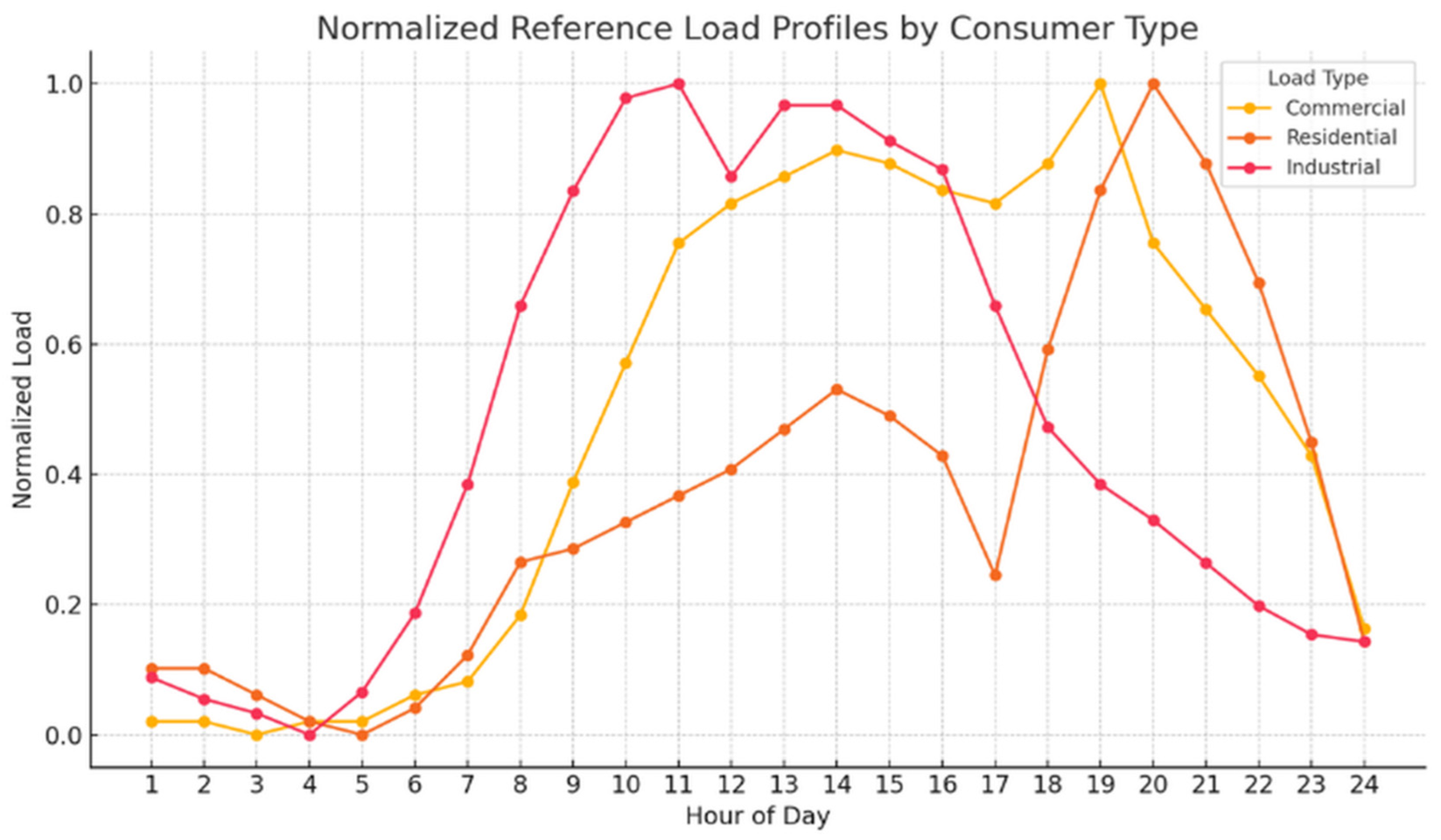
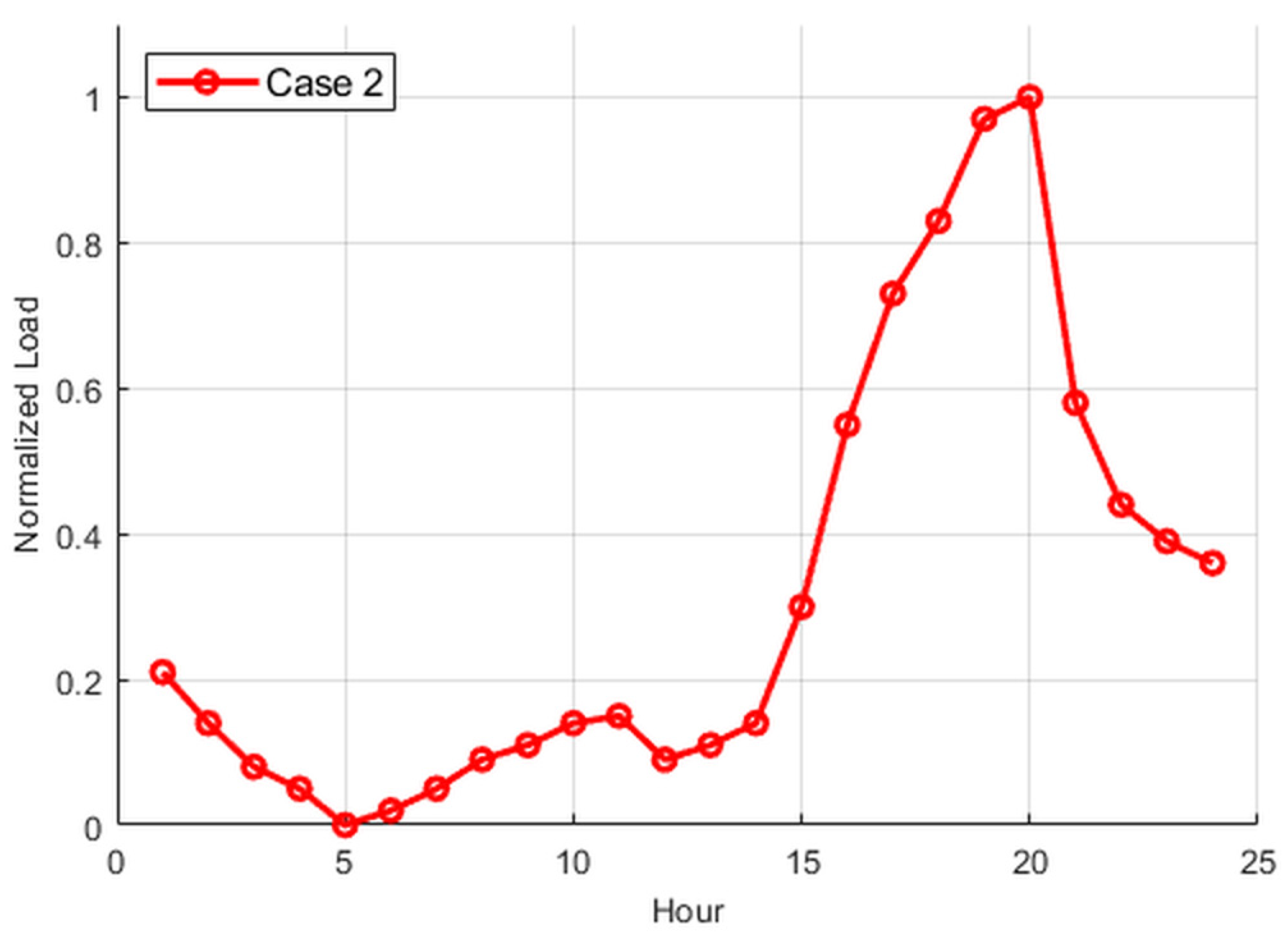
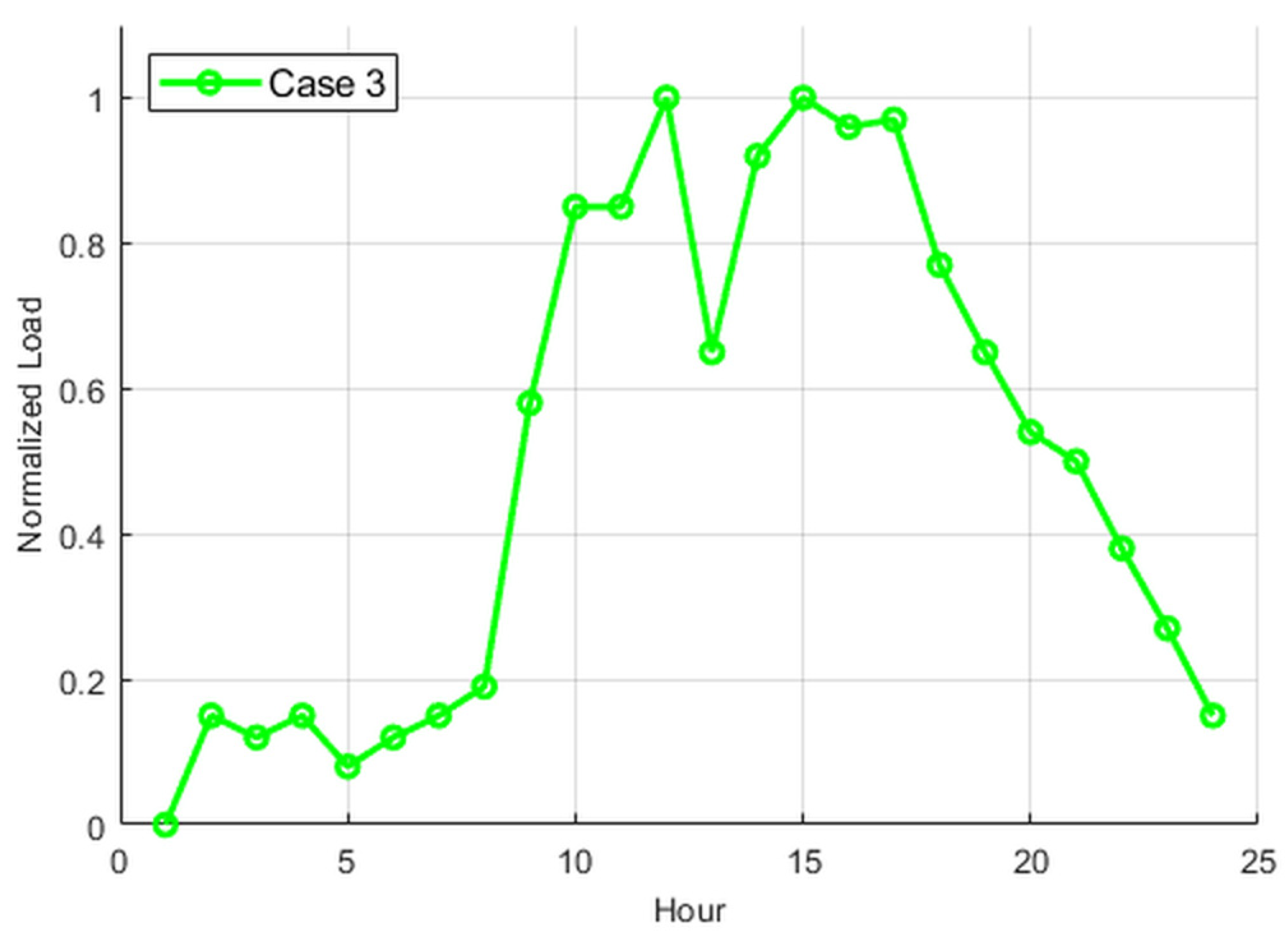
2. Load Profile Characteristics
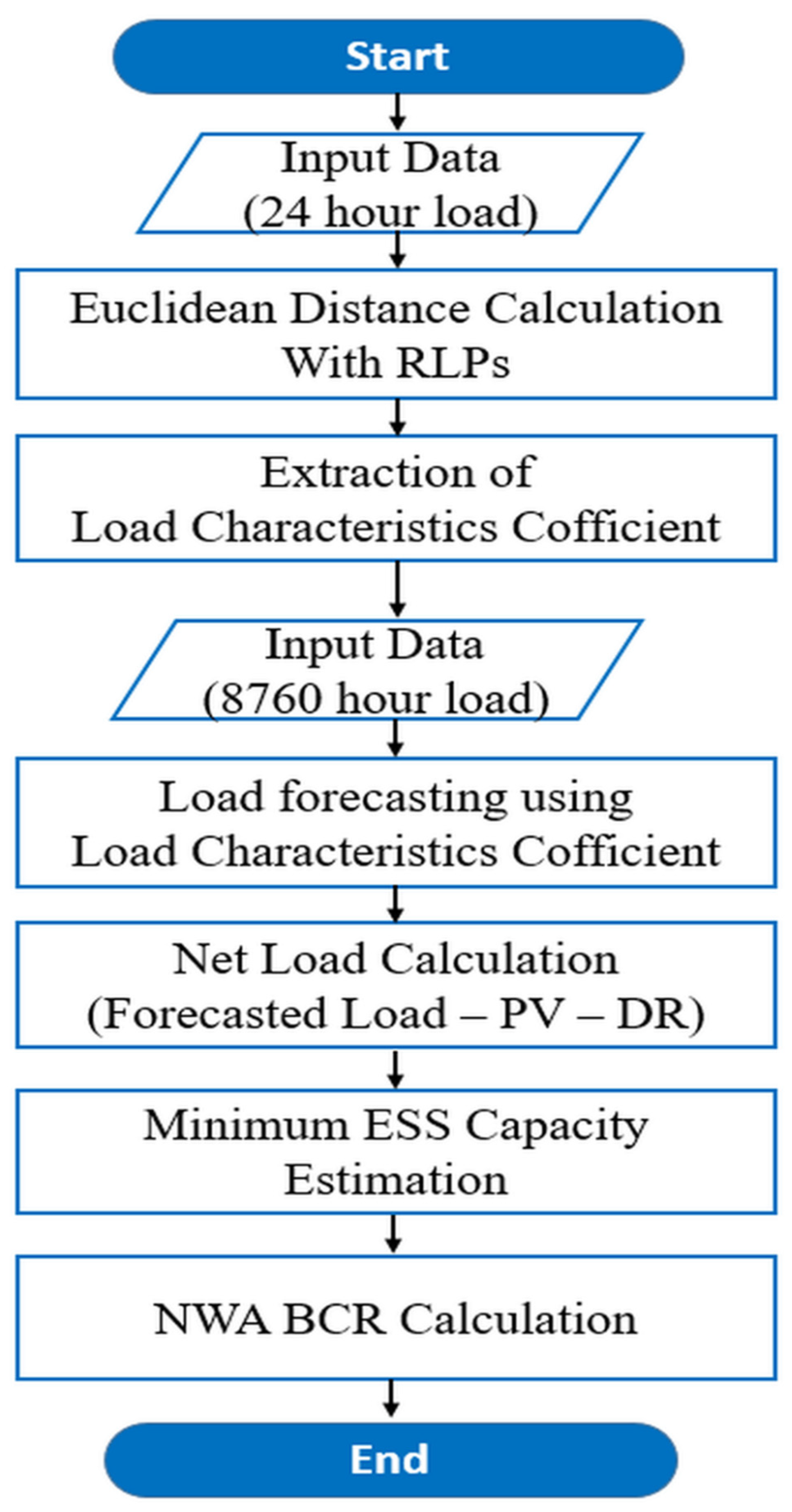
3. NWA-BCA Prediction Model
3.1. Load Characteristic Coefficient
3.2. Load Forecasting Method
3.3. ESS Capacity Estimation
3.3.1. Objective Function
3.3.2. Charge and Discharge Power Limit Constraints
3.3.3. Prohibition of Simultaneous Charging and Discharging Constraints
3.3.4. SOC Dynamics and Limit Constraints
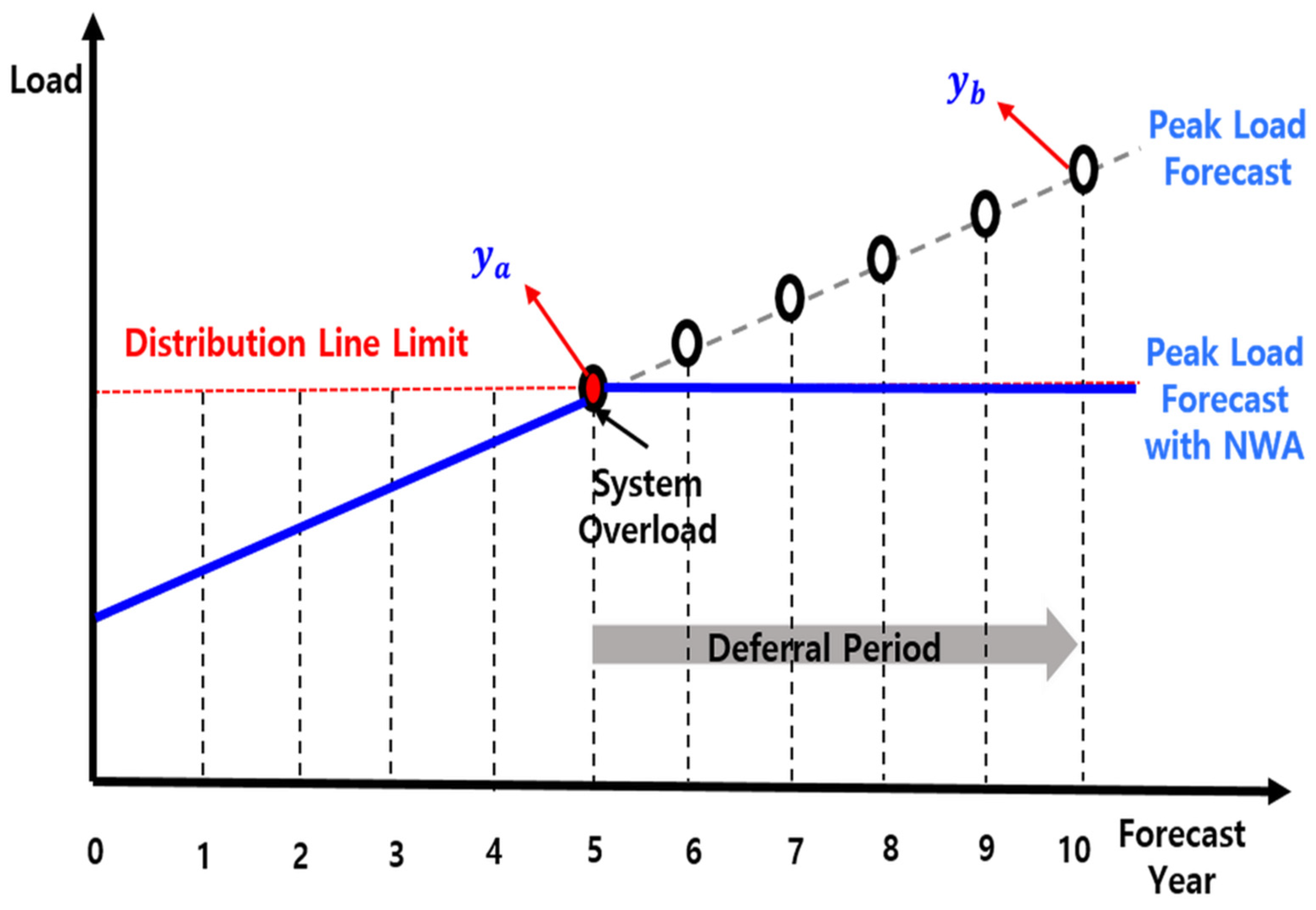
3.3.5. Distribution Line Overload Prevention Constraints
3.4. BCA
4. Case Study
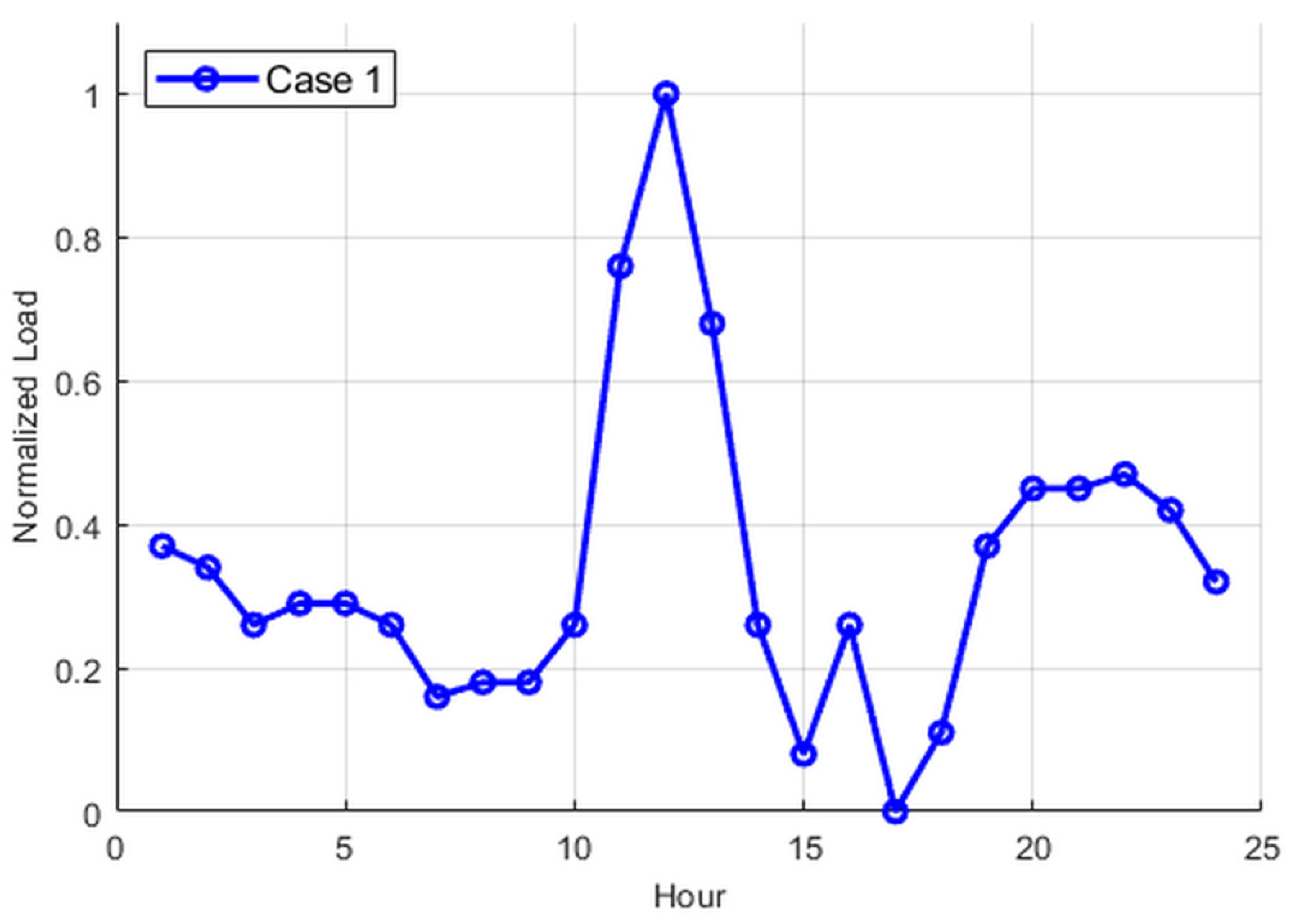
4.1. Load Similarity Analysis
4.2. NWA Portfolio
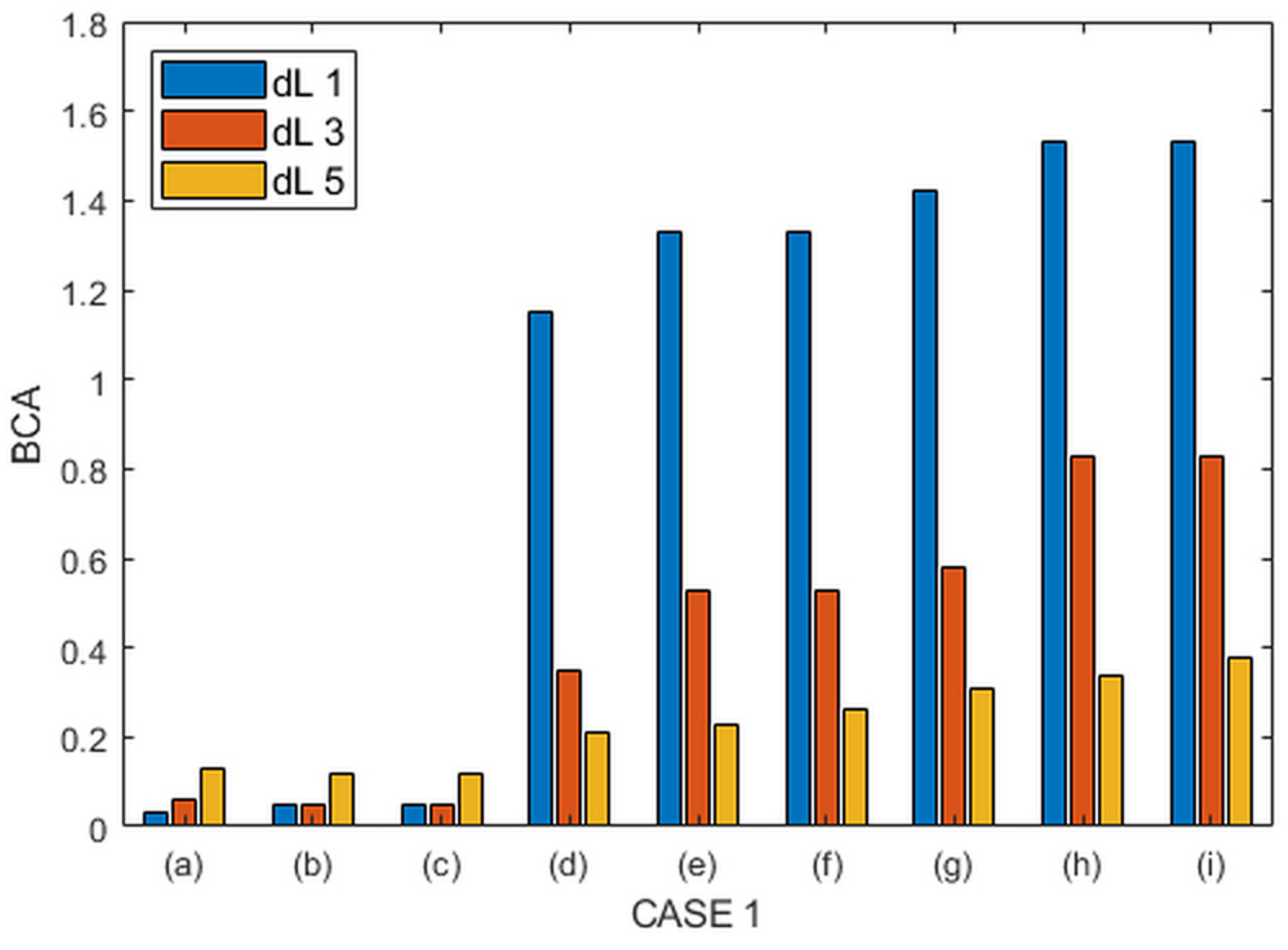
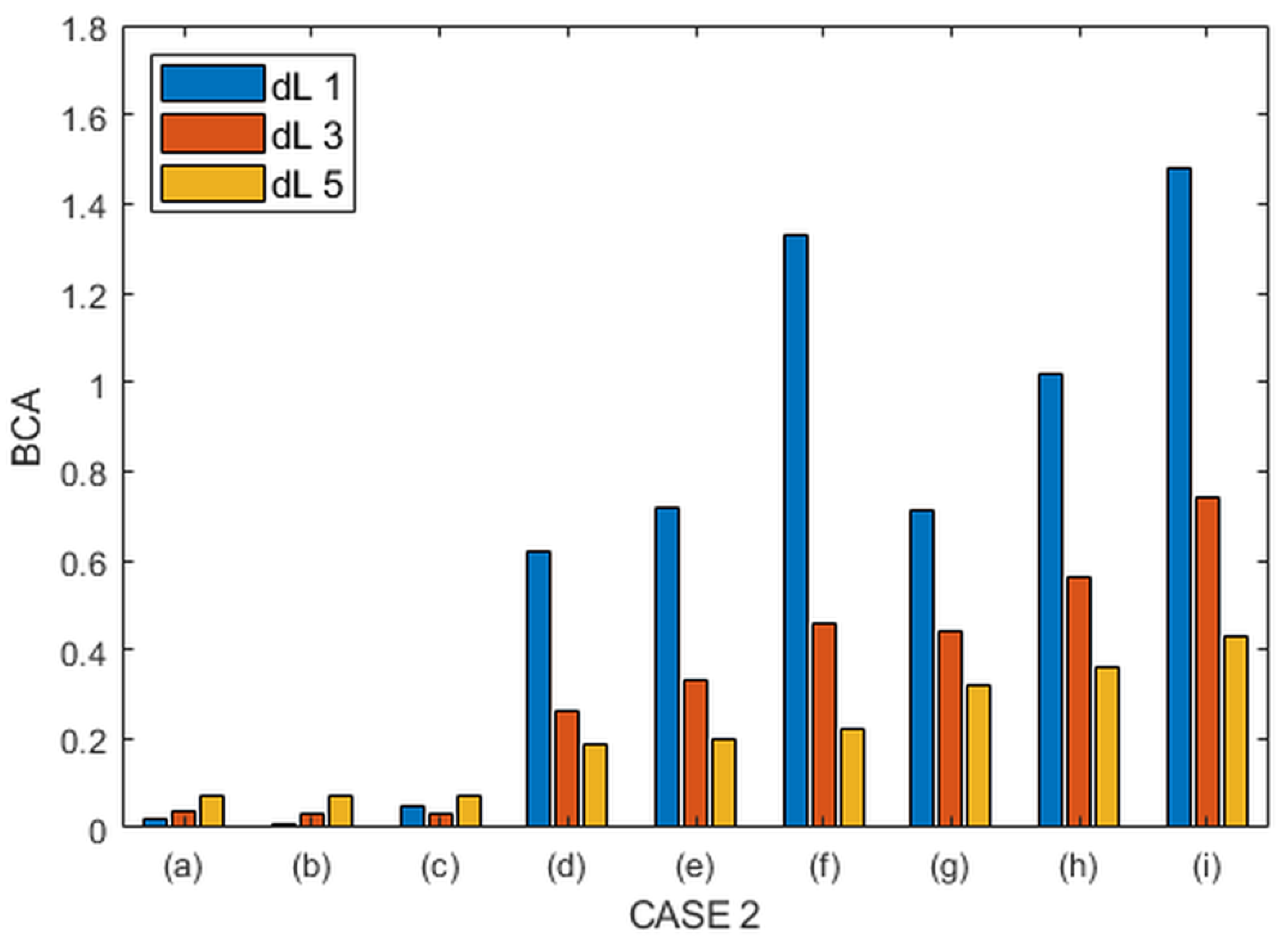
4.3. Numerical Results of BCA
5. Conclusions
Author Contributions
Funding
Data Availability Statement
Acknowledgments
Conflicts of Interest
References
- IEA. Net Zero by 2050: A Roadmap for the Global Energy Sector; International Energy Agency: Paris, France, 2021. [Google Scholar]
- REN21. Renewables 2023 Global Status Report; REN21: Paris, France, 2023. [Google Scholar]
- IPCC. Sixth Assessment Report: Climate Change 2023; Intergovernmental Panel on Climate Change (IPCC): Geneva, Switzerland, 2023. [Google Scholar]
- BloombergNEF. New Energy Outlook 2023; BloombergNEF: New York, NY, USA, 2023. [Google Scholar]
- IRENA. World Energy Transitions Outlook 2023; International Renewable Energy Agency: Abu Dhabi, United Arab Emirate, 2023. [Google Scholar]
- McKinsey & Company. The Future of Power Systems in Energy Transition; McKinsey & Company: New York, NY, USA, 2022. [Google Scholar]
- European Commission. Fit for 55 Package; European Commission: Brussels, Belgium, 2021. [Google Scholar]
- Papaefthymiou, G.; Dragoon, K.; Grunewald, P. Decentralised power systems in transition. Appl. Energy 2021, 286, 116500. [Google Scholar]
- Lund, H.; Østergaard, P.A.; Connolly, D.; Ridjan, I. Smart energy systems for coherent 100% renewable energy and transport solutions. Appl. Energy 2015, 145, 139–154. [Google Scholar]
- Lee, D.; Kim, D.; Joo, S.-K. Interval-stochastic programming for integrated generation, transmission, and energy storage system (ESS) planning considering uncertainty in renewable energy sources. IEEE Access 2025, 13, 30834–30844. [Google Scholar] [CrossRef]
- Korea Energy Agency. Korea Energy Master Plan; Korea Energy Agency: Sejong, Republic of Korea, 2022. [Google Scholar]
- Kim, J.H.; Lee, K.; Park, Y.; Lee, H. Renewable integration in Korea: Challenges and policy implications. Energy Policy 2021, 156, 112447. [Google Scholar]
- Hung, D.Q.; Mithulananthan, N.; Lee, K.Y. Determining PV penetration for distribution systems with time-varying load models. IEEE Trans. Power Syst. 2014, 29, 3048–3057. [Google Scholar] [CrossRef]
- Zhao, H.; Wang, F.; Lin, Y. Economic analysis of large-scale renewable energy source investment incorporating power system transmission costs. Energies 2023, 16, 7407. [Google Scholar]
- CIGRE. Flexibility in Power Systems; Technical Brochure No. 765; CIGRE: Paris, France, 2019. [Google Scholar]
- Kim, S.; Joo, S.-K. Spatiotemporal operation method for mobile virtual power line in power system with mobile energy storage systems. J. Energy Storage 2025, 67, 115196. [Google Scholar] [CrossRef]
- Deb, C.; Zhang, F.; Yang, J.; Lee, S.E.; Shah, K.W. A review on time series forecasting techniques for building energy consumption. Renew. Sustain. Energy Rev. 2017, 74, 902–924. [Google Scholar]
- Lee, D.; Lee, D.; Jang, H.; Joo, S.-K. Backup capacity planning considering short-term variability of renewable energy resources in a power system. Electronics 2021, 10, 709. [Google Scholar] [CrossRef]
- Chicco, G. Overview and performance assessment of the clustering methods for electrical load pattern grouping. Energy 2012, 42, 68–80. [Google Scholar] [CrossRef]
- Moon, G.-H.; Ko, R.; Joo, S.-K. Integration of smart grid resources into generation and transmission planning using an interval-stochastic model. Energies 2020, 13, 1843. [Google Scholar] [CrossRef]
- Convergent Energy & Power. O&R Deploys 12MW/57MWh Battery Systems. In Utility Dive; Convergent Energy & Power: New York, NY, USA, 2023. [Google Scholar]
- NV Energy. 2024 Integrated Resource Plan Summary; NV Public Utilities Commission: Carson City, NV, USA, 2024. [Google Scholar]
- Independent Electricity System Operator (IESO). York Region Non-Wires Alternative Demonstration Final Report; Independent Electricity System Operator: Toronto, ON, Canada, 2024. [Google Scholar]
- ICF. Front-of-Meter Solar and Storage: Economic Potential in EU Markets; ICF International: Fairfax, VA, USA, 2024. [Google Scholar]
- Ministry of Economy, Trade and Industry (METI). Smart Grid Roadmap and Pilot Programs; Agency for Natural Resources and Energy: Tokyo, Japan, 2023.
- Korea Power Exchange. Briefing Material for the Jeju Renewable Energy Bidding Pilot Project; Korea Power Exchange: Naju, Republic of Korea, 2024; Available online: https://www.kpx.or.kr (accessed on 19 June 2025).
- He, L.; Zhang, L.; Xia, Q. A novel load pattern recognition method for residential consumers based on smart meter data. Appl. Energy 2020, 275, 115389. [Google Scholar]
- Contreras-Ocaña, S.; Mancarella, P.; Mancarella, D. A bi-level framework for distributed energy resources planning considering DER owner and system operator decisions. Sustain. Energy Grids Netw. 2019, 18, 100220. [Google Scholar]
- Laws, N.D.; Webber, M.E. Pricing and optimization of distributed energy resources as non-wires alternatives. Appl. Energy 2023, 338, 120962. [Google Scholar]
- Electric Power Research Institute (EPRI). Non-Wires Alternatives: A Planning and Evaluation Guide; EPRI Report 3002018432; EPRI: Palo Alto, CA, USA, 2023. [Google Scholar]
- Bejarano, M.; Ortega, A.; Rey-Stolle, M. Clustering of residential electricity demand curves based on correlation and trend identification. Energy Build. 2017, 149, 78–90. [Google Scholar]
- Kim, J.; Han, S.; Cho, Y. Load classification and estimation for demand response based on smart meter data. IEEE Trans. Smart Grid 2019, 10, 4421–4430. [Google Scholar]
- Zhou, S.; Brown, T. Smart meter data analysis for electricity consumers: Survey, issues and recommendations. IEEE Trans. Ind. Inform. 2019, 15, 1417–1429. [Google Scholar]
- Mirowski, F.M.; Madani, D.; Cvetkovic, M.S. Unsupervised load profiling and customer segmentation. Electr. Power Syst. Res. 2018, 158, 166–174. [Google Scholar]
- Luo, X.; Xie, Z.; Xu, X.; Chen, H. Load profile clustering and classification using smart meter data: A review. Energies 2021, 14, 1083. [Google Scholar]
- Hong, T.; Pinson, P.; Fan, S.; Zareipour, H.; Troccoli, A.; Hyndman, R.J. Probabilistic energy forecasting: Global energy forecasting competition 2014 and beyond. Int. J. Forecast. 2016, 32, 896–913. [Google Scholar] [CrossRef]
- Kwac, H.; Flora, J.; Rajagopal, R. Household load curve clustering using segmentation and prediction. IEEE Trans. Smart Grid 2014, 5, 420–430. [Google Scholar] [CrossRef]
- Kim, H.; Lim, Y.; Oh, H.; Lee, S. Optimal sizing of battery energy storage systems considering capacity degradation. IEEE Trans. Power Syst. 2019, 34, 1567–1575. [Google Scholar]
- Luo, X.; Wang, J.; Dooner, M.; Clarke, J. Overview of current development in electrical energy storage technologies and the application potential in power system operation. Appl. Energy 2015, 137, 511–536. [Google Scholar] [CrossRef]
- Hassan, M.; Mahmood, N.; Sajid, A.A. Comparison of time series similarity measures for load profiling. Int. J. Electr. Power Energy Syst. 2020, 119, 105878. [Google Scholar]
- Fan, C.; Xiao, F.; Wang, S. Development of prediction models for next-day building energy consumption and peak power demand using data mining techniques. Appl. Energy 2014, 127, 1–10. [Google Scholar] [CrossRef]
- Neubauer, J.; Simpson, M.; Wood, E. Energy Storage System Performance Optimization Considering Degradation; National Renewable Energy Laboratory (NREL): Golden, CO, USA, 2016.
- Denholm, P.; Ela, E.; Kirby, B.; Milligan, M. The Role of Energy Storage with Renewable Electricity Generation; National Renewable Energy Laboratory (NREL): Golden, CO, USA, 2010.
- Zhang, Z.; Xu, Y.; Li, F. Flexible operation of battery energy storage system for renewable energy integration and power quality improvement. IET Renew. Power Gener. 2014, 8, 131–140. [Google Scholar]
- Kim, S.; Joo, S.-K. Resilience enhancement method in coupled power and transportation systems with mobile energy resources during hurricanes. IEEE Trans. Ind. Appl. 2025. early access. [Google Scholar]
- De Martini, P.; Kristov, L. Distribution Systems in a High Distributed Energy Resources Future; Lawrence Berkeley National Laboratory: Berkeley, CA, USA, 2015. [Google Scholar]
- EH Pechan & Associates, Inc. The Role of Cost-Benefit Analysis in Environmental Decision-Making; U.S. Environmental Protection Agency: Washington, DC, USA, 2010.
- Scott, M.J.; Sands, R.D. The economics of electric system investment: Theory and application. Energy Econ. 1999, 21, 313–325. [Google Scholar]
- O’Connell, M.; De Martini, P. Non-Wires Alternatives: Case Studies from Across the Country; Rocky Mountain Institute (RMI): Basalt, CO, USA, 2020. [Google Scholar]
- Korea Electric Power Corporation (KEPCO). Standard Unit Prices for Electrical Construction. KEPCO Disclosure Portal. 2024. Available online: https://home.kepco.co.kr/kepco/CO/htmlView/CODCHP001.do?menuCd=FN04040301 (accessed on 19 June 2025).
- Korea Power Exchange (KPX). Daily Weighted Average SMP. EPSIS, Korea Power Exchange. 2024. Available online: https://epsis.kpx.or.kr (accessed on 19 June 2025).
- Korea Power Exchange (KPX). Average SMP by Region—2024. EPSIS. 2024. Available online: https://epsis.kpx.or.kr (accessed on 19 June 2025).
- Korea Energy Agency (KEA). REC Market Statistics 2024. New and Renewable Energy Center. 2024. Available online: https://www.energy.or.kr (accessed on 19 June 2025).
- Yan, G.; Liu, D.; Li, J.; Mu, G. A cost accounting method of the Li-ion battery energy storage system for frequency regulation considering the effect of life degradation. Prot. Control. Mod. Power Syst. 2018, 3, 4. [Google Scholar] [CrossRef]
- Vithayasrichareon, P.; Mills, G.; MacGill, I.F. Impact of electric vehicles and solar PV on future generation portfolio investment. IEEE Trans. Sustain. Energy 2015, 6, 899–908. [Google Scholar] [CrossRef]
- Padmanabhan, N.; Bhattacharya, K. Including demand response and battery energy storage systems in uniform marginal price based electricity markets. IEEE Trans. Power Syst. 2013, 28, 2962–2971. [Google Scholar]

| Type | Components | Values | |
|---|---|---|---|
| Benefit | Distribution system reinforcement | 3,000,268 (USD) | |
| Distribution system O&M | 5004 (USD) | ||
| ESS charge/discharge revenue | 0.06 (USD/kWh) | ||
| PV generation revenue | 0.1 (USD/kWh) | ||
| PV renewable energy certificate (REC) | 514.1 (USD/REC) | ||
| Cost | ESS installation (PCS) | 145.3 (USD/kW) | |
| ESS installation (SOC) | 273.2 (USD/kW) | ||
| PV installation | 877 (USD/kW) | ||
| ESS O&M | 3.5 (USD/kW) | ||
| PV O&M | 13.7 (USD/kW) | ||
| DR incentive | 0.07 (USD/kWh) | ||
| Type | Components | Values | |
|---|---|---|---|
| Case 1 | Commercial characteristic coefficient | 0.398 | |
| Residential characteristic coefficient | 0.345 | ||
| Industrial characteristic coefficient | 0.330 | ||
| Case 2 | Commercial characteristic coefficient | 0.369 | |
| Residential characteristic coefficient | 0.486 | ||
| Industrial characteristic coefficient | 0.287 | ||
| Case 3 | Commercial characteristic coefficient | 0.565 | |
| Residential characteristic coefficient | 0.374 | ||
| Industrial characteristic coefficient | 0.502 | ||
| NWA Portfolio | |||||||
|---|---|---|---|---|---|---|---|
| Overall Load Growth ) | 1% | 3% | 5% | ||||
| NWA Resources (MW) | PV | DR | PV | DR | PV | DR | |
| Case 1 | (a) | 0 | 0 | 0 | 0 | 0 | 0 |
| (b) | 0 | 1 | 0 | 1 | 0 | 1 | |
| (c) | 0 | 2 | 0 | 2 | 0 | 2 | |
| (d) | 1 | 0 | 1 | 0 | 1 | 0 | |
| (e) | 1 | 1 | 1 | 1 | 1 | 1 | |
| (f) | 1 | 2 | 1 | 2 | 1 | 2 | |
| (g) | 2 | 0 | 2 | 0 | 2 | 0 | |
| (h) | 2 | 1 | 2 | 1 | 2 | 1 | |
| (i) | 2 | 2 | 2 | 2 | 2 | 2 | |
| Case 2 | (a) | 0 | 0 | 0 | 0 | 0 | 0 |
| (b) | 0 | 1 | 0 | 1 | 0 | 1 | |
| (c) | 0 | 2 | 0 | 2 | 0 | 2 | |
| (d) | 1 | 0 | 1 | 0 | 1 | 0 | |
| (e) | 1 | 1 | 1 | 1 | 1 | 1 | |
| (f) | 1 | 2 | 1 | 2 | 1 | 2 | |
| (g) | 2 | 0 | 2 | 0 | 2 | 0 | |
| (h) | 2 | 1 | 2 | 1 | 2 | 1 | |
| (i) | 2 | 2 | 2 | 2 | 2 | 2 | |
| Case 3 | (a) | 0 | 0 | 0 | 0 | 0 | 0 |
| (b) | 0 | 1 | 0 | 1 | 0 | 1 | |
| (c) | 0 | 2 | 0 | 2 | 0 | 2 | |
| (d) | 1 | 0 | 1 | 0 | 1 | 0 | |
| (e) | 1 | 1 | 1 | 1 | 1 | 1 | |
| (f) | 1 | 2 | 1 | 2 | 1 | 2 | |
| (g) | 2 | 0 | 2 | 0 | 2 | 0 | |
| (h) | 2 | 1 | 2 | 1 | 2 | 1 | |
| (i) | 2 | 2 | 2 | 2 | 2 | 2 | |
| Type | ESS PCS (MW) | ESS SOC (MWh) | Total Charging (MWh) | |
|---|---|---|---|---|
| Case 1 | (a) | 1.2 | 1.6 | 18.1 |
| (b) | 0.3 | 0.4 | 0.6 | |
| (c) | 0.3 | 0.4 | 0.6 | |
| (d) | 0.6 | 0.8 | 7.9 | |
| (e) | 0.2 | 0.4 | 0.3 | |
| (f) | 0.2 | 0.4 | 0.3 | |
| (g) | 0.4 | 0.6 | 4 | |
| (h) | 0.1 | 0.2 | 0.1 | |
| (i) | 0.1 | 0.2 | 0.1 | |
| Case 2 | (a) | 2.4 | 7.2 | 86 |
| (b) | 1.3 | 3.2 | 15.3 | |
| (c) | 0.2 | 0.4 | 0.44 | |
| (d) | 2.4 | 7 | 66.4 | |
| (e) | 1.3 | 3 | 14.7 | |
| (f) | 0.2 | 0.4 | 0.28 | |
| (g) | 2.4 | 6.8 | 59.2 | |
| (h) | 1.3 | 3 | 14.2 | |
| (i) | 0.2 | 0.4 | 0.44 | |
| Case 3 | (a) | 1 | 6.8 | 56.8 |
| (b) | 1 | 2.6 | 15.1 | |
| (c) | 1 | 2.4 | 15.1 | |
| (d) | 0.4 | 1.8 | 6.1 | |
| (e) | 0.2 | 0.4 | 0.8 | |
| (f) | 0.2 | 0.4 | 0.8 | |
| (g) | 0.1 | 0.2 | 0.18 | |
| (h) | 0 | 0 | 0 | |
| (i) | 0 | 0 | 0 | |
| Type | ESS PCS (MW) | ESS SOC (MWh) | Total Charging (MWh) | |
|---|---|---|---|---|
| Case 1 | (a) | 3 | 11.8 | 475.6 |
| (b) | 2 | 6.4 | 241.6 | |
| (c) | 2 | 6.4 | 202.3 | |
| (d) | 2.4 | 11.2 | 353.1 | |
| (e) | 1.6 | 5.8 | 153.9 | |
| (f) | 1.6 | 5.6 | 126.2 | |
| (g) | 2.3 | 10.8 | 289.5 | |
| (h) | 1.5 | 5.4 | 114.6 | |
| (i) | 1.5 | 5.4 | 92.8 | |
| Case 2 | (a) | 4.6 | 16.8 | 515.3 |
| (b) | 3.5 | 11.4 | 219.5 | |
| (c) | 2.4 | 7.8 | 126.9 | |
| (d) | 4.6 | 16.4 | 448.1 | |
| (e) | 3.5 | 10.8 | 175.9 | |
| (f) | 2.4 | 6.6 | 97 | |
| (g) | 4.6 | 16 | 404.6 | |
| (h) | 3.5 | 10.6 | 154.6 | |
| (i) | 2.3 | 6.4 | 85.3 | |
| Case 3 | (a) | 3.1 | 37.2 | 1212 |
| (b) | 2.8 | 26.2 | 866 | |
| (c) | 2.8 | 20.6 | 768.1 | |
| (d) | 2.5 | 25 | 643.9 | |
| (e) | 2 | 19 | 424.8 | |
| (f) | 2 | 14 | 390.6 | |
| (g) | 2 | 18.6 | 321.8 | |
| (h) | 1.7 | 13.2 | 197.7 | |
| (i) | 1.7 | 9.6 | 186.6 | |
| Type | ESS PCS (MW) | ESS SOC (MWh) | Total Charging (MWh) | |
|---|---|---|---|---|
| Case 1 | (a) | 5 | 38.2 | 3294 |
| (b) | 3.9 | 32.6 | 2718 | |
| (c) | 3.7 | 30.8 | 2488 | |
| (d) | 4.6 | 37 | 2535 | |
| (e) | 3.6 | 31.4 | 2150 | |
| (f) | 3.6 | 26.2 | 1940 | |
| (g) | 4.5 | 35.8 | 2146 | |
| (h) | 3.8 | 30.2 | 1780 | |
| (i) | 3.8 | 25 | 1585 | |
| Case 2 | (a) | 7.1 | 41.6 | 2079 |
| (b) | 5.9 | 36 | 1632 | |
| (c) | 4.8 | 30.8 | 1357 | |
| (d) | 7 | 35 | 1854 | |
| (e) | 5.9 | 29.4 | 1424 | |
| (f) | 4.8 | 24.6 | 1165 | |
| (g) | 7 | 29.8 | 1701 | |
| (h) | 5.9 | 24.2 | 1289 | |
| (i) | 4.8 | 18.6 | 1045 | |
| Case 3 | (a) | 5.4 | 190.6 | 4915 |
| (b) | 4.9 | 162.8 | 4429 | |
| (c) | 4.9 | 135.2 | 4105 | |
| (d) | 4.8 | 162.4 | 3647 | |
| (e) | 4.4 | 134.6 | 3238 | |
| (f) | 4.4 | 107 | 2988 | |
| (g) | 4.3 | 134.2 | 2705 | |
| (h) | 3.8 | 112 | 2364 | |
| (i) | 3.8 | 90 | 2178 | |
| Type | BCA | |||||||||
|---|---|---|---|---|---|---|---|---|---|---|
| (a) | (b) | (c) | (d) | (e) | (f) | (g) | (h) | (i) | ||
| Case 1 | 1 | 0.03 | 0.05 | 0.05 | 1.15 | 1.33 | 1.33 | 1.42 | 1.53 | 1.53 |
| 3 | 0.06 | 0.05 | 0.05 | 0.35 | 0.53 | 0.53 | 0.58 | 0.83 | 0.83 | |
| 5 | 0.13 | 0.12 | 0.12 | 0.21 | 0.23 | 0.26 | 0.31 | 0.34 | 0.38 | |
| Case 2 | 1 | 0.02 | 0.01 | 0.05 | 0.62 | 0.72 | 1.33 | 0.71 | 1.02 | 1.48 |
| 3 | 0.04 | 0.03 | 0.03 | 0.26 | 0.33 | 0.46 | 0.44 | 0.56 | 0.74 | |
| 5 | 0.07 | 0.07 | 0.07 | 0.19 | 0.2 | 0.22 | 0.32 | 0.36 | 0.43 | |
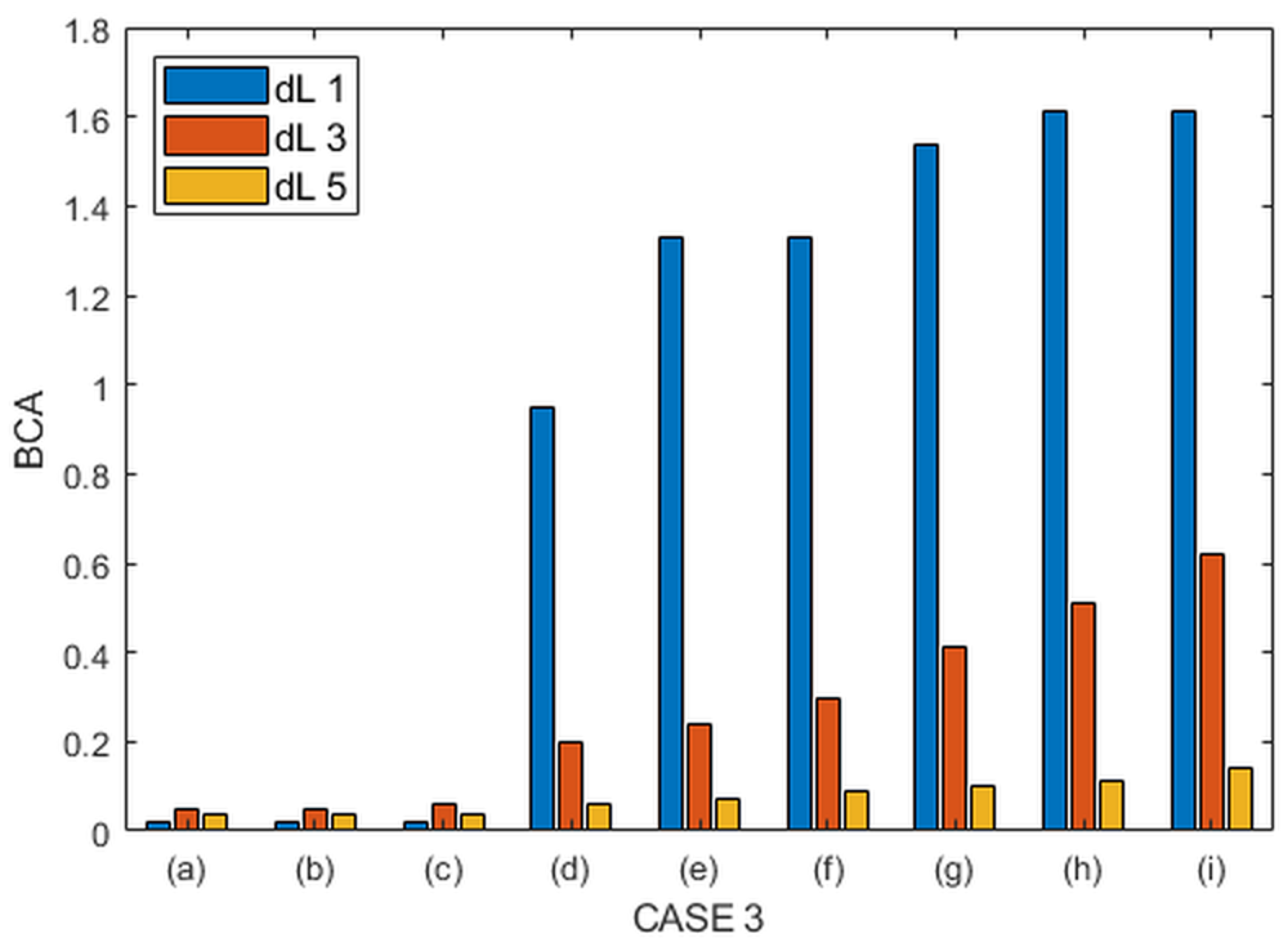
| Case 3 | 1 | 0.02 | 0.02 | 0.02 | 0.95 | 1.33 | 1.33 | 1.54 | 1.61 | 1.61 |
| 3 | 0.05 | 0.05 | 0.06 | 0.2 | 0.24 | 0.3 | 0.41 | 0.51 | 0.62 | |
| 5 | 0.04 | 0.04 | 0.04 | 0.06 | 0.07 | 0.09 | 0.1 | 0.11 | 0.14 | |
| Type | Values | ||||||||
|---|---|---|---|---|---|---|---|---|---|
| Scenario (i) in Case 1 | Scenario (i) in Case 2 | Scenario (i) in Case 3 | |||||||
| DR Rate 80% | DR Rate 100% | DR Rate 120% | DR Rate 80% | DR Rate 100% | DR Rate 120% | DR Rate 80% | DR Rate 100% | DR Rate 120% | |
| ESS PCS (MW) | 1.5 | 1.5 | 1.5 | 2.8 | 2.3 | 1.9 | 1.7 | 1.7 | 1.7 |
| ESS SOC (MWh) | 5.4 | 5.4 | 5.4 | 8.2 | 6.4 | 5 | 10.6 | 9.6 | 8.4 |
| Total Charging (MWh) | 94.4 | 92.8 | 92.7 | 100.3 | 85.3 | 77.4 | 187.1 | 186.6 | 186.5 |
| BCA | 0.83 | 0.83 | 0.83 | 0.65 | 0.74 | 0.83 | 0.59 | 0.62 | 0.67 |
| Type | R | BCA | ||||||||
|---|---|---|---|---|---|---|---|---|---|---|
| (a) | (b) | (c) | (d) | (e) | (f) | (g) | (h) | (i) | ||
| Case 1 | 3 | 0.06 | 0.06 | 0.05 | 0.39 | 0.58 | 0.59 | 0.64 | 0.91 | 0.91 |
| 5 | 0.06 | 0.05 | 0.05 | 0.35 | 0.53 | 0.53 | 0.58 | 0.83 | 0.83 | |
| 7 | 0.05 | 0.05 | 0.04 | 0.32 | 0.48 | 0.48 | 0.53 | 0.75 | 0.75 | |
| Case 2 | 3 | 0.05 | 0.03 | 0.03 | 0.28 | 0.36 | 0.51 | 0.48 | 0.61 | 0.82 |
| 5 | 0.04 | 0.03 | 0.03 | 0.26 | 0.33 | 0.46 | 0.44 | 0.56 | 0.74 | |
| 7 | 0.04 | 0.03 | 0.02 | 0.23 | 0.3 | 0.42 | 0.4 | 0.51 | 0.67 | |
| Case 3 | 3 | 0.06 | 0.06 | 0.06 | 0.22 | 0.27 | 0.34 | 0.46 | 0.57 | 0.69 |
| 5 | 0.05 | 0.05 | 0.06 | 0.2 | 0.24 | 0.3 | 0.41 | 0.51 | 0.62 | |
| 7 | 0.05 | 0.05 | 0.05 | 0.18 | 0.22 | 0.28 | 0.38 | 0.47 | 0.57 | |
| Type | Values | |||||
|---|---|---|---|---|---|---|
| Case 1 | Case 2 | Case 3 | ||||
| (a) | (c) | (a) | (c) | (a) | (c) | |
| ESS PCS (MW) | 3 | 2 | 4.6 | 2.4 | 3.1 | 2.8 |
| ESS SOC (MWh) | 11.8 | 6.4 | 16.8 | 7.8 | 37.2 | 20.6 |
| Total Charging (MWh) | 475.6 | 202.3 | 515.3 | 126.9 | 1212 | 768.1 |
| BCA | 0.06 | 0.05 | 0.04 | 0.03 | 0.05 | 0.06 |
| Type | Values | |||||
|---|---|---|---|---|---|---|
| Case 1 | Case 2 | Case 3 | ||||
| (a) | (g) | (a) | (g) | (a) | (g) | |
| ESS PCS (MW) | 3 | 2.3 | 4.6 | 4.6 | 3.1 | 2 |
| ESS SOC (MWh) | 11.8 | 10.8 | 16.8 | 16 | 37.2 | 18.6 |
| Total Charging (MWh) | 475.6 | 289.5 | 515.3 | 404.6 | 1212 | 190.6 |
| BCA | 0.06 | 0.58 | 0.04 | 0.44 | 0.05 | 0.41 |
Disclaimer/Publisher’s Note: The statements, opinions and data contained in all publications are solely those of the individual author(s) and contributor(s) and not of MDPI and/or the editor(s). MDPI and/or the editor(s) disclaim responsibility for any injury to people or property resulting from any ideas, methods, instructions or products referred to in the content. |
© 2025 by the authors. Licensee MDPI, Basel, Switzerland. This article is an open access article distributed under the terms and conditions of the Creative Commons Attribution (CC BY) license (https://creativecommons.org/licenses/by/4.0/).
Share and Cite
Park, J.; Joo, S.-K. Techno-Economic Analysis of Non-Wire Alternative (NWA) Portfolios Integrating Energy Storage Systems (ESS) with Photovoltaics (PV) or Demand Response (DR) Resources Across Various Load Profiles. Energies 2025, 18, 3568. https://doi.org/10.3390/en18133568
Park J, Joo S-K. Techno-Economic Analysis of Non-Wire Alternative (NWA) Portfolios Integrating Energy Storage Systems (ESS) with Photovoltaics (PV) or Demand Response (DR) Resources Across Various Load Profiles. Energies. 2025; 18(13):3568. https://doi.org/10.3390/en18133568
Chicago/Turabian StylePark, Juwon, and Sung-Kwan Joo. 2025. "Techno-Economic Analysis of Non-Wire Alternative (NWA) Portfolios Integrating Energy Storage Systems (ESS) with Photovoltaics (PV) or Demand Response (DR) Resources Across Various Load Profiles" Energies 18, no. 13: 3568. https://doi.org/10.3390/en18133568
APA StylePark, J., & Joo, S.-K. (2025). Techno-Economic Analysis of Non-Wire Alternative (NWA) Portfolios Integrating Energy Storage Systems (ESS) with Photovoltaics (PV) or Demand Response (DR) Resources Across Various Load Profiles. Energies, 18(13), 3568. https://doi.org/10.3390/en18133568