Abstract
To enhance the operational stability of distribution networks during peak periods, this paper proposes a multi-timescale operational method considering load forecasting impacts. Firstly, the Crested Porcupine Optimizer (CPO) is employed to optimize the hyperparameters of long short-term memory (LSTM) networks for an accurate prediction of the next-day load curves. Building on this foundation, a multi-timescale optimization strategy is developed: During the day-ahead operation phase, a conservation voltage reduction (CVR)-based regulation plan is formulated to coordinate the control of on-load tap changers (OLTCs) and distributed resources, alleviating peak-shaving pressure on the upstream grid. In the intraday optimization phase, real-time adjustments of OLTC tap positions are implemented to address potential voltage violations, accompanied by an electrical distance-based control strategy for flexible adjustable resources, enabling rapid voltage recovery and enhancing system stability and robustness. Finally, a modified IEEE-33 node system is adopted to verify the effectiveness of the proposed multi-timescale operational method. The method demonstrates a load forecasting accuracy of 93.22%, achieves a reduction of 1.906% in load power demand, and enables timely voltage regulation during intraday limit violations, effectively maintaining grid operational stability.
1. Introduction
With the acceleration of global warming and urbanization, air conditioning loads have been accounting for an increasingly significant proportion of electricity consumption [1,2]. The concentrated usage periods and significant load fluctuations characteristic of air conditioning loads pose new challenges to accurate grid load forecasting and efficient energy utilization. The surge in electricity demand during summer heat waves not only widens the peak-valley load difference but may also trigger voltage instability and power supply shortages [3,4]. Therefore, accurate load curve prediction and subsequent distribution network optimization strategies are crucial for improving energy efficiency and ensuring grid operational safety.
Load forecasting remains a critical component in power system operation and management [5]. Traditional methods include regression analysis [6], Kalman filtering [7], and time-series analysis [8]. With recent advancements in artificial intelligence, intelligent forecasting techniques such as fuzzy logic, support vector machines (SVMs) [9], random forests [10], and neural networks [11] have demonstrated superior capability in handling temporal dependencies and nonlinear characteristics of load data, significantly enhancing prediction accuracy. However, these methods exhibit limitations: SVMs struggle with large-scale datasets due to prolonged training time, compromising real-time performance, while neural networks frequently suffer from slow convergence and overfitting caused by improper parameterization [12]. Recent studies have proposed optimization algorithms to refine neural network parameters, determining optimal network topology and hyperparameters to enhance forecasting precision [13]. Notably, PSO-optimized LSTM (PSO-LSTM) has shown promise in load forecasting [14], yet it still faces two key challenges: (1) premature convergence to suboptimal solutions when handling multi-modal load patterns and (2) inadequate adaptation to abrupt load changes caused by extreme weather or EV charging events [15]. These limitations motivate the development of more advanced bio-inspired optimization techniques that can better balance global exploration and local exploitation in the hyperparameter space while maintaining computational efficiency.
Following daily load curve prediction, conservation voltage reduction (CVR) technology [16] has emerged as an effective approach to reducing peak load demand and maintaining grid stability. With origins tracing back to 1973 pilot projects in Europe and North America [17], CVR has demonstrated proven efficacy through decades of utility-scale implementations. The technology operates within permissible voltage deviation ranges (0.94–1.0 p.u.) by strategically adjusting supply voltages, and early trials achieved 4% load reduction with 5% voltage reduction [18]. Subsequent deployments by leading utilities like Southern California Edison and Bonneville Power Authority further validate its dual benefits in peak clipping and reactive power management [19,20,21]. Current research has extensively explored CVR applications: The authors of [22] detailed its implementation in peak shaving and energy conservation. The authors of [23,24,25] developed optimization models integrating CVR with automatic voltage control for coordinated load reduction. Another study [26] combined on-load tap changer (OLTC) adjustments with network reconfiguration and distributed energy resource coordination to optimize voltage profiles. In addition, a CVR optimization framework balancing grid security and market dynamics was proposed in [27,28], which established an energy-minimization model for CVR operation in renewable-rich grids, demonstrating a 0.3–1% load reduction per 1% voltage decrease.
While CVR technology has demonstrated significant load reduction capabilities, its voltage-lowering effect creates operational challenges. When day-ahead load forecasts deviate substantially from actual intraday loads—particularly during extreme weather events or unexpected demand surges—the system’s reduced voltage margins may lead to limit violations. This necessitates coordinated multi-timescale control strategies. Existing approaches [29,30] have explored the synergistic regulation of passive resources (OLTCs and CBs) with active resources (DERs and ESS) across different timescales to optimize renewable energy integration. However, these methods fail to account for CVR-specific conditions: (1) node loads exhibit voltage-dependent characteristics according to ZIP models, (2) system voltages persistently operate near their lower bounds (0.94–1.0 p.u.), and (3) traditional corrective actions may inadvertently counteract the CVR effect’s energy-saving benefits.
Based on the above discussion, this paper proposes a multi-timescale operational method considering load forecasting impacts. The main contributions of this paper are as follows:
(1) A CPO-LSTM hybrid load forecasting method is proposed, where the Crested Porcupine Optimizer (CPO) algorithm optimizes hyperparameters of long short-term memory (LSTM) networks, enabling the effective prediction of next-day load curves in distribution networks with 93.22% accuracy.
(2) A multi-timescale optimization strategy is developed, formulating CVR-based dispatch plans in the day-ahead phase and implementing real-time voltage monitoring with coordinated control of distributed resources during intraday operations, achieving a 1.906% reduction in daily energy consumption while ensuring grid stability.
(3) An OLTC tap-position real-time adjustment mechanism is designed to address voltage violations, complemented by an electrical distance-based flexible resource control strategy for rapid voltage recovery, significantly enhancing system stability and robustness under contingency conditions.
The remainder of this article is organized as follows: The CPO-LSTM load forecasting framework with hyperparameter optimization mechanisms is developed in Section 2. Section 3 introduces conservation voltage reduction (CVR) technology and explains its energy-saving potential analysis. Then, the architecture of the multi-timescale optimization strategy integrating day-ahead and intraday coordination is discussed in Section 4. Section 5 provides the simulation analysis to validate the methodology’s effectiveness, and the conclusion is given in Section 6.
2. CPO-LSTM-Based Power Load Forecasting
2.1. LSTM Model
Long short-term memory (LSTM) is a specialized type of recurrent neural network (RNN) designed for processing sequential and time-series data. Compared to traditional RNNs, LSTM exhibits superior memory retention and long-term dependency modeling capabilities. Its core innovation lies in the memory cell structure, which stores and manages long-term information through a cell state vector regulated by three gating mechanisms: the input gate, the forget gate, and the output gate.
In LSTM, each timestep’s input comprises three components: the current input vector, the hidden state from the previous timestep, and the cell state (i.e., memory). Specifically, at time t, the input xt is a multi-feature vector containing temporal and spatial characteristics; the hidden state ht−1 is the output from time t−1; and the cell state ct−1 is the memory inherited from time t−1. The following values are computed based on these inputs and previous states:
(1) Input gate activation it:
(2) Forget gate activation ft:
(3) Cell state modulation :
(4) Cell state update ct:
(5) Output gate activation :
(6) Hidden state update :
where Wix, Wih, Wfx, Wfh, Wcx, Wch, Wox, Woh, bi, bf, bc, and bo are the parameters of the LSTM, σ denotes the sigmoid activation function, and ⊙ represents the element-wise multiplication operation.
Through this iterative process, the output of the LSTM unit at each timestep can be computed sequentially. By capturing temporal patterns and dependencies in time-series data through this mechanism, LSTM is effectively applied to short-term power load forecasting in grid systems.
2.2. CPO Optimization Algorithm
The CPO algorithm mimics four defensive strategies of crested porcupines against predators: visual intimidation, acoustic intimidation, chemical attack, and physical defense. Each strategy corresponds to specific search/movement rules for updating candidate solutions, ultimately determining the optimal solution. The algorithmic workflow is as follows:
(1) Visual intimidation: Porcupines deter predators by displaying vivid coloration and quills. In CPO, this is conceptualized as a large-scale movement toward the optimal solution with random perturbations to enhance population diversity:
where y is the average of the current solution and the random solution, Xi is the current solution, Xrand is the random solution, r is the random number between 0 and 1, and Gb_sol is the global optimal solution.
(2) Acoustic intimidation: The crested porcupine makes warning sounds to scare away potential dangers. In the algorithm, it can be regarded as a small adjustment of individual position to maintain population stability and avoid falling into local optimal. The specific algorithm is as follows:
where U1 is a random matrix between 0 and 1, and Xrand1 and Xrand2 are random solutions.
(3) Chemical attack: Gas emission is translated into inter-solution information exchange for exploring new solution spaces:
where St is the strategy factor, fitness (i) is the fitness of the current individual, θ is a small value to avoid zero-division errors, S is the search intensity, and Yt is the time attenuation factor.
(4) Physical defense: The crested porcupines use thorns as a last resort of defense, which, in optimization algorithms, can represent strict protection of the current best solution while exploring other solutions; the specific formula is set as follows:
where Mt is the strategy factor, Ft is the search direction, S is the search intensity, α is the parameter controlling the search intensity, and U2 is a random matrix between 0 and 1.
2.3. Power Load Forecasting Model Based on CPO-LSTM
This study employs the CPO algorithm to optimize three critical hyperparameters of LSTM neural networks, namely the topology structure, iteration count, and learning rate, thereby determining optimal configurations for wind power load forecasting. The CPO-LSTM-based power load prediction process is shown in Figure 1, with the following specific modeling steps:
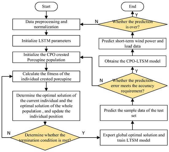
Figure 1.
The process of power load forecasting based on CPO-LSTM.
Step 1: Normalize the data: In order to avoid the dominant role of some characteristics in the optimization process and make the optimization fairer and more accurate, normalize the collected wind power load data and divide them into training sets and test sets.
Step 2: Initialize model parameters: Construct the LSTM architecture by defining hyperparameters, including hidden layer dimensions and learning rate. Establish the CPO framework by configuring population size, search space dimensions, and maximum iterations, and perform the stochastic initialization of particle position vectors.
Step 3: Evaluate fitness: Map each particle’s position vector to LSTM configuration parameters for network training. Utilize the root mean square error (RMSE) as the fitness metric to determine the prediction accuracy of parameter combinations.
Step 4: Update individual locations: Update personal historical best positions and global optimal solutions based on fitness evaluation. Implement spatial exploration–exploitation balance through position updating Formulas (7)–(10).
Step 5: Perform iterative optimization: Execute Steps (3)–(4) cyclically until meeting convergence criteria or reaching maximum generations, thereby obtaining optimal network parameters.
Step 6: Perform model validation and refinement: Integrate optimized parameters into LSTM for final modeling. Assess generalization capability using the validation dataset. Trigger parameter recalibration mechanism when the prediction error exceeds the tolerance threshold, reiterating Steps (2)–(5) until performance specifications are satisfied.
Step 7: Perform sequential prediction and task switching: Deploy the trained CPO-LSTM to generate short-term forecasts for the current data type (wind or load). Switch to the next data type’s training set, repeating Steps 1–6 until all required predictions (wind + load) are completed.
3. CVR Technology and Its Energy-Saving Benefit Analysis
On the basis of load forecasting, CVR technology is further adopted to reduce system energy consumption and maintain the stable operation of the power grid. CVR reduces the total power demand of the system by reducing the voltage of the distribution network, and its implementation effect can be measured by the CVR factor fCVR. fCVR is defined as the ratio of the total system power demand reduction percentage ΔP% to the distribution network voltage reduction percentage ΔU%, which is calculated using Equation (11):
The total power demand of the power system is usually composed of the power demand of the user and the network loss. In the face of different types of load, the voltage adjustment will have different effects on the total power demand of the system. Therefore, fCVR is closely related to load types and load models. In general, the ZIP model can be used to describe the effects of CVR technology on different loads, which can be described by Equation (12) [26], where , are, respectively, the load active and reactive power of node i at time t after CVR measures are taken. Pi,t, Qi,t are, respectively, the load active power and reactive power of node i before CVR measures are taken. , , and are the ZIP load proportion coefficients of node i. Vi,t is the voltage of node i after voltage regulation, and Vi,0 is the voltage of node i before voltage regulation.
It can be seen from (12) that the active and reactive power of the load are composed of three parts. For pure resistive load, reducing the voltage of the network will reduce the current flowing through the load, thus reducing the loss of the load itself and the line loss. By contrast, when the load is a constant power characteristic, although the power is kept constant when the voltage is reduced, the current will inevitably increase, which will lead to an increase in line loss, and then the total energy demand of the system will rise. For constant current characteristic loads, the reduction in voltage does not affect the current flowing through the load, so the power demand of the load decreases, while the line loss remains unchanged, which helps to reduce the total power demand of the entire system. Studies have shown that, in most practical cases, when the voltage is reduced within the allowable range, the increase in line loss caused by constant power load is usually far less than the energy consumption reduced by pure resistive load [31].
Therefore, CVR technology is adopted in the day-ahead dispatching stage in this paper. On the premise of not exceeding the voltage limit and ensuring the safety of equipment, the overall power consumption of the grid is reduced by adjusting the electricity voltage to the low range of the standard voltage, and effective energy saving is promoted. It is worth noting that when formulating the day-ahead scheduling strategy of the distribution network considering CVR, the grid voltage is generally reduced by adjusting the OLTC gear. Due to the long distance of some feeders, the line voltage loss is large, the terminal node voltage is low, and the adjustment range of CVR is limited. In order to ensure that the end voltage of such feeders meets the requirements of power supply quality, reactive power compensation devices can be deployed at a few key nodes of the line.
4. Multi-Time Scale Operation Strategy
Based on the prediction of the next-day load of the distribution system, a flexible resource multi-time scale control technology of the distribution network under the framework of voltage–load regulation is proposed in this paper. In the day-ahead dispatching stage, aiming at the minimum daily energy consumption of the distribution network, the regulation plan of OLTCs and distributed resources is formulated to reduce the total power demand of the system. In the intraday operation stage, when the voltage of the distribution network exceeds the limit, the OLTC gear position is adjusted, while flexible resources are dispatched based on their electrical distance—prioritizing those with the strongest coupling to the affected nodes. This approach ensures both fast voltage recovery and minimal control effort.
4.1. Day-Ahead Optimization of Operation Policies
When the power grid voltage margin is sufficient, the use of CVR technology can reduce the load demand without increasing the extra investment cost and improve the economy and stability of the system operation. Therefore, in this study, a day-ahead optimal scheduling model is designed based on the concept of CVR, which takes the minimum energy used by the distribution network throughout the day as the optimization goal and solves the optimal adjustment gear of OLTC and distributed resource output. The details are as follows:
The objective function is set as follows:
where ΩL is the branch set, ΩN is the node set, rij is the resistance in branch (i, j), Iij,t is the current flowing into branch (i, j) at time t, and is the load power of each node after CVR measures are taken.
Constraints include the following:
(1) System forward push-back power flow constraints:
where Ψb is the network branch set with j as the first end; Pj,k is the first active power of the branch (j, k); PL,j is the load active power of node j; Ψc is the network branch set with j as the end; Pi,j is the first active power of the branch (i, j); Qi,j is the first reactive power of the branch (i, j); ri,j is the resistance of the branch (i, j); Vi and Vj are the actual voltage between node i and node j; PDG,j is the active power emitted by DG of node j; Qj,k is the reactive power of the first segment with j as branch (j, k); QL,j is the reactive power of node j load; xi,j is the reactance of branch (i, j); and QDG is the reactive power emitted by DG of node j.
(2) Node voltage and branch current constraints:
where Vimin and Vimax are, respectively, the upper and lower limits of the voltage of node i; Iij is the current of the branch (i, j); and Iijmin and Iijmax are, respectively, the upper and lower limits of the current of each branch.
(3) Constraint on the output of distributed resources:
where PDG,i is the output power of DG of the i-th node; , and is the upper and lower limits of active power emitted by DG of each node; and is the upper and lower limits of reactive power emitted by DG of each node.
(4) Reactive power compensation device constraints:
where QC,m is the compensation amount of the reactive power compensation device at node m, and and is the minimum and maximum compensation capacity of the reactive power compensation device at node m.
(5) OLTC regulation constraints:
where Vss,1 is the substation voltage after OLTC regulation, Vss,0 is the substation voltage before OLTC regulation, λ is the OLTC regulation gear, ω is the OLTC regulation voltage at each gear, λmin and λmax are the upper and lower limits of OLTC regulation gear, ξλ is the number of OLTC regulation, and ξmax is the maximum number of OLTC regulation.
4.2. Intraday Optimal Operation Strategy to Prevent Voltage Overruns
In the real-time monitoring of the intraday operation of the distribution network, once the node voltage is detected to exceed the limit, the day-ahead dispatching strategy will no longer be applicable. At this point, it is necessary to adjust the OLTC gear and the output of distributed resources to achieve a rapid recovery of node voltage.
The electrical coupling strength of the distributed adjustable resource node and the load node in the distribution network is not the same. In order to restore the voltage overload node to the voltage-safe operation area as soon as possible, the flexible adjustable resource of the node with strong electrical coupling should be selected as the priority for regulation, as shown below.
The tightness of the electrical coupling between nodes can be measured by the electrical distance between nodes, that is, the active and reactive power sensitivity relationship between the voltage of a node and other nodes at a certain time. The calculation formula of the voltage sensitivity matrix in a power system is as follows:
where ΔV and Δδ are the changes in node voltage and phase angle; [H N; J L] is the Jacobian matrix; ΔP and ΔQ are the active and reactive power changes injected by nodes, respectively. and represent the changes in the node voltage amplitude and phase angle of node voltage per unit active power injected by the node; and represent the changes in the node voltage amplitude and phase angle of the node injection unit’s reactive power.
As can be seen from Equation (20), in a distribution system containing m nodes, the variations in the voltage amplitude ΔU and active and reactive power (ΔP and ΔQ) of each node have the following relationship:
It can be seen from (21) and (22) that the change in the injected power of each node in the system will affect the voltage of a single node. When the system voltage exceeds the limit, the aggregate comprehensive electrical distance is calculated for each distributed resource to determine optimal control priorities. The improved metric is defined as follows:
where represents the comprehensive electrical distance of the adjustable resources at node i, Ω is the set of nodes with voltage exceeding the limit, and is a set parameter. When node i is a reactive adjustable resource, is 1; otherwise, it is 0. When node i is an active adjustable resource, is 1; otherwise, it is 0.
The smaller is, the stronger the electrical coupling degree between the corresponding node and the node with the voltage exceeding the limit. The smaller the amount of power injection required to increase the same voltage value, the more the flexible adjustable resource of the node becomes the priority control target.
Based on the above regulation requirements, we set the first objective of intraday regulation as the availability of flexible adjustable resources and the minimum variation in reactive power, namely
where ΩM is the node set containing flexible adjustable resources, and ΔQi and ΔPi are, respectively, the changes in reactive power and active power injected by the adjustable resources accessed by node i.
In addition, in order to ensure that the OTLC gear does not change significantly after the voltage is adjusted up by (23), so that the system has a voltage level that is compatible with the voltage reduction and load reduction operation, we do not want the adjusted node voltage to deviate too much from its lower limit value, so the second objective of the construction of the day control is as follows:
where ΔVj is the difference between the voltage of node j and the lower limit of voltage.
Finally, in order to ensure that intraday control can still reduce the total energy consumption after the execution of (24) and (25), the target min C1 shown in (13) remains unchanged. In order to incorporate all the above three objectives, we construct the multi-objective function shown in (26) as the overall objective of intraday control:
Here, δ1, δ2, and δ3 are the corresponding weight coefficients after unified weighting treatment. Note that the original constraints of the system remain unchanged.
4.3. The Multi-Time Scale Optimization Operation Process of the Distribution Network’s Flexible Resources
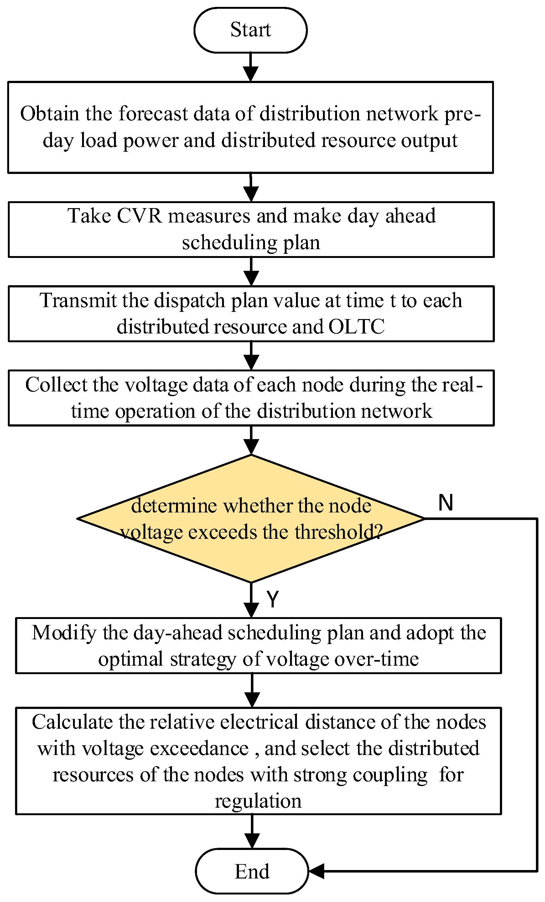
Considering the day-ahead and day–day optimal operation strategy of the distribution network comprehensively, the flexible resource multi-time scale control strategy of the distribution network under the voltage–load regulation architecture proposed in this paper can effectively reduce the system load demand while ensuring the stability of the power network operation. The detailed implementation process is shown in Figure 2, which consists of the following steps:
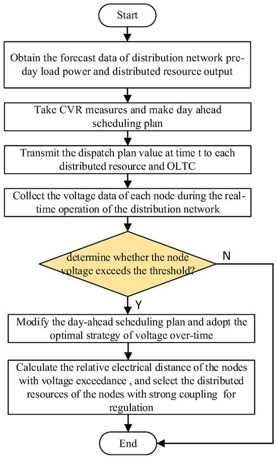
Figure 2.
The process of multi-time scale optimization operation.
Step 1: The forecast data of the load power of the distribution network and the output of distributed resources are obtained.
Step 2: Based on the proposed day-ahead optimal scheduling model, with the minimum daily energy as the optimization goal, the optimal day-ahead scheduling plan for OLTC gear adjustment and distributed resource output is solved to achieve the effect of pressure reduction and energy saving.
Step 3: The dispatch plan value at time t is transmitted to each distributed resource and OLTC.
Step 4: The system periodically monitors nodal voltage measurements at 15 min intervals during real-time grid operation. If no voltage magnitude exceeds the predefined operational thresholds (0.94–1.06 p.u.), the intraday scheduling scheme is deactivated. Conversely, upon the detection of any voltage limit violation, the control protocol immediately initiates Step 5 for corrective action.
Step 5: The day-ahead dispatch schedule is dynamically adjusted by implementing the intraday optimal operation strategy. This coordinated control approach simultaneously optimizes three key objectives: (1) minimizing the total system energy consumption, (2) maximizing flexible resource utilization, and (3) reducing both reactive power adjustments and voltage deviations. The control actions comprise coordinated OLTC tap position adjustments and prioritized dispatch of distributed resources at nodes exhibiting the strongest electrical coupling, as determined by . These corrective measures are executed through fast control commands to ensure voltage stability restoration while maintaining operational continuity until the subsequent day-ahead dispatch cycle is activated.
5. Case Study
5.1. Parameter Settings
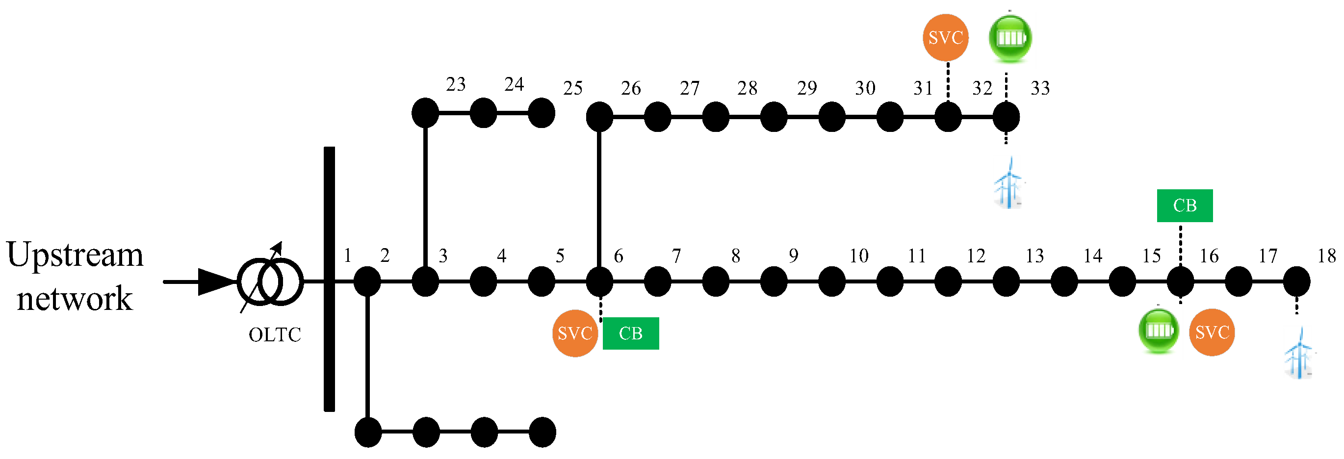
In order to verify the feasibility of the proposed method, the improved IEEE33-node system was used for simulation. The system structure is shown in Figure 3. The reference value of the system voltage was 12.66 kV, the reference value of the power was 1 MVA, and the total and reactive power of the system were 3715 kW and 2300 kVar, respectively. The allowable fluctuation range of node voltage was [0.94, 1.06] p.u., and the maximum allowable maximum current of the branch was 500 A. The OLTC was connected to the branch of Node 1 connected to the superior power grid. There were 12 adjustment gears, the adjustment step was 0.01, the adjustment range was [0.94, 1.06], and the maximum adjustment time was 5. A static VAR compensator (SVC) was connected to Nodes 6, 16, and 32, and the reactive power regulation range was [−100 kVar, 300 kVar] for all. A capacitor bank (CB) was connected to Node 6 and Node 16. The maximum number of operational groups was 10, with each group having 100 kVar, and the maximum switching frequency was 5. The rated capacity of energy storage access nodes 16 and 33 was 2000 kWh, the rated active power values were 300 kW and 200 kW, respectively, the upper and lower limits of capacity were 90% and 20%, and the charge and discharge efficiency rates were 0.9. Fan A-Nodes 18 and 33 each had a capacity of 1000 kW.
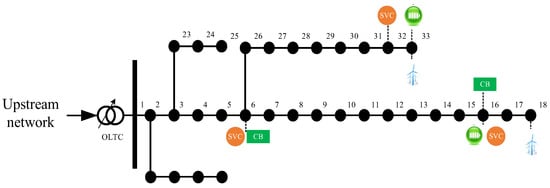
Figure 3.
The topology of the concerned modified network.
5.2. Load Prediction and Error Verification
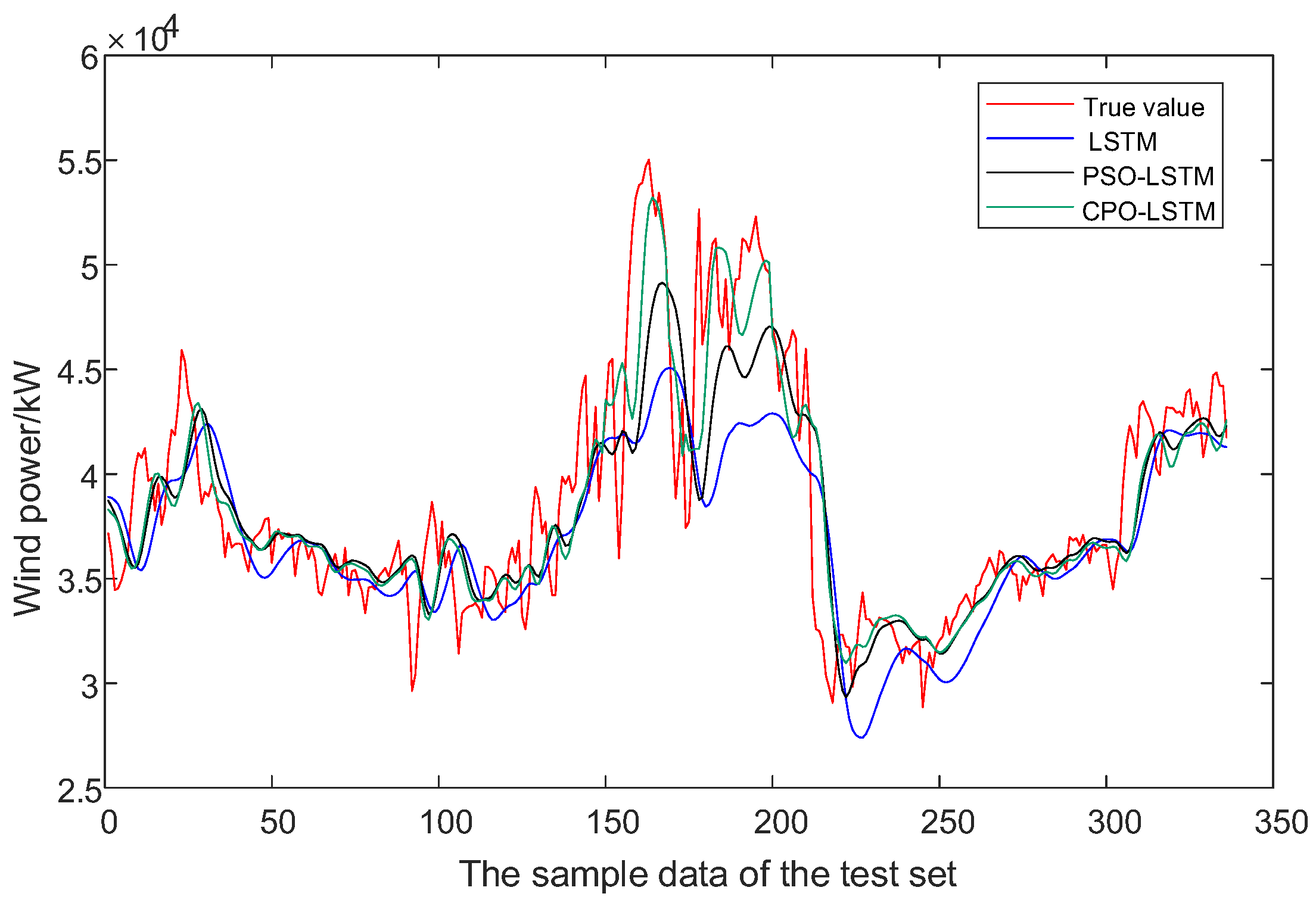
The data used in this paper were derived from the wind load data of a wind farm from 1 July 2022 to 12 July 2022, and they were updated every 15 min, with a total of 1152 groups. The proportion of training and test sets was set to 70% and 30%, respectively, in chronological order, and the data were normalized. For the traditional LSTM prediction model, the wind load data of the first 11 samples were selected to predict the wind load of the last sample. The numbers of input, output, and hidden layer nodes were set to 11, 1, and 20, respectively, and the number of iterations was 1000. The back-propagation algorithm was the Adam algorithm. The tanh function was selected as the activation function. The learning rate was set to 0.005 at the beginning of the training and to 0.0005 after 800 iterations. For a fair comparison, both CPO and PSO optimizers were configured with identical parameter ranges: the range of learning rate lr was set to [0.001, 0.01], the range of network training times was set to [10, 100], the range of hidden layer node number L1 and L2 was set to [1, 200], the population number was 10, and the number of iterations was 1000.
Figure 4 presents a comprehensive comparison of the prediction performance across the different models. While the conventional LSTM captured the general trend of wind power load variations, it showed noticeable deviations during critical operational periods—particularly at daily load peaks, valleys, and rapid fluctuations. The PSO-optimized LSTM demonstrated improved prediction capability compared to the baseline, achieving better alignment with actual measurements. However, the proposed CPO-LSTM exhibited the most accurate tracking performance, maintaining superior consistency with the true load profile throughout the entire observation period. This enhanced performance was especially evident during high-variability conditions, where the CPO optimization effectively reduced both phase delays and amplitude deviations in the predictions, resulting in the most reliable load forecasting results among the three approaches.
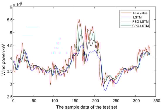
Figure 4.
The wind power prediction effect of each model.
In order to more accurately reflect the performance comparison of the three models, four indexes, namely the RMSE, mean absolute error (MAE), mean absolute percentage error (MAPE), and determination coefficient (R2), were calculated between the predicted load data and the real load data, as shown in Table 1. The analysis demonstrated that the CPO-LSTM model achieved significantly higher prediction accuracy than both the traditional LSTM and PSO-LSTM approaches, exhibiting superior performance across all evaluation metrics. This comprehensive comparison confirmed the effectiveness of the CPO optimization strategy for enhancing wind power forecasting accuracy compared to alternative methods.

Table 1.
Comparison of performance of wind power forecasting model.
5.3. Day-Ahead Optimization Analysis of Distribution Network
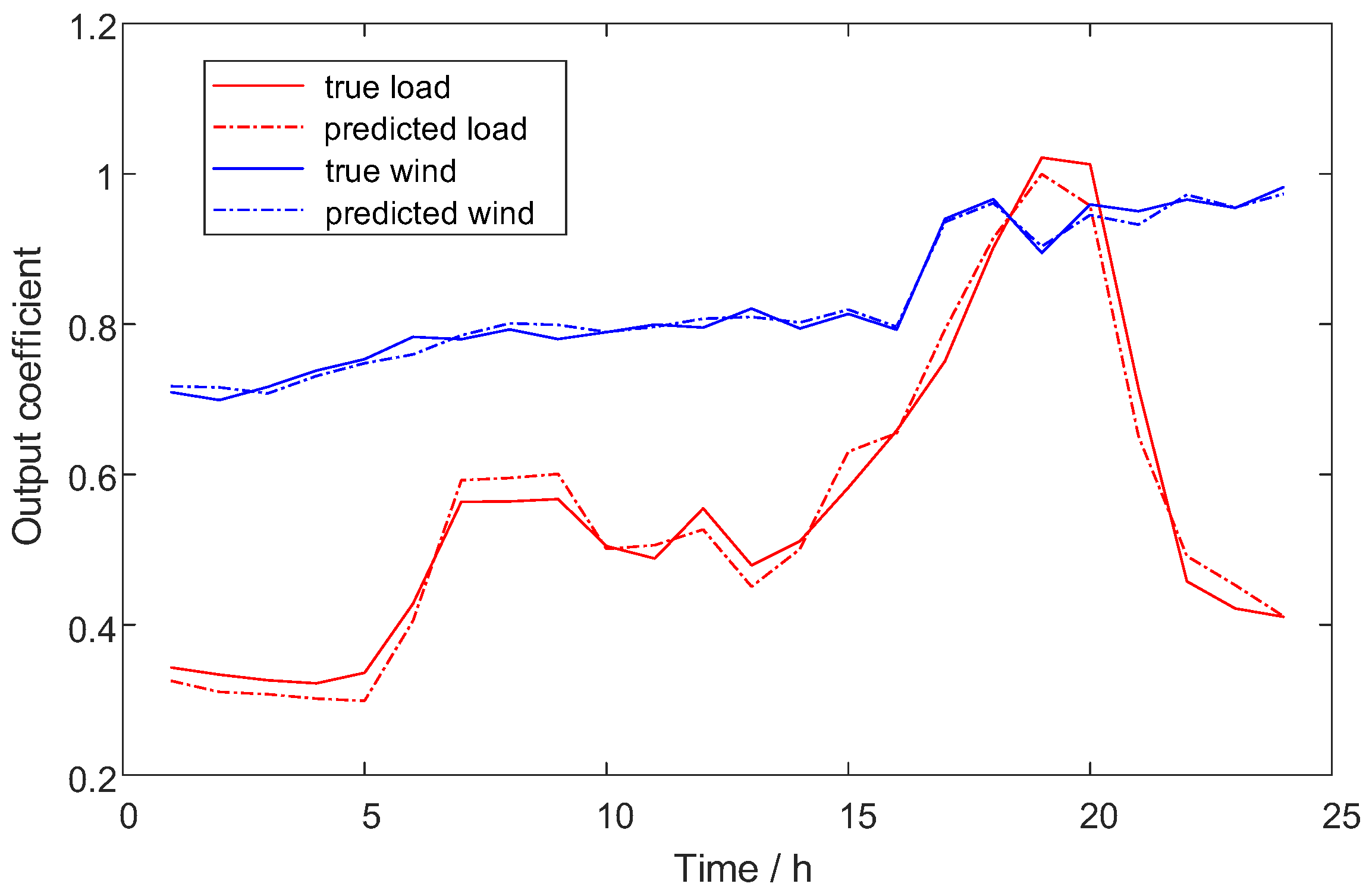
The load forecasting method proposed in this paper was used to train and predict the summer load of a certain area in China. Combined with the prediction results of the above-mentioned test set of wind power, the magnitude was scaled to adapt to the power level of the distribution network. The daily force prediction results of wind power and load are shown in Figure 5. Furthermore, the proposed load forecasting method was specifically calibrated for summer peak conditions in Chinese urban grids, where air conditioning loads dominated (~50% of total demand). Given the prevalence of modern inverter-based AC units with voltage-stabilizing rectifier–capacitor circuits—which exhibit near-constant power characteristics—we adopted a conservative ZIP parameter ratio of 3:2:5 (Z:I:P) for all nodal loads.
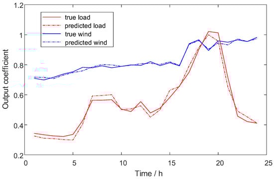
Figure 5.
Load demand and wind power forecast curves.
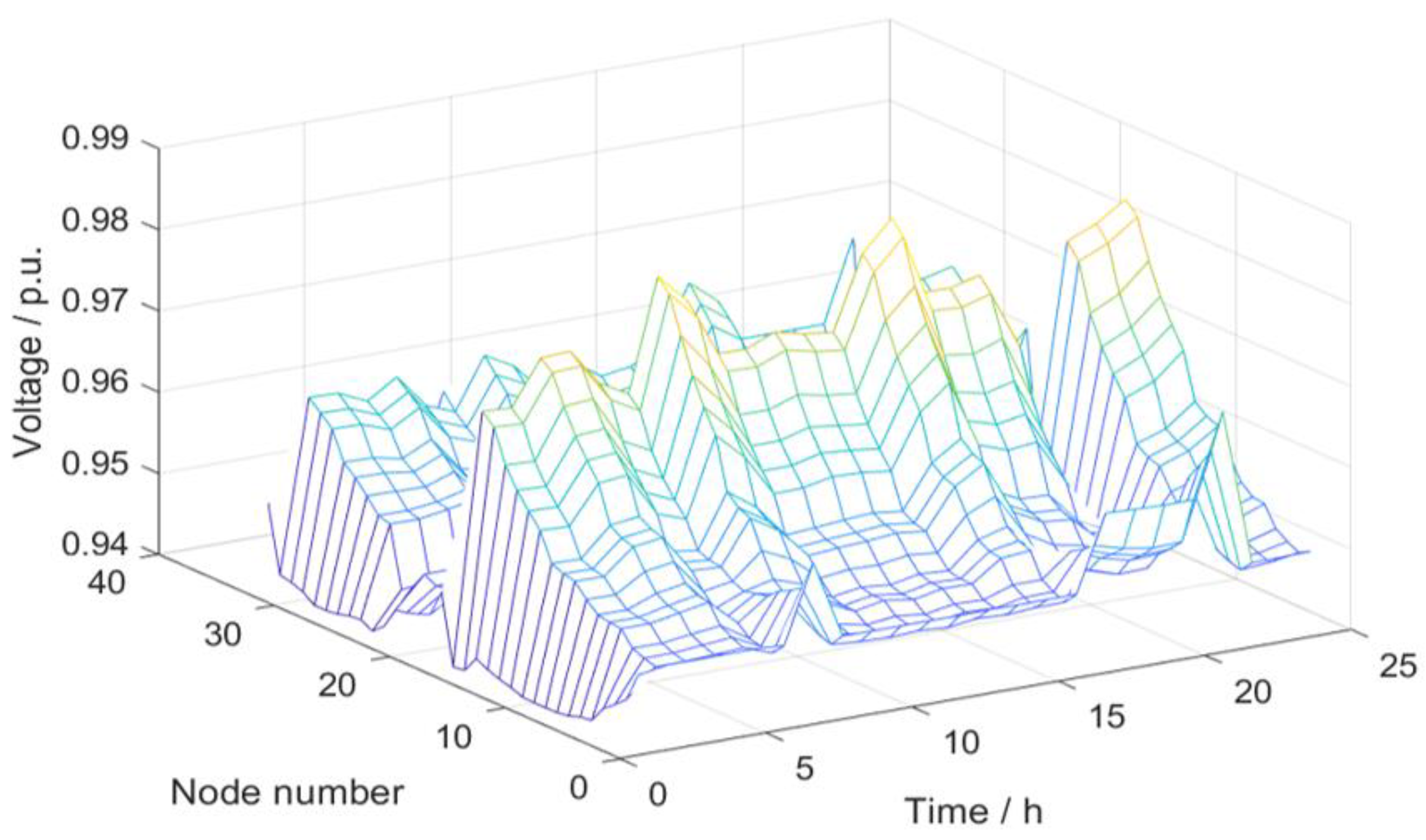
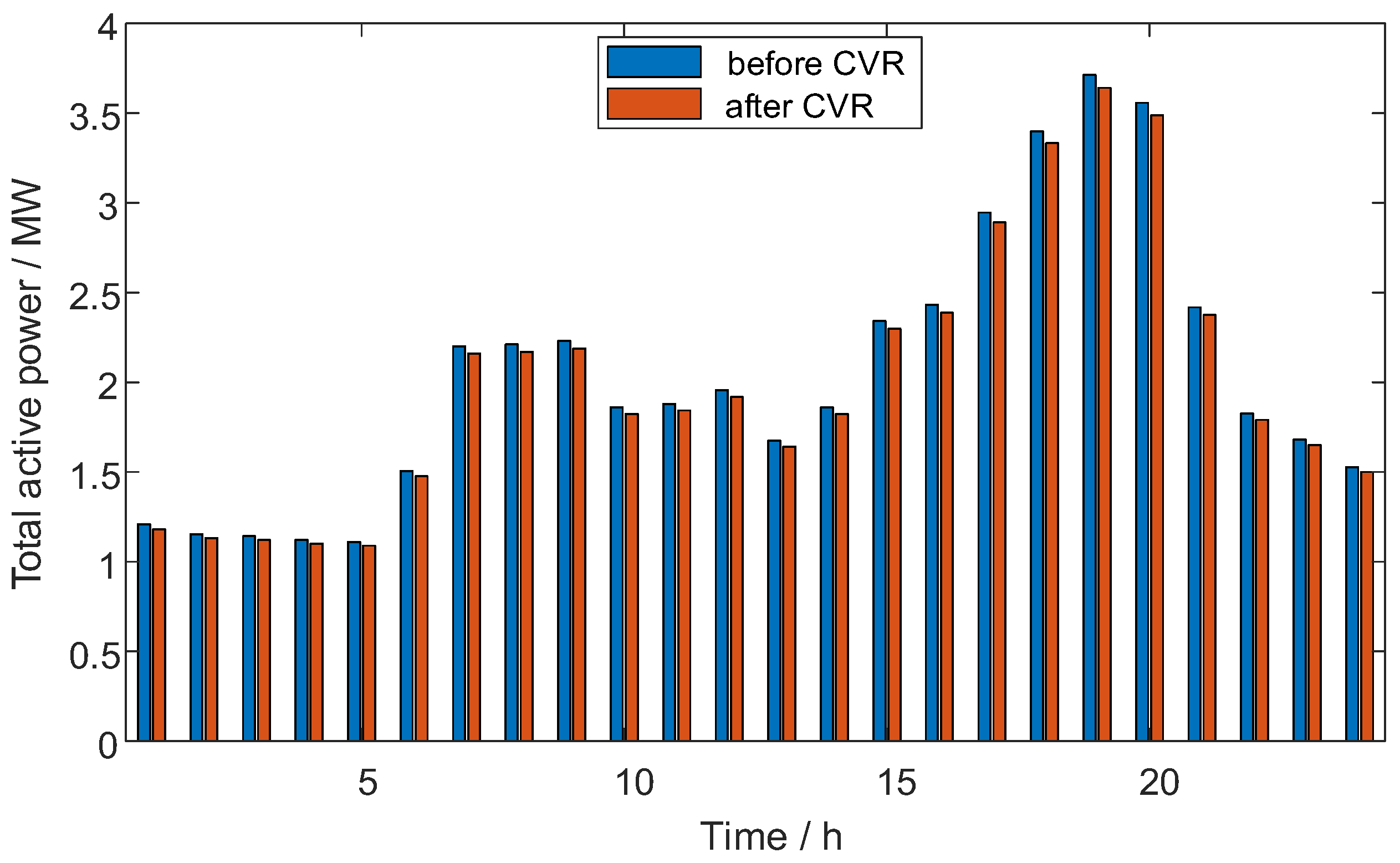
Load prediction results were substituted into the distribution system in Figure 3. Based on the proposed optimization operation strategy for distribution networks, when the voltage margin was sufficient, the optimal OLTC adjustment gear and system voltage were obtained by implementing the CVR strategy, with the minimum daily power consumption of the distribution network as the optimization objective, as shown in Figure 6 and Figure 7, and the total power demand before and after system optimization is shown in Figure 8.
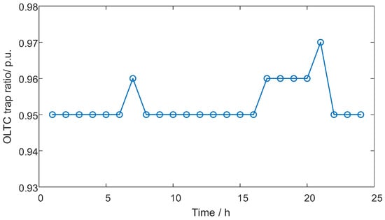
Figure 6.
The OLTC gear’s change diagram.
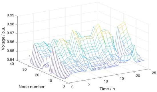
Figure 7.
Node voltage distribution 24 h after CVR optimization.
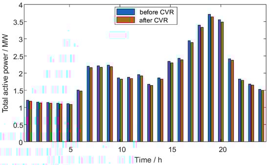
Figure 8.
Changes in the 24 h total power demand of the system before and after CVR optimization.
As demonstrated in Figure 6, the OLTC tap position exhibited dynamic adjustments corresponding to load variations under the CVR strategy. During low-load periods (00:00–06:00), the tap position maintained its value at −5 to ensure voltage adequacy at network terminals. As load progressively increased (07:00–21:00), the tap position increased to −3 to maintain nodal voltage stability while implementing CVR. This coordinated adjustment followed the load profile to minimize system energy consumption without violating voltage constraints. Figure 7 confirms that all nodal voltages remained above 0.94 p.u. post-optimization, fully complying with the power supply voltage standard. The energy-saving effect is quantitatively illustrated in Figure 8. Before optimization, the daily energy consumption of the system was 48.9621 MW·h, and after optimization, the daily energy consumption of the system was 48.0284 MW·h, reducing the daily energy consumption by 1.906%.
5.4. Intraday Optimization Analysis of the Distribution Network
When the deviation between the day-ahead load forecast result and the intraday actual load is relatively small, the intraday dispatching plan correction is not frequent, and the normal and stable operation of the power grid can still be guaranteed. After real-time monitoring, there was a slight difference between the total energy consumption of the day-ahead predicted system and the actual total energy consumption, as shown in Table 2.
Table 2.
Comparison of system energy consumption before and after optimization.
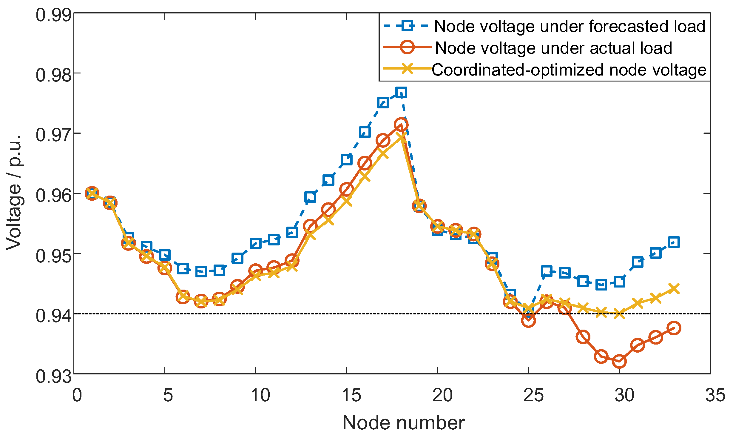
In order to further verify the feasibility of the proposed strategy at the moment when the voltage exceeded the limit, it was assumed that, at 19:00, there was a significant deviation between the predicted value of the pre-day load and the actual value of the intraday load at Nodes 30 and 18, and the output coefficient increased sharply from 0.99 to 1.8, resulting in a surge in the load power demand of nodes, and the system voltage dropped below the safe operating range (see Figure 9). The voltage curve changes from a blue line to an orange line. In this scenario, the proposed method was adopted, the intraday optimization operation strategy was used to respond quickly, the OLTC gear was adjusted, and the distributed resource was selected for regulation according to the electrical distance, so as to realize the rapid voltage recovery and ensure the optimal regulation power of the controlled resource. As shown by the yellow line in Figure 9, in the optimized distribution system, the voltage of all nodes was restored to the specified range.
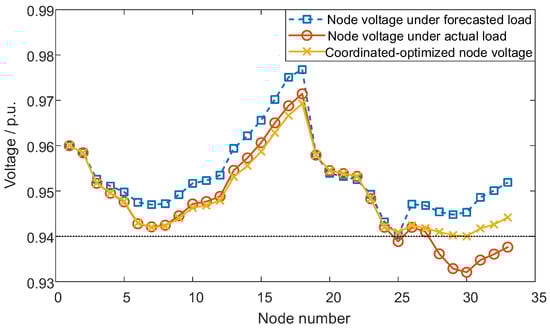
Figure 9.
The voltage of each node in the system at 19:00 before and after optimization.
In the intraday optimal operation strategy, the OLTC remained unchanged from the initial CVR configuration due to minor voltage limit violations. Following the proximity-based regulation principle for distributed resources, the SVC at Node 16 increased its reactive power compensation capacity from 273.3 kVar to 300 kVar, with CB-switching groups increasing from 0 to 3 units. Meanwhile, the reactive power of the SVC at Node 32 was adjusted from 220 kVar to 300 kVar, and the number of CB-switching groups at Node 6 increased from 1 to 5. All other distributed resources maintained their original output levels throughout the optimization process.
At 19:00, the initial power demand of the distribution system was 3.6934 MW. After the day-ahead scheduling strategy was implemented, the total power demand of the system was reduced to 3.6096 MW. Due to the voltage exceeding the limit, the intraday optimization operation strategy was further adopted to raise the voltage at this time, and the system power demand increased to 3.6164 MW. While maintaining the stability of the grid operation, the power demand was still reduced by 1.67%. Therefore, the intraday optimal operation strategy proposed in this paper can not only effectively reduce the total energy consumption of the system and ensure the stability of the operating voltage but also improve the flexibility of intraday scheduling and optimize the overall operating efficiency of the system.
6. Conclusions
To enhance distribution networks’ operational control capabilities and mitigate the impact of load forecasting uncertainties on multi-timescale operations, this paper proposes a CPO-LSTM-based load forecasting method that improves prediction accuracy. Based on the predicted load curve, a multi-time scale control framework of the power distribution network considering CVR technology was further constructed. In the day-ahead scheduling stage, the regulation plan of the OLTC gear and distributed resources was established under the CVR framework to reduce the peak load of the distribution network on the upper power network. In the intraday optimization stage, the real-time adjustment mechanism of OLTC gear was designed for the possible voltage overstep, and the real-time control strategy of flexible adjustable resources based on electrical distance was proposed to realize the rapid voltage recovery of the grid and enhance the stability and robustness of the system. Finally, the IEEE33-node system was used as an example to verify the effectiveness of the proposed strategy.
For practical implementation and further research, three key directions are identified:
- Uncertainty-Aware Optimization: Future work will integrate probabilistic forecasting and interval optimization techniques to address load prediction errors and renewable generation variability, enhancing robustness against real-world uncertainties.
- Market-Integrated Resource Coordination: We plan to develop price-responsive mechanisms incorporating demand-side flexibility, distributed PV-storage hybrids, and two-layer incentive structures to bridge technical optimization with economic signals.
- Field Validation and Implementation: Building on the current simulation-based validation, our subsequent research will focus on field-data-driven refinement of the CVR framework. High-resolution measurements of nodal load compositions (Z/I/P ratios) will be performed using smart meters. The CVR factor (fCVR) will be empirically quantified under real-world operating conditions through controlled voltage reduction trials.
Author Contributions
Investigation, D.J.; resources, D.J.; writing—original draft preparation, Z.R.; supervision, K.L.; project administration, K.H.; writing—review and editing, Z.L. All authors have read and agreed to the published version of the manuscript.
Funding
This work was supported by the project “Smart Grid-National Science and Technology Major Project” [grant number 2024ZD0800804].
Data Availability Statement
Data are contained within the article.
Conflicts of Interest
Author was employed by the company. The remaining authors declare that the research was conducted in the absence of any commercial or financial relationships that could be construed as a potential conflict of interest.
References
- Fan, R.; Sun, R.J.; Liu, Y.T. Load recovery reduction method considering air conditioning demand response. Trans. China Electrotech. Soc. 2022, 37, 2869–2877. [Google Scholar]
- Han, S.; Ruan, S.; Lu, J.; Guo, X.; Mo, Y. Central air conditioning demand response capability evaluation method. In Proceedings of the 2024 4th International Conference on Electronic Materials and Information Engineering (EMIE), Guangzhou, China, 12–14 June 2024; pp. 133–137. [Google Scholar]
- Wang, S.; Li, J.; Chu, T.; Yu, P. Microgrid multi-time scale rolling optimization and modification scheduling considering the decision of air conditioning users. IEEE Access 2025, 13, 49934–49944. [Google Scholar] [CrossRef]
- Chen, X.; Li, K.; Mi, Z.; Wang, F. An air conditioning control method based on non-measurement thermal comfort standard correction for demand response. IEEE Trans. Ind. Appl. 2024, 60, 4736–4748. [Google Scholar] [CrossRef]
- Xu, C.; Inuiguchi, M.; Hayashi, N.; Raymond, W.J.; Mokhlis, H.; Illias, H.A. Enhancing reinforcement learning-based energy management through transfer learning with load and PV forecasting. IEEE Access 2025, 13, 43956–43972. [Google Scholar] [CrossRef]
- Çetinkaya, M.; Acarman, T. Next-Day Electricity Demand Forecasting Using Regression. In Proceedings of the 2021 International Conference on Artificial Intelligence and Smart Systems (ICAIS), Coimbatore, India, 25–27 March 2021; pp. 1549–1554. [Google Scholar]
- Sui, S.; Yu, H.; Jian, Z.; Zhao, Y. Research on electric power large load forecasting and billing based on improved adaptive Kalman filter. Comput. Meas. Control 2023, 31, 149–155. [Google Scholar]
- Li, X.; Li, Z.; Liu, J. A study on medium and long-term load forecasting in a region based on time series analysis. Mod. Ind. Econ. Informatiz. 2024, 14, 282–283+287. [Google Scholar]
- Ye, Y.; Zhang, J. Short-time power load forecasting by SVM based on time series. Mod. Inf. Technol. 2020, 4, 17–19. [Google Scholar]
- Xuan, Y.; Si, W.G.; Zhu, J.; Sun, Z.Q.; Zhao, J.; Xu, M.; Xu, S. Multi-model fusion short-term load forecasting based on random forest feature selection and hybrid neural network. IEEE Access 2021, 9, 69002–69009. [Google Scholar] [CrossRef]
- Chen, X.F.; Chen, W.R.; Dinavahi, V.; Liu, Y.; Feng, J. Short-term load forecasting and associated weather variables prediction using ResNet-LSTM based deep learning. IEEE Access 2023, 11, 5393–5405. [Google Scholar] [CrossRef]
- Han, F.J.; Wang, X.H.; Qiao, J.; Shi, M.J.; Pu, T.J. A review of AI-based load forecasting in new-type power systems. Proc. CSEE 2023, 43, 8569–8592. [Google Scholar]
- Liu, Y.; Bai, X.F.; Chen, S.S.; Gao, J.; Zhao, B.; Hu, C. Summer peak load forecasting model based on bi-level optimization. Electric Power Inf. Commun. Technol. 2025, 23, 11–17. [Google Scholar]
- Zhu, Y.-R.; Wang, J.G.; Sun, Y.Q.; Wu, J.J.; Zhao, G.Q.; Yao, Y.; Liu, J.L.; Chen, H.L. Short-term Load Forecasting of CCHP System Based on PSO-LSTM. In Proceedings of the 2023 IEEE 12th Data Driven Control and Learning Systems Conference (DDCLS), Xiangtan, China, 12–14 May 2023; pp. 639–644. [Google Scholar]
- Wei, T.; Pan, T. Short-term power load forecasting based on improved PSO optimized LSTM network. J. Syst. Simul. 2021, 33, 1866–1874. [Google Scholar]
- Thakur, A.S.; Saxena, D. Conservation Voltage Reduction in Distribution Network: Overview and its Challenges. In Proceedings of the 2022 1st International Conference on Sustainable Technology for Power and Energy Systems (STPES), Srinagar, India, 4–8 July 2022; pp. 1–5. [Google Scholar]
- Li, Y.; Duan, R.; Shi, F.; Lv, W.; Li, R. Research on Carbon Reduction Potential of CVR Technology. In Proceedings of the 2024 9th Asia Conference on Power and Electrical Engineering (ACPEE), Shanghai, China, 11–13 April 2024; pp. 885–889. [Google Scholar]
- Preiss, R.F.; Warnock, V.J. Impact of Voltage Reduction on Energy and Demand. IEEE Trans. Power Appar. Syst. 1978, PAS-97, 1665–1671. [Google Scholar] [CrossRef]
- Williams, B.R. Distribution capacitor automation provides integrated control of customer voltage levels and distribution reactive power flow. In Proceedings of Power Industry Computer Applications Conference, Salt Lake City, UT, USA, 7–12 May 1995; pp. 215–220. [Google Scholar]
- Lauria, D.M. Conservation Voltage Reduction (CVR) at Northeast Utilities. IEEE Trans. Power Deliv. 1987, 2, 1186–1191. [Google Scholar] [CrossRef]
- Schneider, K.P.; Fuller, J.C.; Tuffner, F.K.; Singh, R. Evaluation of Conservation Voltage Reduction (CVR) on a National Level; Pacific Northwest National Laboratory (PNNL): Richland, WA, USA, 2010.
- Jha, R.; Fan, W.; Pabst, P.; Guo, Y.; Chun, H. Enhancing Conservation Voltage Reduction with Grid Edge Volt-VAr Control. In Proceedings of the 2023 IEEE PES Grid Edge Technologies Conference & Exposition (Grid Edge), San Diego, CA, USA, 10–13 April 2023; pp. 1–5. [Google Scholar]
- Sun, X.; Qiu, J.; Tao, Y.; Ma, Y.; Zhao, J. A Multi-Mode Data-Driven Volt/Var Control Strategy With Conservation Voltage Reduction in Active Distribution Networks. IEEE Trans. Sustain. Energy 2022, 13, 1073–1085. [Google Scholar] [CrossRef]
- Prajapati, C.P.; Chanana, S. Volt/VAR optimization and control of smart-grid enabled distribution system using CVR. In Proceedings of the 2022 International Conference on Futuristic Technologies, Belgaum, India, 25–27 November 2022; pp. 1–5. [Google Scholar]
- Singh, S.; Pamshetti, V.B.; Singh, S.P. Time Horizon-Based Model Predictive Volt/VAR Optimization for Smart Grid Enabled CVR in the Presence of Electric Vehicle Charging Loads. IEEE Trans. Ind. Appl. 2019, 55, 5502–5513. [Google Scholar] [CrossRef]
- Lakra, N.S.; Bag, B. Reduction in Power Consumption via Integration of CVR with Network Reconfiguration and VAr Control. In Proceedings of the 2021 IEEE 2nd International Conference On Electrical Power and Energy System, Bhopal, India, 10–11 December 2021; pp. 1–5. [Google Scholar]
- Sahu, R.K.; Bag, B.; Lakra, N.S. Maximizing Techno-Economic Benefits Using Combined Approach of CVR, DG and D-STATCOM Placement. In Proceedings of the 2022 IEEE Silchar Subsection Conference Silchar, Silchar, India, 4–6 November 2022; pp. 1–6. [Google Scholar]
- Lu, Z.T.; Wei, Y.H.; Zhou, L.; Peng, Y.B.; Liu, Y.; Shi, W.T.; Chen, G.Q. Voltage reduction and energy saving method for active distribution networks considering distributed generation integration. Electr. Eng. Technol. 2024, (8), 117–120. [Google Scholar]
- Lan, Z.; Yi, B.; Guo, Q.; Li, J.H.; Yang, C.Z. Multi-timescale coordinated control strategy for active and passive resources in medium-low voltage distribution networks. Power Syst. Clean Energy 2025, 41, 10–17+26. [Google Scholar]
- Zhang, Y.L.; Wang, Z.M.; Xue, C.; Qiu, J.Y.; Li, X.T.; Zhou, Q. Two-stage active-reactive power coordinated loss reduction method for distribution networks considering renewable energy integration. Power Syst. Clean Energy 2023, 39, 121–129. [Google Scholar]
- Rahman, M.T.; Hasan, K.N.; Sokolowski, P. Assessment of Conservation Voltage Reduction Capabilities Using Load Modelling in Renewable-Rich Power Systems. IEEE Trans. Power Syst. 2021, 36, 3751–3761. [Google Scholar] [CrossRef]


Disclaimer/Publisher’s Note: The statements, opinions and data contained in all publications are solely those of the individual author(s) and contributor(s) and not of MDPI and/or the editor(s). MDPI and/or the editor(s) disclaim responsibility for any injury to people or property resulting from any ideas, methods, instructions or products referred to in the content. |
© 2025 by the authors. Licensee MDPI, Basel, Switzerland. This article is an open access article distributed under the terms and conditions of the Creative Commons Attribution (CC BY) license (https://creativecommons.org/licenses/by/4.0/).