A Day-Ahead PV Power Forecasting Method Based on Irradiance Correction and Weather Mode Reliability Decision

Abstract

Accurate day-ahead photovoltaics (PV) power forecasting results are significant for power grid operation. According to different weather modes, the existing research has established a classification forecast framework to improve the accuracy of day-ahead forecasts. However, the existing framework still has the following two problems: (1) weather mode prediction and power forecasting are highly dependent on the accuracy of numerical weather prediction (NWP), but the existing classification forecasting framework ignores the impact from NWP errors; (2) the validity of the classification forecasting framework comes from the accurate prediction of weather modes, but the existing framework lacks the analysis and decision-making mechanism of the reliability of weather mode prediction results, which will lead to a significant decline in the overall accuracy when weather modes are wrongly predicted. Therefore, this paper proposes a day-ahead PV power forecasting method based on irradiance correction and weather mode reliability decision. Firstly, based on the measured irradiance, K-means clustering method is used to obtain the daily actual weather mode labels; secondly, considering the coupling relationship of meteorological elements, the graph convolutional network (GCN) model is used to correct the predicted irradiance by using multiple meteorological elements of NWP data; thirdly, the weather mode label is converted into one-heat code, and a weather mode reliability prediction model based on a convolutional neural network (CNN) is constructed, and then the prediction strategy of the day to be forecasted is decided; finally, based on the weather mode reliability prediction results, transformer model are established for unreliable weather and credible weather respectively. The simulation results of the ablation experiments show that classification prediction is an effective strategy to improve the forecasting accuracy of day-ahead PV output, which can be further improved by adding irradiance correction and weather mode reliability prediction modules.

1. Introduction

Under the dual background of the continuous growth of global power and energy demand and the response to global climate change, clean and renewable energy has become an important direction of energy transition. Countries around the world have formulated policies to accelerate the transformation of energy structure, and the year-on-year increase in the global installed capacity of photovoltaic (PV) is a direct manifestation of this behavior [1]. Photovoltaic power generation performance is affected by many factors, including but not limited to meteorological conditions, PV module performance, and so on. Among them, the influence of meteorological elements on PV power is more intuitive and complex, and the coupling relationship between meteorological elements brings randomness, indirectness, and volatility to PV power generation [2]. Therefore, in a new type of power system with high PV power penetration, the characteristics of PV power generation bring new challenges to the safe and stable operation of the power grid and the dynamic balance of power and electricity and become a problem that needs to be solved for the continued development of PV power generation.

To facilitate the further development and application of solar power, a variety of techniques have been proposed and proved to be effective, including flow optimization, microgrid technology, demand response, energy storage configuration, and solar power forecasting [3]. Among them, accurate PV power forecasting can provide prospective support for optimal scheduling decisions and stable, robust power system operation by grid dispatchers [4]. Meanwhile, for power generators, improving forecast accuracy can help PV power plants to reduce economic losses due to power-load mismatch, improve PV operation and management efficiency, and also play an important role for PV power plants to participate in power market transactions. According to different time scales, PV power forecasts are classified into medium- and long-term forecasts, short-term forecasts, and ultra-short-term forecasts. Day-ahead forecasts are categorized as short-term forecasts and are used to forecast solar power generation for the next day one day in advance. Existing day-ahead PV power forecasting methods are classified into physical and data-driven approaches based on modeling principles. Physical methods use numerical weather forecasts, sky images, or satellite imaging to obtain predictions of solar irradiance received by the PV plant and determine the PV power by modeling the photovoltaic conversion of the PV panels and calculating the inverter efficiency [5]. Although physical models have the advantage of better interpretability of physical phenomena and principles, physical modeling requires detailed parameter settings for a specific PV plant and location, while physical forecast models require more mathematical knowledge to be solved, as they are based on mathematical equations describing the PV conversion. The algorithms used involve the solution of complex differential equations [6]. Therefore, the number of studies related to physical forecast models is low.

Data-driven modelling is currently the mainstream method for PV power forecast in the past few days, which uses high-dimensional nonlinear mapping relationships to forecast the PV power in the future time by learning the key information patterns from historical meteorological data, historical NWP data, and historical power data [2]. Many machine learning methods such as support vector machines (SVMs), autoregressive differential moving average model (ARIMA), and artificial neural networks (ANNs) [7] have been applied to build data-driven forecast models with good results. Li et al. [8] used meteorological factors such as temperature, humidity, and sunshine duration to fit a generalized ARMAX model, called ARMAX, a generalized ARIMA forecasting model. Giorgi et al. [9] combined three multistep-ahead forecasting strategies to compare, respectively, the least squares support vector machine (LS-SVM), a neural network known as group method of data handling (GMDH), and a hybrid algorithmic group least squares support vector machine (GLSSVM) for the forecast accuracy of the three models. Tao et al. [10] proposed a short-term forecast model based on the transformer architecture by considering the PV physical modelling data, integrating the site-specific and future time information by setting the physical modelling intermediate variables, and extracting the temporal dependence and feature-to-feature dependence of the two types of data with PV power generation using the parallel architecture, respectively.

Although the data-driven model can learn the daily cycle characteristics of PV power generation from the open dataset, and machine learning can predict PV power generation methods that are direct, deterministic, and relatively accurate [11], it cannot fully learn the close relationship between PV output and weather mode, i.e., PV power generation in different weather conditions exhibits significantly different time-series characteristics specific to each [12]. Then, classification forecast methods were proposed to solve this problem. Classification prediction methods divide the dataset into different weather modes according to the characteristics of meteorological elements, then train the power forecast model under each weather mode separately, and finally select the corresponding power forecast model to execute the forecast according to the weather mode of the time period to be forecasted [13]. Yu et al. [14] constructed a double similar day screening model based on grey correlation analysis and adaptive K-means, which The weather was classified into three types: sunny, cloudy, and rainy, and the combined forecast model based on the deep learning method and kernel density estimation was used to obtain the point forecast results and the intervals of the point forecast errors under different weather modes, respectively. Fang et al. [15] used some statistical indexes, namely, the mean, the standard deviation, the kurtosis, and the skewness, as the characteristics of the historical PV output, and the FCM clustering algorithm was used to classify the historical data into sunny, cloudy, rainy and extreme weather, and then construct a joint forecast model based on XGBoost-GRU for the four weather modes to forecast the PV output power. Wang et al. [16] first reclassified 33 meteorological weather modes in the meteorological standard into 10 weather modes and used a generative adversarial network to achieve the problem of insufficient training datasets for different weather modes. The solar irradiance dataset is expanded, and the enhanced dataset is used to train a weather classification forecast model based on a convolutional neural network to achieve accurate classification of weather modes. Huang et al. [17] In order to reduce the impact of weather on the accuracy of short-term PV power generation forecasts, the weather is classified into sunny, cloudy, and rainy by using the support vector machine (SVM), and the back propagation (BP) neural network based on the optimization of particle swarm optimization (PSO) is constructed.

Overall, the data-driven PV power forecast method based on classification forecast consists of two steps: the first step is to determine or predict the weather mode, and then model training and power forecast are performed based on the weather mode results. The above researchers applied the classification forecast approach in their simulation conditions, which effectively improved the PV power forecast accuracy compared to the forecast without considering different weather modes. However, it is worth noting that the existing PV power classification prediction methods still have the following two problems:

(1)

Both weather mode judgment and PV power model training and forecasting are highly dependent on the accuracy of the NWP. The NWP data serve as the input data for both weather mode judgement and power forecast models, and machine learning algorithms are used in both steps. A lower input accuracy will result in the machine learning method not being able to map the correct results using the learnt patterns, and thus a weather mode judgement correctness decreases and the forecast accuracy of the power forecast model decreases. Existing methods ignore the effect of NWP errors on weather mode and power forecast accuracy.

(2)

Lack of corrective mechanisms for power forecast in the event of weather mode prediction errors. The NWP itself is a source of weather mode prediction errors. When weather mode prediction errors inevitably occur, they lead to the selection of mismatched power prediction models, which in turn result in the degradation of power forecast accuracy. Therefore, corresponding corrective measures are needed to reduce the negative impact of weather mode prediction errors.

To address the above issues, this study proposes a short-term PV power forecasting method based on forecast solar irradiance correction and weather mode reliability prediction. The main contributions are summarized as follows:

(1)

An NWP irradiance correction model based on characterization of coupled properties of meteorological elements and a graph convolutional neural network is proposed. The coupling relationship of meteorological elements is considered to correct the forecast irradiance using NWP data so that the forecast irradiance is closer to the measured irradiance. The data quality of NWP, especially the irradiance data, is improved by mining the influence of each forecast meteorological factor in NWP on the forecast irradiance, which enables the constructed model to correctly learn the nonlinear mapping relationship between irradiance and weather mode and PV output and to improve the weather mode prediction and power forecast accuracy.

(2)

A convolutional neural network-based weather mode reliability prediction model is proposed, and a weather mode prediction result reliability judgment mechanism is designed for the classification forecasting framework. Considering the reliability of the prediction results, a conservative strategy of adopting a unified forecasting model is taken for potentially erroneous weather mode prediction results so that the decision-making of the power forecast model can avoid the negative impacts caused by erroneous weather mode prediction results to the greatest extent possible, and the accuracy of the PV output forecast can be further improved.

The remainder of the paper is organized as follows. Section 2 focuses on the research methodology and technical details of this paper. Section 3 applies the methodology of this study to a real case and compares it with different methods to validate the effectiveness of the proposed methodology. Section 4 concludes and looks forward to this study.

2. Materials and Methods

The proposed research framework is shown in Figure 1, and the work of each step can be summarized as follows:

Step 1: Weather mode clustering. According to the measured irradiance data of the target station, K-means clustering is carried out, and the obtained results are used to classify the weather modes.

Step 2: Numerical weather forecast correction. Using other forecast meteorological elements and forecast irradiance of the target station as input features and the revised irradiance as output, the graph convolutional network (GCN) was constructed to correct the forecast irradiance so that the revised forecast irradiance was closer to the measured irradiance.

Step 3: Weather mode reliability prediction. First, the historical weather mode label obtained by the weather mode cluster is converted into a one-hot code representing the probability of the weather mode occurrence. Secondly, the meteorological features of historical NWP are extracted every day, and then the historical weather mode-thermal coding is used to train the convolutional neural network (CNN)-based weather mode reliability prediction model. Subsequently, when updating the NWP of the day to be predicted, the reliability of the different weather modes is obtained by inputting NWP data into weather mode prediction models. Finally, the maximum reliability value of the weather mode is compared with the reliability threshold. If the former is greater than the latter, the weather mode corresponding to the maximum value is judged as the trusted prediction result. Otherwise, the prediction results of the weather mode will be regarded as untrusted.

Step 4: Classification training of PV power forecasting model. First, the overall transformer model is trained with historical data for the complete training set and applied to scenarios where the weather mode prediction results are not reliable. Secondly, the training set is divided into several subsets according to the weather mode label, and the transformer models specialized for classification forecast are trained using the data of each subset.

Step 5: PV power classification forecast. When the maximum reliability of the weather mode forecast results is higher than the reliability threshold, the classification forecast strategy is adopted; on the other hand, the overall transformer model is used to forecast the PV power generation on the same day to avoid the forecast accuracy decline caused by the wrong judgment of the weather mode and the wrong invocation of the forecasting model.

2.1. Weather Mode Clustering

Irradiance is an important meteorological feature of PV power forecast, and it is also one of the indicators to distinguish different weather modes. Therefore, the weather mode results are obtained by clustering the target stations according to the measured irradiance. In order to better classify different weather modes according to the overall characteristics of the daily irradiance curve, the common K-means clustering method is chosen. K-means clustering is a common distance-based clustering algorithm that aims to divide a dataset into K clusters [18]. The goal of the algorithm is to minimize the sum of distances from sample points in the cluster to the cluster center, as shown in Formula (1) [18]:

$$J={\displaystyle \sum _{i=1}^K{\displaystyle \sum _{x\in C_i}{‖x-{\mu }_i‖}^2}}$$

(1)

By repeatedly adjusting the location of the cluster center, K-means continuously optimizes the tightness within the clusters, thereby obtaining clusters that are as compact and separate from each other as possible. K-means usually uses Euclidean distance to measure the distance between the sample point and the cluster center, and its formula is as follows [18]:

$$d(x,\mu )=\sqrt{{\displaystyle \sum _{j=1}^n{(x_j-{\mu }_j)}^2}}$$

(2)

For the measured irradiance, the irradiance curve of 96 points every 15 min a day is converted into a 96-dimensional vector, and the difference in the shape of the irradiance curve is converted into the Euclidean distance between the sample points, which can obtain a better classification effect. At the same time, through clustering, we can identify the outliers or noises in the original data and improve the data quality.

2.2. Numerical Weather Forecast Correction

The meteorological elements most directly related to PV output are irradiance, and other meteorological elements such as wind speed, wind direction, humidity, temperature, and cloud cover do not have a direct impact on photovoltaic output (showing a weak correlation with PV output), and the irradiance data and photovoltaic power almost show a completely consistent trend of fluctuation. It is of great significance to improve the accuracy of solar power prediction by improving the accuracy of irradiance numerical prediction. Considering that there is a certain error between the forecast irradiance of numerical weather forecast and the measured irradiance, it is necessary to correct the forecast irradiance of the target PV power station to improve the prediction accuracy.

In graph neural networks, the graph is composed of a series of nodes and edges between nodes, and both nodes and edges can contain rich data information. Therefore, the graph structure is extremely suitable for describing the association relationship between various entities, such as social [19], traffic [20], communication [21], power [22], and other networks. Each forecast meteorological element of the target station and its relationship can be represented by a graph structure; each forecast meteorological element can be regarded as a graph node, and the correlation between each meteorological element can form the edge of the graph. Therefore, GNN uses a neural network to learn the graph structure data and extract the features and patterns in the graph structure data, which can well meet the requirements of the graph learning task. The deep learning algorithm under this framework can directly learn the graph structure data. By defining certain rules for nodes and edges in the graph structure, the graph structure data can be converted into a standardized representation, and different neural networks can be selected according to actual needs for training and learning [23]. It has excellent performance in the tasks of node classification, node prediction, edge prediction, edge information propagation, and graph clustering. The classification of graph neural networks mainly includes graph attention networks, graph automatic encoders, and graph convolutional neural networks.

In this study, the graph convolutional network model is used to modify the forecast irradiance. Graph convolutional network (GCN) is a kind of deep learning model that deals with graph structure data. By aggregating the feature information of nodes themselves and their neighbors, the node representation is updated to capture the local and global structure features of graph data [24]. The structure of the GCN model is shown in Figure 2, and the core idea is to extend traditional convolution operations from Euclidean spaces (such as images and grids) to non-Euclidean spaces. GCN performs convolution operations on the graph structure in the spectral domain, and the graph structure in the spectral domain is defined as follows [24]:

$$g_{\theta }★x=U{g}_{\theta }{U}^{T}x$$

(3)

where g_θ is the convolution kernel, ★ represents the graph convolution operator, x represents the scalar information of each node on the graph, and U is the eigenvector matrix of the normalized graph Laplacian matrix.

The calculation of GCN is an iterative process in which adjacent nodes and their own information are constantly considered. Each iteration is a feature recombination. The features of the next layer are the graph convolution of the features of the previous layer, and the graph convolution expression is as follows [24]:

$$H^{l+1}={\tilde{D}}^{-{\displaystyle \frac{1}{2}}}\tilde{A}{D}^{-{\displaystyle \frac{1}{2}}}{H}^l{W}^l$$

(4)

where $H^{l+1}$, $H^l$ represents the node eigenmatrix, $\tilde{A}$ represents the adjacency matrix with $\tilde{A}$ self-ring added (the addition of the adjacency matrix and the identity matrix), $\tilde{D}$ is the degree matrix corresponding to $\tilde{A}$, and $W^l$ is the learnable weight matrix of the l layer. Input the original data $X$ and the adjacency matrix $A$ that characterizes the structure characteristics of the graph, and the model output is $Z=f(X,A)$.

2.3. Weather Mode Reliability Prediction

Based on the results of the weather mode clustering, we classify the weather into different categories so we can train the corresponding PV power prediction model using historical NWP data for different weather modes. These prediction models perform better with the corresponding weather characteristics than unified prediction models trained with all historical data. When performing the forecasting step, we need to first make a prediction of the future weather mode through the NWP data and select the appropriate forecasting model through the forecast results. However, the accuracy of NWP data directly affects the accuracy of weather mode prediction results. If the wrong judgment of the weather mode leads to the selection of the wrong prediction model, the accuracy of prediction results will be greatly reduced. Currently, the reliability of the weather mode prediction results, which is the probability that the weather mode prediction is correct, is particularly important.

Therefore, the problem is transformed into an accurate prediction of the results of the classification of future weather modes, which is a special classification task. Convolutional neural networks (CNNs) have achieved remarkable results in classification prediction tasks, and their core advantage lies in their efficient feature extraction and modeling ability for multi-modal data such as images, texts, and time series. Through local perception, parameter sharing, and hierarchical feature extraction, CNNs achieve high efficiency, robustness, and precision in classification tasks. Therefore, this study chooses CNN to achieve weather mode reliability prediction [25].

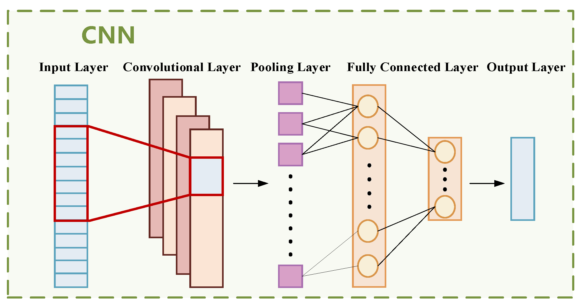
The CNN model structure, as shown in Figure 3, includes input layer, convolutional layer, pooling layer, fully connected layer, and output layer [26]. The convolution kernel (filter) slides on the input, calculates the dot product sum of the local region, and obtains the output feature map [25]:

$$Z_{i,j}={\displaystyle \sum _{m=0}^{f-1}{\displaystyle \sum _{n=0}^{f-1}{x}_{i+m,j+n}\cdot w_{m,n}+b}}$$

(5)

where $Z_{i,j}$ is the element in the output feature map, $x_{i+m,j+n}$ is the element in the input feature map, $w_{m,n}$ represents the weight in the convolution kernel (filter), and $b$ is the biased term, which is a constant. Like weather mode clustering, weather mode reliability prediction takes the irradiance modified in the second step as input, so the dimension of the input feature is 1, and a 1-dimensional convolution operation is applied.

The pooling layer reduces computational complexity by reducing the size of the feature map. This is done by selecting the maximum or average value within the pooled window. This helps to extract the most important features. The pooling layer is done using the most common max pooling method.

The output of the convolutional neural network is the probability judged for each weather mode, for which it is necessary to code the historical weather mode classification results before making weather mode reliability predictions. The principle of coding is to obtain the coding of $i$ positions according to the clustering result $i$. If it belongs to this category, the value of this position is 1, and the value of other positions is 0. Through 01 coding, the probability of the corresponding weather mode is set to 100% in the historical data, and the non-corresponding weather mode is set to 0%. Subsequently, the output result of the reliability prediction of the test set is the probability that this day belongs to each weather mode, in other words, the reliability of the weather mode of this day is obtained.

2.4. Photovoltaic Power Classification Forecast

According to the weather mode classification of the training set and the reliability prediction of the test set, we can use the data classification under different weather modes of the training set to train the corresponding model under each category and the unified model trained with all the data. When forecasting the test set, according to the result of the weather mode reliability prediction, if the probability of the weather mode is greater than the set threshold, the weather mode prediction of this day is credible, and the corresponding weather mode prediction model is used to forecast this day. If the probability does not meet the conditions, the unified forecasting model is used to forecast the day.

As a time-series forecasting problem, the conventional RNN model has the problem of gradient explosion. The self-attention mechanism can capture the dependence between any two positions in the sequence and solve the gradient disappearance problem of RNN. Therefore, in this study, we choose the transformer model for day-ahead PV power forecasting.

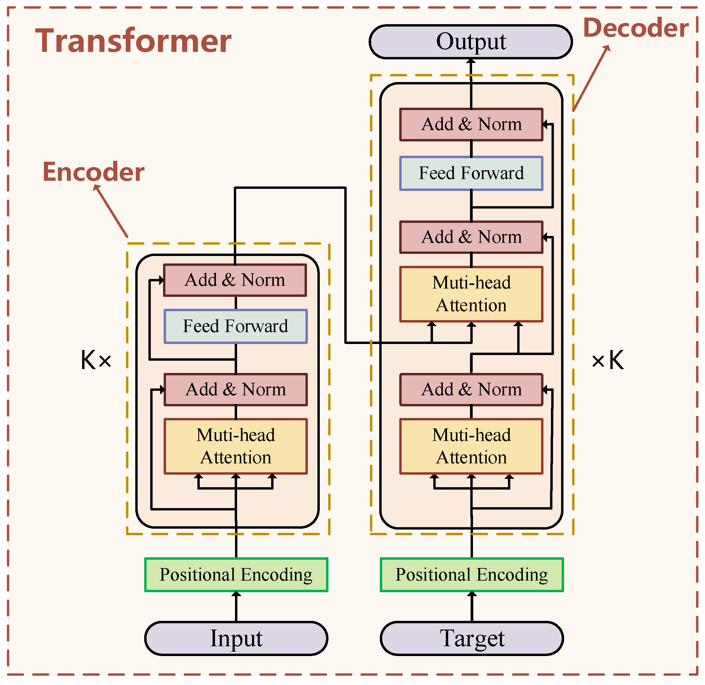
Transformer is a deep learning model based on an attention mechanism, mainly used to solve sequence-to-sequence problems. Compared to RNNS or LSTMS, transformer can deal with long-distance dependence problems more efficiently and can parallelize training [27]. As shown in Figure 4, the transformer model is mainly composed of an encoder and a decoder. Both parts consist of multiple identical layers stacked together, each of which in turn consists of two sub-layers: multi-head self-attention mechanisms and location-feedforward neural networks. There is a residual link around each sublayer, and the output is processed by layer normalization. Because transformer does not use the structure of RNN but uses global information, transformer introduces positional encoding and uses sine (cosine) functions to generate position vectors and add them with input feature embeddings. The purpose is to preserve the relative or absolute position of the input feature in the sequence. The location coding formula is as follows [27]:

$$\begin{array}{l}P{E}_{(pos,2i)}=\sin ({\displaystyle \frac{pos}{{10000}^{\frac{2i}{d}}}})\\ P{E}_{(pos,2i+1)}=\cos ({\displaystyle \frac{pos}{{10000}^{\frac{2i}{d}}}})\end{array}$$

(6)

where $pos$ represents the position of the input feature in the time series, $d$ represents the dimension of PE, $2i$ represents the dimension of even numbers, and $2i+1$ represents the dimension of odd numbers (i.e., $2i\le d$, $2i+1\le d$).

At the heart of the transformer model is the self-attention mechanism, which allows the model to process each element while focusing on information elsewhere in the sequence. By calculating the dot product between query, key, and value, the correlation weight of each input feature with the other input features is obtained. The input feature embedding generates Q, K, and V matrices through linear transformation and calculates the attention weight [27]:

$$Attention(Q,K,V)=\mathrm{softmax}({\displaystyle \frac{Q{K}^T}{\sqrt{d_k}}})\mathrm{V}$$

(7)

where $dk$ is the dimension of the key vector, the scaling factor $\sqrt{d_k}$ is used to prevent the dot product value from being too large and causing the gradient to disappear.

To capture richer features, transformer uses a multi-head attention mechanism. It divides Q, K, and V into multiple subspaces, each of which computes attention independently, and finally concatenates the results. This mechanism allows the model to focus on different parts of the sequence [27]:

$$MultiHead(Q,K,V)=Concat(hea{d}_1,\dots ,hea{d}_h)W^O$$

(8)

Each head is calculated as:

$$hea{d}_i=Attention(Q{W}_i^Q,K{W}_i^K,V{W}_i^V)$$

(9)

3. Simulation and Discussion

3.1. Dataset Description

The simulation data used in this study are derived from the power generation data of a centralized PV power plant in the Inner Mongolia Autonomous Region, China, which has a total installed capacity of 75 MW. The date range of the data is from 1 January 2023 to 31 December 2024, with a temporal resolution of 15 min. The dataset consists of actual PV power and measured and predicted NWP values of seven meteorological factors (irradiance, cloudiness, temperature, humidity, wind speed, wind direction, and barometric pressure) with finite power labels for each time point. The dataset is divided into a training and a test set, where about 75% of the data is used to train the model and the remaining 25% of the data is used to test the effectiveness of the proposed method. Thus, 1 January 2023 to 31 May 2024 is classified as the training set and 1 June 2024 to 31 December 2024 is classified as the test set. After removing the data with outliers and missing values, 594 days of full run data remain. The case studies were implemented using the deep learning Python library PyTorch1.12.0 + cuda11.3. All experiments were performed on a laptop with an Intel Core i5-1135G7 (2.50 GHz) CPU, NVIDIA MX 450 GPU, and 16 GB RAM.

3.2. Results of Weather Mode Clustering

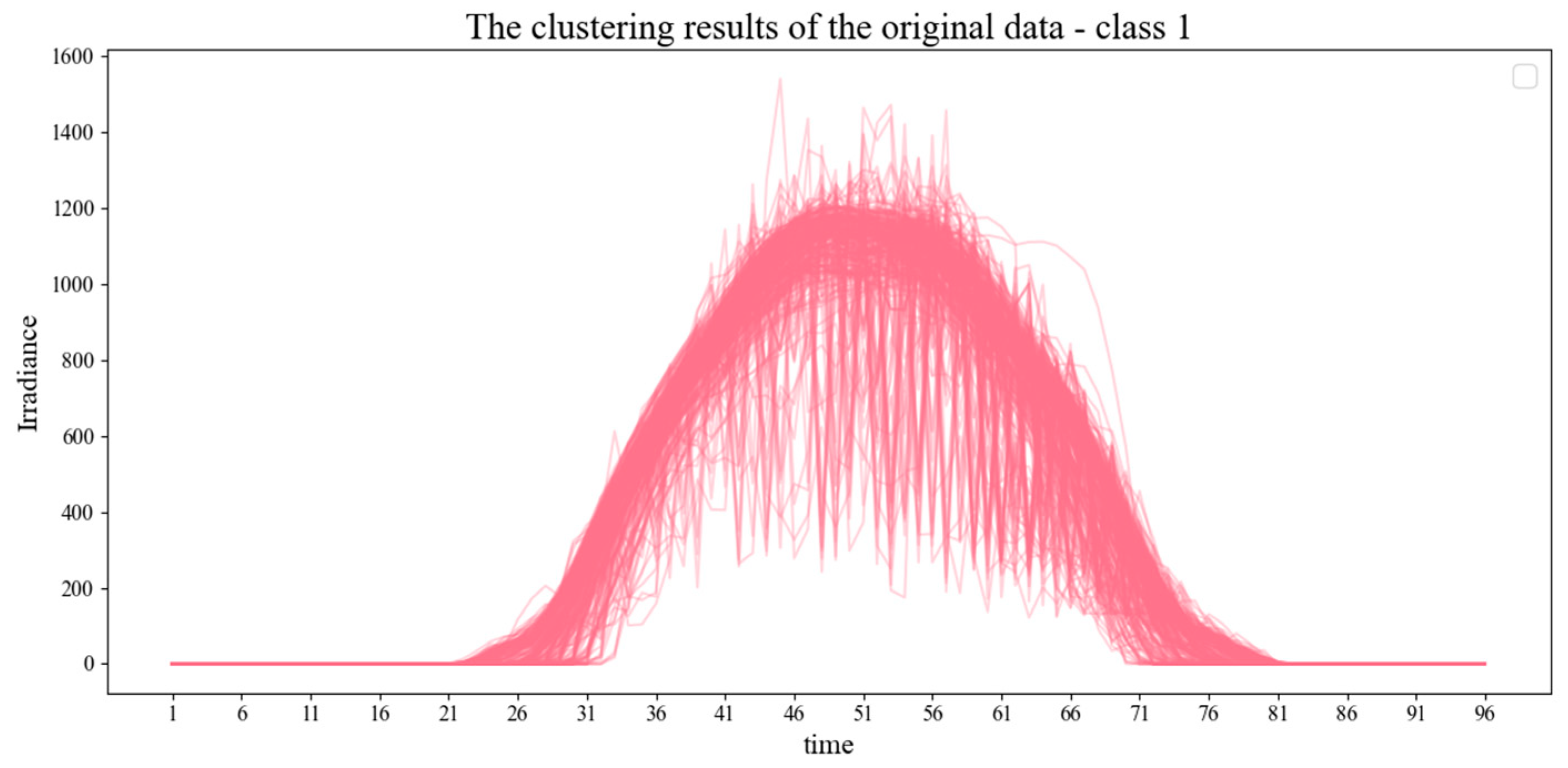
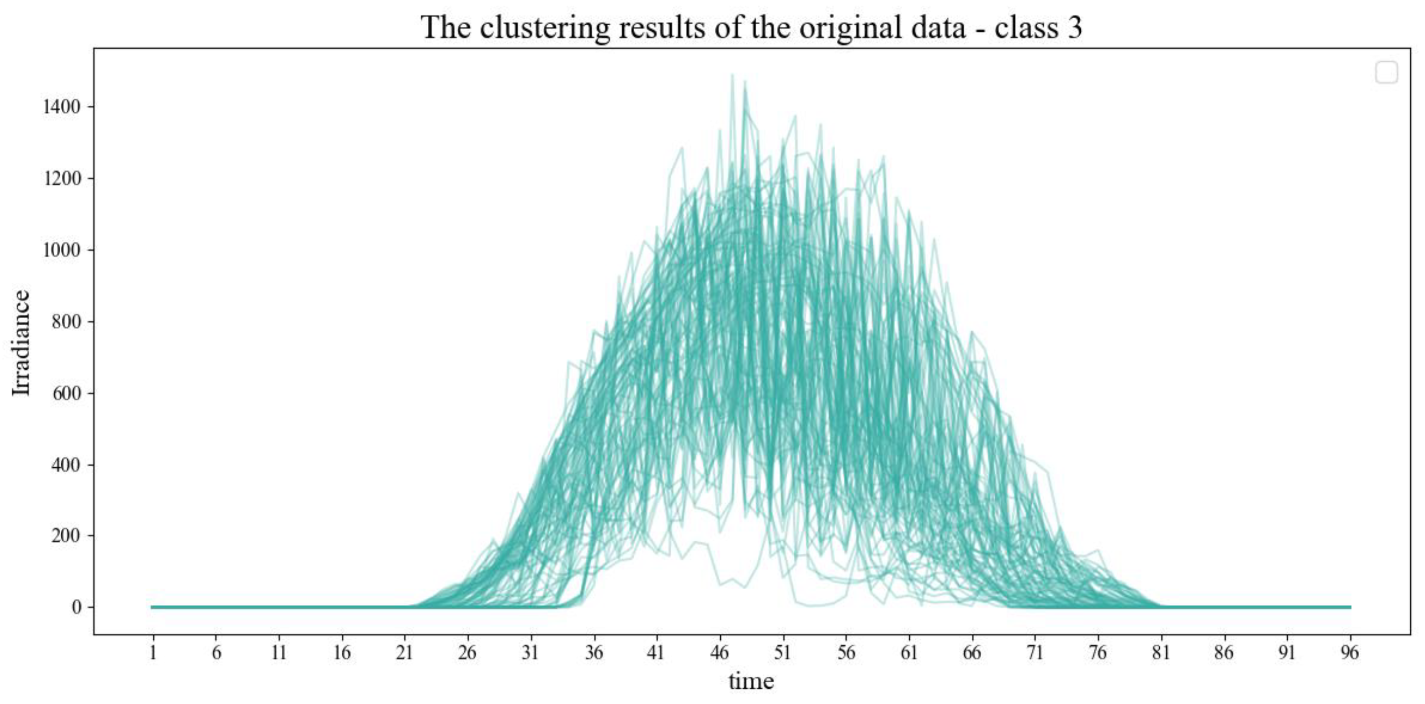
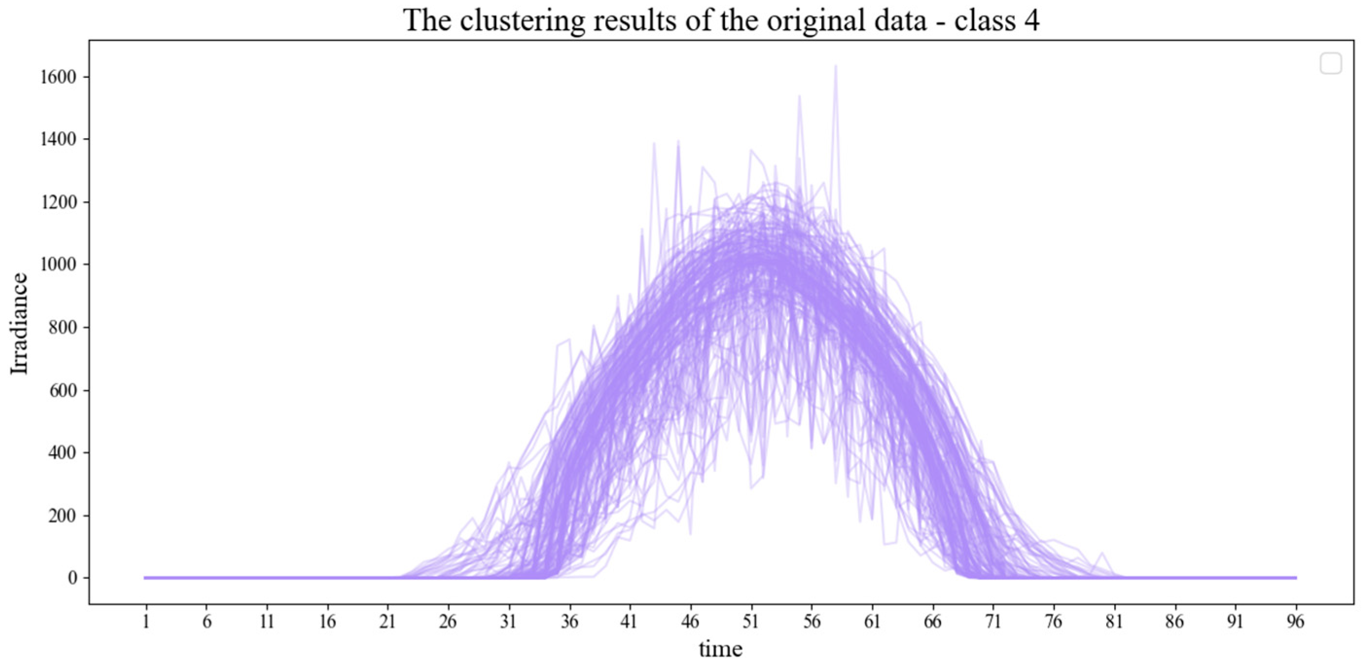
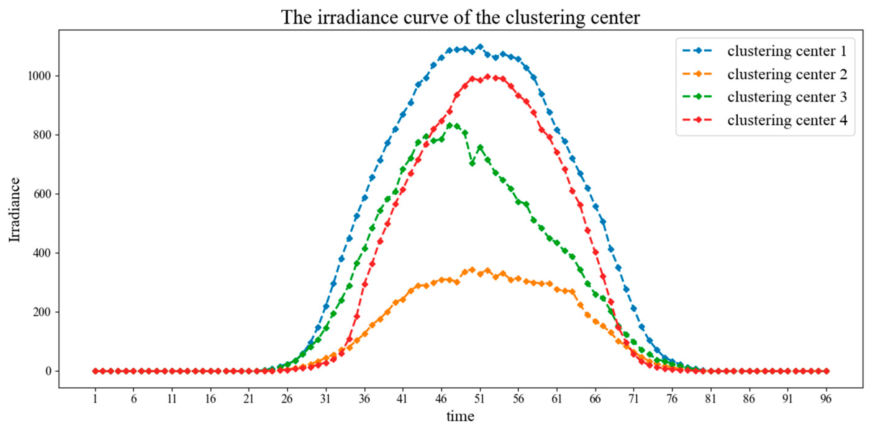
The irradiance curves corresponding to different weather modes have large differences in shape and peak values. In order to distinguish different weather modes every day based on irradiance characteristics and achieve better classification results, K-means clustering was chosen, and the number of clustering categories was 4. The set of daily irradiance profiles for each weather mode after clustering with the clustered center of gravity of the mean daily irradiance pattern is shown in Figure 5, Figure 6, Figure 7, Figure 8 and Figure 9, and the

Table 1. Number of days under each category.

	Cluster 1	Cluster 2	Cluster 3	Cluster 4
Number of days for each category	240	100	91	165

presents the number of dates under each category.

3.3. Results of Numerical Weather Forecast Correction

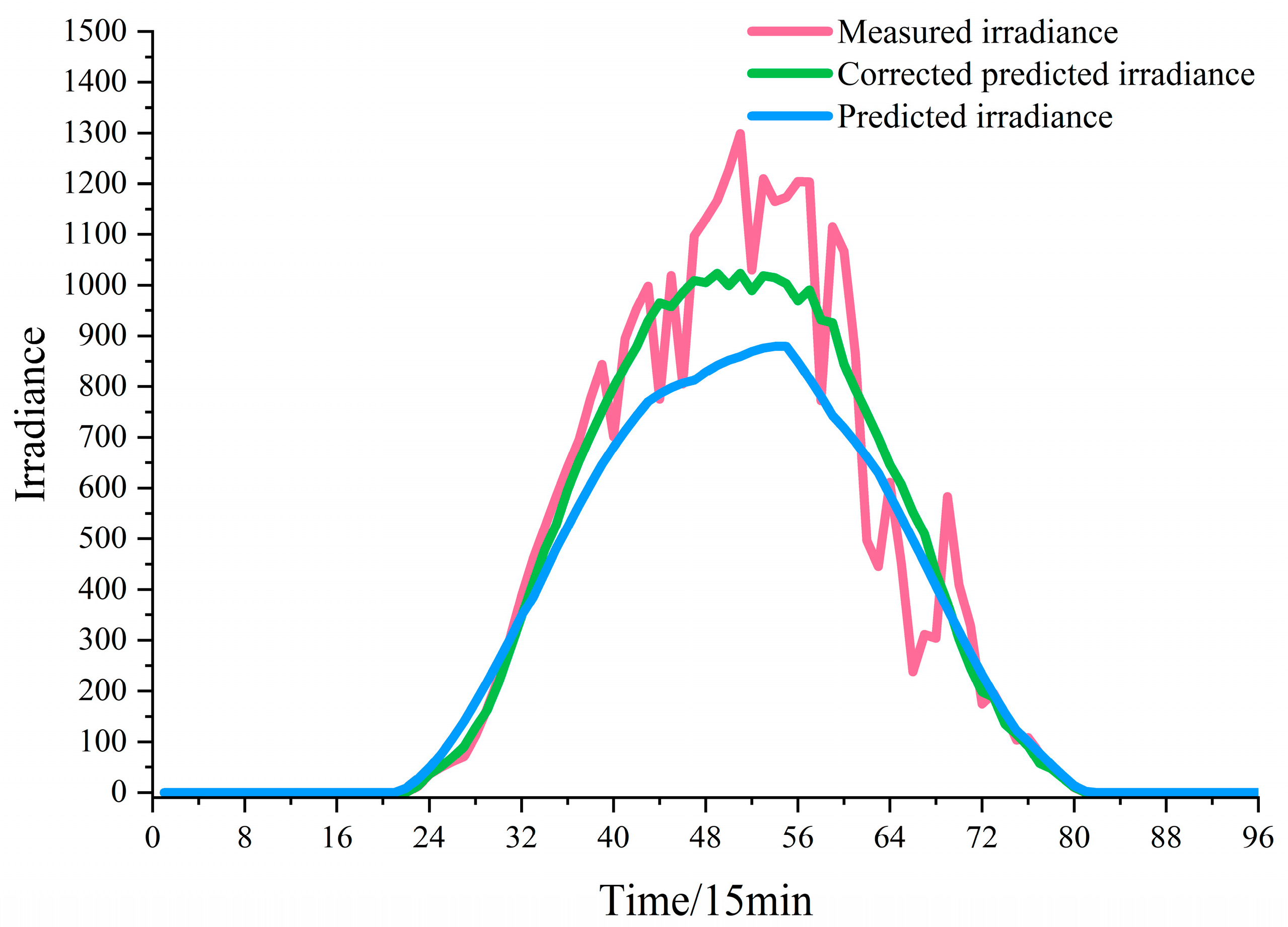
In the second step of numerical weather prediction correction, this study considers the coupling relationship between other meteorological factors and irradiance and selects the GCN model to correct the NWP forecast values of irradiance. The model inputs the NWP forecasts of irradiance, cloudiness, temperature, humidity, wind speed, wind direction, and barometric pressure and calculates the Pearson correlation coefficients between the seven meteorological factors as the adjacency matrix. The target of training is the measured value of irradiance, and the output of the model is the corrected NWP forecast of irradiance. The results after correction of forecast irradiance for the dataset are shown in Figure 10.

3.4. Results of Weather Mode Reliability Prediction

On the basis of obtaining the weather mode classification results and irradiance NWP corrections, we performed plausibility prediction of the test set weather modes. Following the method described in Section 2.3, the labels of the actual weather modes are first encoded, and the values 1,2,3,4 corresponding to the labels class1, class2, class3, and class4 are encoded into the binary numbers of [0,1], [0,1], [0,1], and [0,1], respectively, to be used as the weather mode prediction model’s training output. In the encoded binary numbers, starting from the lowest bit, the value on each digit indicates the probability of belonging to class1, class2, class3, and class4, respectively. Therefore, when training the CNN-based weather mode reliability model, the target output is set in the form of a 4-dimensional vector, and the resultant value of the model output when predicting the test set indicates the reliability level that the day corresponds to each of the four weather modes, i.e., [$p_4$,$p_3$,$p_2$,$p_1$].

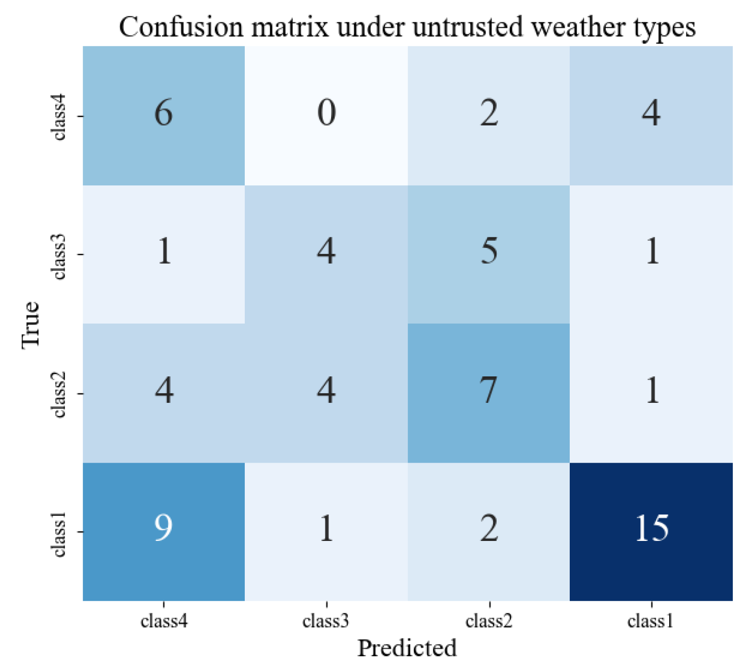
Similar to the irradiance correction model, the input features of the weather mode reliability prediction model are also selected as NWP forecast values for a total of seven meteorological factors: irradiance, cloudiness, temperature, humidity, wind speed, wind direction, and barometric pressure. The difference is that the irradiance forecast values here use the corrected data from the second step, which aims to improve the prediction accuracy of weather modes. To verify the effectiveness of the weather mode reliability prediction method proposed in this paper, the confusion matrices of the weather mode prediction results trusted and untrusted weather are given in Figure 11 and Figure 12, respectively. 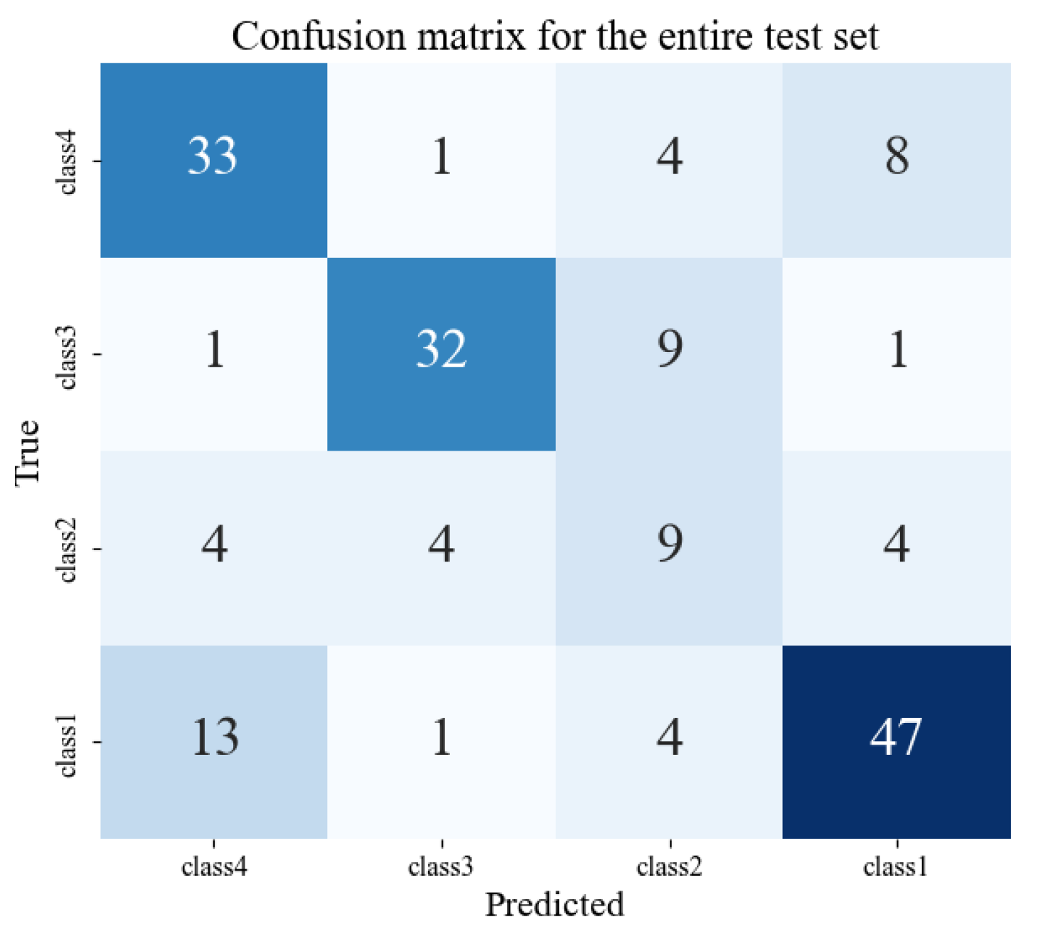And the confusion matrix of the overall weather mode reliability prediction results is given in Figure 13 to calculate the accuracy index. In the simulation, the reliability threshold is set to 0.95, and 60 days in the test set pass the reliability level test and will be predicted using the categorical forecasting strategy, accounting for 49.59% of the total number of days in the test set. Nearly half of the data ensures the significance of the subsequent adoption of the classification forecasting strategy to improve the PV power forecast accuracy. Otherwise, if the number of plausible weather modes is small, the number of days for which a categorical forecast is adopted as a proportion of the entire test set is too low, and the categorical forecasting framework has a limited impact on the overall forecasting accuracy of the prediction.

The overall accuracy and recall of the weather mode prediction results under trusted weather mode, untrusted weather mode, and all weather modes are shown in the

Table 2. Weather mode reliability prediction accuracy rate.

	Class1	Class2	Class3	Class4
Trusted weather mode prediction accuracy rate	82.05%	20%	96.55%	87.10%
Untrusted weather mode prediction accuracy rate	71.43%	43.75%	44.44%	30%
Overall prediction accuracy rate	78.33%	34.62%	84.21%	64.71%

and

Table 3. Weather mode reliability prediction recall rate.

	Class1	Class2	Class3	Class4
Trusted weather mode prediction recall rate	84.21%	40%	87.5%	79.41%
Untrusted weather mode prediction recall rate	55.56%	43.75%	36.36%	50%
Overall prediction accuracy recall rate	72.31%	42.86%	74.42%	71.74%

, and the overall results indicate that the method in this paper is generally able to eliminate many days with incorrectly determined weather modes and improves the robustness of the day-ahead classification prediction framework for PV power generation. However, it is worth noting that the accuracy and recall of class2 are lower than the other weather models due to the small number of days in the test set. Class1 and class4 are also prone to misclassification in weather type prediction due to the main difference between the curve rise and fall periods, and their peaks are very close to each other.

3.5. Results of Photovoltaic Power Classification Forecast

In order to verify the effectiveness of the methods proposed in this paper in improving the accuracy of PV day-ahead power forecast, ablation experiments were conducted to verify the effectiveness of each module in addition to the methods proposed in this paper.

Benchmark method 1: Direct forecast model considering irradiance NWP forecast value correction and not considering weather mode classification.

Benchmark method 2: Classified forecast model without considering irradiance NWP forecast value correction and considering weather mode prediction reliability.

Benchmark method 3: Classified forecast model considering the correction of irradiance NWP forecast values without considering the reliability of the forecast results.

The transformer model was chosen for forecasting in all experiments. The basic configuration of each benchmark and the proposed methods are shown in

Table 4. Basic configuration of benchmark methods in simulation.

Method	Consideration of Classification Forecasting Framework	Consideration of NWP Irradiance Corrections	Consider Weather Mode Prediction Result Decision
Benchmark1 (B1)		√
Benchmark1 (B1)	√		√
Benchmark1 (B1)	√	√
Proposed method (PM)	√	√	√

. The NWP forecast values of irradiance, cloudiness, temperature, humidity, wind speed, wind direction, and barometric pressure are selected as input features to the forecasting models of all methods. The forecast accuracy evaluation metrics for each method are shown in

Table 5. Comparison of PV power forecasting accuracy.

Method	Evaluation Indicators
	eRMSE	eMAE	R
Benchmark1 (B1)	16.64%	8.51%	0.9041
Benchmark2 (B2)	13.24%	6.24%	0.9218
Benchmark3 (B3)	13.37%	6.28%	0.9206
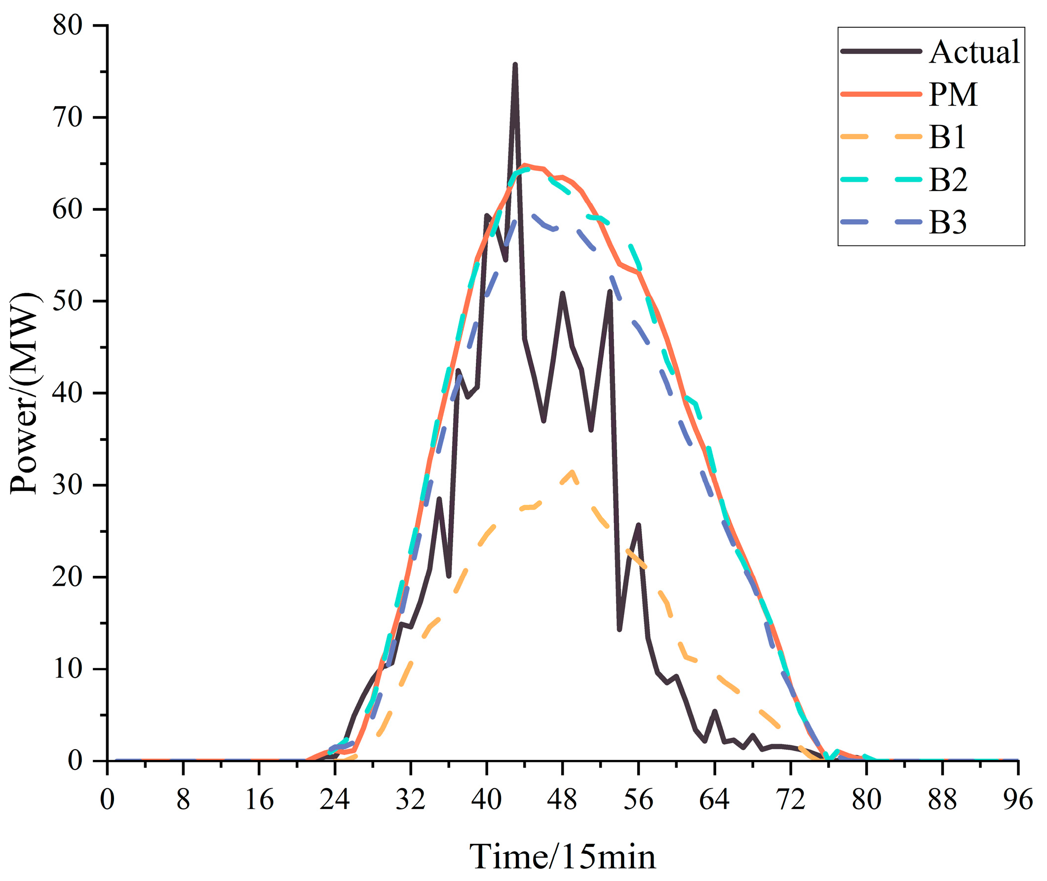
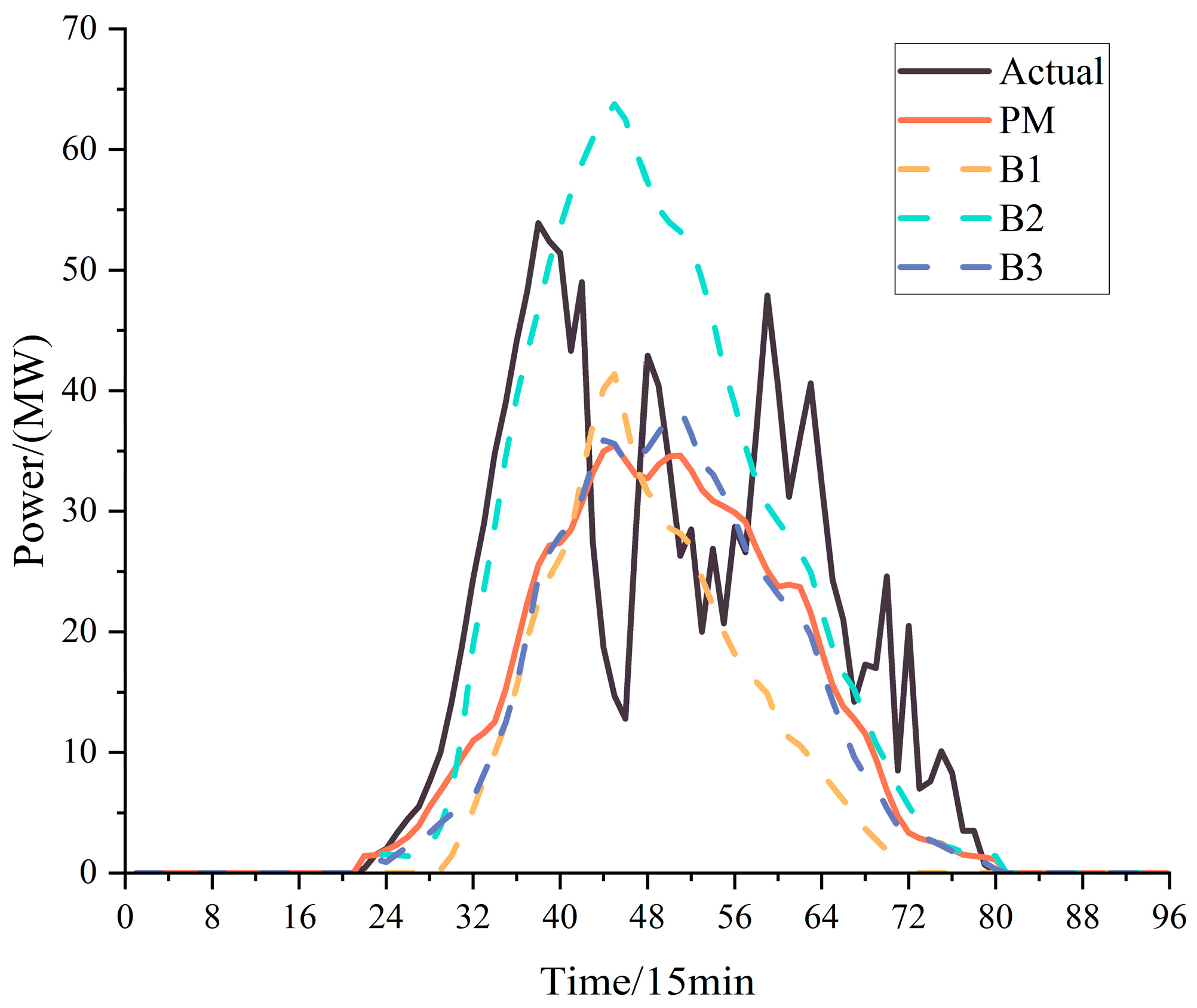
Proposed method (PM)	13.01%	6.20%	0.9246

. The forecasting performance of the entire test set is characterized using eRMSE, eMAE, and the correlation coefficient R. The forecasted results of all the benchmark experiments and the proposed method are collated with the actual output curves according to different weather modes, and the results are shown in Figure 14, Figure 15, Figure 16 and Figure 17.

The results show that the method in this paper outperforms other benchmarks in all evaluation metrics. The accuracy results of benchmark 1 show that the strategy of using classification forecast has a better enhancement effect on improving the forecast accuracy of PV day-ahead output. The proposed method is higher than benchmarks 2 and 3 in terms of accuracy, with an improvement of 0.24%, 0.04%, 0.0028 and 0.37%, 0.08%, 0.004 in terms of eRMSE, eMAE, and R, respectively, but the improvement effect is limited, which is caused on the one hand by the fact that the irradiance forecast value cannot be corrected to the measured irradiance, and there still exists a certain degree of error, on the other hand, the use of the corrected irradiance may lead to a decrease in the correctness of the weather mode reliability prediction, although the correct prediction of the weather mode of the sample days classification forecast improves the accuracy, but because misjudgment of the weather mode for some of the dates in the test set will lead to the selection of the inappropriate classification forecasting model, which will lead to a decrease in the accuracy of the forecast of these days.

4. Conclusions and Discussion

4.1. Conclusions

In this paper, a correction method for the numerical forecast of irradiance considering the weather coupling relationship and a short-term classification forecasting method for PV power based on the correction results of the numerical forecast of irradiance and the weather mode prediction are proposed. In the weather mode classification stage, K-means clustering is used to classify weather modes into four categories based on curve morphology and molecules, which ensures that the classification forecast method is realized based on good weather mode recognition results. In the numerical weather prediction correction stage, the GCN model is used for the irradiance NWP forecast value of the target site, considering the coupling relationship between the various weather elements at the target site, which helps to improve the power forecast accuracy. In the weather mode prediction stage, specific weather modes are translated into the probability of occurrence of various weather modes by means of binary coding. The reliability threshold of the weather mode is used as the basis for the selection of the PV power prediction model by reasonably setting the credibility threshold of the weather type. If the reliability prediction result is accepted, the strategy of classification prediction is adopted, and vice versa, the unified model is adopted.

Compared with the direct forecast weather mode, this method can improve the usability of the weather mode prediction results, and the weather day through the reliability assessment has a higher probability of being predicted correctly, and at the same time, it can provide a reference basis for whether to adopt the weather mode prediction results. In this paper, the reliability assessment mechanism effectively avoids the problem of reduced prediction accuracy due to the wrong prediction of the weather mode and disguises the improvement in the power prediction accuracy, which is very useful for improving the power forecast accuracy under the classification forecast method, which plays an important role in improving the power forecast accuracy.

4.2. Discussion

The reliability of weather models was introduced in this paper to improve the classification forecasting framework, and the experimental results support our proposed improved framework. However, there are still aspects of the proposed forecasting framework that can be improved. There are three main directions for future work:

(1)

In this paper, the weather modes of the field stations are classified by the clustering method of machine learning, but this method is purely mathematical, and in fact, there are clear definitions and distinguishing criteria for different weather modes. In the future, the weather mode classification method can be optimized by combining the machine learning method with the relevant knowledge of meteorology majors.

(2)

The input data used in this paper are only from a single PV plant, and there is a lack of input from neighboring PV plants. In the future, we can consider introducing the data of the neighboring PV plants as the input data of the model to consider the spatial and temporal correlation between irradiance and PV output in the region so as to improve the effect of irradiance correction.

(3)

In this paper, the irradiance forecast accuracy is improved by irradiance numerical forecast correction, which achieves the effect of power forecast accuracy enhancement, but when this paper corrects the original irradiance NWP forecast data, the date to be corrected uses the measured irradiance value on the same day. Therefore, how to correct and improve the irradiance prediction results given by the NWP one day in advance without the actual irradiance measured value in the real situation and further optimize the weather mode reliability prediction and PV power forecast results will be another research direction in the follow-up.