Multiclass Fault Diagnosis in Power Transformers Using Dissolved Gas Analysis and Grid Search-Optimized Machine Learning

Abstract

Dissolved gas analysis remains the most widely utilized non-intrusive diagnostic method for detecting incipient faults in insulating liquid-immersed transformers. Despite their prevalence, conventional ratio-based methods often suffer from ambiguity and limited potential for automation applicrations. To address these limitations, this study proposes a unified multiclass classification model that integrates traditional gas ratio features with supervised machine learning algorithms to enhance fault diagnosis accuracy. The performance of six machine learning classifiers was systematically evaluated using training and testing data generated through four widely recognized gas ratio schemes. Grid search optimization was employed to fine-tune the hyperparameters of each model, while model evaluation was conducted using 10-fold cross-validation and six performance metrics. Across all the diagnostic approaches, ensemble models, namely random forest, XGBoost, and LightGBM, consistently outperformed non-ensemble models. Notably, random forest and LightGBM classifiers demonstrated the most robust and superior performance across all schemes, achieving accuracy, precision, recall, and F1 scores between 0.99 and 1, along with Matthew correlation coefficient values exceeding 0.98 in all cases. This robustness suggests that ensemble models are effective at capturing complex decision boundaries and relationships among gas ratio features. Furthermore, beyond numerical classification, the integration of physicochemical and dielectric properties in this study revealed degradation signatures that strongly correlate with thermal fault indicators. Particularly, the CIGRÉ-based classification using a random forest classifier demonstrated high sensitivity in detecting thermally stressed units, corroborating trends observed in chemical deterioration parameters such as interfacial tension and CO₂/CO ratios. Access to over 80 years of operational data provides a rare and invaluable perspective on the long-term performance and degradation of power equipment. This extended dataset enables a more accurate assessment of ageing trends, enhances the reliability of predictive maintenance models, and supports informed decision-making for asset management in legacy power systems.

1. Introduction

The accelerated expansion of power system infrastructure has significantly increased the global demand for efficient power generation, transmission, and distribution. As a vital component in the power distribution network, the power transformer plays a critical role in maintaining the stability and security of the entire power system [1]. Faults in transformers can result in severe equipment damage and, in extreme cases, may trigger cascading failures across the grid, posing significant risks to national economic stability. A major contributor to early transformer failure is the degradation of the insulating liquid. Studies have indicated that approximately 70–80% of transformer faults are incipient, highlighting the importance of early detection to prevent fault escalation. Timely diagnosis can mitigate fault progression and reduce the likelihood of grid-level failures. Accordingly, the development and implementation of advanced fault diagnosis technologies are essential for improving power system reliability [2,3]. Therefore, a range of diagnostic techniques has been developed to assess and monitor the operational condition of power transformers. Among various diagnostic techniques available, dissolved gas analysis (DGA) is one of the most established and widely adopted techniques for detecting incipient faults and assessing the operational status of power transformers [3]. This technique involves detecting and monitoring the concentration of combustible and fault-related gases dissolved in the insulating liquid of transformers. These gases include hydrogen (H₂), methane (CH₄), ethylene (C₂H₄), ethane (C₂H₆), acetylene (C₂H₂), carbon monoxide (CO), and carbon dioxide (CO₂). Variation in these gas levels typically indicates the onset or progression of internal faults within the transformer [2,4]. Therefore, the type and the concentration of the dissolved gases are crucial in identifying and classifying specific types of faults. Gas chromatography is an analytical technique commonly used to separate and analyse these gases, relying on differences in their flow rates through a stationary phase [3]. Based on this principle, several conventional diagnostic approaches have been developed, which are classified into three main categories. These categories are the key gas method, the gas generation rate method, and the gas ratio method [2].

Conventional gas ratio techniques, such as the IEC ratio method (IRM), Rogers ratio method (RRM), Doernenburg ratio method (DRM), CIGRÉ method, and Duval triangle, have long been used in the industry for transformer fault diagnosis. However, despite their widespread adoption, these methods often suffer from limited diagnostic accuracy, particularly when multiple gases are involved or when the gas ratio falls near critical threshold boundaries. Also, the precision of fault analysis tends to decrease as the classification schemes become more granular, while overly broad classifications can obscure critical distinctions, thereby hindering effective fault identification. These challenges are exacerbated by the nonlinear behaviour of gas generated, which does not follow a simple relationship with transformer operating ageing indicators such as interfacial tension and acidity. Also, the imbalanced, insufficient, and overlapping state of gas-decomposed DGA datasets remains a significant limitation to the development and deployment of robust and accurate diagnostic approaches [1,5]. To address these challenges, machine learning (ML) has gained increasing attention for its ability to model complex, nonlinear relationships and generalize from historical DGA data. In many ML-based frameworks, conventional gas ratio schemes and graphical interpretations are used as input features, allowing the automated and data-driven classification of fault types [1,2]. A fault detection model based on the K-nearest neighbours (KNN) and decision tree (DT) was presented in [6] using the New York Power Authority dataset. The model initially employs key gas methods to identify outliers, followed by the application of the basic gas ratio method for fault classification. The approach proposed achieved an accuracy of 88%, demonstrating its effectiveness in detecting transformer faults based on DGA data. The research in [7] evaluates a hybrid diagnostic model that combines particle swarm optimization-tuned support vector machine (SVM) with the KNN framework. This model was integrated with the Duval Pentagon method to enhance transformer fault classification based on DGA. The proposed approach was tested against five distinct fault types detectable in insulating liquid and achieved a diagnostic accuracy of 88%. A diagnostic model was proposed in [8] that integrated the SVM algorithm to assess the severity of transformer faults. This approach enhances traditional graphical analysis by incorporating gas concentration levels, gas generation rates, and standard DGA interpretation results into a unified diagnostic framework. The model demonstrated a diagnostic accuracy of 88%, indicating its effectiveness in providing a quantitative assessment of transformer fault conditions. In [9], the authors proposed a hybrid fault diagnostic method based on the DGA dataset collected from the Agilent chemical laboratory. The approach integrates an SVM optimized using the Bat algorithm with Gaussian classifiers to enhance diagnostic performance. This coupled system aims to improve classification accuracy by combining the optimization capabilities of the Bat algorithm with the generalization strength of SVM and the probability modeling of Gaussian classifiers. The proposed model achieved a diagnostic accuracy of 93.75%, indicating a significant improvement over the conventional method.

In general, the recent systematic survey in [1] revealed that the majority of research efforts on transformer fault classification using DGA predominantly employed ML algorithms such as SVM, Artificial Neural Network (ANN), and KNN, with usage rates of approximately 32%, 17%, and 12%, respectively. These algorithms demonstrated considerable effectiveness in identifying and classifying fault types based on gas concentration patterns, owing to their ability to model complex nonlinear relationships and generalize from limited datasets. However, each technique has inherent limitations. SVM often requires careful parameter tuning and may not scale efficiently with large datasets. ANN demands substantial computational resources and large volumes of labelled data for effective training, which may not always be available in practical cases. Similarly, the performance of KNN is highly sensitive to the choice of distance metric and the selection of the parameter K. Also, its use can be computationally intensive during the prediction stage, as comparison with all training samples is required to determine the nearest neighbours. These drawbacks highlight the need for ongoing research into more advanced and efficient diagnostics frameworks. Therefore, beyond SVM and KNN, this study investigates the application of ensemble ML models across four widely accepted DGA diagnostic ratio schemes to enhance transformer fault classification performance. The performance of each model was evaluated using six key metrics to ensure a comprehensive assessment. In addition, to enhance the reliability and generalizability of the results, a 10-fold cross-validation strategy was employed with grid search optimization for hyperparameter tuning and optimal model selection. Comparative analysis was conducted to highlight the strengths and limitations of each model across different diagnostic schemes, providing valuable insights into their suitability for real-world deployment. Furthermore, key physicochemical and dielectric properties are incorporated to enable the more comprehensive interpretation of fault types beyond numerical classification. Therefore, this study not only compares model performance across different diagnostic schemes but also emphasizes the diagnostic significance of insulation liquid degradation trends and their correspondence with ML-based fault predictions.

2. Materials and Methodology

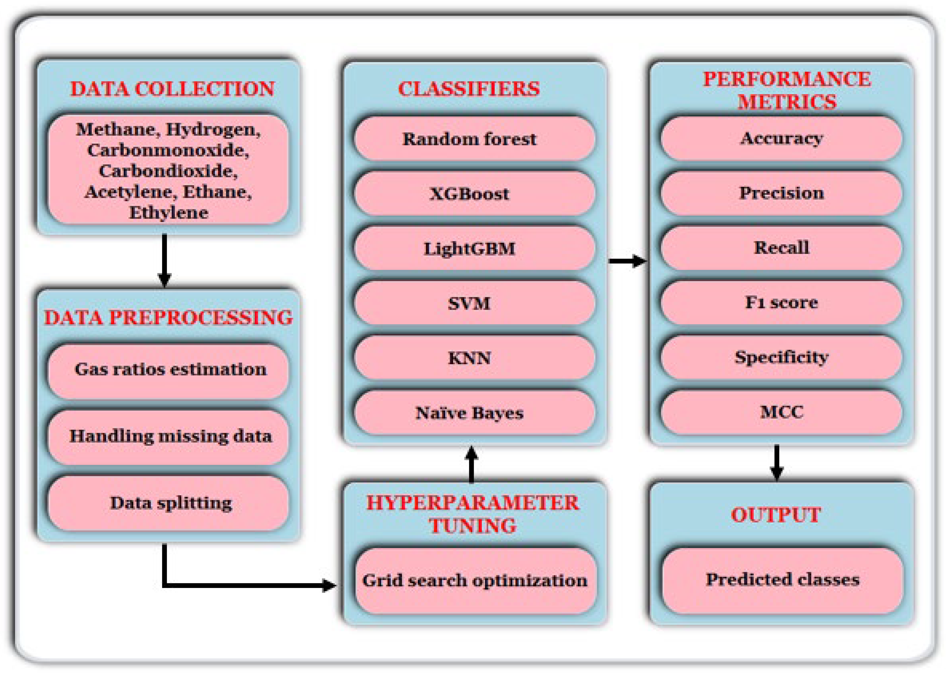
The DGA dataset employed in this study was collected from Rio Tinto, Saguenay, Canada, comprising 1702 records obtained between 2010 and 2024. The complete data entries were partitioned using an 80:20 train–test split, where 80% of the data was used for training and the remaining 20% was used for testing. This is a common and experimentally validated practice for ensuring robust model assessment. Simulations were conducted using six different ML models, and their performance was assessed based on standard evaluation metrics. Furthermore, to enable the ML models to process categorical output values, label encoding was applied to the multiclass target variable. This technique converts non-numerical forms of data by assigning each unique point a value between 0 and n_classes − 1, where n_classes represents the total number of distinct categories in the target variable. Also, the computational implementation was carried out on a system equipped with a Core i5 processor (1.8 GHz, 4 cores, 6 MB cache, 64-bit architecture, 8 GB RAM). It ran Windows 10 (64-bit) and utilized Python 3.9 libraries such as Scikit-learn, Pandas, NumPy, Matplotlib, and Seaborn.

Table 1. A sample of the DGA dataset.

S/N	H2	CH4	CO	CO2	C2H4	C2H6	C2H2
1	96	409	178	2634	1522	218	10
2	35	70	365	3225	179	30	2
3	35	61	327	3096	188	25	1
4	26	48	470	4337	179	25	2
5	30	195	85	1706	908	148	4
…	…	…	…	…	…	…	…
341	3	3	128	815	11	1	3
342	50	30	976	8015	171	22	4
343	14	7	713	3042	60	1	7
344	9	3	274	2629	6	1	1
345	19	6	338	3640	21	1	20
…	…	…	…	…	…	…	…
682	16	3013	9	485	67041	8193	2321
683	14	41	201	3762	173	26	1
684	10,447	2515	74	291	3734	116	28,639
685	1747	216	185	1789	11	82	1
686	29	5	451	2680	64	3	1
…	…	…	…	…	…	…	…
1021	11	6	429	2278	20	6	1
1022	18	33	354	3206	107	20	2
1023	16	45	1966	7783	37	11	3
1024	146	122	1041	5168	254	46	7
1025	79	81	1651	10,241	202	44	3
…	…	…	…	…	…	…	…
1698	37	36	571	5537	136	29	2
1699	3	12	5	300	92	13	35
1700	1653	740	104	600	2048	179	5812
1701	51	9	656	2847	62	4	2
1702	18	6	592	7279	22	1	1

presents a sample of the DGA dataset, and a detailed flow diagram illustration of the methodology process is presented in Figure 1.

In addition, a total of 50 power transformers, with some over 80 years old and originating from various manufacturers, were studied as part of a long-term condition monitoring initiative by the Canadian utility Rio Tinto. These transformers, rated between 13.8 kV and 173 kV, were originally installed and commissioned between 1930 and 2022. Over the years, insulating oil samples were periodically collected and analyzed to assess their electrical, chemical, and physical properties. This analysis, carried out from 1930 through to 2022, provides valuable insight into the ageing behaviour and operational condition of the service-aged transformer oils. The data include key physicochemical and dielectric parameters such as breakdown voltage (BDV), interfacial tension (IFT), acid value, moisture content, and CO₂/CO ratio. For systematic analysis, the transformers were categorized into four voltage classes. The voltage classes are as follows: 13.8 kV with 11 units, 154 kV with 11 units, 161 kV with 22 units, and 173 kV with 6 units. The collected physicochemical and dielectric parameters data were subsequently compared with the diagnostic outputs of the best-performing ML classifier under each gas ratio scheme. This comparison is designed to systematically identify consistencies or discrepancies between the observed chemical degradation trends and fault types predicted by ML classifiers. Furthermore, this study presents practical insights gained from decades of operating ageing power equipment, with particular emphasis on units that have remained in continuous service for over 80 years.

2.1. Diagnostic Techniques

Several DGA interpretation methods have been developed to identify and classify faults in power transformers. Among the most widely employed are the ratio-based diagnostic methods, which analyse the relationship between specific dissolved gas concentrations to infer the presence and type of fault. In this study, four methods are considered, which are grounded in international standards and expert guidelines.

The Doernenburg ratio method (DRM) is based on the IEEE C57.104 standard and employs four key gas ratios to diagnose transformer faults. This method demonstrated the effectiveness of identifying various fault types, including thermal decomposition, partial discharge, and arcing, as illustrated in

Table 2. DRM-specific threshold limits for each gas ratio.

Fault Type	${\mathbf{R}}_1 = \frac{\mathbf{C}{\mathbf{H}}_4}{{\mathbf{H}}_2}$	${\mathbf{R}}_2 = \frac{{\mathbf{C}}_2{\mathbf{H}}_2}{{\mathbf{C}}_2{\mathbf{H}}_4}$	${\mathbf{R}}_3 = \frac{{\mathbf{C}}_2{\mathbf{H}}_2}{\mathbf{C}{\mathbf{H}}_4}$	${\mathbf{R}}_4 = \frac{{\mathbf{C}}_2{\mathbf{H}}_6}{{\mathbf{C}}_2{\mathbf{H}}_2}$
Thermal decomposition	>1	<0.75	<0.3	>0.4
Partial discharge	<0.1	Not significant	<0.3	>0.4
Arcing	0.1–1.0	>0.75	<0.3	<0.4

[10,11].

The Rogers ratio method (RRM), also derived from the IEEE C57.104 standard, relies on three specific gas ratios, as shown in

Table 3. RRM-specific threshold limits for each gas ratio.

Fault Type	${\mathbf{R}}_1 = \frac{\mathbf{C}{\mathbf{H}}_4}{{\mathbf{H}}_2}$	${\mathbf{R}}_2 = \frac{{\mathbf{C}}_2{\mathbf{H}}_2}{{\mathbf{C}}_2{\mathbf{H}}_4}$	${\mathbf{R}}_5 = \frac{{\mathbf{C}}_2{\mathbf{H}}_4}{{\mathbf{C}}_2{\mathbf{H}}_6}$
Normal	0.1–1.0	<0.1	<1.0
Low-energy-density arcing- PD	<0.1	<0.1	<1.0
Arcing–High-energy discharge	0.1–1.0	0.1–3.0	>3.0
Low-temperature thermal fault	0.1–1.0	<0.1	1.0–3.0
Thermal fault, T < 700 °C	>1.0	<0.1	1.0–3.0
Thermal fault, T > 700 °C	>1.0	<0.1	>3.0

[10,11]. These ratios were selected based on practical industry experience and their relevance in diagnosing common transformer fault scenarios. Unlike some diagnostic methods, RRM is applied when individual gas concentrations exceed prescribed thresholds and do not require predefined minimum limits for valid fault interpretation [12].

The IEC ratio method (IRM) follows a similar approach to RRM as it utilizes three key gas ratios to diagnose transformer faults, as outlined in

Table 4. IRM-specific threshold limits for each gas ratio.

Fault Type	${\mathbf{R}}_1 = \frac{\mathbf{C}{\mathbf{H}}_4}{{\mathbf{H}}_2}$	${\mathbf{R}}_2 = \frac{{\mathbf{C}}_2{\mathbf{H}}_2}{{\mathbf{C}}_2{\mathbf{H}}_4}$	${\mathbf{R}}_5 = \frac{{\mathbf{C}}_2{\mathbf{H}}_4}{{\mathbf{C}}_2{\mathbf{H}}_6}$
Partial discharge	<0.1	Not significant	<0.2
Low-energy discharge	0.1–0.5	>1.0	>1.0
High-energy discharge	0.1–1.0	0.6–2.5	>2.0
Thermal fault, T < 300 °C	>1.0	Not significant	<1.0
Thermal fault, 300 °C < T < 700 °C	>1.0	<0.1	1.0–4.0
Thermal fault, T > 700 °C	>1.0	<0.2	>4.0

[10,11]. This method is particularly effective in identifying thermal faults across a range of temperature levels (300–700 °C), as well as four categories of electrical faults, which include normal ageing, partial discharges, and both low-energy and high-energy discharges [12].

The CIGRÉ method offers diagnostic criteria for interpreting DGA results based on expert knowledge and field experience. Unlike other methods, it employs five gas ratios to identify faults such as partial discharges, arcing, thermal faults, overheating in paper, and cellulosic degradation by electrical faults. The interpretation scheme for this method is presented in

Table 5. CICRÉ-specific threshold limits for each gas ratio.

Fault Type	Ratio	Limit
Arcing	$C_1={\displaystyle \frac{{\mathrm{C}}_2{\mathrm{H}}_2}{{\mathrm{C}}_2{\mathrm{H}}_6}}$	≥1.0
Partial discharges	$C_2={\displaystyle \frac{{\mathrm{H}}_2}{\mathrm{C}{\mathrm{H}}_4}}$	≥10.0
Thermal fault	$C_3={\displaystyle \frac{{\mathrm{C}}_2{\mathrm{H}}_4}{{\mathrm{C}}_2{\mathrm{H}}_6}}$	≥1.0
Discharges in OLTC	$C_4={\displaystyle \frac{{\mathrm{C}}_2{\mathrm{H}}_2}{{\mathrm{H}}_2}}$	≥2.0
Overheating, paper	$C_5={\displaystyle \frac{{\mathrm{C}\mathrm{O}}_2}{\mathrm{C}\mathrm{O}}}$	≥10.0
Cellulosic degradation by electrical fault	$C_5$	<3.0

[10,11].

2.2. ML Frameworks

In this study, classical and ensemble machine learning algorithms were selected due to their proven accuracy, interpretability, and computational efficiency when applied to structured tabular data such as that derived from DGA. These models are well-suited for multiclass classification tasks, handle moderate-sized datasets effectively, and require neither extensive hardware nor a complex training procedure. Furthermore, ensemble models are more appropriate for deployment in practical, real-time fault detection systems given their speed, robustness, support for missing values, and ability to generate feature importance scores, thus aligning better with our goal of developing a high-performance, interpretable, and deployable diagnostic framework [13].

2.2.1. Random Forest

Random forests (RFs), also known as random decision forests, are a robust ensemble learning technique that can be applied to both classification and regression tasks. They operate by constructing multiple independent decision trees during training, and for classification tasks, the final prediction is determined by aggregating the predictions of all the trees through majority voting. This approach effectively mitigates the overfitting commonly associated with single decision trees by introducing randomness in both feature selection and data sampling. Although random forests may not achieve the peak accuracy of more complex models like gradient boosting methods, they offer a strong balance of performance, interpretability, and efficiency. Due to their versatility and low pre-processing requirements, random forests are widely used in practice, often serving as reliable black box models that perform well across diverse datasets [14]. In multiclass classification tasks, random forest evaluates all the classes simultaneously within each tree, rather than training separate trees for each class. The class prediction for a data sample is given by (1), and the model minimizes the objective function (2) during training:

$$\widehat{y}=arg \underset{c}{\text{max}}\sum _{t=1}^{T}I\left(h_t\left(x\right)=c\right)$$

(1)

$$L={\displaystyle \frac{1}{N}}\sum _{i=1}^N{\left(y_i-\widehat{y_i}\right)}^2$$

(2)

where $\widehat{y_i}$ denotes the predicted value, $y_i$ is the actual value, $T$ is the total number of decision trees, and $h_t\left(x\right)$ denotes the class predicted by the $t$-th tree.

2.2.2. XGBoost

Extreme gradient boosting (XGBoost) is a tree-based ML algorithm that has recently gained significant popularity for classification tasks due to its high effectiveness and scalability [15]. It is an end-to-end gradient boosting framework designed to efficiently handle both classification and regression problems. The model is chosen for its numerous advantages, including the ability to learn from previous errors, fine-tune a wide range of hyperparameters, handle imbalanced datasets, and process missing values. As a boosting algorithm, XGBoost builds an ensemble of weak learners sequentially, with each new tree aiming to correct the errors of the previous ones. As a result, it enhances prediction accuracy by optimizing the gain from prior predictions. In multiclass classification tasks, XGBoost enhances decision-making by minimizing the log-loss function for each class, as defined in (3):

$$L=\sum _{i=1}^n\sum _{k=1}^K{y}_{ik}\text{log} p_{ik}$$

(3)

where $y_{ik}$ indicates whether the $i$-th instance belongs to class $k$, and $p_{ik}$ is the predicted probability of that instance belonging to class $k$.

2.2.3. LightGBM

The light gradient boosting machine (LightGBM) is an advanced gradient-boosting decision tree framework that supports parallel training, offering significant advantages in terms of computational speed, model stability, and low memory usage. It can efficiently handle large-scale and high-dimensional datasets. Unlike traditional gradient boosting methods, LightGBM is built on a histogram-based algorithm, which improves training speed and reduces memory consumption by grouping continuous feature values into discrete bins [16]. In general, the key features of LightGBM include depth-constrained leaf-wise tree growth for improved accuracy, one-sided gradient sampling to reduce data complexity and accelerate training, and support for parallel and GPU-accelerated learning. Furthermore, the objective function in LightGBM combines the loss function, a regularization term, and an additional constant component, as shown in (4). The loss function is minimized iteratively by adjusting the weights of the training instances, allowing each subsequent tree to focus on the instances that were misclassified by the previous tree [17].

$$obj\left(t\right)=L\left(t\right)+\mathit{\Omega }\left(t\right)+c$$

(4)

where $L\left(t\right)$ is the loss function; $\mathit{\Omega }\left(t\right)$ is the regularization term, penalizing model complexity; and $c$ is a constant term.

2.2.4. SVM

Support vector machines (SVMs) are sparse, kernel-based classifiers that construct decision boundaries using only a subset of the training data, known as support vectors, which define the margins of the separating hyperplane. They operate based on the structural risk minimization principle to find the best hyperplane for separating two classes in the input space [18]. Although the entire training set must be available during model fitting, only support vectors are retained for prediction, thereby reducing the computational complexity and storage requirements. The number of support vectors is data-dependent and reflects the underlying complexity of the dataset. SVMs solve a convex optimization problem regularized by a margin maximization constraint, which promotes better generalization by positioning the decision boundary at the maximum possible distance from the closest training samples of each class. For nonlinearly separable data, SVMs employ the kernel trick to project the input data into a higher-dimensional feature space, where a linear separator can effectively discriminate between classes. The choice of kernel function and its parameters is therefore critical to model performance as the effectiveness of SVM principally depends on the size and density of the kernel [2,19]. SVM determines the optimal hyperplane for class separation using (5).

$$f\left(x\right)=sign\left(w^{T}x+b\right)$$

(5)

where $f\left(x\right)$ is the output of the SVM decision function $w$ is the weight vector that determines the orientation of the hyperplane, $x$ is the input feature vector, and $b$ is the bias term that adjusts the hyperplane (decision boundary) [20].

2.2.5. KNN

K-nearest neighbour (KNN) is a versatile, non-parametric algorithm applicable to both classification and regression tasks [15]. Unlike other conventional machine learning techniques that require training to build a predictive model, KNN operates in a model-free fashion. It makes a decision solely based on the relationships between data points. When a new data point needs to be classified, KNN calculates its distance to all existing samples in the training dataset. Based on these computations, it determines the k-nearest data points, those that exhibit the greatest similarity to the test instance, based on a chosen distance metric. The class label assigned to the test sample corresponds to the majority class among these k-nearest neighbours. The algorithm’s performance principally depends on two factors, which are the value of k and the distance metric. The value of k is typically selected through empirical testing. A small k can lead to overfitting, making the model too sensitive to noise in the data, while a large k results in underfitting by smoothing out important local patterns and blurring class distinctions. The distance metric determines how similarity is quantified between data points. While several metrics, such as Euclidean, Minkowski, Manhattan, and Chebyshev, exist [21], Euclidean is selected in this study. The Euclidean distance $d\left(x,y\right)$ between two samples $x$ and $y$ is computed as follows:

$$d\left(x,y\right)=\sqrt{\sum _{k=1}^n{\left(x_{ik}-y_{jk}\right)}^2}$$

(6)

where n is the number of features, and $x_{ik}$ and $y_{jk}$ represent the $k$-th feature values of the $i$-th and $j$-th data points, respectively [20].

2.2.6. Naïve Bayes

The Naïve Bayes algorithm operates by calculating the probabilities of events occurring within a dataset to support decision-making [3]. It evaluates the likelihood of each target attribute value in a data sample and classifies the sample, establishing the class with the highest probabilities. Furthermore, the algorithm assumes that all the features contribute equally and independently to the classification decision. While this assumption enhances computational efficiency, it can make Naïve Bayes less suitable for real-world problems where feature interdependencies exist [22]. In addition, the Gaussian-type Naïve Bayes classifier, which minimizes variation within attributes, was employed in this study using the sklearn model modules.

3. Optimization and Evaluation

3.1. Grid Search Optimization

Before training the ML models, the hyperparameter values must be defined before learning. These control the training process, unlike model parameters like weights, which are learned from data. Choosing optimal hyperparameters is crucial for model performance, and since these values can vary significantly across datasets, manual tuning can be challenging. To address this, grid search, which is an automated hyperparameter optimization technique, is employed. Grid search is a comprehensive method for hyperparameter tuning that systematically explores all possible combinations within a defined parameter space. Its primary strength lies in its exhaustiveness, ensuring that the most optimal hyperparameter set is identified, provided it exists within the specified range [18]. In addition, its simplicity and clarity make it easy to implement and interpret, especially in scenarios involving relatively small-parameter grids. Grid search optimizes the model parameters, employing a cross-validation method as a performance metric. It systematically explores all possible combinations of hyperparameter values defined in a grid configuration. The aim is to identify the optimal hyperparameter combination so that the classifier can predict unknown data accurately. For each configuration, the model’s performance is assessed on a held-out validation set derived from the training data. The grid search algorithm identifies and selects the hyperparameter combination that yields the best validation performance. The final model is then retrained using the full training data and the optimal hyperparameters, determined during the search process [21]. The model’s parameter optimization, performed using grid search, is illustrated in Figure 2, while the optimal parameters for each model are presented in

Table 6. Optimal hyperparameter with grid search tuning.

Model	Hyperparameter	Configuration Domain	Optimal Tuning
Random forest	n_estimators	50, 100, 200	100
	max_depth	None, 10, 20, 30	10
	min_samples_split	2, 5, 10	5
	min_samples_leaf	1, 2, 4	1
XGBoost	n_estimators	50, 100, 200	200
	max_depth	3, 6, 10	6
	learning rate	0.01, 0.1, 0.2	0.1
	subsample	0.7, 0.8, 1.0	0.8
LightGBM	n_estimators	50, 100, 200	200
	num_leaves	31, 50, 100	50
	learning rate	0.01, 0.1, 0.2	0.01
SVM	C	0.1, 1, 10	1
	kernel	linear, rbf, poly	rbf
	gamma	scale, 0.001, 0.01	scale
KNN	n_neighbors	3, 5, 7	5
	weight	uniform, distance	uniform

.

3.2. K-Fold Cross-Validation

Cross-validation (CV) is a statistical technique widely used to evaluate the generalization performance of machine learning models. Unlike repeated random subsampling, it partitions the dataset into non-overlapping subsets in a systematic manner [23]. In this study, the value of K = 10, resulting in a 10-fold CV, was employed. The value of K is carefully selected based on thorough experimental evaluation to ensure optimal model performance. Overall, 10-fold CV is particularly effective for evaluating predictive models, providing a robust estimate of their real-world performance [14]. The dataset is partitioned into ten equal folds (subsets) in each iteration, where one fold serves as the validation set while the remaining nine (K − 1) are used for training. This process is repeated ten times, ensuring that each data point is used exactly once for validation. Figure 3 illustrates the standard 10-fold cross-validation procedure.

3.3. Performance Metrics

Assessing the performance of a classification model is a critical step in validating the model’s reliability, achieved by comparing the model’s predicted outputs against the actual values observed. It requires more than just estimating the overall accuracy, particularly in cases involving class imbalance or a multiclass classification prediction, such as transformer fault diagnosis. An extensive assessment involves several metrics that capture different aspects of prediction quality, including the model’s capacity to correctly identify both positive and negative instances, handle misclassification, and maintain robustness across varying class distributions. In this regard, six metrics are employed in this study to provide deeper insight into the classifier’s strengths and limitations, enabling a more reliable and interpretable evaluation of its predictive abilities.

Accuracy, computed using (7), measures the overall effectiveness of the model by calculating the proportion of correctly classified instances (both positive and negative) out of the total predictions. Precision, computed using (8), measures the proportion of true positive predictions among all the predicted positives. It indicates how many positive predictions were correct. Recall is computed using (9) to measure the proportion of actual positives correctly identified by the model. It reflects the model’s capacity to capture all positive instances. It is serves as the sensitivity of the model regarding binary classification. The F1 score computed using (10) is the harmonic mean of precision and recall. It provides a balanced measure that accounts for both false positives and false negatives, which is especially useful when class distribution is imbalanced [24]. Specificity, the counterpart to recall, measures the proportion of actual negatives that were correctly classified. It is estimated using (11). Matthews correlation coefficient (MCC), computed using (12), is a balanced metric that takes into account all four confusion matrix components, which are TP, TN, FP, and FN. It is particularly useful for classification with imbalanced classes. The MCC offers a balanced evaluation metric that maintains strong discrimination power, consistency, and coherence, even in the presence of varying class distributions and multiple fault categories [25].

$$Accuracy={\displaystyle \frac{TP+TN}{TP+TN+FP+FN}}$$

(7)

$$Precision={\displaystyle \frac{TP}{TP+FP}}$$

(8)

$$Recall={\displaystyle \frac{TP}{TP+FN}}$$

(9)

$$F1 score=2\times {\displaystyle \frac{Precision\times Recall}{Precision+Recall}}$$

(10)

$$Specificity={\displaystyle \frac{TN}{TN+FP}}$$

(11)

$$MCC={\displaystyle \frac{TN\times TP-FN\times FP}{\sqrt{\left(TP+FP\right)\left(TP+FN\right)\left(TN+FP\right)\left(TN+FN\right)}}}$$

(12)

where false positive (FP) represents the number of instances that the model incorrectly labels as belonging to the positive class when they are negative; false negative (FN) refers to cases where the model predicts a negative class, but the actual class is positive; true positive (TP) is the number of instances correctly predicted as belonging to the positive class; true negative (TN) is the number of instances correctly predicted as belonging to the negative class [14,21,25].

3.4. Confusion Matrix

A confusion matrix is an arithmetically derived tool used for evaluating a model’s classification performance. It provides a detailed, holistic view of how well the classifier performed by highlighting the areas of correct predictions as well as misclassifications. This tool is typically structured as an N-by-N matrix, where each row corresponds to the actual fault class as identified by the ratio techniques, and each column represents the predicted class generated by the ML-based implementation [3]. In multiclass classification tasks, the confusion matrix has rows and columns equal to the number of classes. Each cell shows how often instances from one class are predicted as another. For instance, considering RRM and IRM cases with four classes, the matrix becomes a 4 $\times$ 4 grid, as illustrated in Figure 4, where ${TP}_i$ denotes the true positive predictions for the $i$-th class, ${FP}_{ij}$ represents the instance incorrectly predicted as class $i$ when they belong to class $j$, and ${FN}_{ij}$ refers to instances incorrectly predicted as class $j$ when they belong to $i$.

4. Results and Discussion

4.1. DRM-Based Analysis

Table 7. Classifier training metric performance for DRM-based analysis.

Model	Accuracy	Precision	Recall	Specificity	F1 Score	MCC
RF	0.99	0.99	0.99	1.00	0.99	0.98
XGBoost	0.99	0.99	0.99	1.00	0.99	0.99
LightGBM	0.99	0.99	0.99	1.00	0.99	0.99
SVM	0.86	0.86	0.86	0.92	0.85	0.74
KNN	0.93	0.93	0.93	0.97	0.93	0.88
Naïve Bayes	0.67	0.83	0.67	0.89	0.67	0.59

presents the training performance results under the DRM diagnostic scheme, where RF, XGBoost, and LightGBM demonstrated outstanding performance across all evaluated metrics. KNN analysis employed respectable metrics, with an accuracy of 0.93, and an F1 score of 0.93, while SVM and Naïve Bayes performed significantly worse. The Naïve Bayes classifier struggled the most, likely due to its underlying assumption of feature independence, which is a condition that is not valid for correlated gas ratios used in DGA diagnostics.

The testing results, illustrated in Figure 5, show the accuracy, precision, recall, specificity, F1 score, and MCC under the DRM scheme. For accuracy, the ensemble models, which are RF, XGBoost, and LightGBM, achieved scores of 0.99, indicating consistent learning across fault classes. KNN followed with 0.93, while SVM and Naïve Bayes lagged with 0.86 and 0.67, respectively. According to precision and recall, the ensemble models maintained symmetrical scores of 0.99, indicating balanced true positive identification and minimal false positives. SVM and KNN had balanced but lower values, while Naïve Bayes suffered a significant drop in recall, suggesting poor sensitivity to true fault classes and a tendency to misclassify them as other types. For specificity, all models except Naïve Bayes achieved values above 0.90, with ensemble models reaching 1.00, which signifies extremely low false positive rates. For the F1 score, which balances precision and recall, the ensemble models achieved consistent scores of 0.99, whereas SVM and Naïve Bayes showed reduced values of 0.85 and 0.67, respectively. The MCC, which is a balanced measure even in the presence of class imbalance, further emphasized classifier performance. RF achieved a value ov 0.98, with boosting models scoring 0.99, showing reliable classification. Conversely, SVM and Naïve Bayes yielded the lowest MCC values at 0.74 with 0.59.

These trends are strongly reflected in the confusion matrices presented in Figure 6. RF, XGBoost, and LightGBM confusion matrices exhibit strong diagonal dominance, indicating precise classification. In contrast, the SVM matrix shows noticeable off-diagonal entries, particularly between similar thermal fault classes, highlighting misclassification due to limited boundary definition in the feature space. The Naïve Bayes confusion matrix is the most dispersed, confirming its inadequacy in terms of addressing this multiclass problem.

4.2. RRM-Based Analysis

In the RRM scheme, a similar performance hierarchy emerged as observed in the DRM scheme. As shown in

Table 8. Classifier training metric performance for RRM-based analysis.

Model	Accuracy	Precision	Recall	Specificity	F1 Score	MCC
RF	0.99	0.99	0.99	1.00	0.99	0.98
XGBoost	0.99	0.99	0.99	1.00	0.98	0.97
LightGBM	0.99	0.99	0.99	1.00	0.99	0.98
SVM	0.75	0.76	0.78	0.91	0.76	0.61
KNN	0.89	0.92	0.91	0.97	0.91	0.85
Naïve Bayes	0.60	0.73	0.64	0.90	0.63	0.51

, the ensemble models (RF, XGBoost, and LightGBM) continued to demonstrate superior classification performance, achieving accuracy scores of 0.99. These results affirm the consistency and robustness of ensemble models in handling the multiclass fault-based classification task. KNN showed a slight improvement over its performance in the DRM scheme, with an accuracy of 0.89 and a strong F1 score of 0.91. On the other hand, SVM dropped to an accuracy of 0.75 and an MCC of 0.61, underscoring its sensitivity to the parameter space and kernel selection. The Naïve Bayes classifier again underperformed, particularly in metrics associated with model reliability and fault boundary differentiation.

As illustrated in Figure 7, ensemble models consistently achieved near-perfect values across precision, recall, specificity, F1 score, and MCC. For precision and recall, KNN maintained a high precision of 0.92 and a recall of 0.91, indicating effective class distinction and the balanced handling of true positives and false negatives. In contrast, SVM showed a lower precision of 0.76 and a recall of 0.78, implying model uncertainty in differentiating fault boundaries. For specificity, ensemble models attained a perfect specificity of 1.00, confirming their abilities to minimize false positives. Naïve Bayes shows reductions in metric values, highlighting its tendency to misclassify healthy conditions or assign incorrect fault classes. For the F1 score, ensemble models showed nearly perfect scores, KNN maintained a strong F1 score of 0.91, while Naïve Bayes showed a performance reduction to 0.63. For MCC, RRM highlighted clearer separation in model strength, as ensemble models stayed at 0.97–0.98, while SVM and Naïve Bayes dropped to 0.61 and 0.51, respectively. Notably, KNN improved over its DRM performance, while Naïve Bayes continued to decline.

These trends are visualized in the confusion matrices in Figure 8. The matrices for RF, XGBoost, and LightGBM show strong diagonal dominance, consistent with accurate classification across all fault categories. The KNN confusion matrix also exhibited improvement over the DRM scheme, particularly in reducing confusion between partial discharge and thermal fault classes. This improvement may be attributed to RRM’s better separation in its ratio-based fault thresholds, which align better with KNN’s local, distance-based decision-making strategy. On the other hand, the SVM confusion matrix revealed persistent off-diagonal misclassifications, while Naïve Bayes showed broad dispersion, confirming its continued inadequacy in high-dimensional, interdependent feature spaces.

4.3. IRM-Based Analysis

Results from the IRM diagnostic scheme further reaffirmed the dominance of ensemble models in multiclass transformer fault classification. As shown in

Table 9. Classifier training metric performance for IRM-based analysis.

Model	Accuracy	Precision	Recall	Specificity	F1 Score	MCC
RF	0.99	0.99	0.99	1.00	0.99	0.98
XGBoost	0.99	0.99	0.99	1.00	0.99	0.98
LightGBM	0.99	0.99	0.99	1.00	0.99	0.99
SVM	0.78	0.76	0.78	0.90	0.75	0.59
KNN	0.89	0.90	0.89	0.96	0.89	0.82
Naïve Bayes	0.63	0.72	0.63	0.89	0.63	0.47

, both RF and LightGBM achieved a value of 0.99 across all performance metrics. SVM and Naïve Bayes continued to underperform, with Naïve Bayes exhibiting its weakest result within this diagnostic scheme. Specifically, it recorded its lowest MCC value of 0.47 and recall value of 0.63, indicating poor sensitivity to true fault classes. These findings suggest that the IRM scheme may present increased class overlap or class imbalance, which poses a significant challenge to probabilistic models like Naïve Bayes, which struggle due to their assumption of feature independence.

As seen in Figure 9, RF, XGBoost, and LightGBM maintained a high accuracy of 0.99, demonstrating a consistent classification performance across fault classes. KNN followed with an accuracy of 0.89, while SVM and Naïve Bayes showed reduced accuracy values of 0.78 and 0.63, respectively. For precision and recall, ensemble models consistently delivered values of 0.99 across both metrics, indicating an excellent ability to identify true fault classes with minimal false positives. SVM yielded 0.76 precision and 0.78 recall, reflecting challenges in distinguishing classes with overlapping ratio characteristics. Naïve Bayes continued to decline, with a precision of 0.72 and a recall of 0.63, highlighting a high rate of misclassification. The F1 scores further illustrate this trend, with ensemble models maintaining values of 0.99, while KNN achieved a score of 0.89. However, SVM and Naïve Bayes showed notable reductions with scores of 0.75 and 0.63, respectively. Regarding MCC, RF and XGBoost achieved scores in the 0.98–0.99 range, further supporting their superior diagnostic performance. On the other hand, SVM and Naïve Bayes show values below 0.60 and 0.50, respectively, reflecting poor correlation between predicted and actual fault classes.

These findings are strongly supported by the confusion matrices in Figure 10. The matrices for the ensemble models display clear diagonal dominance, revealing accurate classification prediction. The confusion matrices confirm that Naïve Bayes exhibited the worst fault class discrimination, confirming its poor discrimination ability within the IRM scheme. The SVM confusion matrix showed notable misclassification, especially among thermally related fault classes, suggesting that its decision boundaries were not well-defined under the IRM scheme.

4.4. CICRÉ-Based Analysis

The CIGRÉ diagnostic scheme presented the most consistent and separable classification results among all the schemes evaluated. As shown in

Table 10. Classifier training metric performance for CIGRÉ-based analysis.

Model	Accuracy	Precision	Recall	Specificity	F1 Score	MCC
RF	1.00	1.00	1.00	1.00	1.00	0.99
XGBoost	0.99	0.99	0.99	1.00	0.99	0.99
LightGBM	0.99	0.99	0.99	1.00	0.99	0.99
SVM	0.86	0.85	0.86	0.93	0.84	0.70
KNN	0.85	0.84	0.85	0.93	0.84	0.68
Naïve Bayes	0.92	0.94	0.92	0.97	0.93	0.85

, RF achieved a perfect performance with an accuracy of 1.00 and an MCC of 0.99, indicating exceptionally reliable classification. XGBoost and LightGBM closely followed, with metrics just below these peaks, reaffirming the dominance of ensemble models. Interestingly, Naïve Bayes showed a significant improvement under this scheme, achieving an accuracy of 0.92 and an MCC of 0.85, outperforming both the KNN and SVM models. This unexpected result may be due to more clearly defined fault boundaries in the CIGRÉ scheme, which better align with Naïve Bayes probabilistic assumptions and the conditional independence model.

As illustrated in Figure 11, the CIGRÉ scheme yielded the highest overall consistency across all performance metrics. For accuracy, RF reached 1.00, while XGBoost and LightGBM followed closely at 0.99. Naïve Bayes recorded its best accuracy of 0.92, demonstrating better alignment with this scheme. For precision and recall, all classifiers except SVM exceeded 0.90, with Naïve Bayes reaching 0.94 precision and 0.92 recall. This further supports the notion that CIGRÉ’s well-defined fault class thresholds enhanced the classifiers’ ability to correctly identify and differentiate between fault types. Specificity was also high across all the models, with that of Naïve Bayes improving to 0.97, and that of all other classifiers exceeding 0.93, which indicates strong performance in minimizing false positives. With regards to the F1 score, the CIGRÉ scheme produced the highest overall values across classifiers. Naïve Bayes achieved 0.93, while KNN and SVM improved to 0.84, which is their best result across all schemes. As expected, ensemble models remained at the top, maintaining an F1 score between 0.99 and 1.00. MCC metric highlighted similar trends, as RF achieved the highest value of 0.99, while Naïve Bayes attained one of 0.85.

Furthermore, these trends are visually confirmed in the confusion matrices presented in Figure 12. Naïve Bayes displayed strong diagonal dominance, suggesting improved fault class separability and reduced misclassifications. Meanwhile, SVM and KNN matrices reflect moderate confusion among thermal-related fault classes, reaffirming their dependence on effective kernel configuration and neighbourhood tuning, respectively. Generally, the CIGRÉ scheme demonstrated the highest classification consistency and classifier alignment, not only enhancing ensemble models’ performance but also narrowing the gap between deterministic and probabilistic models, which is a trend not observed in other schemes.

5. Interdenpendence Analysis of Insulation Properties in Field Transformers

Comprehensive diagnostic analysis was conducted on 50 in-service transformers to investigate the interrelationship among their physicochemical and dielectric properties and to identify trends correlated with dissolved gas analysis. Furthermore, the RF classifier, identified as the top-performing classifier across all the diagnostic schemes, was employed to classify the transformer conditions and predict DGA-related outcomes based on observed parameter relationships.

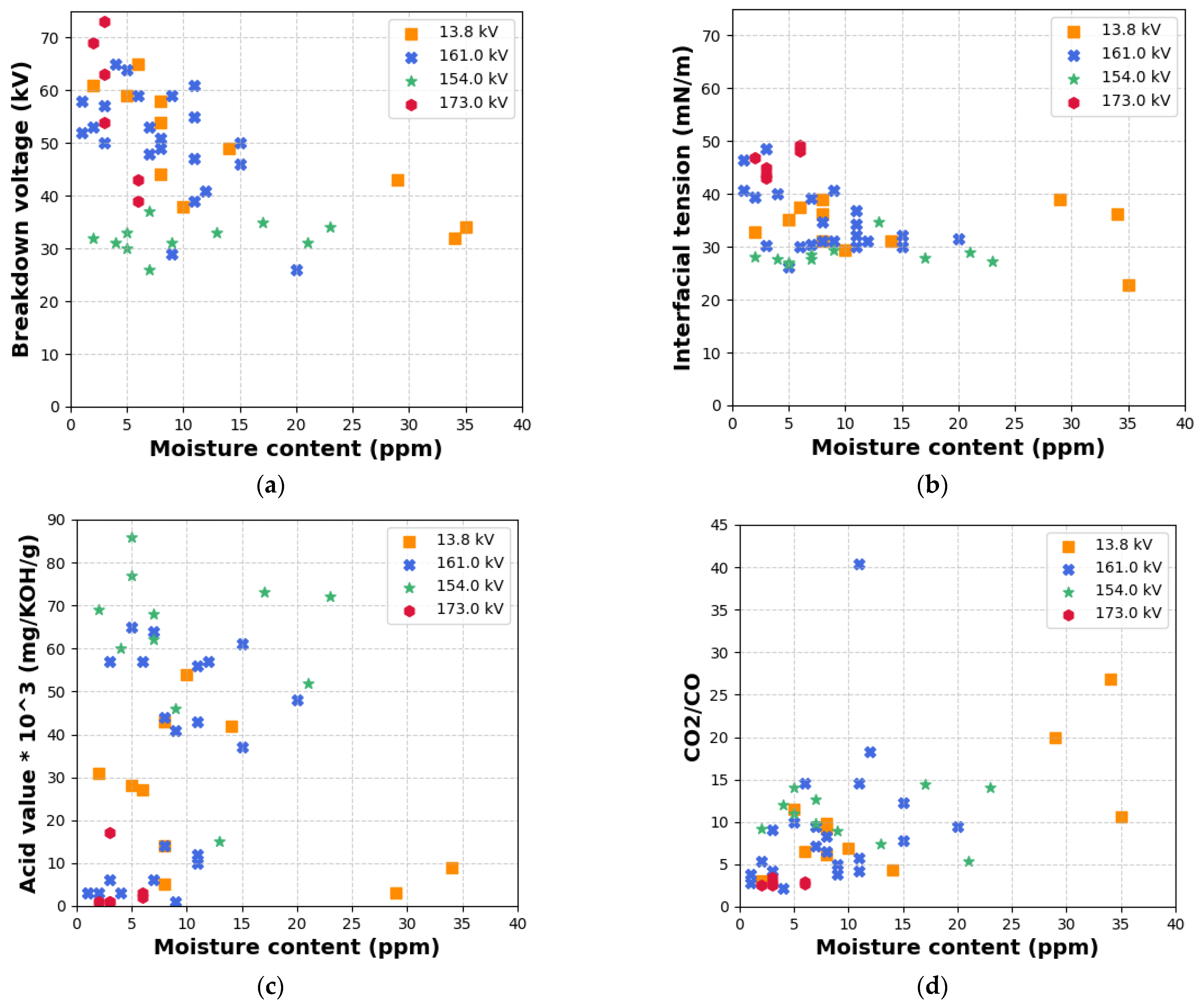
Figure 13a illustrates a consistently negative correlation between moisture content and BDV across all voltage classes. As moisture content increases, BDV values decrease correspondingly. This finding is consistent with the literature, which attributes dielectric strength deterioration to microbubble formation and explains that enhanced ionization is facilitated by elevated moisture levels under electric field stress [26]. Furthermore, high-voltage units (particularly 154 kV and 161 kV) exhibited greater susceptibility to moisture-induced degradation compared to medium-voltage (13.8 kV) units. In Figure 13b, a distinct inverse relationship between moisture content and IFT is observed. Higher moisture levels are associated with reduced IFT, which confirms the catalytic role of water in initiating hydrolysis and oxidation reactions. These reactions generate polar degradation products, the dissolution of which in the insulating liquid leads to a reduction in IFT. Figure 13c reveals the positive correlation between moisture content and acidity, particularly within the 5–20 ppm moisture range. This indicates that the insulation of liquid acidity is predominantly governed by hydrolysis mechanisms, in which water functions as both a reactant and a catalyst, accelerating acid formation. A weak and scattered negative trend is evident in Figure 13d, where the CO₂/CO ratio marginally decreases with increasing moisture content. This ratio is a known indicator of cellulose insulation degradation. The weak correlation implies that moisture alone does not directly influence this ratio, highlighting the role of other contributory factors such as thermal stress, oxidative degradation, and ageing duration in cellulose pyrolysis. 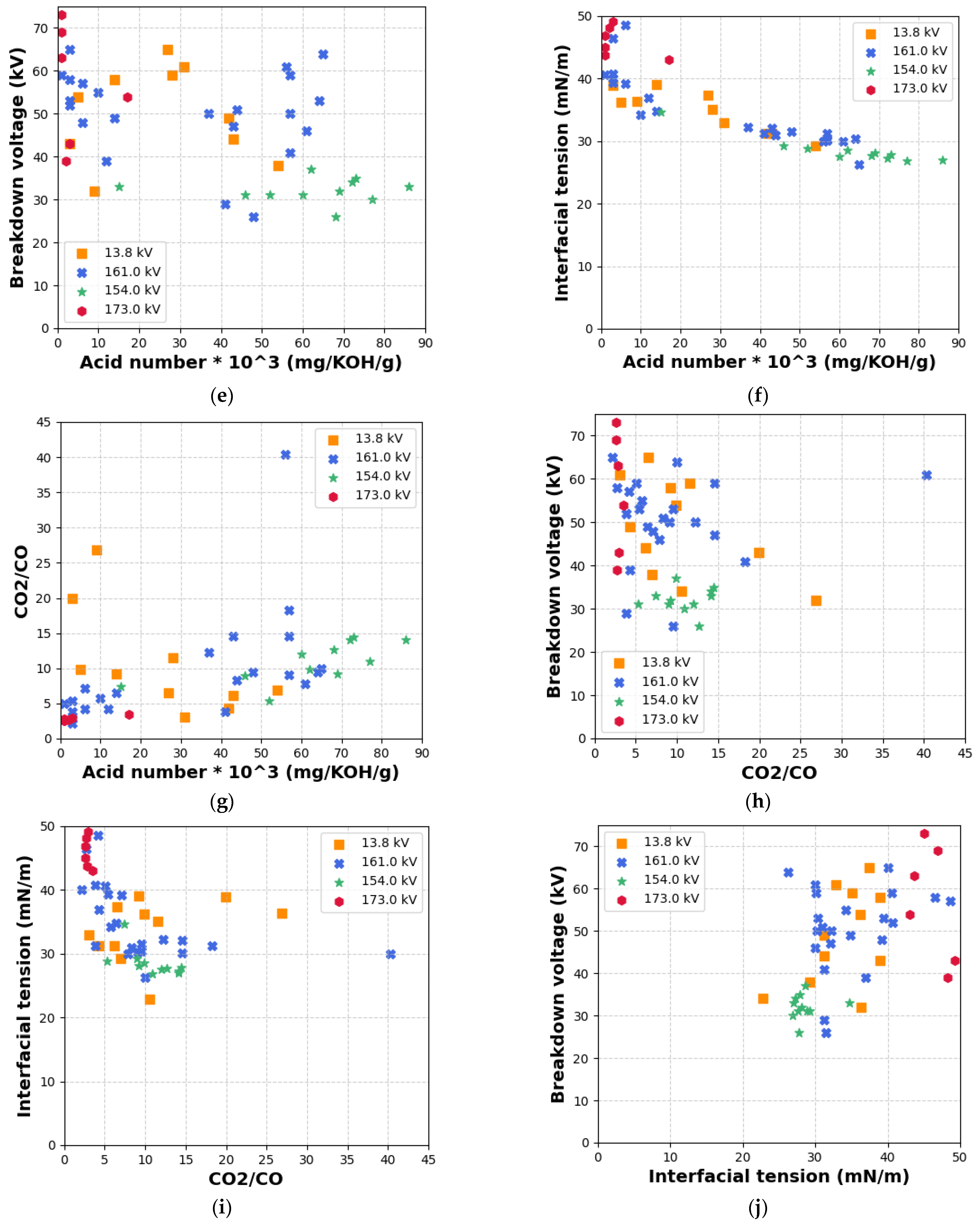As shown in Figure 13e, there is a strong inverse relationship between acid value and BDV, indicating that increased acidity in the insulating fluid serves as a strong marker for declining dielectric strength and impending insulation failure.

Similarly, Figure 13f demonstrates the existence of a negative correlation between acid value and IFT. The reduction in IFT with increasing acid content supports the role of oxidation byproducts, particularly organic acids, in diminishing the surface activity of the insulating liquid. This reinforces the acid value and IFT as coupled indicators for transformer condition assessment. In Figure 13g, a moderate positive correlation is observed between acid value and the CO₂/CO ratio. This relationship suggests that oxidative ageing, as reflected by elevated acid values, often coincides with cellulose decomposition, which releases CO and CO₂ gases [27]. Nonetheless, the scattered distribution of data points indicates that the relationship is not perfectly synchronous, and that parallel degradation processes may also influence gas evolution. Figure 13h presents the weak inverse correlation between BDV and the CO₂/CO ratio, suggesting that while gas ratios provide insight into paper insulation degradation, BDV is more directly affected by moisture and acidity than gas composition alone. In Figure 13i, a negative trend is noted between the CO₂/CO ratio and IFT, implying that increased gas evolution due to cellulose ageing corresponds to a decline in IFT. This observation further supports the coupling of gas evolution indicators with surface-active degradation parameters [28,29]. Finally, Figure 13j shows the strong positive relationship between IFT and BDV, where higher IFT values align with higher BDV values. This correlation confirms that reduced IFT is indicative of surface-active contaminants in the insulating fluid, which impair dielectric performance.

Furthermore, the comprehensive integration of transformer fault classification schemes employed in this study, emphasizing key physicochemical and dielectric properties, offers a multi-dimensional perspective on insulation health. Evaluation using an RF classifier underscores both congruence and divergence among diagnostic outcomes. Notably, 90% of the units satisfied the BDV threshold, and 98% fell within acceptable moisture content limits, indicating robust dielectric strength and moisture control in the majority of units. However, IFT emerged as a critical indicator of insulating liquid degradation, with only 26% of units maintaining values above the standard 40 mN/m benchmark. In addition, this chemical degradation is corroborated by the high incidence of thermal faults predicted by the RF classifier under the CIGRÉ diagnostic scheme, which classified 93.18% of the transformers as thermally stressed. In comparison, RRM and IRM identified thermal faults in 28.6% and 27.9% of units, respectively, offering more stratified fault gradation. While DRM categorized 66.67% of units as normal and 33.33% as thermally decomposed, its classification components lack the granularity necessary for nuanced diagnostic interpretation. Conversely, the tiered temperature-based classification in RRM and IRM provided enhanced alignment with the physicochemical deterioration observed, notably in terms of IFT and acid value. Further substantiating these insights is the CO₂/CO ratio, a proxy for paper degradation severity. Only 58% of the samples exhibited values within the recommended range of 3–10, implying a combination of early-stage and long-term cellulose deterioration across the units. The elevated CO₂/CO ratios observed in a subset of units are consistent with the thermal stress signals flagged by the CIGRÉ method, reinforcing its diagnostic sensitivity. Collectively, these results suggest that although the dielectric strength of most transformers remains functionally stable, there are pervasive chemical indicators of incipient or latent thermal degradation. The complementary roles of advanced classification schemes and physicochemical markers provide critical early-warning capabilities. In particular, CIGRÉ’s aggressive fault detection profile mirrors the widespread suboptimal IFT results, highlighting its utility in proactive insulation health monitoring.

In general, the results across all 13 figures demonstrate that moisture content exhibits a strong inverse relationship with both BDV and IFT, with this degradation trend being most pronounced in the 173 kV and 161 kV transformers. In these higher-voltage units, moisture levels exceeding 15 ppm consistently correspond to a marked decrease in BDV and IFT. Although a similar downward trend is observed in the 138 kV and 154 kV transformers, the decline in BDV and IFT with increasing moisture content is comparatively less severe, reflecting greater insulation stability at a lower voltage stress. As moisture content increases, both the acid number and the CO₂/CO ratio increase across all voltage levels, with the most elevated values recorded in the 173 kV and 161 kV units, suggesting that both insulating liquid oxidation and cellulose degradation are accelerated under high-voltage operating conditions. The relationship between acid number and BDV reveals a consistent decrease in dielectric strength as acidity increases. This is again more significant in the 173 kV and 161 kV transformers, which confirms that acidic byproducts degrade insulating liquids more rapidly under elevated electrical and thermal stress conditions. Similarly, IFT decreases with the increasing acid number, with the steepest decrease evident in 173 kV systems. A clear positive correlation is also observed between acid number and the CO₂/CO ratio, particularly in the 161 kV and 173 kV units, further supporting the interdependence of chemical ageing processes. As the CO₂/CO ratio increases, both BDV and IFT continue to decrease, with the most severe degradation again seen in the 173 kV transformers. Finally, IFT shows a strong positive correlation with BDV across all voltage classes, though this relationship is especially critical in the 173 kV and 161 kV units, where decreases in IFT are closely aligned with dielectric failure. These results suggest that insulation-ageing mechanisms, driven by moisture ingress, acid formation, and paper decomposition, are highly voltage-dependent, with the 173 kV transformers exhibiting the most advanced stages of deterioration.

6. Conclusions

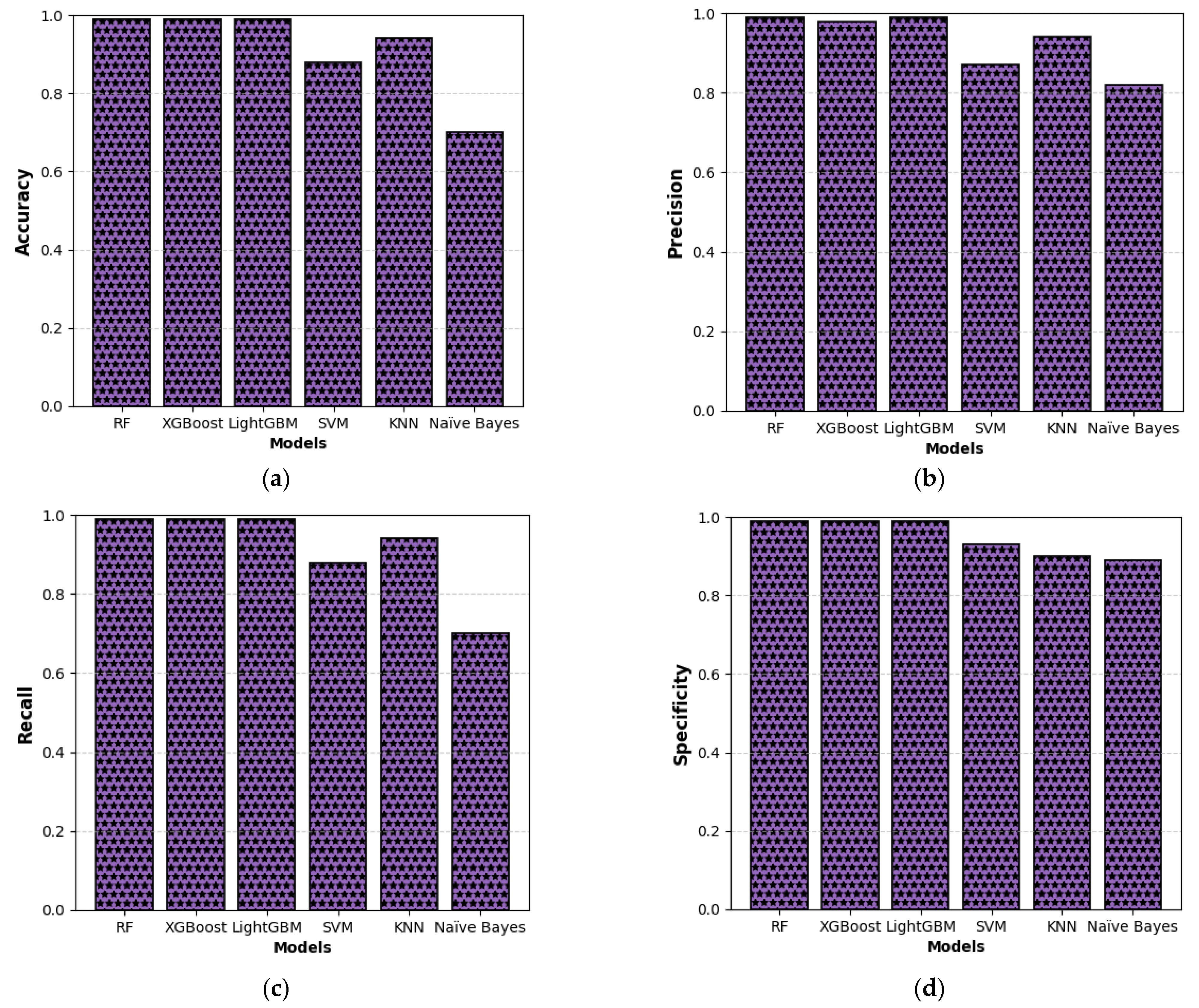
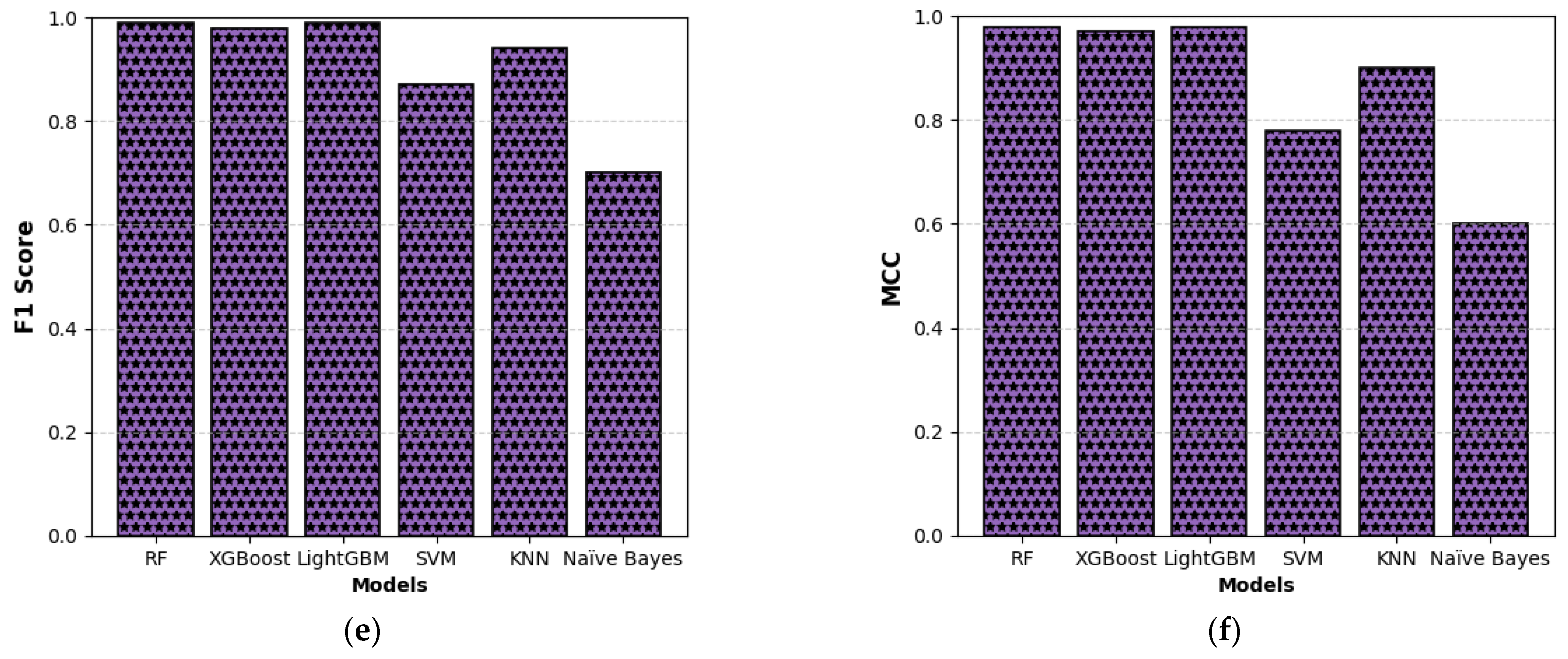
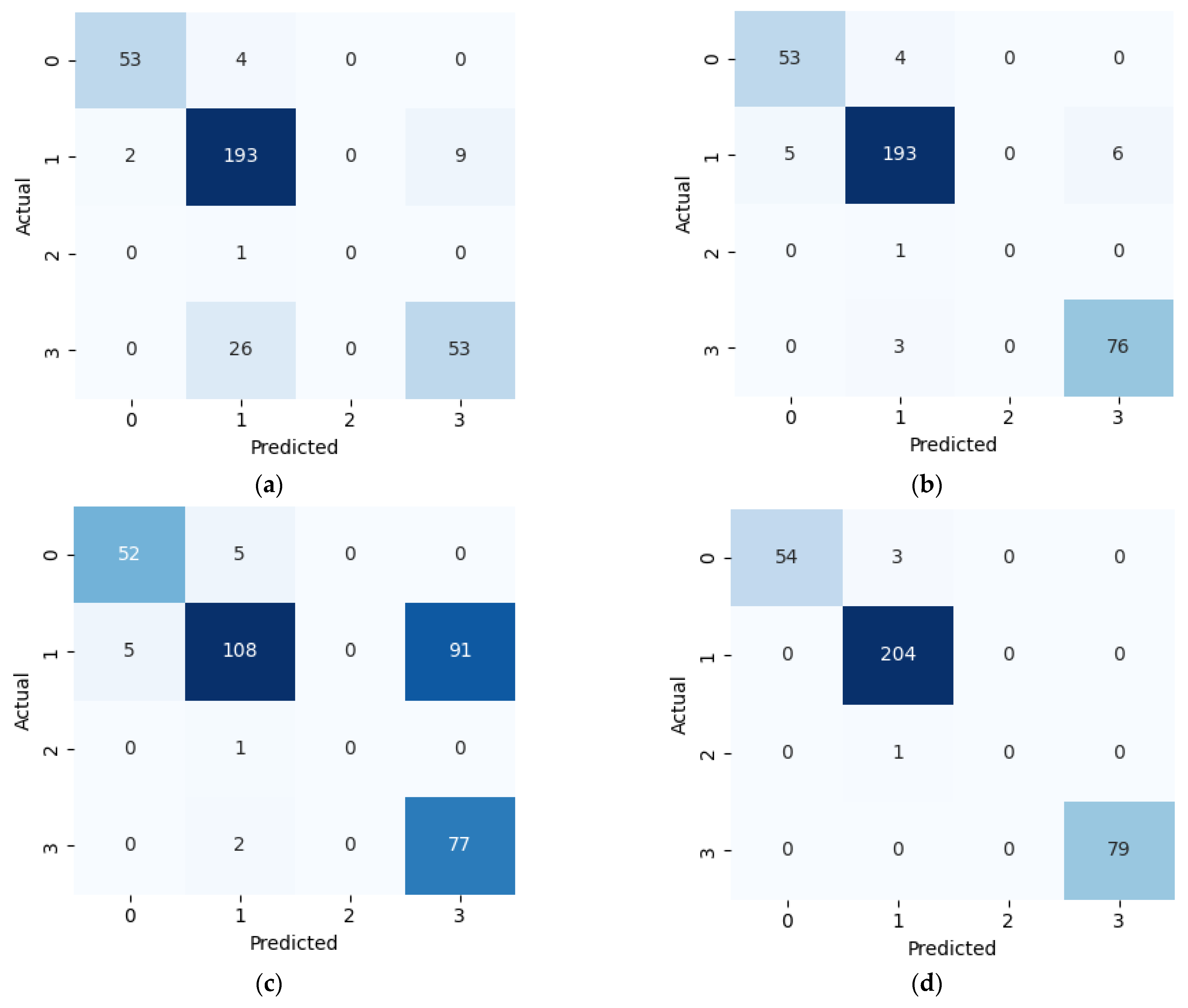
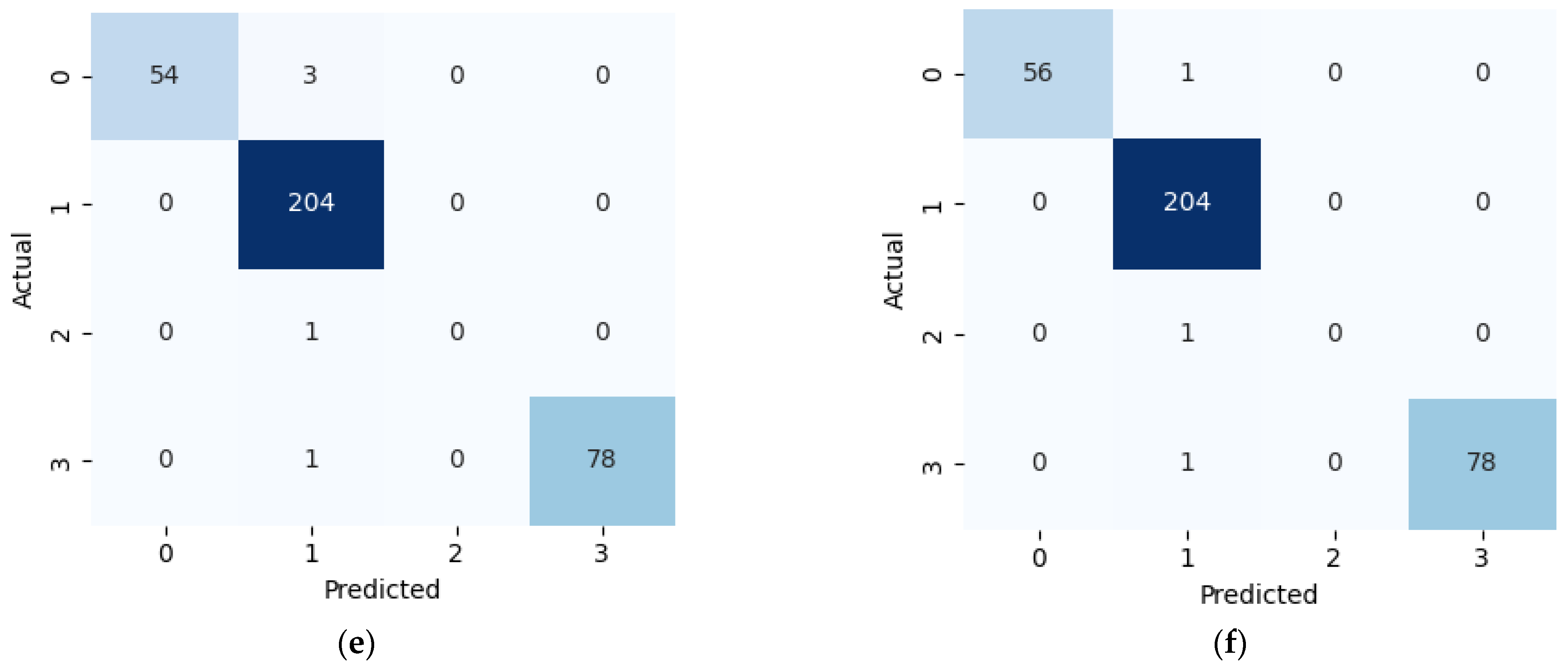
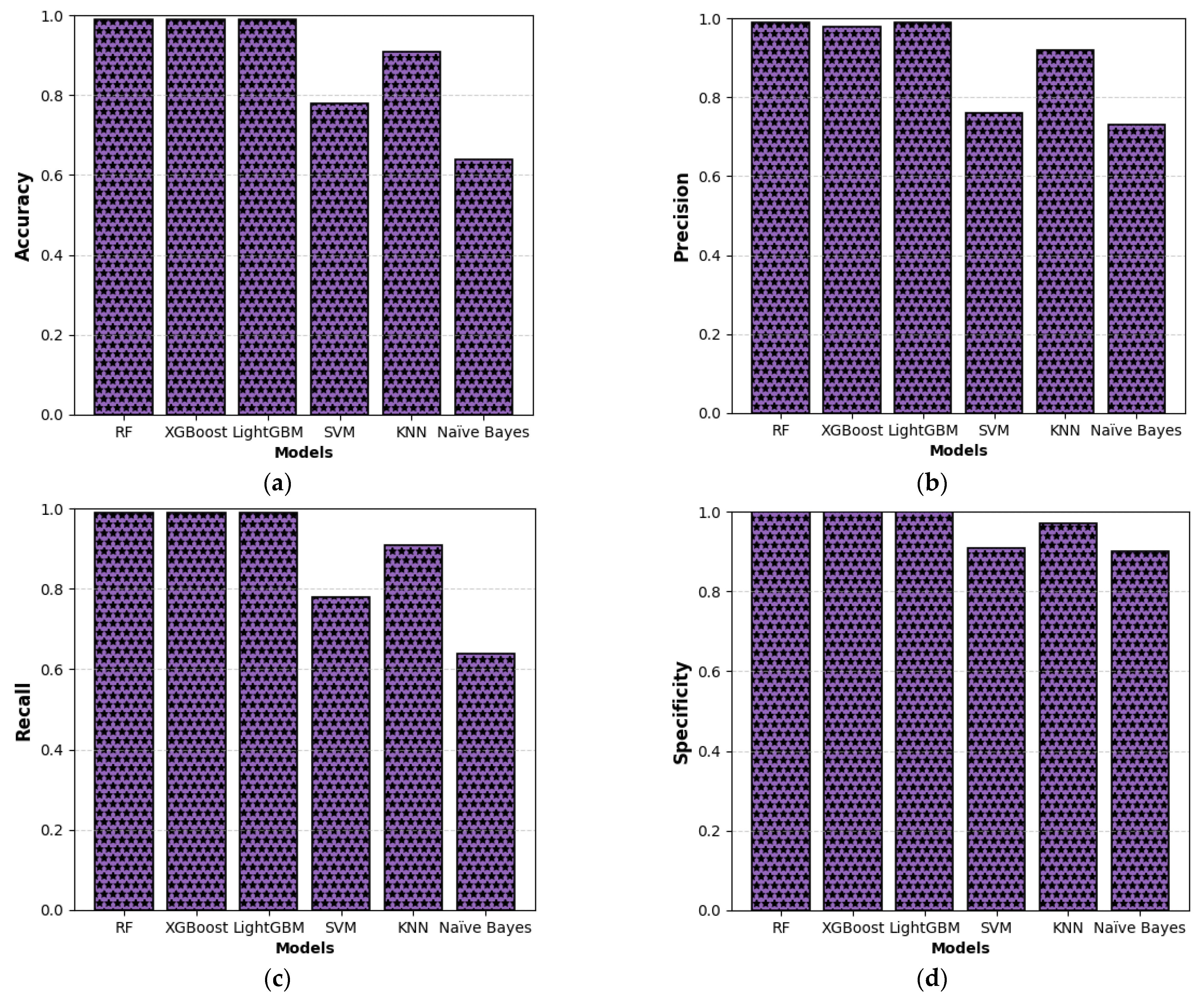
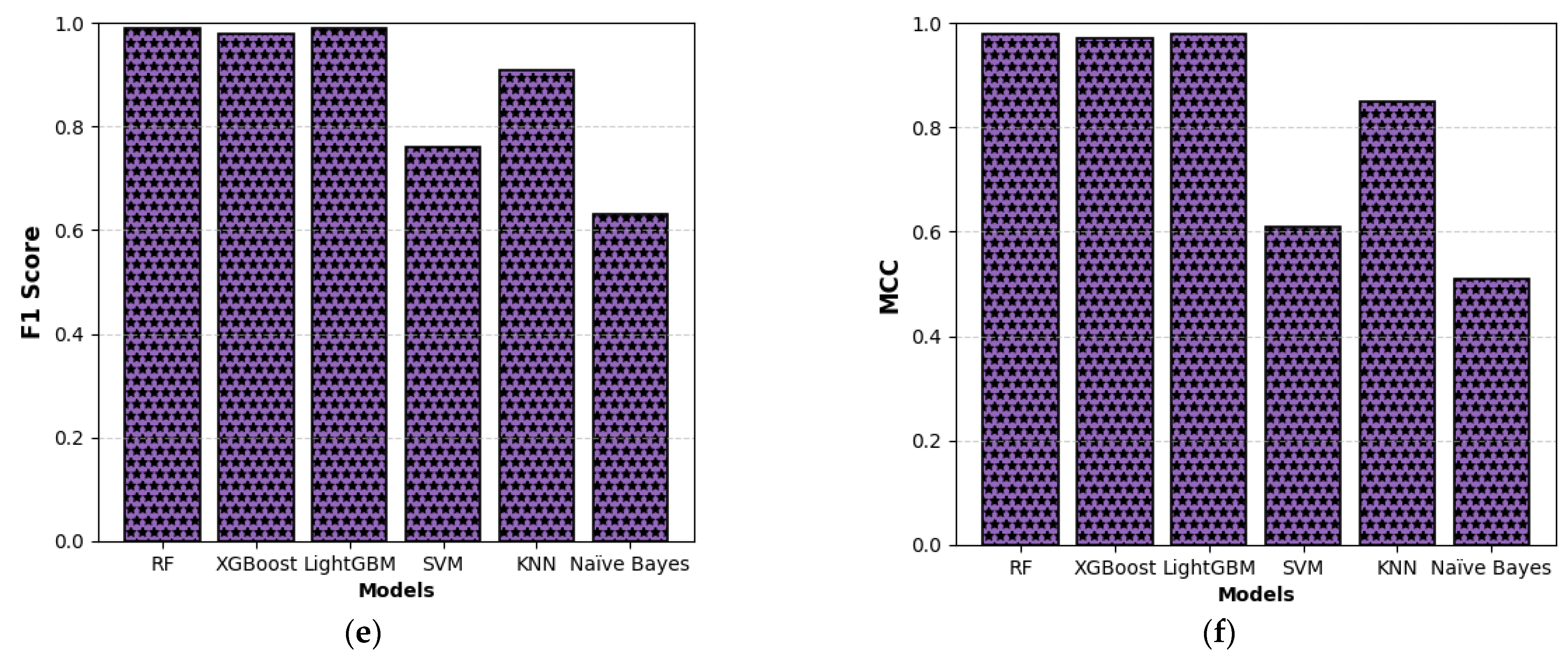
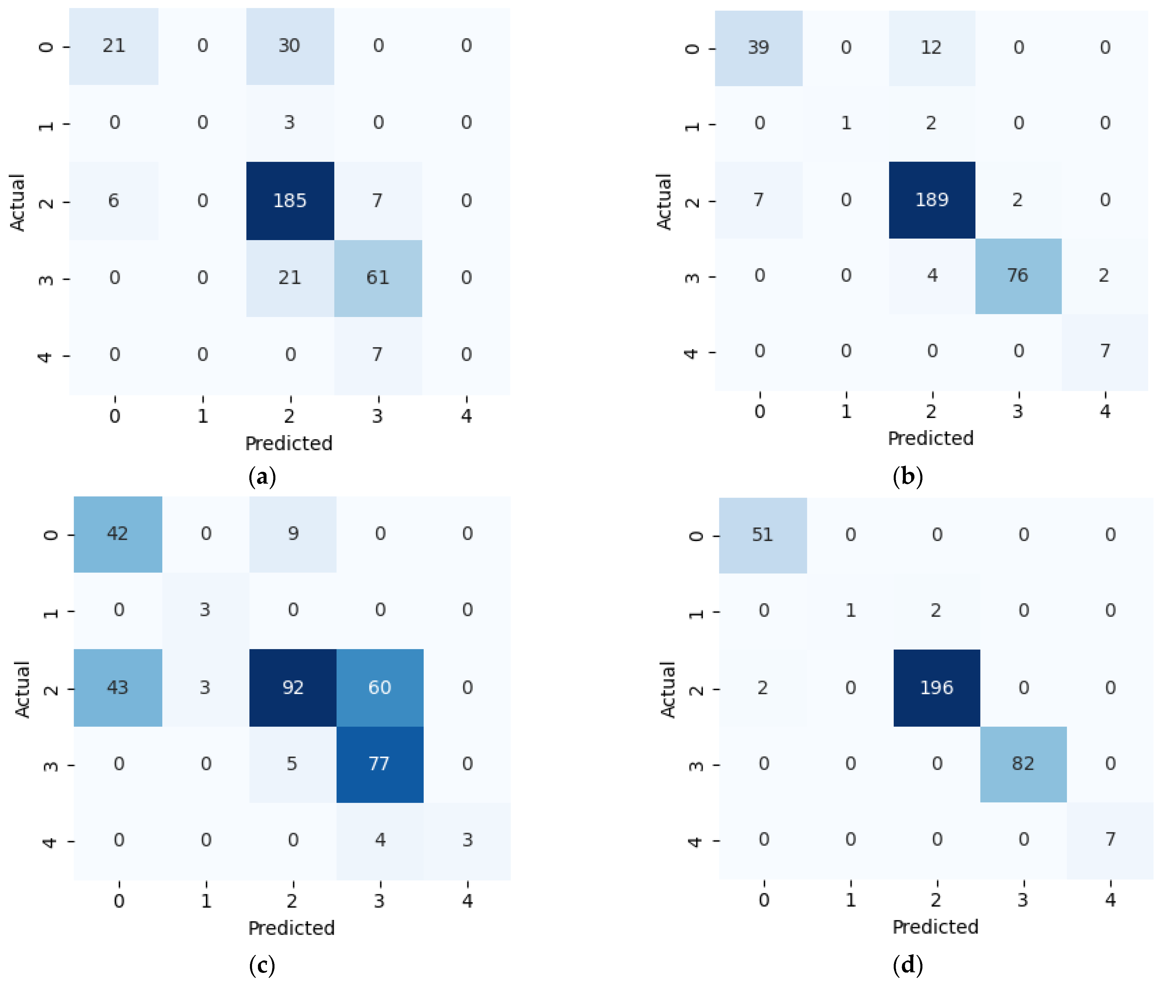
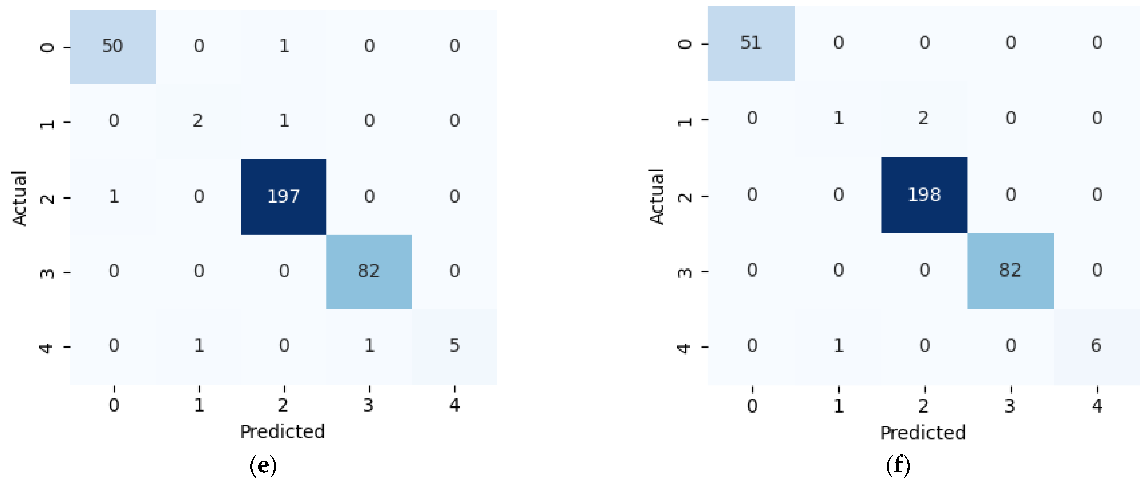
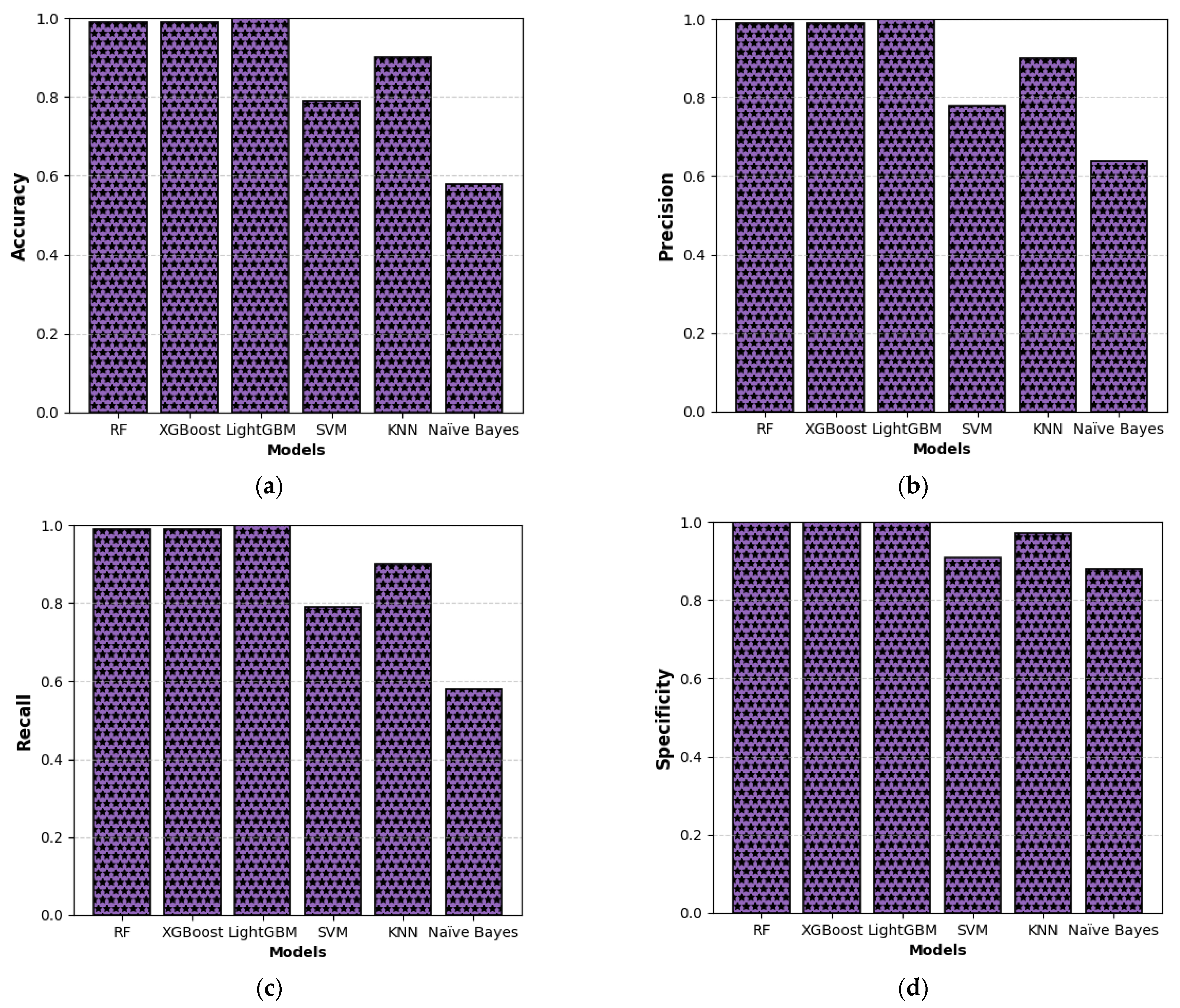
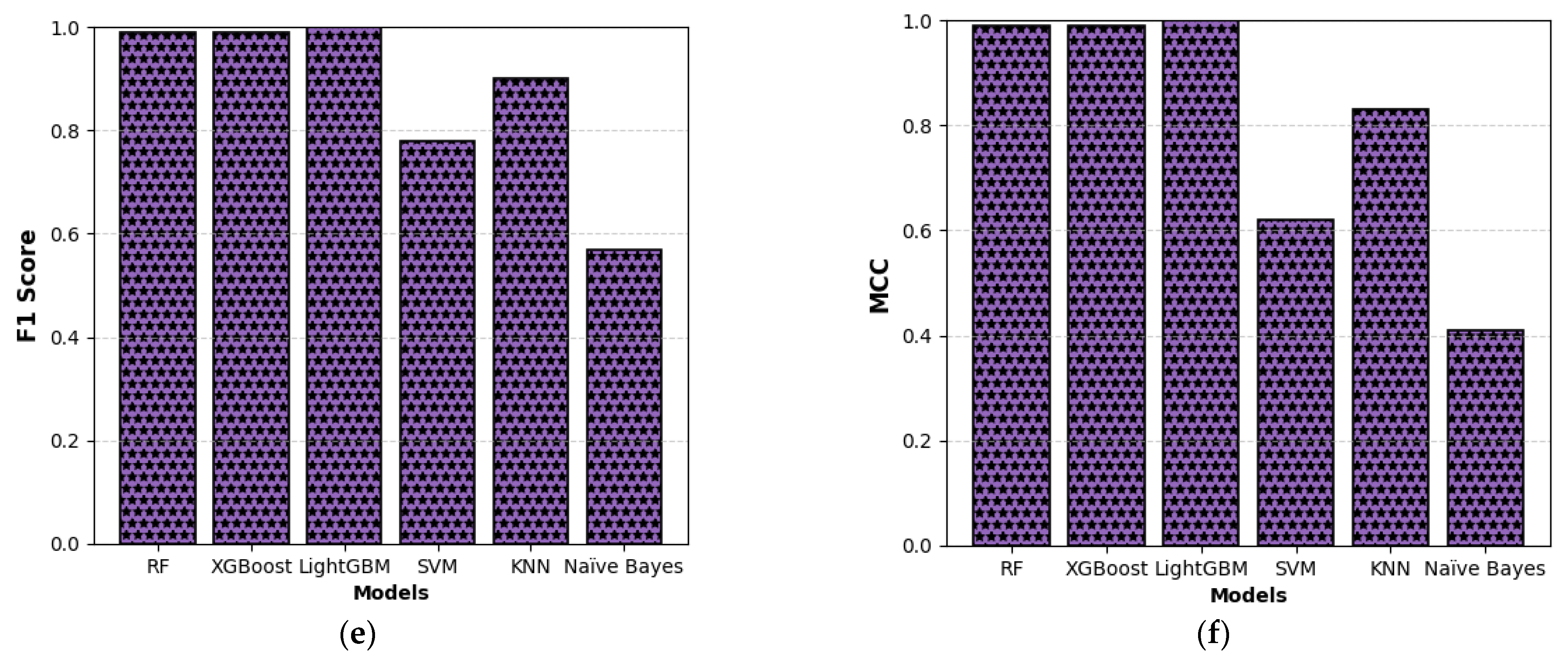
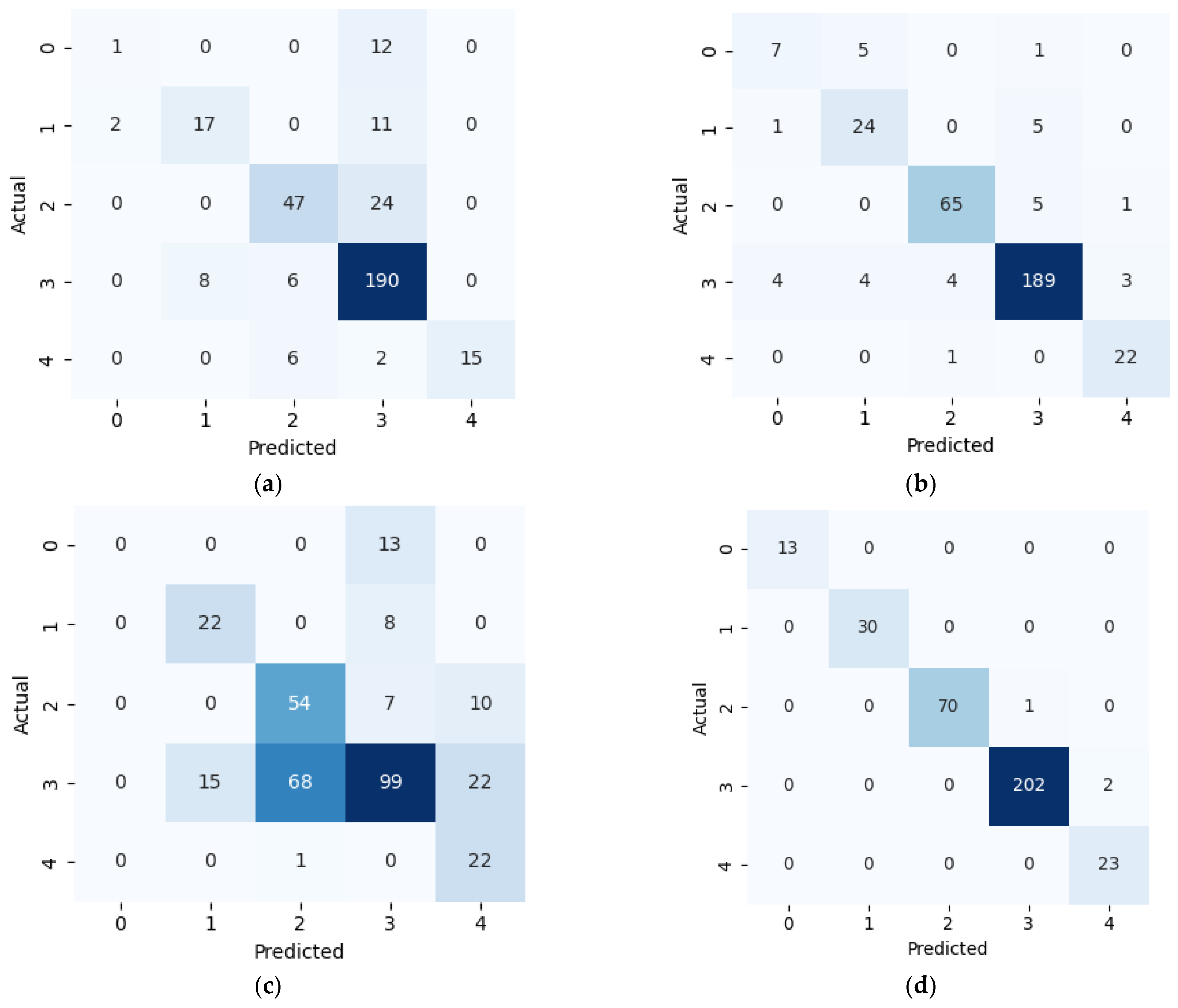
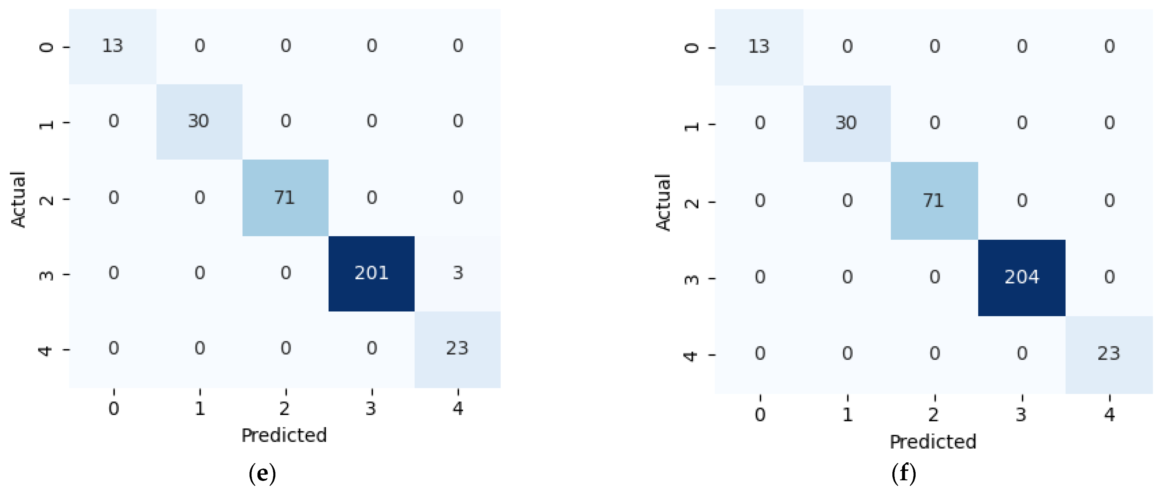
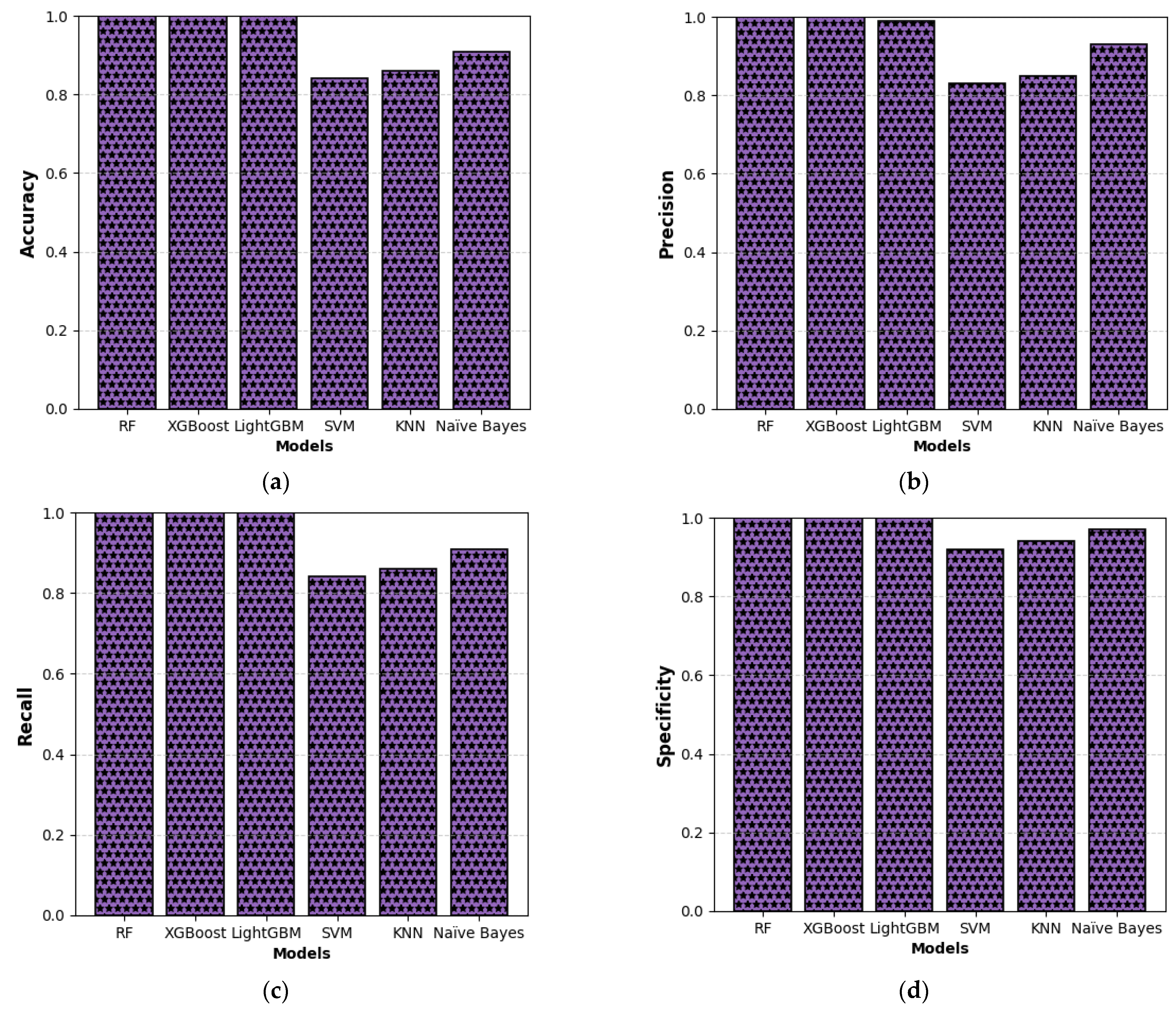
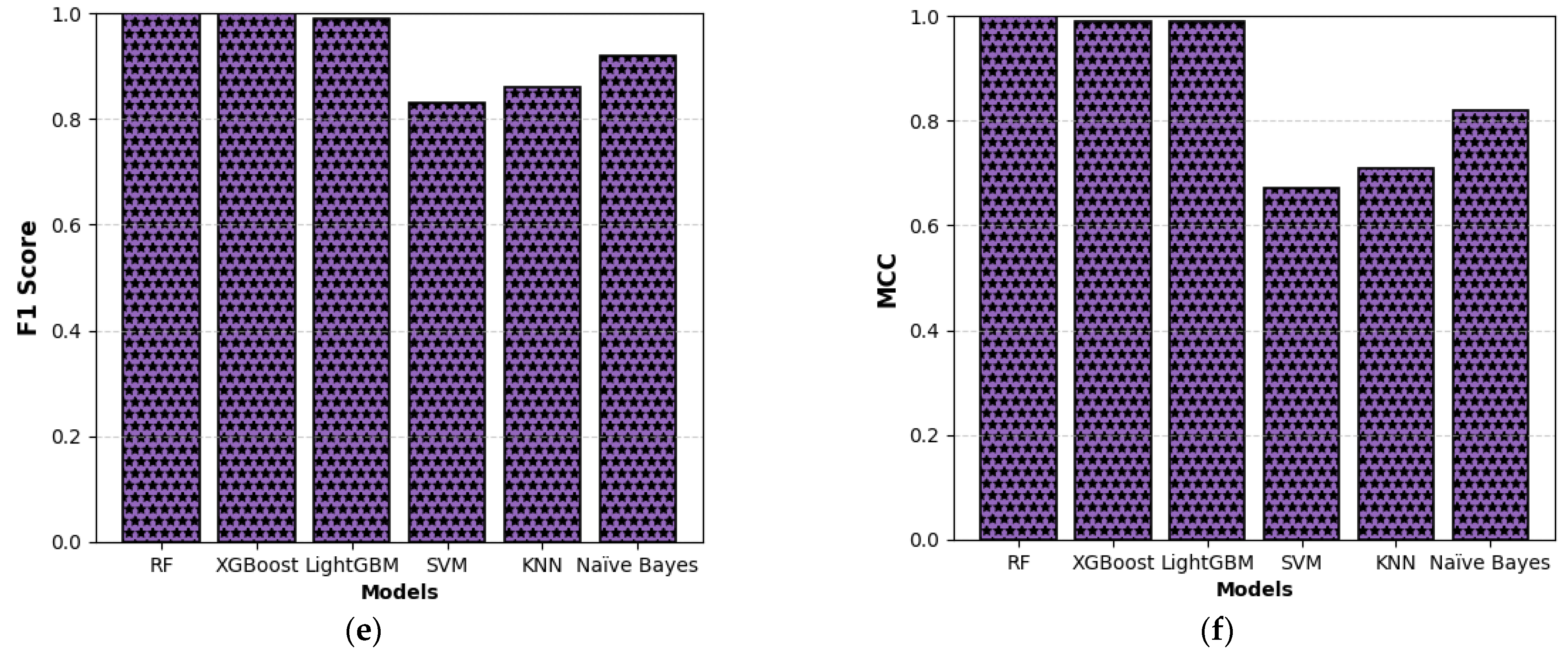
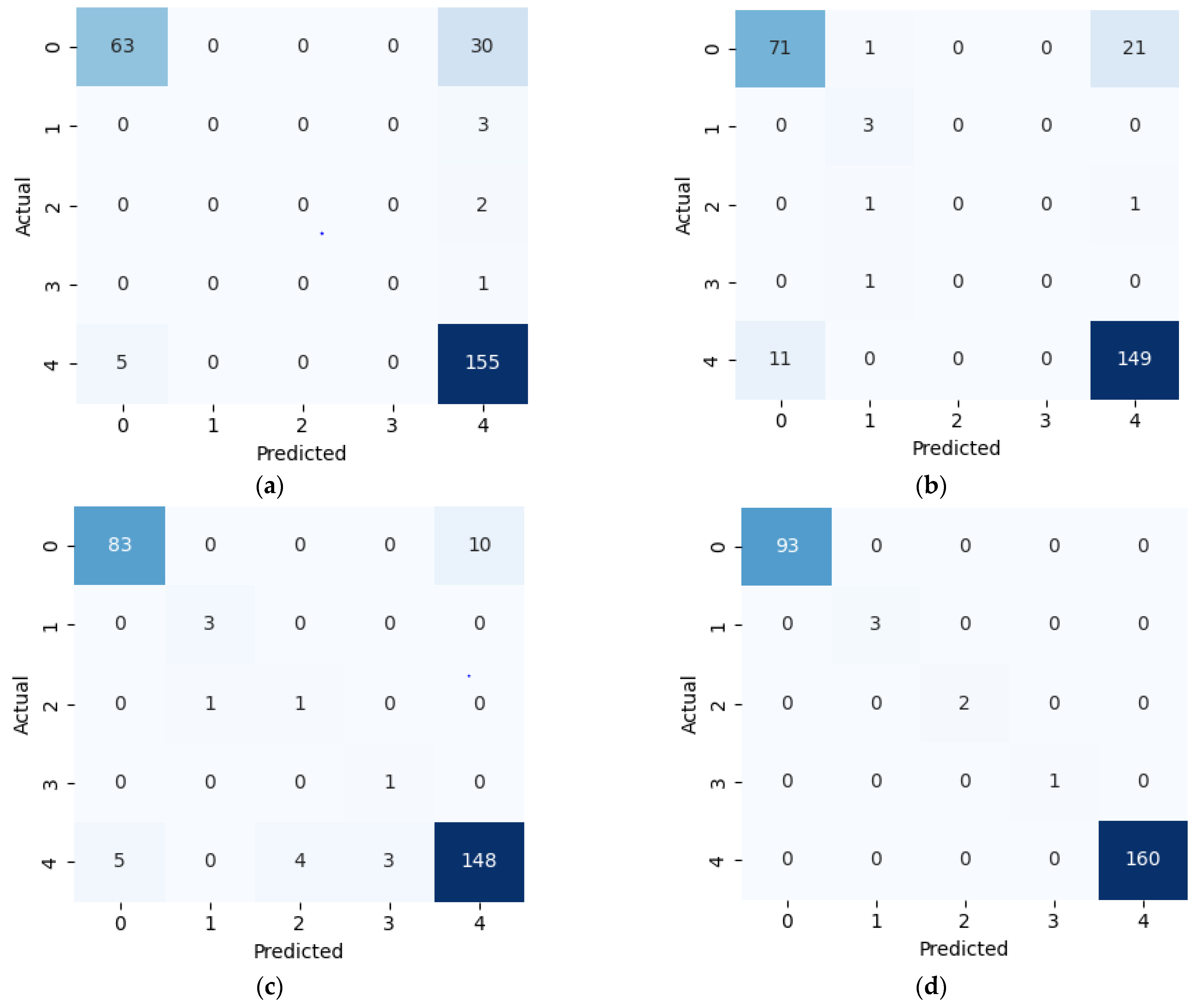
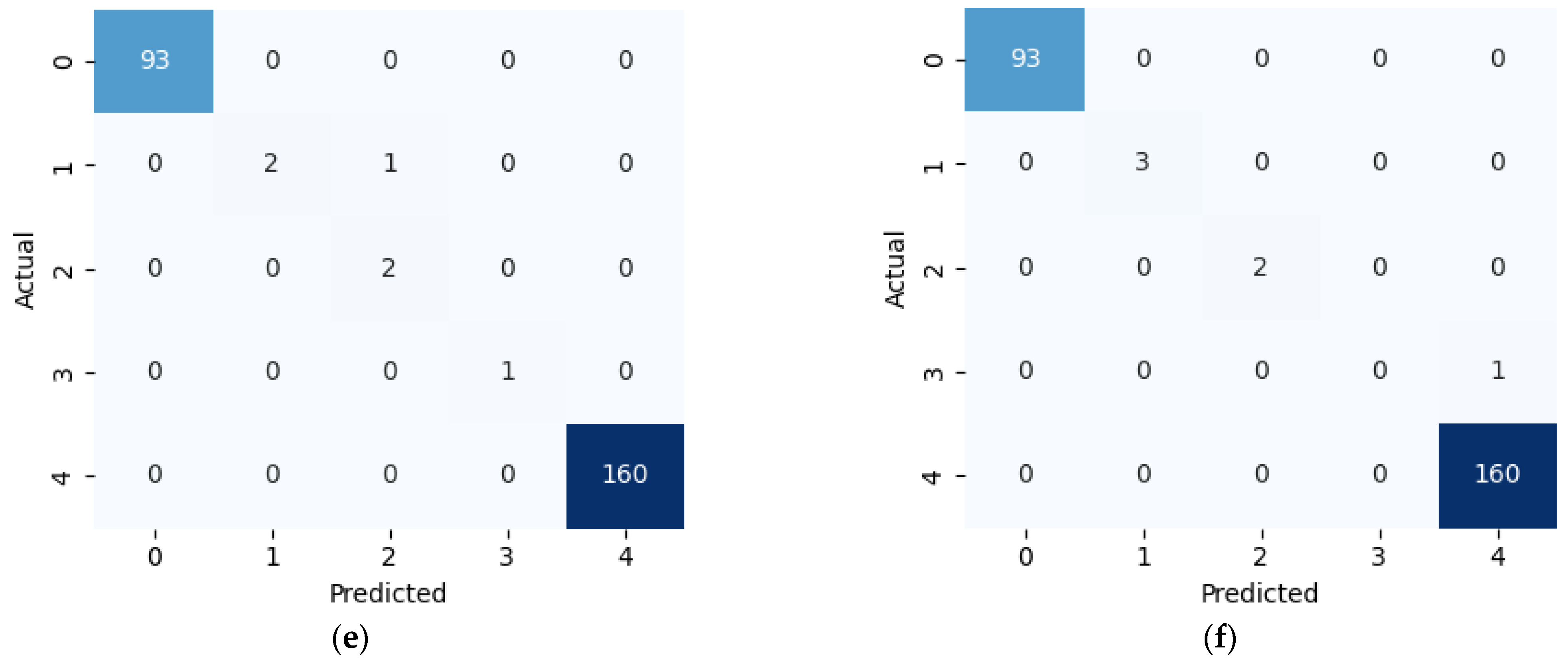
This study presents a comprehensive multiclass classification framework for automated power transformer fault diagnosis using DGA data. Four conventional gas ratio schemes, which are DRM, RRM, IRM, and CIGRÉ, were employed as feature generators, while six supervised ML classifiers were evaluated. The classifiers employed are RF, XGBoost, LightGBM, KNN, SVM, and Naïve Bayes. The results demonstrate that ensemble models, particularly RF and LightGBM, consistently outperform others across all diagnostic schemes. Furthermore, among the non-ensemble models, KNN showed moderate but consistent accuracy, while SVM displayed model instability and degraded performance on fault classes with overlapping features. Naïve Bayes, although weakest under DRM, RRM, and IRM, showed marked improvement under the CIGRÉ diagnostic scheme, suggesting its potential when fault classes are well-separated. The extensive confusion matrix analysis confirmed the high classification reliability of ensemble models, with RF and LightGBM achieving near-perfect diagonal dominance. The findings suggest that ensemble models are the best suited for multiclass DGA-based transformer fault classification. Their ability to generalize well across different diagnostic techniques and maintain high predictive performance under class imbalances makes them ideal for real-world deployment. The study underscores the importance of grid search optimization and 10-fold cross-validation in building reliable fault diagnosis models. In addition, the analysis conducted on the 50 in-service transformers underscores the interconnected degradation mechanisms affecting transformer insulation systems and reinforces the importance of multi-parameter condition monitoring for accurate fault diagnosis and predictive maintenance strategies. Generally, moisture content and acid value emerge as the dominant factors accelerating the degradation of insulating liquids, exerting a direct and measurable influence on both IFT and BDV. Among all the parameters analysed, IFT demonstrates the most consistent and robust correlation with key degradation indicators, positioning it as a reliable standalone diagnostic parameter. In contrast, while the CO₂/CO ratio is a widely recognized marker for assessing paper insulation ageing, its weaker correlation with liquid-phase parameters suggests it should be interpreted in combination with other indicators to provide a comprehensive ageing assessment for insulating liquid. Notably, when data is grouped by voltage class, transformers rated at 13.8 kV exhibit greater variability in measured values. This dispersion reflects less rigorous operational control compared to higher-voltage units, which underscores the need for targeted monitoring strategies in distribution-class assets.

In future studies, the diagnostic framework developed in this work will be applied to real-time, autonomous fault detection by integrating ML models with Internet of Things (IoT) platforms and digital twin technologies. This future direction is expected to significantly enhance transformer health monitoring by enabling continuous data acquisition and intelligent analysis of DGA inputs through embedded sensor networks. Lightweight and scalable ML models will be adapted for deployment on resource-constrained hardware platforms such as ARM Cortex-M microcontrollers, Raspberry Pi, and NVIDIA Jetson Nano. These implementations will aim to support predictive maintenance and early fault identification at the edge. To facilitate this, further research will investigate optimization techniques such as model pruning, quantization, and conversion to formats like TensorFlow Lite or ONNX (open neural network exchange) to reduce memory and processing overhead. Real-time deployment will also require the development of low-latency data pipelines and the adoption of industrial communication protocols such as Modbus, message queuing telemetry transport (MQTT), and controller area network (CAN), which will be explored to ensure seamless integration with supervisory control and data acquisition (SCADA) systems and centralized condition monitoring dashboards. Moreover, future work will explore the creation of a digital twin for power transformers, a dynamic virtual model that mirrors the physical asset by integrating real-time sensor data, historical DGA trends, and ML-driven diagnostic outputs. This digital twin will be used to provide continuous health assessment, predict degradation trajectories, simulate fault scenarios, and inform maintenance decision-making. Such an approach will mark a significant step toward the realization of intelligent, self-monitoring transformer systems within modern smart grid infrastructure.

References

1. Dladla, V.M.; Thango, B.A. Fault Classification in Power Transformers via Dissolved Gas Analysis and Machine Learning Algorithms: A Systematic Literature Review. Appl. Sci. 2025, 15, 2395. [Google Scholar] [CrossRef]
2. Ngwenyama, M.; Gitau, M. Discernment of transformer oil stray gassing anomalies using machine learning classification techniques. Sci. Rep. 2024, 14, 376. [Google Scholar] [CrossRef]
3. Odongo, G.; Musabe, R.; Hanyurwimfura, D. A multinomial DGA classifier for incipient fault detection in oil-impregnated power transformers. Algorithms 2021, 14, 128. [Google Scholar] [CrossRef]
4. Adekunle, A.A.; Oparanti, S.O.; Fofana, I. Performance assessment of cellulose paper impregnated in nanofluid for power transformer insulation application: A review. Energies 2023, 16, 2002. [Google Scholar] [CrossRef]
5. Rao, U.M.; Fofana, I.; Rajesh, K.; Picher, P. Identification and application of machine learning algorithms for transformer dissolved gas analysis. IEEE Trans. Dielectr. Electr. Insul. 2021, 28, 1828–1835. [Google Scholar] [CrossRef]
6. Raghuraman, R.; Darvishi, A. Detecting Transformer Fault Types from Dissolved Gas Analysis Data Using Machine Learning Techniques. In Proceedings of the 2022 IEEE 15th Dallas Circuit and System Conference (DCAS), Dallas, TX, USA, 17–19 June 2022; Institute of Electrical and Electronics Engineers: Piscataway, NJ, USA, 2022; pp. 1–5. [Google Scholar]
7. Benmahamed, Y.; Teguar, M.; Boubakeur, A. Application of SVM and KNN to Duval Pentagon 1 for transformer oil diagnosis. IEEE Trans. Dielectr. Electr. Insul. 2017, 24, 3443–3451. [Google Scholar] [CrossRef]
8. Prasojo, R.A.; Gumilang, H.; Suwarno; Maulidevi, N.U.; Soedjarno, B.A. A fuzzy logic model for power transformer faults’ severity determination based on gas level, gas rate, and dissolved gas analysis interpretation. Energies 2020, 13, 1009. [Google Scholar] [CrossRef]
9. Benmahamed, Y.; Kherif, O.; Teguar, M.; Boubakeur, A.; Ghoneim, S.S. Accuracy improvement of transformer faults diagnostic based on DGA data using SVM-BA classifier. Energies 2021, 14, 2970. [Google Scholar] [CrossRef]
10. Nanfak, A.; Samuel, E.; Fofana, I.; Meghnefi, F.; Ngaleu, M.G.; Hubert Kom, C. Traditional fault diagnosis methods for mineral oil-immersed power transformer based on dissolved gas analysis: Past, present and future. IET Nanodielectrics 2024, 7, 97–130. [Google Scholar] [CrossRef]
11. Sutikno, H.; Prasojo, R.A.; Abu-Siada, A. Machine learning based multi-method interpretation to enhance dissolved gas analysis for power transformer fault diagnosis. Heliyon 2024, 10, e25975. [Google Scholar]
12. Ali, M.S.; Omar, A.; Jaafar, A.S.A.; Mohamed, S.H. Conventional methods of dissolved gas analysis using oil-immersed power transformer for fault diagnosis: A review. Electr. Power Syst. Res. 2022, 216, 109064. [Google Scholar] [CrossRef]
13. Grinsztajn, L.; Oyallon, E.; Varoquaux, G. Why do tree-based models still outperform deep learning on typical tabular data? Adv. Neural Inf. Process. Syst. 2022, 35, 507–520. [Google Scholar]
14. Malakouti, S.M.; Ghiasi, A.R.; Ghavifekr, A.A. AERO2022-flying danger reduction for quadcopters by using machine learning to estimate current, voltage, and flight area. e-Prime-Adv. Electr. Eng. Electron. Energy 2022, 2, 100084. [Google Scholar] [CrossRef]
15. Adekunle, A.A.; Fofana, I.; Picher, P.; Rodriguez-Celis, E.M.; Arroyo-Fernandez, O.H. Analyzing transformer insulation paper prognostics and health management: A modeling framework perspective. IEEE Access 2024, 12, 58349–58377. [Google Scholar] [CrossRef]
16. Ghoneim, S.S.; Baz, M.; Alzaed, A.; Zewdie, Y.T. Predicting the insulating paper state of the power transformer based on XGBoost/LightGBM models. Sci. Rep. 2025, 15, 17836. [Google Scholar] [CrossRef]
17. Seyyedattar, M.; Afshar, M.; Zendehboudi, S.; Butt, S. Advanced EOR screening methodology based on LightGBM and random forest: A classification problem with imbalanced data. Can. J. Chem. Eng. 2025, 103, 846–867. [Google Scholar] [CrossRef]
18. Muslim, M.A. Support vector machine (svm) optimization using grid search and unigram to improve e-commerce review accuracy. J. Soft Comput. Explor. 2020, 1, 8–15. [Google Scholar]
19. Awad, M.; Khanna, R. Support vector machines for classification. In Efficient Learning Machines: Theories, Concepts, and Applications for Engineers and System Designers; Springer: Berlin/Heidelberg, Germany, 2015; pp. 39–66. [Google Scholar]
20. Abdalredha, A.; Sobbouhi, A.; Vahedi, A. Comprehensive flexible framework for using multi-machine learning methods to optimal dynamic transient stability prediction by considering prediction accuracy and time. Results Eng. 2025, 26, 104728. [Google Scholar] [CrossRef]
21. Fuadah, Y.N.; Pramudito, M.A.; Lim, K.M. An optimal approach for heart sound classification using grid search in hyperparameter optimization of machine learning. Bioengineering 2022, 10, 45. [Google Scholar] [CrossRef]
22. Shaban, W.M.; Rabie, A.H.; Saleh, A.I.; Abo-Elsoud, M. Accurate detection of COVID-19 patients based on distance biased Naïve Bayes (DBNB) classification strategy. Pattern Recognit. 2021, 119, 108110. [Google Scholar] [CrossRef]
23. Malakouti, S.M. Estimating the output power and wind speed with ML methods: A case study in Texas. Case Stud. Chem. Environ. Eng. 2023, 7, 100324. [Google Scholar] [CrossRef]
24. Hussain, S.; Raza, Z.; Giacomini, G.; Goswami, N. Support vector machine-based classification of vasovagal syncope using head-up tilt test. Biology 2021, 10, 1029. [Google Scholar] [CrossRef] [PubMed]
25. Jiang, X.; Wang, J.; Meng, Q.; Saada, M.; Cai, H. An adaptive multi-class imbalanced classification framework based on ensemble methods and deep network. Neural Comput. Appl. 2023, 35, 11141–11159. [Google Scholar] [CrossRef]
26. Yang, C.; Zhao, T.; Liu, Y.; Yang, J.; Xu, J.; Xu, Y. Effect of electric field on bubble generation and dissolution characteristics in oil–paper insulation. High Volt. 2025, 10, 480–492. [Google Scholar] [CrossRef]
27. Adekunle, A.A.; Oparanti, S.O.; Fofana, I.; Picher, P.; Rodriguez-Celis, E.M.; Arroyo-Fernandez, O.H.; Meghnefi, F. Degradation Mechanisms of Cellulose-Based Transformer Insulation: The Role of Dissolved Gases and Macromolecular Characterisation. Macromol 2025, 5, 20. [Google Scholar] [CrossRef]
28. Gajbhiye, R. Effect of CO2/N2 mixture composition on interfacial tension of crude oil. ACS Omega 2020, 5, 27944–27952. [Google Scholar] [CrossRef]
29. Drexler, S.; Correia, E.L.; Jerdy, A.C.; Cavadas, L.A.; Couto, P. Effect of CO2 on the dynamic and equilibrium interfacial tension between crude oil and formation brine for a deepwater Pre-salt field. J. Pet. Sci. Eng. 2020, 190, 107095. [Google Scholar] [CrossRef]
Figure 1. Flow diagram of DGA classification process.
Energies 18 03535 g001
Figure 2. Parameter optimization flowchart using grid search.
Energies 18 03535 g002
Figure 3. Ten-fold cross-validation.
Energies 18 03535 g003
Figure 4. Confusion matrix for multiclass classification.
Energies 18 03535 g004
Figure 5. (a) Accuracy comparison with classifiers. (b) Precision comparison with classifiers. (c) Recall comparison with classifiers. (d) Specificity comparison with classifiers. (e) F1 score comparison with classifiers. (f) MCC comparison with classifiers.
Energies 18 03535 g005aEnergies 18 03535 g005b
Figure 6. (a) SVM confusion matrix. (b) KNN confusion matrix. (c) Naïve Bayes confusion matrix. (d) Random forest confusion matrix. (e) XGBoost confusion matrix. (f) LightGBM confusion matrix. Here, 0 represents arcing, 1 represents normal, 2 represents partial discharge, and 3 represents thermal decomposition.
Energies 18 03535 g006aEnergies 18 03535 g006b
Figure 7. (a) Accuracy comparison with classifiers. (b) Precision comparison with classifiers. (c) Recall comparison with classifiers. (d) Specificity comparison with classifiers. (e) F1 score comparison with classifiers. (f) MCC comparison with classifiers.
Energies 18 03535 g007aEnergies 18 03535 g007b
Figure 8. (a) SVM confusion matrix. (b) KNN confusion matrix. (c) Naïve Bayes confusion matrix. (d) Random forest confusion matrix. (e) XGBoost confusion matrix. (f) LightGBM confusion matrix. (0 represents high energy discharge-arcing, 1 represents low-temperature thermal fault, 2 represents normal, 3 represents thermal fault-T > 700 °C, 4 represents thermal fault-T < 700 °C).
Energies 18 03535 g008aEnergies 18 03535 g008b
Figure 9. (a) Accuracy comparison with classifiers. (b) Precision comparison with classifiers. (c) Recall comparison with classifiers. (d) Specificity comparison with classifiers. (e) F1 score comparison with classifiers. (f) MCC comparison with classifiers.
Energies 18 03535 g009aEnergies 18 03535 g009b
Figure 10. (a) SVM confusion matrix. (b) KNN confusion matrix. (c) Naïve Bayes confusion matrix. (d) Random forest confusion matrix. (e) XGBoost confusion matrix. (f) LightGBM confusion matrix. Here, 0 represents discharges of high intensity, 1 represents discharges of low intensity, 2 represents thermal defect (>700 °C), 3 represents normal, 4 represents temperature range (300–700 °C).
Energies 18 03535 g010aEnergies 18 03535 g010b
Figure 11. (a) Accuracy comparison with classifiers. (b) Precision comparison with classifiers. (c) Recall comparison with classifiers. (d) Specificity comparison with classifiers. (e) F1 score comparison with classifiers. (f) MCC comparison with classifiers.
Energies 18 03535 g011aEnergies 18 03535 g011b
Figure 12. (a) SVM confusion matrix. (b) KNN confusion matrix. (c) Naïve Bayes confusion matrix. (d) Random forest confusion matrix. (e) XGBoost confusion matrix. (f) LightGBM confusion matrix. (0 represents arcing, 1 represents normal, 2 represents overheating (paper), 3 represents partial discharge, and 4 represents thermal fault).
Energies 18 03535 g012aEnergies 18 03535 g012b
Figure 13. (a) Relationship between moisture and BDV. (b) Relationship between moisture and IFT. (c) Relationship between moisture and ACV. (d) Relationship between moisture and CO2/CO. (e) Relationship between ACV and BDV. (f) Relationship between ACV and IFT. (g) Relationship between ACV and CO2/CO. (h) Relationship between CO2/CO and BDV. (i) Relationship between CO2/CO and IFT. (j) Relationship between IFT and BDV.
Energies 18 03535 g013aEnergies 18 03535 g013b