Abstract
Non-active current in the time domain is considered for application to the diagnostics and classification of loads in power grids based on waveform-distortion characteristics, taking as a working example several recordings of the pantograph current in an AC railway system. Data are processed with a deep autoencoder for feature extraction and then clustered via k-means to allow identification of patterns in the latent space. Clustering enables the evaluation of the relationship between the physical meaning and operation of the system and the distortion phenomena emerging in the waveforms during operation. Euclidean distance (ED) is used to measure the diversity and pertinence of observations within pattern groups and to identify anomalies (abnormal distortion, transients, …). This approach allows the classification of new data by assigning data to clusters based on proximity to centroids. This unsupervised method exploiting non-active current is novel and has proven useful for providing data with labels for later supervised learning performed with the 1D-CNN, which achieved a balanced accuracy of 96.46% under normal conditions. ED and 1D-CNN methods were tested on an additional unlabeled dataset and achieved 89.56% agreement in identifying normal states. Additionally, Grad-CAM, when applied to the 1D-CNN, quantitatively identifies the waveform parts that influence the model predictions, significantly enhancing the interpretability of the classification results. This is particularly useful for obtaining a better understanding of load operation, including anomalies that affect grid stability and energy efficiency. Finally, the method has been also successfully further validated for general applicability with data from a different scenario (charging of electric vehicles). The method can be applied to load identification and classification for non-intrusive load monitoring, with the aim of implementing automatic and unsupervised assessment of load behavior, including transient detection, power-quality issues and improvement in energy efficiency.
1. Introduction
The problem of identifying harmonic sources has been a subject of discussion for a long time, and various approaches have been proposed. Classical approaches used before the advent of neural networks (NN), deep learning (DL) and artificial intelligence (AI) were mostly based on harmonic signatures using active, reactive and distortion power or current quantities [1,2]. Elaborated transforms have been explored as tools to extract all valuable information from raw signals. These include Fourier transform and its short-time version, S-transform [3,4] and its adaptive version [5], wavelet transform (WT) [4,6] and empirical mode decomposition (EMD) [7]. Such methods are particularly attractive when dealing with transient phenomena [5,8,9], although there are approaches that involve feeding such transients directly to the NN [10,11,12]. We emphasize that these approaches have been proposed as tools to classify different power-quality transients [10,11] from a predetermined list; only [12] addresses anomaly detection applied to the railway environment; however, it focuses on transients identified by the Hilbert transform and uses a supervised method, like a 1D-CNN. This demonstrates the novelty of the present approach, which covers anomalies not previously identified and quantified with an unsupervised approach.
Despite the prevalence of a focus on the frequency domain in research produced until the last decade, time-domain (TD) approaches have been also proposed and have become more popular for use in combination with DL [12,13,14].
Non-intrusive load monitoring (NILM) and distortion classification aim at improving the availability, quality and safety of modern grids [15,16,17] but face significant challenges in presence of highly dynamic loads and non-ideal grid response. Whereas pure NILM focuses on energy disaggregation of appliances, the use of distortion classification provides important support for disambiguating typical scenarios involving contemporary switching events, similar V-I patterns, etc. Load monitoring and classification can in general support the following features:
- grid protection and management (including stability) that are applicable at large scales (e.g., in distribution), but also at the small scale of a microgrid, including renewables and highly dynamic or susceptible loads [18,19];
- control of power flow to improve the quality of service, in particular in terms of voltage fluctuations and transients [20];
- power-quality control encompassing both traditional harmonic distortion and disturbance at higher frequency, which are emerging today as possible threats to grid control and metering that directly affect power-line communication protocols [21,22,23,24]; past studies demonstrate that interference with the metering function can occur at various frequency ranges within the harmonic and supraharmonic domains, affecting not only the overall intensity, but also specific parts of the waveform, as in the case of pulsed disturbances [22];
- energy efficiency from a multitude of perspectives:
- −
- identification of energy-wasting devices or, in general, devices with less-than-ideal power profiles [25];
- −
- demand management and load balancing as part of grid control;
- −
- identification of power losses in susceptible grid elements (namely transformers and cables) and in the loads themselves that occur as a consequence of excessive distortion;
- −
- correct accounting for harmonic power losses in the estimation of power absorption and energy efficiency [26];
- fair tariffing and billing, associating variable tariffs with the level of load “virtuosity” as soon as a load is connected to the grid; this includes linking tariffs potentially disruptive events that may cause economic losses and also may incentivize improvements in energy efficiency and reduce associated losses. Conversely, at the user level, usage regulation encourages the use of low-price time slots, a change supported by the use of smart meters [25].
Another interesting application is the monitoring and evaluation of long-term unsupervised power -quality (PQ) measurements as a form of big-data analytics [27]. A previous application involving transient removal from recorded data in power grids is reported in [28].
Even accurate and sophisticated DL methods can suffer from intrinsic variance in input data (this will be addressed in this work by evaluating the effects of noise in input data) and from the presence of new unlabeled data [29,30] (e.g., a new type of load or an unforeseen operating condition).
Focusing on AC railways as a network featuring moving loads (the rolling stock, RS) with variable powering and operating conditions (OCs), this study emphasizes single-point monitoring methods applied at the pantograph interfacing port. While voltage drops can affect voltage values along the contact line (and thus affect the calculated power terms depending on the measurement location in the network), analysis of the pantograph current alone offers an advantage because the pantograph current can be directly related to the line current sourced by the Traction Power Station (TPS), which represents the internal coupling point. In other words, there is a more accurate and direct relationship between the TPS current and the RS pantograph current.
RS, with its absorption peaks during tractioning and intense reverse power flow during braking, represents a challenging load, with highly dynamic behavior and continuously changing feeding line impedance as it moves [31], which cause the voltage-current relationship to change continuously, especially at high frequencies. Complex and varying harmonic patterns occur depending on the variable OCs [32] and are influenced by the TPS distortion and nearby trains [33].
Basic signal-projection and -classification techniques applied to AC railway data were evaluated in [34], exploring the benefits of each method (principal component analysis (PCA) and partial least squares regression (PLSR)), and discussing TD features useful for load monitoring and distortion tracking (average and extreme values, slope, intersections, etc.) [35].
The number of candidate features that can be extracted with “classical” methods is large. AI techniques can offer significant support for synthesizing pools of highly informative features [36]. Such techniques go through suitable projections and data-dimensionality reduction, which are followed by clustering and classification, including identification of anomalies and outliers [27,36]. For example, image-processing techniques may be equally applicable to frequency-domain spectra [36] and TD waveforms, including V-I trajectories [13,32,37,38].
Information available in TD waveforms can be further exploited by focusing on waveform parts that convey the most relevant information. The advantage of TD waveforms lies in their close relation to load operation, which improves comprehensibility and interpretability for the user. The combinations of information extracted from the TD raw data and possible clustering and classification approaches are countless. Modern artificial intelligence methods may help reduce this complexity, providing effective dimensionality reduction on the one hand and profitable identification of informative features on the other hand [39].
This paper abandons the more classical frequency-domain distortion indexes and discusses the following points:
- Non-active current (NAC) provides good classification performance and characterization of waveform distortion (WD).
- Classification of unlabeled highly-dimensional WD data with a two-step method: first, dimension reduction using deep autoencoder (DAE) and clustering for OC characterization, labeling and anomaly detection (AD); second, cluster assignment based on Euclidean distance (ED) for segmentation of new unlabeled data (not clustered or trained); this classification is unsupervised and has diagnostic and interpretative uses.
- Alternatively, cluster categorization can be utilized for labeling the data, allowing supervised DL algorithms to train and perform monitoring tasks, since such methods depend on reliable labeling to perform well after training and validation. For that purpose, a 1-D CNN is employed as a benchmark for supervised DL in classification tasks, highlighting the potential of cluster-based labels.
- Clustering reveals patterns associated with WD characteristics and system dynamics, including anomalies, thus supporting the identification of outliers without the need for a specific prior criterion. This is a point of novelty with respect to the majority of previous studies and is demonstrated also by considering an additional example, specifically, charging of electric vehicles (EVs).
- Assessment of both classification methods using new unseen data from the same system that are not labeled, but are assigned an OC by inspection of data characteristics.
- Identification of informative waveform features to provide added value to the supervised classification, focusing on the 1-D CNN and using gradient-weighted class activation mapping (Grad-CAM).
The objective is not so much the general classification of PQ disturbances in a power grid, but the characterization of load operation and its changes in OCs to allow the identification of different loads and the separation of anomalous cases, as well as of new, previously unseen loads. This work characterizes WD by segmenting the associated mechanisms with OC variations, allowing unsupervised load characterization. ED allows quantifying the consistency of patterns originating from the same load, including applications for diagnostic purposes, such as identifing outliers and anomalous cases.
The overall structure and the main contributions of this work are graphically described in Figure 1.
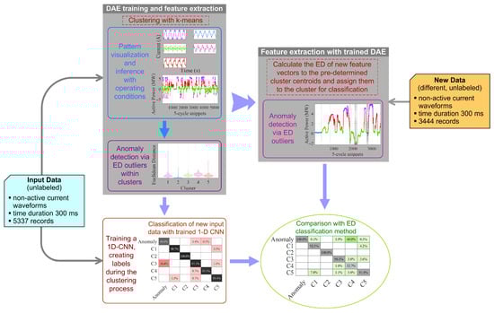
Figure 1.
Overall graphical description of the paper structure and organization.
2. Electric System and Related Power Theory
This section clarifies the approach to NAC extraction and the characteristics of the studied electric system, which will be relevant in the later discussion of clustering and fingerprinting.
2.1. Time-Domain Non-Active Power
Based on Fryze’s theory [40,41], a TD decomposition was applied to the measured waveforms.
Starting from the active current component , the NAC is then the difference between the total current and . The components and are orthogonal, so that they can be summed in quadrature.
where the active power P is directly determined from its TD definition for a sinusoidal signal of period T:
The NAC is calculated as the difference:
2.2. Description of the Electric Power System
Electrified railway systems (ERSs) feature long line branches (with power distribution mostly through overhead conductors) fed by one or more TPSs. In AC railways, traditional TPSs provide power to the line through transformers, whereas more modern converter-based TPSs interface directly and are a cause of increased background distortion. AC railways may work in synchrony with the national grid (at 50 Hz or 60 Hz), or autonomously at Hz (in central Europe), using their own transmission grids [42].
The electrical interactions among the various elements (national and transmission grids, TPSs, overhead lines, return current circuits, signaling systems, RSs, etc.) can be complex. RSs are moving loads that operate dynamically with traction and braking intervals but also include coasting and standstill. Besides converter-based TPSs, they are the other major source of distortion due to a variety of static power-conversion systems that operate onboard (for traction and auxiliary loads) and have emissions overlapping the background distortion [43].
Identification and assessment of RS distortion has the following technical objectives:
- compliance with distortion limits aims at preventing damage to the distribution system and interference with other loads [44];
- distortion limits are also set to limit interference with signaling circuits, such as track circuits [45];
- traction line stability and limitation of overvoltages triggered by RS emissions [46,47].
3. Segmentation and Classification Method
In this work, the DAE is applied to the part of the pantograph current, and this step is followed by clustering. In [32], the DAE was applied to find patterns in WD data of pantograph quantities, showcasing the potential of unsupervised DL and clustering techniques (see Figure 2). While that method effectively characterized WD short-term variations and their relation with OCs, some aspects were not investigated, namely the following:
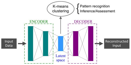
Figure 2.
DAE application to pattern recognition in WD data.
- how to deal with variability or diversity within a cluster and how to use it to verify new unlabeled data;
- the shape and compactness around the clusters’ centroids may be used to identify anomalies and provide information for diagnostic purposes.
This work goes beyond the simple classification task by quantitatively assessing the information conveyed by the various data features, starting the process from the achieved cluster structure in order to provide segmentation of WD data, including AD. This novel approach not only supports robust labeling of data, but also introduces two unique classification methods:
- one method is based on the ED of DAE features and predetermined clusters, evaluating the capacity for transferring segmentation knowledge from the unsupervised learning framework to new unlabeled data;
- the other method uses a more traditional 1-D CNN, ensuring that labeling can be explored with other DL techniques for independent validation.
3.1. DAE and Clustering for Data Segmentation and Labeling
DAE, an unsupervised learning model, is designed to learn a compact input data representation, capturing its significant characteristics and patterns [36]. This enables the model to achieve dimensionality reduction and feature learning. The architecture consists of an encoder, latent space and a decoder.
The choice of DAE over other more traditional methods, such as principal component analysis (PCA), is related to its capacity for modeling complex/complicated non-linear functions with high-dimensional data [48]. While DAE uses non-linear activation functions, PCA is limited to a linear transformation of data and thus has unavoidable limitations.
The encoder, a set of feed-forward filters, transforms the input data into the latent space, where a reduced dimension and a defined number of features represent the data [49]. Simultaneously, the decoder, a set of reverse filters, produces the input reconstruction. By targeting the input and performing back-propagation during training, the model learns the underlying relevant features of the data. The difference between the reconstructed input and the actual input updates the error term, using metrics like mean squared error (MSE) or cosine similarity (CS), in case of highly-dimensional and noisy data.
The encoding step is described by (4):
where the input feature vector u is represented by the coded feature vector z, which propagates through the hidden layers. W are the weights of the network, b is the network biases, and is an activation function.
The decoding step is described by (5), where the coded feature vector z is mapped back to the higher dimension reconstruction y.
Table 1 describes the architecture and the hyper-parameters used in the DAE. The CS is described by (6): it assesses the similarity between two vectors, and , by calculating the cosine of the angle between them, resulting in almost unity values for similar vectors and towards 0 for dissimilar or orthogonal vectors [50].

Table 1.
Autoencoder Architecture and Training Hyper-parameters.
As illustrated in Figure 2, k-means clustering is applied to the latent space representation of the data that are separated based on the WD characteristics extracted by the DAE. The resulting clusters represent the data segmentation and also provide data labeling, conveying information related to the RS OCs and WD.
The k-means clustering algorithm organizes data into a preliminary assigned number of clusters [51]. It measures similarity using ED and employs centroids to represent each cluster [51,52]. Its choice is motivated by its simplicity of interpretation and implementation, together with the capacity for good performance with large datasets, scalability, and suitability for multiple domains [53].
This approach resembles that used in [54] for the classification of PQ transients waveforms, although dimensionality reduction is achieved here with the DAE itself and not by applying PCA at the autoencoder output. The PCA and CS were combined in [54] to associate database labels with the cluster centroids from the observed data. Through this approach, manual analysis of defining the events associated with the clusters is avoided. However, this process requires a dataset with predetermined and reliable labels, and the resultant classification of the clusters is made faster. It is a good alternative for PQ events with such highly distinguishable and separated characteristics, but it is much less effective when only WD characteristics without labels are subject to analysis. Addressing variation of spectral content in the time domain requires that the features captured by the DAE can distinguish unlabeled patterns (not known a priori) with a measurable diagnostic parameter, as proposed in the present work. This process enables the creation of new labels associated with WD features and system characteristics (such as RS type or its OC). The approach in [54] is appropriate when the objective is to identify patterns and segmentation with classification based on one type of event (e.g., voltage variations of different magnitudes, such as dips, swells, interruptions, etc.).
Since the DAE provides data dimensionality reduction, the predetermined number of clusters to be used in k-means is determined using the Calinski–Harabasz criterion [55]. The ED metric used by k-means will be further evaluated for AD.
3.2. Suitability of NAC for Fingerprinting
Good and consistent performance is provided by the active power index (API), which calculates the active power component at each spectrum frequency bin and is able to track the different behaviors of each component for each type of distortion. The use of various non-active power terms has also been discussed in the literature as an indicator for the identification of disturbing loads, both in the frequency domain [56,57] and in the time domain [58,59].
The problem of selecting informative parts of the spectrum for RS classification was investigated in [34], with the following results:
- Active power vs. frequency preserves the sign of power absorption, distinguishing between traction and braking conditions, and has good classification performance, although its performance is not always better than those of harmonic reactive power and harmonic current ;
- According to the results of Principal Component Analysis (PCA), a small number of the components of the active power spectrum account for the total energy, whereas the components of the reactive power spectrum are more dispersed: the amount of information contained in 20–28 components is equivalent to that contained in just 3 components;
- Partial Least Square Regression (PLSR) has in general better performance than PCA, although not in all cases;
- Classification based on harmonic current is consistently better than that based on components, as was also demonstrated by the calculation of the “variable importance in projection” parameter for PLSR.
In [34], the results of the confusion matrices for a wide range of cases (144 for Swiss and German RS) showed that using may nevertheless improve if the data are suitably projected and post-processed, potentially achieving better performance than PCA and PLSR. The use of DAE in the present work is a step in this direction. A similar approach is followed in [59], where the focus is on the first three odd characteristic harmonic waveforms.
Considering the current quantity as the input for monitoring, an approach using diagnosis and classification has the advantage of being available at the TPS (or, more generally, in an industrial or residential context at the point of common coupling), where individual load current terms are aggregated. In addition, using the current alone and ignoring the voltage makes it possible to follow the information from the loads to the source almost unaltered, whereas the line voltage is affected by unavoidable voltage drops.
The focus on using TD information (thus preserving the waveform shape) shows that shows promise for distortion classification, as it is deprived of the preponderant active current term. The investigation of the use of in [58] was limited to showing V-I diagrams of it, which were compared to the complete V-I diagrams of the whole input current . The use of DL techniques makes it possible to use a broader range of classification and diagnosis capabilities, as discussed below.
3.3. ED for AD and Segmentation of New Data
The ED between an observation of a cluster and its centroid may indicate similarity to the identified pattern. It is in fact intuitive that points in the cluster space farther away might differ more significantly from the typical patterns characterizing that cluster. Such abnormal ED variations may also indicate the presence of an anomaly (or outlier) in the provided data. Thus, one possible application is that of data screening, in particular for long-term recordings.
Observations with greater distances within a cluster might differ from the expected pattern represented by that group, and one should be able to determine whether those variations are due to the actual diversity of the cluster or whether they represent anomalies within the data. This work proposes anomaly-detection AD based on the ED metric, as shown in Figure 3.
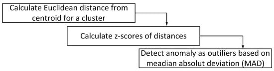
Figure 3.
Procedure to find anomalies within the assigned clusters.
AD consists on finding outliers based on relative ED within each cluster per the following steps: calculate ED of each observation to the centroid; calculate the z-score of such ED values; determine which observation distance represents an outlier by median absolute deviation (MAD). As is known, with the median being a robust estimator of location, MAD is a robust measure of the variability and scale of a data sample [60]. Observations with a distance from the median greater than are considered anomalies, following the criterion set forth in [61], who indicated a factor of 3 as a “very conservative” choice, as also discussed in [62].
Besides already labeled data, new unlabeled data may be screened for anomalies with ED calculation. Based on the same ED, new data may be assigned to an existing cluster, after which the centroid will be updated for the next new observation and its ED value. The process is described in Figure 4.
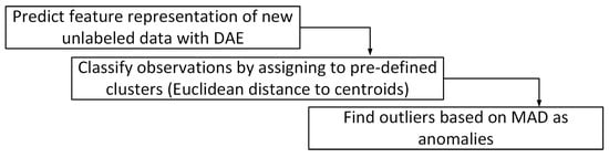
Figure 4.
Classification method based on ED and predefined clusters for unlabeled data.
3.4. 1-D Convolutional Neural Network (CNN)
A more traditional supervised-learning method may be adopted using a 1-D CNN for that portion of data that is labeled (as shown in Figure 5). The dataset is separated for training, validation and testing, allowing assessment of classification performance for the target classes (using confusion matrix and balanced accuracy quantification). Later, the 1-D CNN is also verified on unlabeled data as part of its testing.
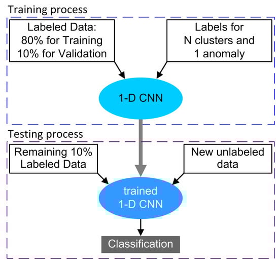
Figure 5.
1-D CNN training and classification process.
DL models based on 1-D CNN are usually composed of the input layer, multiple hidden layers, alternated convolutional and pooling layers, a fully connected layer, and an output layer [63]. In an analog to the popular 2-D CNN, the 1-D CNN allows learning and identification of one-dimensional signals. A comprehensive 1-D CNN description can be found in [12,63], where it was applied to similar tasks of classification of PQ events and fault diagnosis. As inspired by the architecture proposed in [63], the model used in this work is described in Table 2.
Table 2.
CNN Architecture and Training Hyperparameters.
The choice of 1-D CNN is justified not only by its popularity for PQ data classification [36], but also by the following considerations [64].
- Unlike traditional machine learning methods (e.g., support vector machines, k-nearest neighbors, etc.), 1-D CNNs can capture relevant features automatically from raw data during training, which reduces the need for manual work and extensive signal processing for feature extraction.
- Its architecture facilitates learning of local and more abstract features in different steps of the learning process, which helps in identifying complex patterns in the data (human processes or traditional methods are not so effective).
- This leads to the possibility of applying classification to raw data, which is challenging but crucial for identifying waveform distortion patterns directly in the time domain.
4. Results
AC railway data used in this work are taken from a public dataset [65]. They consist of short TD recordings of pantograph current (and voltage) lasting five fundamental cycles (at Hz, this amounts to 300 ms) and selected from much longer recordings. Each of them is tagged with the speed value, the overall absorbed rms current and the specific OCs. The cited source [65] reports information on uncertainty and characteristics and installation of the measuring system.
A set “1” of 5337 waveforms from [65] is used in the following steps: DAE application and clustering for diagnostics and AD, labeling, and training/validation/testing of the CNN. An additional set “2” of 3444 waveforms that neither the DAE model nor the 1-D CNN was trained with is used in the following steps: testing of the classification method based on ED and additional testing for the 1-D CNN. It will be referenced below also as “unlabeled data”, as these waveforms do not belong to the dataset in [65] and are not labeled based on the operating conditions.
At the end, Section 4.6 shows results that validate the methodology for application to other power systems, segmenting unlabeled data related to an EV-charging infrastructure.
4.1. Diagnostic Results from an Unsupervised Learning Method
clusters resulted from set 1 over different OCs and confirm two aspects: WD depends strongly on the OC and NAC is suitable for distortion signature tracking. The results showed five clusters for patterns of non-active current distortion using the five-cycle waveform as input. Those five clusters are distributed across different operating conditions and confirm two aspects: first, the WD dependency on operating conditions, as seen from the non-active current signature of the front-end power converters onboard the rolling stock; second, the feasible usage of non-active current quantities as parameters for load distortion signature identification in AC railways.
Figure 6 shows the patterns for each cluster and their distributions over the input power profile [66]. Cluster 1 (C1) captured patterns of high traction (HT), while Cluster 5 (C5) had medium traction (MT) signatures. There is only one cluster for medium-braking (MB) and high-braking (HB) conditions, i.e., cluster 4 (C4). Cluster 3 (C3) indicates that the patterns for low braking (LB) and low traction (LT) are grouped together, having identified a similar WD behavior (the sign of the power flow is not explicit in ). Cluster 2 (C2) corresponds to the standstill or coasting condition, where auxiliary converters are preponderant and some background distortion is also visible.
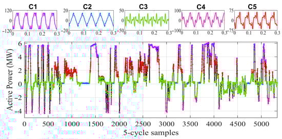
Figure 6.
DAE results showing the NAC 300 ms patterns for the 5 clusters and the cluster distribution over the active power profile.
WD patterns are thus classified with respect to OCs vs. RS active power. However, the diversity and relevance of the clusters, and how the patterns differ from each other, are also crucial aspects that need to be understood. One key method involves evaluating the ED to the cluster centroid.
Figure 7 shows such ED values in matrix form and the ED distribution from the cluster centroid (colored) and from the others (in gray). All clusters have possible outliers that can indicate presence of anomalies within the groups. For C2 (standstill) ED values are all compact and small, showing lack of variability. The physical explanation is that auxiliaries have a steady operating point and that the triangular-like input current (see Figure 6) has a repetitive WD. At the other end, C4 has stronger diversity and is quite dispersed, with large variation in patterns (also visible in the V-I diagrams reported in [14]). One can observe as well that some clusters contain more diversity than others, with this difference reflected in the ED, as for cluster 4. All clusters have possible ED outliers, which can indicate the presence of anomalies.
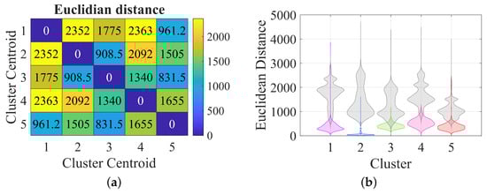
Figure 7.
ED values: (a) between centroids; (b) violin plots of distribution around centroids (Figure 6 colors for the cluster centroids, gray for the others).
Figure 8 shows some examples, where a larger ED value implies more visible deformation. In Figure 8a the ED case is the typical C1 pattern (close to its centroid), whereas the case shows increased high-frequency components. In Figure 8b is caused by evident deformation due to the presence of low-order harmonics. In Figure 8c a substantial variation of the waveform envelope is visible, occurring at both ends of the five-cycle interval (). An evident anomaly with is highlighted in Figure 8d; this is one of the few cases of weird data picked up during the construction of the original dataset [65], and demonstrates the usefulness of the proposed ED screening for large amounts of data.
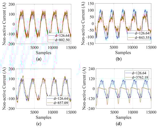
Figure 8.
Waveforms with large ED values for C1: (a) through (d) are different peculiar potential anomaly waveforms with a wide range of ED values.
Figure 9 shows examples for the other clusters, illustrating various changes of shape and underlying causes. In Figure 9a, the traces are similar, but with increasing distortion, as if they describe slightly different behaviors within the same OC merged into the same cluster: as shown in Figure 7b, C4 indeed has intrinsic variability. This is analyzed in more detail in Figure 10, which shows low- and high-order harmonics (up to 2 kHz) and supraharmonics (up to the said kHz):
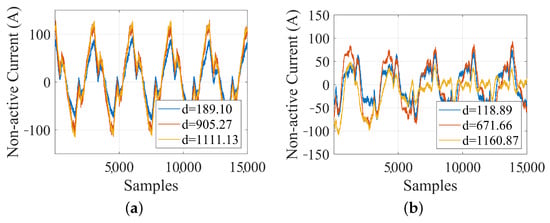
Figure 9.
Waveforms with large ED values for (a) C4 and (b) C5.
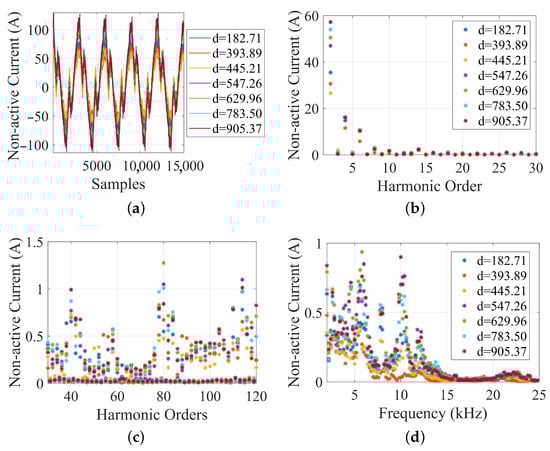
Figure 10.
Waveforms with large ED values for C4 and related harmonic and supraharmonic spectra: (a) waveform examples for different ED, (b) respective harmonic components up to 30th, (c) respective harmonic components between 30th and 120th, and (d) respective supraharmonic spectra.
- all such waveforms show a significant amplitude of fundamental (see Figure 10a), ascribed to the reactive power, so they do not represent low-power transients, e.g., due to uncommon behavior of auxiliaries;
- low-order harmonics are almost absent, as expected for normal operation where the onboard four-quadrant converters (4QCs) follow a policy of cos minimization (see Figure 10b);
- high-order harmonics, instead, are characterized by the switching components of the onboard 4QCs nominally at 800 Hz, so corresponding to the 48th harmonic; their amplitude is in the order of 1 A, , as shown in Figure 10c);
- quite notably the same amplitude can be seen in the lower supraharmonic range, as allowed by the data sampling rate, showing two major peaks at about kHz and 10 kHz, that are only apparently harmonically related, and other minor peaks at kHz and kHz (see Figure 10d); all peaks are confirmed by more than one component coherently indicating amplitudes well above the background level;
- beyond 15 kHz there are no visible spectral signatures, providing an indication of the necessary bandwidth and sample rate.
The natural follow up of the exemplification of large ED values is understanding which ones are really anomalies. This can be achieved without additional post-processing and visual inspection, simply by providing the distribution of the normalized ED values by z-score (see Section 3.3).
Figure 11 illustrates the results for selected clusters indicating which instances are classified as anomalies, found as follows: 14 for C1, 90 for C2, 26 for C3, 12 for C4, and 10 for C5. Those numbers can be related to the previous findings of pertinence and variety within the cluster. C4 (see Figure 11d), for instance, is naturally more dispersed, allowing more variations within the same pattern, which thus has fewer anomalies, while C2 (see Figure 11b) has more anomalies because the pattern is more compact. Another physical explanation associated with anomalies in C2 is the fact that, when there is no significant power absorbed, all usually neglected small emissions from auxiliaries emerge, and the chance of weird oscillations and other uncommon behavior, as well as manoeuvrers (like pantograph down and up, circuit breaker operation, etc.) is more likely.
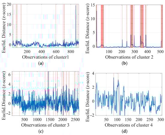
Figure 11.
Anomaly Detection within clusters (time intervals marked in red): (a) C1, (b) C2, (c) C3, (d) C4.
Clustering and AD results proved to segment the input data, which were visualized and validated using OC variations. However, the actual domain of the segmentation happens in the time domain at waveform level, which is challenging due to the nonlinearity and high-dimensionality of such data. This highlights the advantages and potential of the methodology, since single waveform cycles contain the most meaningful, trustworthy and granular representation of electric power systems conditions [67]. Figure 12 illustrates how such segmentation can be visualized, highlighting the distribution of clusters during the NAC variation on a longer time scale, where different OCs follow one to another.
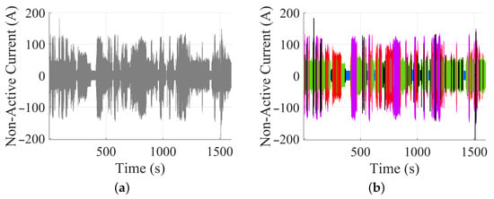
Figure 12.
TD waveform segmentation based on DAE with clusters and AD: (a) raw TD data; (b) segmented data (anomalies coloured as black and cluster separation according to Figure 6).
4.2. Classification Based on ED and Pre-Determined Clusters
The proposed method of Section 3.3 is now evaluated with new unlabeled data (set 2), considering the cluster and anomalies identified as new labels. By applying the workflow of Figure 4, results are obtained as in Figure 13. Since there are predefined cluster labels for the new data, the results are expressed by distributing the classification over the RS power operating points for comparison. At this point, domain knowledge and visualization are essential for interpreting the results.
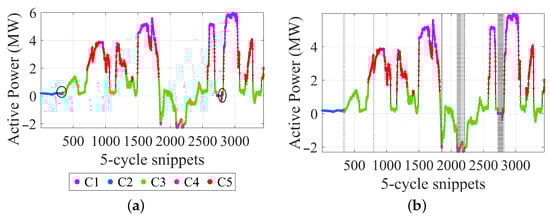
Figure 13.
Classification results based on ED and predetermined clusters: (a) classification based on the predetermined clusters (circles for evident mis-classification); (b) classification with AD (area identified by the dashed horizontal lines).
One can observe from the distribution in Figure 13a that the classification is reasonably coherent with the expected cluster representation according to the OC. Few instances marked with a circle are candidates for mis-classification, where the assigned cluster does not match the associated OC. Additionally, the last step of the ED-based classification, in Figure 4, identifies anomalies, and one can see that those wrong cluster assignments are largely anomalies in the original data. In total, there are 110 anomaly classifications found in the new data, where 4 are for C1, 69 are for C2, 37 for C3, none for C4, and 11 for C5. From a pattern identification viewpoint, those results are interesting since they can be obtained through the well-defined quantity ED, transferring previous knowledge and data classification to new unlabeled data.
4.3. Classification by 1-D CNN with Cluster-Based Labels
The results for set 1, based on clustering and AD, support the creation of labels that impose classes on the data, carrying the association of OCs and WD. The presence of labels opens up the opportunity to train more traditional algorithms like 1-D CNN, as described in Section 3.4. Two points are discussed here: the validation of the labeling process based on DAE feature extraction and clustering, and the performance of the 1-D CNN. After successfully using 80% of the data for training and 10% for validation, the remaining 10% was used for classification and to test the 1-D CNN performance (see the confusion matrix in Figure 14a). The 1-D CNN performs well with the given labels considering the following points: it is an unbalanced set of labels and data with high dimensionality. Considering balanced accuracy (BA), since there is a significant unbalance between classes, the system performed with BA = 89.4% for the test set, in which the anomaly class prevalently pushes down the performance (excluding it, BA = 96.5%).
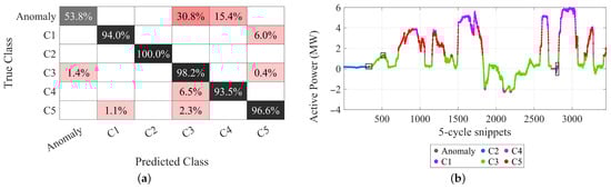
Figure 14.
1-D CNN testing results: (a) test cluster-labelled dataset based on confusion matrix (row-normalized) (b) new unlabelled dataset (squares indicate evident misclassification).
Figure 14b shows the results for the second set 2 of 3444 waveforms of new unlabeled data. Lacking labels to use as reference for verification, comparison with the active power distribution of clusters allows to check that the 1-D CNN classification is reasonable and coherent. A few results deviate from the expected OC associated with that cluster (indicated by squares). Comparing the two methods, as in Figure 15, 84.66% of the 1-D CNN predictions are in agreement with the ED method, without considering anomalies.
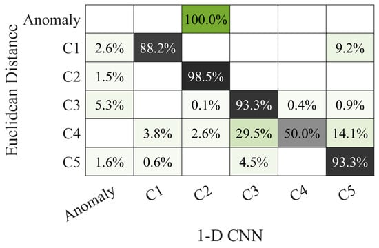
Figure 15.
Confusion matrix (row-normalized) comparing 1-D CNN and ED classification methods.
From a general standpoint nearly 90% of accuracy, 96.5% excluding anomalous cases, using real data in unsupervised learning conditions, is a significant performance, if we compare to other previous works also using TD waveforms, but in supervised learning conditions:
- Ref. [13] reports quite a variable accuracy for the various classes of the PLAID dataset, ending in 81% of balanced accuracy;
- Ref. [37] shows values of average accuracy between 96.6% and 97.2% when working on the LIT-SIM 5 dataset, that may be considered the closest example in that publication to the present case; other past approaches reported in [37] range between 77.2% and 95.4%.
It is noteworthy the absorption of anomalies identified by the unsupervised ED method into the class C2 of the 1-D CNN method. This is at the base of the different scoring of performance with and without the anomaly category.
For more insight in the performance of the 1-D CNN model, the gradient-weighted class activation mapping (Grad-CAM) [68] can be employed for interpretation, by highlighting the data segments that are key to classification [69], measuring their informative content.
Figure 16 shows three examples of correct prediction for C1, C3 and C4.
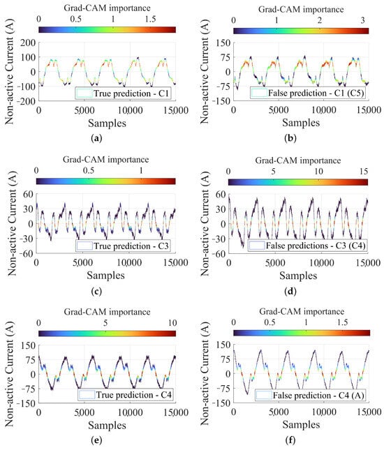
Figure 16.
Explanation of some test prediction of the 1-D CNN using Grad-CAM for correct classifications: (a) true prediction for C1, (b) false prediction for C1, (c) true prediction for C3, (d) false prediction for C3, (e) true prediction for C4, (f) false prediction for C4.
In the case of the C1 prediction (see Figure 16a), the highest importance is highlighted in particular for the top and intermediate parts of the waveform shape, indicating that those segments are more important to determine C1 prediction. The highest value of Grad-CAM importance is 1.84, while the average is 0.68. In that case, 53.4% of the input signal is above the mean value. That signal characteristic can be associated with the high levels of third harmonic in HT conditions, impacting significantly on the TD shape. It is remarkable that the bottom part of each waveform period is not picked up by Grad-CAM: the symmetry of the waveform can be observed, so that probably that part of the waveform is just specular and does not add any innovative information.
Looking at the C4 case (see Figure 16e), the most meaningful waveform segment identified by the Grad-CAM is the zero crossing and an almost 50% of amplitude range around it. That might be associated with the change in the zero crossing direction due to regenerative braking; the prominent distortion around the zero crossing is shared in reality with C3 (see Figure 16c), which has the largest distortion to the point that the waveform shape is quite different almost completely dominated by the 3rd harmonic. For C4, the highest importance value was 10.25, with an average of 1.56. Although the average is significantly lower than the peak, only 26.6% of the waveform exceeds the average, indicating that these segments have a strong influence on the prediction.
All the three insets on the left side of Figure 16 discussed above for C1, C3 and C4 are sided by an example of false prediction (or, misclassification), showing the similarity and closeness of the waveform shape and distortion features. Although the waveforms for C3 in Figure 16c,d may appear visually similar to justify the assignment to the same class (namely C3), Figure 16d actually marks the transition for a new operating state (i.e., C4), as can be evidenced by the increased peak amplitudes and slight change on waveform distortion. This part is particularly challenging due to the similarity of its characteristics to those observed at the limits of normal operating conditions, leading to greater confusion during classification by supervised models as 1-D CNN. It is important to remember that the used labels are not derived from an external or predefined criterion, but are instead the result of clustering based on features extracted by the DAE. This inherently introduces a degree of imprecision into the labeling process, as previously demonstrated with “diagnosis” based on ED. In the case of the C4 class and its corresponding false prediction (Figure 16e and Figure 16f, respectively) it is possible to see that an apparently C4 waveform was classified as “Anomaly”, possibly because of larger high-frequency content, visible in the double “tooth” in the hump above the zero crossing, whereas only one larger tooth is visible in the C4 waveform on the left.
These Grad-CAM examples show that the 1-D CNN model can understand nuances within the input data signals and exploit them to classify, while providing an indication of the relative importance of even small waveform portions. They also demonstrate how the model can shift its attention across the signal, which can be insightful for complex multi-class classification tasks. The attention aspects, associated with WD identification, further enhance the explicability of the analysis (crucial aspect within multi-domain application, as pointed out in [70] for a similar application regarding power system transients).
4.4. Noise and Noise Effect
Some considerations are provided on the noise concept for the method. The experimental data utilized in the work are already characterised by their own intrinsic electric noise that is evaluated in the following to support the statement that the proposed method is robust to data noise. Shifting to a frequency-domain interpretation, the NAC spectrum is evaluated for the characteristic harmonic components compared to the adjacent incoherent spectral frequency bins, assessing what is the amount of noise present in the data as input to the DAE (see Figure 17).
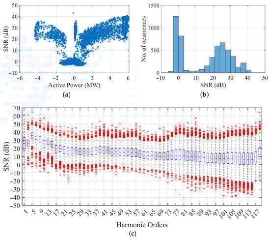
Figure 17.
Signal-to-noise ratio (SNR) distribution in form of box-plots of the input NAC data: (a) SNR vs. input active power; (b) histogram of SNR values; (c) SNR distribution for the odd harmonics of the spectrum up to harmonic order 119 (in the boxplot the blue box extends from the first to the third quartile, the horizontal red dash in the middle is the median, and the remaining red crosses are outliers).
It is possible to see in Figure 17c that the fundamental and low-order harmonics are characterized by a 25–35dB average SNR, whereas beyond the 17th component, included, the SNR settles to about 20 dB going down smoothly to about 10 dB. This is confirmed by the histogram of values in Figure 17b, where altogether they span between 5 and 40 dB, excluding the two tall bins around 0.
These SNR values demonstrate how the proposed unsupervised method can deal with a significant amount of intrinsic noise in the data. The negative values occurring at low power levels are due to the operation of the traction converters in an irrelevant operating region, featuring an overlap of distortion caused by onboard auxiliaries that is not associated with the main characteristic harmonics. The many outliers (shown as red crosses in Figure 17c) demonstrate the highly variable dynamic conditions.
The two classification methods explored in this work were then evaluated by injecting additional artificial incoherent noise (white noise), thereby worsening the SNR values and assessing the consequent performance. The affected components were those with the largest SNR values, thereby reducing the SNR values globally to less than 20 dB (18 dB on average, to be precise), implying a degradation of 12 ± 5 dB.
The aim is to observe any possible shifts in the decision criteria and label assignment during the segmentation of the “unlabeled data” in set 2 (see Figure 18). The results comparing the ED-based classification with and without additional noise are illustrated in Figure 18a. Additionally, the ED classification is compared again to the output of the supervised 1D-CNN model, and the results are presented in Figure 18b.
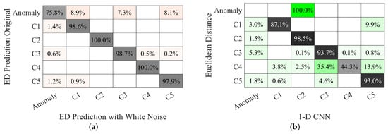
Figure 18.
Confusion matrices for ED unsupervised method operation after injection of additional noise reducing the SNR values below 20 dB: (a) comparison with performance without noise injection (original SNR); (b) comparison with the 1D-CNN classification both with the said additional injected noise. Colours are chosen to visually distinguish the two cases and darker nuances underline higher values.
As shown in Figure 18a there is substantial agreement on the class assignments, with a maximum deviation of 2.1%. Anomalies are instead more dispersed, with some “leakage” (although less than 10%) to the classes C1 through C5 as a result of of noise hitting specific waveform portions, such as the top- and zero-crossings.
4.5. Computational Times
This brief section discusses the computational time needed for the proposed unsupervised DAE method using ED, including a comparison to the computational time needed for the 1D-CNN. Results are shown in Figure 19 and show that the proposed method is much faster and suitable for a real-time implementation, with the most likely value being ms; all values are within ms, with a maximum value of ms at 99% probability. The dispersion of computational times is caused by other concurrent processes on the hosting computer, so the fastest times (which also correspond to the mode of the distributions) provide the best estimate of the computational effort of the algorithm alone.
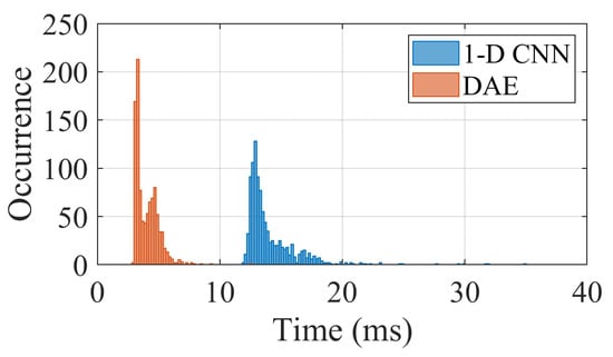
Figure 19.
Distribution of the computational times for 1000 tests of the unsupervised DAE method and 1D-CNN reference method.
4.6. Application with EV Charging Data for Validation
As additional verification, the method has been applied to data measured on the AC side of a 150 kW CCS charging station of a winter car-testing center in the north of Sweden [71]. Several charging sessions lasting several days were recorded by sampling at 40 kHz from the AC feeding lines upstream: the incoming power and associated NAC were then analyzed. Depending on the model of the charging EV, power may vary between 25 kW and 150 kW; the charging times vary from as fast as 6 min to 3 h. Data were recorded as short 500 ms records every minute using Rogowski current sensors. In total, 3338 snippets were captured and used in the proposed methodology. The objective is to validate the method discussed so far by applying it to a completely new scenario, EV charging, which carries significant applicability potential.
Clustering was performed on four classes, which led to the identification of one class involved in the charging at the highest power level (C1), with the two others involved at lower power levels (C3 and C4). The background noise with no EV charging was captured by C2. The in-feed active power is plotted vs. time in Figure 20c, together with the four identified TD patterns. It is possible to see that C2 consistently tags all background noise samples, whereas C1 is reserved for high-power charging, occurring just above 100 kW; the charging session on 10 February, carried out up to 100 kW, in fact, did not yield any C1 pattern.
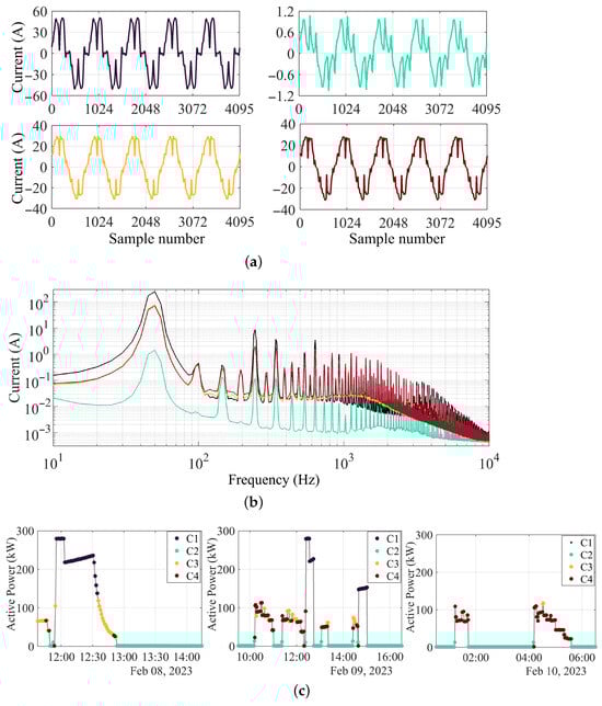
Figure 20.
Verification of EV CCS charging sessions for 3 consecutive days using the proposed method: (a) 100 ms long pattern waveforms of each NAC cluster (sample number on the time axis); (b) corresponding current spectrum up to 10 kHz; (c) distribution of clusters over the active power profile.
The spectra of the total current up to 10 kHz for the respective clusters are also illustrated. It is possible to see that C3 and C4 are very similar, with a slightly larger high-frequency content for C4. C1 is characterized by the largest emissions, these being approximately four times larger than those of C3 and C4 for the first characteristic harmonics (the 5th, 7th and 11th are particularly visible in Figure 20b). The background noise in between the harmonics of the fundamental is almost the same for all modes when charging takes place (C1, C3 and C4), with a slight reduction for C1 between 800 Hz and 2 kHz.
Classification is consistent for the whole 3 days of operation used and reported as an example.
5. Conclusions
The work explored Fryze’s TD NAC to assess the signature of distorting loads (AC railway RS and its onboard converters in the studied case, with the inclusion of an additional case of a CCS EV charging station for confirmation). The challenging aspects arise from the RS’s highly dynamic behavior, as it passes through a wide range of power levels while tractioning and braking. Peculiar WD can be associated with the varying OCs, as confirmed by the analysis of the frequency spectra.
Unsupervised deep learning was used with waveform samples as input. This is a first point of novelty, as it focuses on the informative NAC rather than using the entire V-I trajectory. The exploration of an unsupervised method using unlabeled data is also noteworthy, in particular as it considers the achieved high classification score, providing an interesting solution for the management of new loads, like those seen in electromobility scenarios.
The application of DAE and clustering has identified patterns associated with RS OCs, thereby showing the suitability of for pattern identification and advanced monitoring. ED was explored to evaluate cluster dispersion, and a new method was proposed for identifying anomalies, input WD samples without defined criteria (so, “outliers”), and unusual shapes. New data are then classified based on ED. Results were validated by showing the distribution of classification indexes over the RS OCs; this way, one can confirm the correctness of the data segmentation by its evident coherence with operation and plausibility.
Later, the dataset [65] with cluster-based labels was used for supervised learning with the 1-D CNN to compare results based on ED. BA achieves 96.5% agreement using the testing portion of this dataset. When exposed to new unlabeled data, the 1D-CNN achieves 89.6% agreement with the ED-based method for normal states. Additionally, Grad-CAM was applied to the 1D-CNN model to quantify the importance of waveform segments for prediction and highlight the different attention mechanisms depending on the observed OC.
We here highlight that the work uses clustering and ED to evaluate real-world PQ measurements and that the proposed methodology is capable not only of finding patterns in WD data, but also of addressing uncertainty and inherent variability of the dataset. In other words, it is possible to quantify the quality and consistency of observations, screening to isolate bad, weird or simply unusual data (a feature that is extremely useful with unsupervised measurement and monitoring and big-data analytics). In the studied case, a few records were identified as having anomalous shapes that were not caught earlier by the manual check carried out to build the original dataset in [65], thereby demonstrating the practical validity of the method.
In addition, by classifying new data, this work showed the potential of this approach for transferring knowledge and feature learning to other similar datasets.
Possible applications of this method include NILM aimed at the identification and classification of loads by their distortion signatures, as well as the evaluation of PQ from unsupervised long-term measurements for identification of outliers and weird data. The range of high-power distorting loads and sources encompasses industrial drives, such as those for large fans, pumps, compressors and other motor applications. They are interfaced to the AC grid with converters that are either more traditional diode or thyristor rectifiers or advanced active rectifiers of the same type as the RS 4QC considered here.
For modern renewable sources, such as photovoltaic parks, the AC grid interface is implemented with an inverter with a grid-forming or grid-following operation. The principle of operation is quite similar to that of the 4QC, having similar modulation and switching patterns.
As anticipated, the method has been successfully applied also to a different scenario for further verification: the charging patterns of a CCS charging station were consistently classified over sessions lasting several days. This provides evidence for confidence in applying the method to the forthcoming test campaigns of the Met4EVCS project [72], which focus on conducted emissions and distortion caused by EV charging stations.
Besides the advantages visualized by the results, some considerations related to possible limitations and negative aspects are highlighted below.
- Cluster-based labels are effective in capturing the operational states and load characteristics, enabling other classification algorithms to benefit from the structured data. However, the anomaly category should be used with caution, as it is based on previously known anomalies and may not represent new or previously unseen events. In such cases, the proposed ED-based classification method becomes important again, as it allows the identification of new anomalies that do not conform to existing cluster boundaries.
- Additionally, the success of cluster-based segmentation and labeling remains highly dependent on the clustering algorithm used, which in turn is determined by the data characteristics and the distribution of the data in the feature space.
- Other limitations can be noted regarding the WD signature used. NAC is more suitable for loads with strong non-linear behavior, so its performance may be limited in systems with low non-linearity and distortion. On examination of the results in the literature, it is easy to see that, currently, the category of distorting loads is much broader than that of linear loads, which are mostly limited to heating elements, some home appliances, and a few others.
Author Contributions
Conceptualization, A.M., R.S.S. and S.K.R.; methodology A.M., R.S.S. and S.K.R.; validation, A.M. and R.S.S.; formal analysis, A.M. and R.S.S.; investigation, A.M. and R.S.S.; resources, A.M., R.S.S. and S.K.R.; data curation, A.M. and R.S.S.; writing—original draft, A.M. and R.S.S.; writing—review and editing, A.M., R.S.S. and S.K.R.; visualization, A.M. and R.S.S.; supervision S.K.R.; project administration, A.M. and S.K.R.; funding acquisition, A.M. and S.K.R. All authors have read and agreed to the published version of the manuscript.
Funding
The work here presented has received funding from EPM (European Partnership on Metrology) SRTi03 Met4EVCS. The project SRTi03 Met4EVCS has received funding from the European Partnership on Metrology, co-financed by the European Union’s Horizon Europe Research and Innovation Programme and by the Participating States. This work is also partially funded by the Swedish Transport Administration.
Institutional Review Board Statement
Not applicable.
Informed Consent Statement
Not applicable.
Data Availability Statement
Data are contained within the article.
Conflicts of Interest
The authors declare no conflict of interest.
References
- Shojaie, M.; Mokhtari, H. A method for determination of harmonics responsibilities at the point of common coupling using data correlation analysis. IET Gener. Transm. Distrib. 2014, 8, 142–150. [Google Scholar] [CrossRef]
- Safargholi, F.; Malekian, K.; Schufft, W. On the Dominant Harmonic Source Identification—Part I: Review of Methods. IEEE Trans. Power Deliv. 2018, 33, 1268–1277. [Google Scholar] [CrossRef]
- Bhende, C.; Mishra, S.; Panigrahi, B. Detection and classification of power quality disturbances using S-transform and modular neural network. Electr. Power Syst. Res. 2008, 78, 122–128. [Google Scholar] [CrossRef]
- Panigrahi, B.; Dash, P.; Reddy, J. Hybrid signal processing and machine intelligence techniques for detection, quantification and classification of power quality disturbances. Eng. Appl. Artif. Intell. 2009, 22, 442–454. [Google Scholar] [CrossRef]
- Li, P.; Ma, T.; Shi, J.; Jia, Q. Multi-dimensional feature multi-classifier synergetic classification method for power quality disturbances. Comput. Electr. Eng. 2024, 120, 109720. [Google Scholar] [CrossRef]
- Jain, S.K.; Singh, S.N. Fast Harmonic Estimation of Stationary and Time-Varying Signals Using EA-AWNN. IEEE Trans. Instrum. Meas. 2013, 62, 335–343. [Google Scholar] [CrossRef]
- Moradifar, A.; Akbari Foroud, A.; Fouladi, M. Identification of multiple harmonic sources in power system containing inverter—Based distribution generations using empirical mode decomposition. IET Gener. Transm. Distrib. 2019, 13, 1401–1413. [Google Scholar] [CrossRef]
- Katic, V.A.; Stanisavljevic, A.M. Smart Detection of Voltage Dips Using Voltage Harmonics Footprint. IEEE Trans. Ind. Appl. 2018, 54, 5331–5342. [Google Scholar] [CrossRef]
- de Aguiar, E.; Lazzaretti, A.; Mulinari, B.; Pipa, D. Scattering Transform for Classification in Non-Intrusive Load Monitoring. Energies 2021, 14, 6796. [Google Scholar] [CrossRef]
- Chen, Z.M.; Li, M.S.; Ji, T.Y.; Wu, Q.H. Detection and classification of power quality disturbances in time domain using probabilistic neural network. In Proceedings of the International Joint Conference on Neural Networks (IJCNN), Vancouver, BC, Canada, 24–29 July 2016; pp. 1277–1282. [Google Scholar] [CrossRef]
- Wang, S.; Chen, H. A novel deep learning method for the classification of power quality disturbances using deep convolutional neural network. Appl. Energy 2019, 235, 1126–1140. [Google Scholar] [CrossRef]
- Liu, F.; Zhou, F.; Ma, L. An Automatic Detection Framework for Electrical Anomalies in Electrified Rail Transit System. IEEE Trans. Instrum. Meas. 2023, 72, 3510313. [Google Scholar] [CrossRef]
- Zhou, Z.; Xiang, Y.; Xu, H.; Wang, Y.; Shi, D. Unsupervised Learning for Non-intrusive Load Monitoring in Smart Grid Based on Spiking Deep Neural Network. J. Mod. Power Syst. Clean Energy 2022, 10, 606–616. [Google Scholar] [CrossRef]
- Salles, R.S.; De Oliveira, R.A.; Rönnberg, S.K.; Mariscotti, A. Data-driven assessment of VI diagrams for inference on pantograph quantities waveform distortion in AC railways. Comput. Electr. Eng. 2024, 120, 109730. [Google Scholar] [CrossRef]
- Ur Rehman, A.; Tjing Lie, T.; Valles, B.; Rahman Tito, S. Comparative Evaluation of Machine Learning Models and Input Feature Space for Non-intrusive Load Monitoring. J. Mod. Power Syst. Clean Energy 2021, 9, 1161–1171. [Google Scholar] [CrossRef]
- Angelis, G.F.; Timplalexis, C.; Krinidis, S.; Ioannidis, D.; Tzovaras, D. NILM applications: Literature review of learning approaches, recent developments and challenges. Energy Build. 2022, 261, 111951. [Google Scholar] [CrossRef]
- Liu, Y.; Wang, Y.; Ma, J. Non-Intrusive Load Monitoring in Smart Grids: A Comprehensive Review. Available online: https://arxiv.org/abs/2403.06474 (accessed on 20 June 2025).
- Kerk, S.G.; Hassan, N.U.; Yuen, C. Smart Distribution Boards (Smart DB), Non-Intrusive Load Monitoring (NILM) for Load Device Appliance Signature Identification and Smart Sockets for Grid Demand Management. Sensors 2020, 20, 2900. [Google Scholar] [CrossRef]
- Stanescu, D.; Enache, F.; Popescu, F. Smart Non-Intrusive Appliance Load-Monitoring System Based on Phase Diagram Analysis. Smart Cities 2024, 7, 1936–1949. [Google Scholar] [CrossRef]
- Shen, Y.; Abubakar, M.; Liu, H.; Hussain, F. Power Quality Disturbance Monitoring and Classification Based on Improved PCA and Convolution Neural Network for Wind-Grid Distribution Systems. Energies 2019, 12, 1280. [Google Scholar] [CrossRef]
- Shklyarskiy, Y.; Hanzelka, Z.; Skamyin, A. Experimental Study of Harmonic Influence on Electrical Energy Metering. Energies 2020, 13, 5536. [Google Scholar] [CrossRef]
- Have, B.t.; Azpurua, M.A.; Hartman, T.; Pous, M.; Moonen, N.; Silva, F.; Leferink, F. Waveform Model to Characterize Time-Domain Pulses Resulting in EMI on Static Energy Meters. IEEE Trans. Electromagn. Compat. 2021, 63, 1542–1549. [Google Scholar] [CrossRef]
- Loschi, H.; Nascimento, D.; Smolenski, R.; Sayed, W.E.; Lezynski, P. Shaping of converter interference for error rate reduction in PLC based smart metering systems. Measurement 2022, 203, 111946. [Google Scholar] [CrossRef]
- Mariscotti, A.; Mingotti, A. The Effects of Supraharmonic Distortion in MV and LV AC Grids. Sensors 2024, 24, 2465. [Google Scholar] [CrossRef] [PubMed]
- Kommey, B.; Tamakloe, E.; Kponyo, J.J.; Tchao, E.T.; Agbemenu, A.S.; Nunoo-Mensah, H. An artificial intelligence-based non-intrusive load monitoring of energy consumption in an electrical energy system using a modified K-Nearest Neighbour algorithm. IET Smart Cities 2024, 6, 132–155. [Google Scholar] [CrossRef]
- Mariscotti, A. Impact of Harmonic Power Terms on the Energy Measurement in AC Railways. IEEE Trans. Instrum. Meas. 2020, 69, 6731–6738. [Google Scholar] [CrossRef]
- Mishra, M.; Nayak, J.; Naik, B.; Abraham, A. Deep learning in electrical utility industry: A comprehensive review of a decade of research. Eng. Appl. Artif. Intell. 2020, 96, 104000. [Google Scholar] [CrossRef]
- Sima, W.; Zhang, H.; Yang, M.; Yuan, T.; Sun, P.; Chen, Q.; Zhao, H. A framework for automatically cleansing overvoltage data measured from transmission and distribution systems. Int. J. Electr. Power Energy Syst. 2018, 102, 381–392. [Google Scholar] [CrossRef]
- Oliver, A.; Odena, A.; Raffel, C.A.; Cubuk, E.D.; Goodfellow, I. Realistic evaluation of deep semi-supervised learning algorithms. Adv. Neural Inf. Process. Syst. 2018, 31, 3239–3325. [Google Scholar]
- Zhang, C.; Bengio, S.; Hardt, M.; Recht, B.; Vinyals, O. Understanding deep learning (still) requires rethinking generalization. Commun. ACM 2021, 64, 107–115. [Google Scholar] [CrossRef]
- Raygani, S.; Tahavorgar, A.; Fazel, S.; Moaveni, B. Load flow analysis and future development study for an AC electric railway. IET Electr. Syst. Transp. 2012, 2, 139. [Google Scholar] [CrossRef]
- Salles, R.S.; de Oliveira, R.A.; Ronnberg, S.K.; Mariscotti, A. Analytics of Waveform Distortion Variations in Railway Pantograph Measurements by Deep Learning. IEEE Trans. Instrum. Meas. 2022, 71, 2516211. [Google Scholar] [CrossRef]
- Hu, Z.; Han, Y.; Zalhaf, A.S.; Zhou, S.; Zhao, E.; Yang, P. Harmonic Sources Modeling and Characterization in Modern Power Systems: A Comprehensive Overview. Electr. Power Syst. Res. 2023, 218, 109234. [Google Scholar] [CrossRef]
- Mariscotti, A. Non-Intrusive Load Monitoring Applied to AC Railways. Energies 2022, 15, 4141. [Google Scholar] [CrossRef]
- Hassan, T.; Javed, F.; Arshad, N. An Empirical Investigation of V-I Trajectory Based Load Signatures for Non-Intrusive Load Monitoring. IEEE Trans. Smart Grid 2014, 5, 870–878. [Google Scholar] [CrossRef]
- de Oliveira, R.A.; Bollen, M.H. Deep learning for power quality. Electr. Power Syst. Res. 2023, 214, 108887. [Google Scholar] [CrossRef]
- Mulinari, B.M.; da Silva Nolasco, L.; Oroski, E.; Lazzaretti, A.E.; Linhares, R.R.; Renaux, D.P.B. Feature Extraction of V–I Trajectory Using 2-D Fourier Series for Electrical Load Classification. IEEE Sens. J. 2022, 22, 17988–17996. [Google Scholar] [CrossRef]
- Han, Y.; Li, K.; Feng, H.; Zhao, Q. Non-intrusive load monitoring based on semi-supervised smooth teacher graph learning with voltage–current trajectory. Neural Comput. Appl. 2022, 34, 19147–19160. [Google Scholar] [CrossRef]
- Salles, R.S.; Rönnberg, S.K. Review of Waveform Distortion Interactions Assessment in Railway Power Systems. Energies 2023, 16, 5411. [Google Scholar] [CrossRef]
- Fryze, S. Wirk, Blind, un Scheinleitung in elektrischen Stromkreisen mitnichtsinusoidalem Verlauf von Strom und Spanung. Elektrotechnischen Zeitschrift 1932, 25, 26, 29, 1–8. [Google Scholar]
- Späth, H. A general purpose definition of active current and non-active power based on German standard DIN 40110. Electr. Eng. 2005, 89, 167–175. [Google Scholar] [CrossRef]
- EN 50163; Railway Applications—Supply Voltages of Traction Systems. CENELEC: Brussels, Belgium, 2020.
- Mousavi Gazafrudi, S.M.; Tabakhpour Langerudy, A.; Fuchs, E.F.; Al-Haddad, K. Power Quality Issues in Railway Electrification: A Comprehensive Perspective. IEEE Trans. Ind. Electron. 2015, 62, 3081–3090. [Google Scholar] [CrossRef]
- EN 50388-1; Railway Applications—Fixed Installationsand Rolling Stock—Technical Criteria for the Coordination Between Electric Traction Power Supply Systems and Rolling Stock to Achieve Interoperability. CENELEC: Brussels, Belgium, 2022.
- Bongiorno, J.; Bhagat, S. Accuracy and Repeatability of Rolling Stock Current Distortion Tests for Interference to Signalling. Metrology 2025, 5, 17. [Google Scholar] [CrossRef]
- Liu, Q.; Zhang, W.; Cao, G.; Liu, J.; Ye, J.; Wu, M.; Yang, S. Influence of the Catenary Distributed Parameters on the Resonance Frequencies of Electric Railways Based on Quantitative Calculation and Field Tests. Energies 2022, 15, 3752. [Google Scholar] [CrossRef]
- He, F.; Li, Z.; Zhang, H.; Ai, L.; Hu, H. Parallel Harmonic Resonance Probability Identification of Traction Power Supply System Based on Measured Data. Dianwang Jishu/Power Syst. Technol. 2024, 48, 2084–2094. [Google Scholar] [CrossRef]
- Hinton, G.E.; Salakhutdinov, R.R. Reducing the Dimensionality of Data with Neural Networks. Science 2006, 313, 504–507. [Google Scholar] [CrossRef]
- Dong, G.; Liao, G.; Liu, H.; Kuang, G. A Review of the Autoencoder and Its Variants: A Comparative Perspective from Target Recognition in Synthetic-Aperture Radar Images. IEEE Geosci. Remote Sens. Mag. 2018, 6, 44–68. [Google Scholar] [CrossRef]
- Singhal, A. Modern information retrieval: A brief overview. IEEE Data Eng. Bull. 2001, 24, 35–43. [Google Scholar]
- Sugato, B.; Mikhail, B.; Arindam, B.; Raymond, M. Probabilistic Semi-Supervised Clustering with Constraints. In Semi-Supervised Learning; The MIT Press: Cambridge, MA, USA, 2006; pp. 73–102. [Google Scholar] [CrossRef]
- Yao, G.; Wu, Y.; Huang, X.; Ma, Q.; Du, J. Clustering of Typical Wind Power Scenarios Based on K-Means Clustering Algorithm and Improved Artificial Bee Colony Algorithm. IEEE Access 2022, 10, 98752–98760. [Google Scholar] [CrossRef]
- Sinaga, K.P.; Yang, M.S. Unsupervised K-Means Clustering Algorithm. IEEE Access 2020, 8, 80716–80727. [Google Scholar] [CrossRef]
- Islam, M.M.; Faruque, M.O.; Butterfield, J.; Singh, G.; Cooke, T.A. Unsupervised clustering of disturbances in power systems via deep convolutional autoencoders. In Proceedings of the IEEE Power & Energy Society General Meeting (PESGM), Orlando, FL, USA, 16–20 July 2023; pp. 1–5. [Google Scholar] [CrossRef]
- Calinski, T.; Harabasz, J. A dendrite method for cluster analysis. Commun. Stat. Theory Methods 1974, 3, 1–27. [Google Scholar] [CrossRef]
- Mariscotti, A. Behavior of single-point harmonic producer indicators in electrified AC railways. Metrol. Meas. Syst. 2020, 27, 641–657. [Google Scholar] [CrossRef]
- Ciancetta, F.; Bucci, G.; Fiorucci, E.; Mari, S.; Fioravanti, A. A New Convolutional Neural Network-Based System for NILM Applications. IEEE Trans. Instrum. Meas. 2021, 70, 1501112. [Google Scholar] [CrossRef]
- Teshome, D.; Huang, T.D.; Lian, K.L. A Distinctive Load Feature Extraction Based on Fryze’s Time-domain Power Theory. IEEE Power Energy Technol. Syst. J. 2016, 3, 60–70. [Google Scholar] [CrossRef]
- Mylona, D.N.; Bouhouras, A.S. A digital twin-based framework for load identification using odd harmonic current plots. Appl. Intell. 2025, 55, 635. [Google Scholar] [CrossRef]
- Pham-Gia, T.; Hung, T. The mean and median absolute deviations. Math. Comput. Model. 2001, 34, 921–936. [Google Scholar] [CrossRef]
- Miller, J. Short Report: Reaction Time Analysis with Outlier Exclusion: Bias Varies with Sample Size. Q. J. Exp. Psychol. Sect. A 1991, 43, 907–912. [Google Scholar] [CrossRef]
- Leys, C.; Ley, C.; Klein, O.; Bernard, P.; Licata, L. Detecting outliers: Do not use standard deviation around the mean, use absolute deviation around the median. J. Exp. Soc. Psychol. 2013, 49, 764–766. [Google Scholar] [CrossRef]
- Huang, D.; Li, S.; Qin, N.; Zhang, Y. Fault Diagnosis of High-Speed Train Bogie Based on the Improved-CEEMDAN and 1-D CNN Algorithms. IEEE Trans. Instrum. Meas. 2021, 70, 3508811. [Google Scholar] [CrossRef]
- Kiranyaz, S.; Avci, O.; Abdeljaber, O.; Ince, T.; Gabbouj, M.; Inman, D.J. 1D convolutional neural networks and applications: A survey. Mech. Syst. Signal Process. 2021, 151, 107398. [Google Scholar] [CrossRef]
- Mariscotti, A. Data sets of measured pantograph voltage and current of European AC railways. Data Brief 2020, 30, 105477. [Google Scholar] [CrossRef]
- Mariscotti, A.; Salles, R.S.; Rönnberg, S.K. Time-Domain Power Theory Applied to Waveform Distortion Assessment of AC Railways. In Proceedings of the IEEE 14th International Workshop on Applied Measurements for Power Systems (AMPS), Caserta, Italy, 18–20 September 2024; Volume 7, pp. 1–6. [Google Scholar] [CrossRef]
- Xu, W.; Huang, Z.; Xie, X.; Li, C. Synchronized Waveforms—A Frontier of Data-Based Power System and Apparatus Monitoring, Protection, and Control. IEEE Trans. Power Deliv. 2022, 37, 3–17. [Google Scholar] [CrossRef]
- Selvaraju, R.R.; Cogswell, M.; Das, A.; Vedantam, R.; Parikh, D.; Batra, D. Grad-CAM: Visual Explanations from Deep Networks via Gradient-Based Localization. In Proceedings of the IEEE International Conference on Computer Vision (ICCV), Venice, Italy, 22–29 October 2017; pp. 618–626. [Google Scholar] [CrossRef]
- Sharan, R.V.; Takeuchi, H.; Kishi, A.; Yamamoto, Y. Macro-Sleep Staging with ECG-Derived Instantaneous Heart Rate and Respiration Signals and Multi-Input 1D CNN-BiGRU. IEEE Trans. Instrum. Meas. 2024, 73, 2535212. [Google Scholar] [CrossRef]
- Chen, Q.; Lin, N.; Bu, S.; Wang, H.; Zhang, B. Interpretable Time-Adaptive Transient Stability Assessment Based on Dual-Stage Attention Mechanism. IEEE Trans. Power Syst. 2023, 38, 2776–2790. [Google Scholar] [CrossRef]
- Nakhodchi, N.; Bollen, M.H. Impact of modelling of MV network and remote loads on estimated harmonic hosting capacity for an EV fast charging station. Int. J. Electr. Power Energy Syst. 2023, 147, 108847. [Google Scholar] [CrossRef]
- 23IND06 Met4EVCS Project. Metrology for Electric Vehicle Charging Systems. 2024. Available online: https://www.vsl.nl/en/met4evcs/ (accessed on 15 May 2025).
Disclaimer/Publisher’s Note: The statements, opinions and data contained in all publications are solely those of the individual author(s) and contributor(s) and not of MDPI and/or the editor(s). MDPI and/or the editor(s) disclaim responsibility for any injury to people or property resulting from any ideas, methods, instructions or products referred to in the content. |
© 2025 by the authors. Licensee MDPI, Basel, Switzerland. This article is an open access article distributed under the terms and conditions of the Creative Commons Attribution (CC BY) license (https://creativecommons.org/licenses/by/4.0/).