Flat vs. Curved: Machine Learning Classification of Flexible PV Panel Geometries

Abstract

As the global demand for clean and sustainable energy grows, photovoltaics (PVs) have become an important technology in this industry. Thin-film and flexible PV modules offer noticeable advantages for irregular surface mounts and mobile applications. This study investigates the use of four machine learning models to detect different flexible PV module geometries based on power output data. Three identical flexible PV modules were mounted in flat, concave, and convex configurations and connected to batteries via solar chargers. The experimental results showed that all geometries fully charged their batteries within 6–7 h on a sunny day with the flat, concave-, and convex-shaped modules achieving a peak power of 95 W. On a cloudy day, the concave and convex modules recorded peak outputs of 72 W and 65 W, respectively. Simulation results showed that the XGBoost model delivered the best classification performance, showing 93% precision with the flat-mounted module and 98% recall across all geometries. In comparison, the KAN model recorded the lowest precision (78%) with the curved geometries. A calibration analysis on the ML models showed that Random Forest and XGBoost were well calibrated for the flat-mounted module. However, they also showed overconfidence and underconfidence issues with the curved module geometries.

1. Introduction

The ever-increasing demand for electrical energy in the industrial, commercial, residential, and even agricultural sectors has pushed clean energy investments to increase, with around 34% of global electricity generation coming from renewable energy sources [1]. In fact, it is projected that almost 90% of global energy generation will come from renewable sources by 2050 [2]. However, the International Energy Agency (IEA) estimates that investments of USD 4 trillion are needed every year in clean energy to reach net zero emissions by 2050 [2]. This has led many industries and researchers to investigate and experiment with several technologies in renewable energy systems.

Photovoltaic (PV) technology is considered one of the most commonly utilized systems in sustainable energy solutions due to its advancements in efficiency and cost reduction which have enabled widespread adoption. For instance, the efficiency of conventional silicon-based solar panels has increased to more than 25% [3], while new technologies, including perovskite and tandem solar cells, offer the potential for even better performance outcomes [4]. However, the efficiency of photovoltaics can be affected by many factors like temperature [5], dust [6], and anomalies like partial and full shade [7].

Furthermore, the rigid nature of conventional PV panels can create difficulties for installation on non-flat surfaces like curved building rooftops, irregular structural elements, and vehicles while also limiting their use in spatially constrained environments. Flexible thin-film photovoltaic panels represent a viable solution to overcome this limitation [8,9,10]. However, installing these flexible PV panels on curved surfaces may present more challenges: a flexible PV panel can be curved such that not all of its surface is exposed to sunlight, hence, reducing its efficiency at particular times of day depending on how it is curved. In some situations, a part of the flexible PV may also cast temporary shade on itself or other adjacent panels [11]. The non-uniform exposure to sunlight could create fluctuations in the performance of flexible PV panels.

Artificial Intelligence (AI) offers a viable solution to this problem by predicting the performance of flexible thin-film PV panels under a variety of curvature circumstances. Machine learning algorithms can assess solar exposure patterns, shading effects, and surface orientations to determine the best and worst installation surfaces.

2. Background

It is well known that solar PV panels are affected by different environmental factors like temperature [12,13], solar radiation, dust [14], and shading [15]. Normally, the effects of these factors may be determined by relying on fixed equations, assumptions, and the expertise of humans [16]. However, with the utilization of large amounts of PV performance data, machine learning (ML) models are considered a more robust approach for the prediction and optimization of solar photovoltaic (PV) panel performance [17]. ML models are able to analyze large and complex datasets, discover trends and anomalies, and predict the solar PV systems’ performances throughout various environmental conditions.

Many ML methods are commonly applied to predict and optimize solar PV panels’ performance [18], the most common of which is Artificial Neural Networks (ANNs) [19,20], which is considered effective for modeling nonlinear relationships between input variables and predicting power output based on environmental factors. However, their effectiveness typically depends on the availability of sufficiently large datasets to avoid overfitting, and they may be less suitable in scenarios where high model interpretability is required, such as in diagnostic or operational decision making contexts. Other ML methods include Support Vector Machines (SVMs) [21], Random Forest (RF) [22], Recurrent Neural Networks (RNNs), and Long Short-Term Memory (LSTM) [23] which are ideal for time series forecasting of solar energy output based on harvested weather and performance data, as well as Gradient Boosting methods (like XGBoost, LightGBM) [24], and many others, depending on the type and complexity of the harvested data.

However, with the continuous advancements of solar PV technologies, ML models become increasingly pivotal in predicting the performance and behavior of newer generations of solar PV panels. For instance, several ML models have been utilized to predict bifacial PV panels’ performances [25]. A previous study developed a bidirectional recurrent neural network to predict the power production of bifacial PV modules [26]. The simulation analyzed their performance under different weather conditions. Another study investigated the performance of bifacials that were installed on flat rooftop buildings using an ANN [27]. The results showed that the ANN model accurately predicted the power output of bifacials when the roof surface albedo increased. A more recent study implemented several ML methods to predict the output power of a 3 kW bifacial system [28]. The results showed the linear regression method delivered the best predictive performance.

The power performance and predictive maintenance of flexible thin-film solar PV panels have also been investigated using ML methods. Mubarak et al. tested multiple ML techniques to predict the power output of a thin-film PV system [29]. Among all tested models, the Extra Tree regression proved to be the most accurate with a mean absolute error of 39%. Similarly, a hybrid ANN model was used to estimate the energy yield of thin-film photovoltaic plants [30]. Furthermore, comparisons between conventional ML techniques and deep learning models in predicting the energy outputs of flexible PV panels have been made [31,32]. The results showed that deep learning outperformed conventional ML methods in terms of accuracy.

Thin-film and flexible solar PV modules are considered advantageous when installations are required on curved and irregular surfaces. However, changing the inclination angle of the module or bending it at extreme angles may affect its power output [33]. The literature shows that many tests have been conducted on the mechanical integrity of flexible thin-film PV modules [9,34]. Though, most of the recent studies have focused on newer module generations like perovskite solar cells [35,36]. Despite the growing interest in machine learning (ML) in solar photovoltaic applications, there is a research gap in its application to flexible thin-film PVs. Specifically, the studies that deploy ML techniques to predict the performance of such modules based on surface shape and curvature are very few, even though predicting the shape and curvature of a PV module can be advantageous to expose the weaknesses and limitations of such systems. This research addresses that gap by deploying ML techniques to predict the geometry and performance of flexible thin-film PV modules. The novelty of this work is showcased in utilizing the curvature of the PV module as one of the parameters that can be integrated into ML models that predict the PV’s electrical behavior. This study not only introduces a new parameter to ML models specialized in flexible thin-film PV modules but also improves the application and use of flexible solar panels in real-world situations.

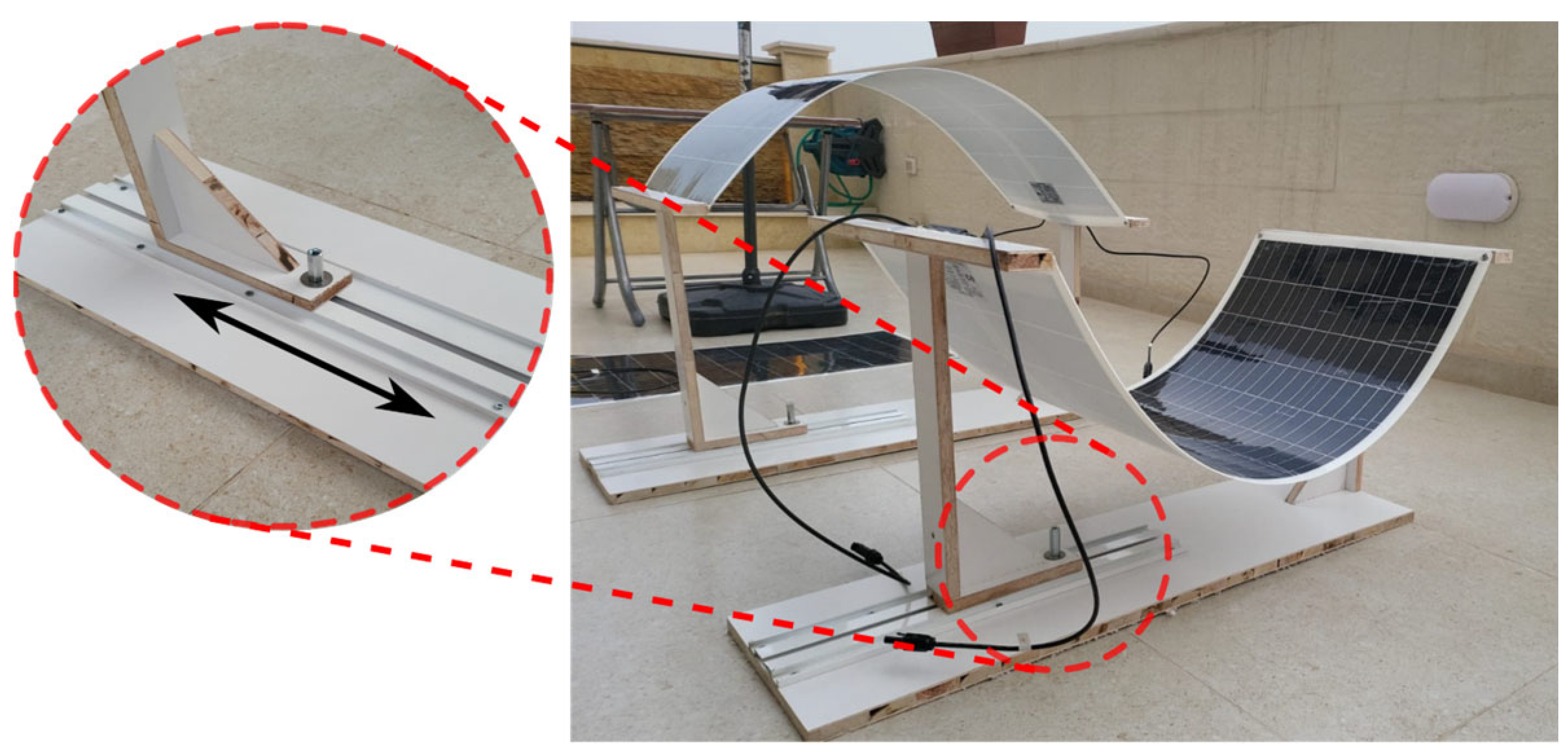
3. Experimental Setup

In this work, an experiment was carried out to evaluate the effects of flexible photovoltaics curvature on battery charging performance in real conditions. Three identical 100 W flexible photovoltaic panels were tested to charge 12 V, 30 A batteries via separate PWM solar chargers (Tarom 4545).

Table 1. Characteristics of the flexible PV module used in this study.

Power	100 [W]
Rated Voltage	18 [V]
Rated Current	5.5 [Amp]
Voc	21.6 [V]
Isc	6.5 [Amp]
Dimensions	1030 × 520 × 2 mm

shows the characteristics of the utilized panels. Two of the panels were configured in the shape of a concave and a convex curve with a 50 cm radius. The third panel was left flat as a control for the experiment.

All three PV panels were mounted facing south for maximum efficiency. Figure 1 shows a schematic drawing of the setup. The apparatus on which the concavely and convexly curved PV panels were mounted was made of wood and could be altered to change the curvatures of the panels via a sliding mechanism as shown in Figure 2.

The setup was exposed to sunlight throughout two inconsecutive days. Day 1 had clear and sunny conditions while day 2 was partly cloudy. Figure 3 shows the recorded sunlight radiation during the two days using a silicon pyranometer (±10 W/m² accuracy). The sunny day data shows a normal distribution of solar intensity where it peaks around solar noon just above 1000 W/m². In contrast, the cloudy day data shows random fluctuations in solar irradiance throughout the day depending on cloud formation on that day. These fluctuations significantly influence the electrical performance of the flexible PV panels, hence, affecting the batteries’ state of charge, SOC.

For each day, the experiment started at 8:00AM using batteries with a state of charge (SOC) of 50%. During the experiment, the panels’ current, voltage, and the batteries’ SOC were recorded in 5 min intervals until 6:00PM to give a total of 120 data entry points. Static electronic loads were connected to the batteries through the chargers, which were activated once the batteries reached a 100% state of charge (SOC). This would eliminate possible current interference with the chargers and reset the batteries’ SOC to 50% for the next experiment. Additionally, the wattage and efficiency (illustrated in Equation (1) [37]) of the panels were calculated throughout the experiment.

$${\eta }_{el}={\displaystyle \frac{P_{mp}}{A_{PV}\times G}}\times 100$$

(1)

Equation (1) represents the electrical efficiency of a solar photovoltaic panel where

• $P_{mp}$ is the maximum power point in [W];
• $A_{PV}$ is the surface area of the photovoltaic panel in [m²];
• $G$ is the solar irradiance in [W/m²].

The purpose of the experiment was to evaluate the effect of a flexible photovoltaic panel’s curvature on its efficiency in a practical situation where a flat-mounted PV panel may not be ideal.

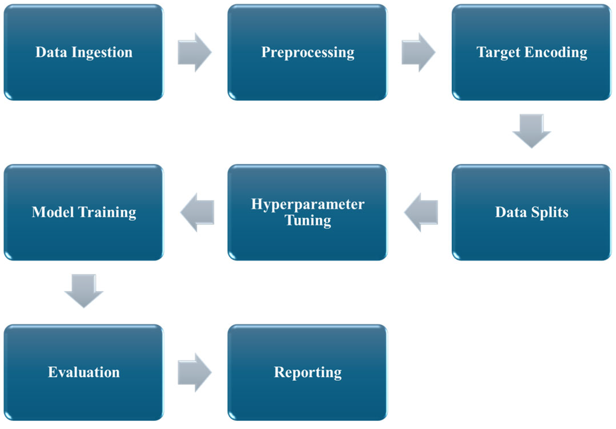
4. Deployed Machine Learning Methods

This section describes the harvested dataset in this study and the machine learning (ML) techniques that were deployed for flexible photovoltaic (PV) performance prediction.

4.1. Data Description

The dataset comprises 726 timestamped measurements of a flexible photovoltaic panel under two weather conditions (“sunny” and “cloudy”). Each record includes eight continuous features—radiation (W/m²), voltage (V), current (A), power (W), state of charge (SOC, %), efficiency (unitless), hour, and minute—plus a one-hot indicator for weather. The target is a three-way classification of the panel’s geometric configuration: flat, concave, or convex. The classes are perfectly balanced (242 samples each with an even 50/50 split between sunny and cloudy conditions), eliminating class-imbalance bias. The time features capture diurnal effects, while the one-hot weather flags allow the models to learn condition-specific performance. The combination of electrical, environmental, and temporal features provides a rich multimodal input for classification.

4.2. Machine Learning Models

In this subsection, we employed four machine learning models: Random Forest (RF), XGBoost, Multi-Layer Perceptron (MLP), and Kolmogorov–Arnold Network (KAN). These models were selected to represent a range of methodologies in terms of complexity and interpretability. Random Forest and XGBoost are well-established methods for structured tabular data, while MLP serves as a deep learning benchmark. KAN, a more recent model, incorporates a non-Euclidean chaotic embedding architecture. The inclusion of these models allowed for a comparison of classical, ensemble, and deep learning approaches. Although other models, such as SVM or MobileNet, are useful—particularly for embedded applications—this study prioritized algorithmic generality and performance clarity on a moderately sized dataset (726 entries).

4.2.1. Random Forest

RF is an ensemble of decision trees trained on bootstrap samples with random feature subsets at each split. By averaging over dozens or hundreds of trees, it reduces variance and avoids overfitting on noisy measurements of power and radiation. It naturally handles nonlinear interactions—e.g., between voltage and efficiency—and gives an intrinsic measure of feature importance. Training and inference are fast, making it a robust baseline. We configured 200 trees with a maximum depth of 8 and sqrt-feature subsampling, which yielded a stable performance across cross-validation folds. Its simplicity and interpretability make it a crucial comparator for more complex methods.

4.2.2. Extreme Gradient Boosting

XGBoost builds trees sequentially, with each one correcting the errors of its predecessors via gradient descent on the multi-class log loss. With built-in regularization (L1/L2), column subsampling, and shrinkage (learning rate), it often outperforms plain Random Forests on structured data. The hyperparameters—tree depth, learning rate, subsample ratios—used are optimized to maximize macro ROC–AUC (receiver operating characteristics–area under the curve). The resulting model achieved the highest accuracy and AUC in our experiments, benefiting from its ability to model subtle feature interactions (e.g., Radiation X Efficiency) and handle outliers gracefully. Its prediction probabilities are well calibrated after tuning, which is critical for downstream decision making.

4.2.3. Kolmogorov–Arnold Network

KAN draws inspiration from dynamical systems theory, notably the Arnold cat map and Kolmogorov flow. It applies learned chaotic embedding to input features, scrambling and reassembling them in a higher-dimensional manifold before classification. This “chaos embedding” can disentangle class clusters that are not linearly separable. Our implementation uses a parameterized Arnold map followed by a linear output layer, trained end-to-end with cross-entropy loss. We employ AdamW optimization, ReduceLROnPlateau scheduling, and early stopping to prevent overfitting. While KAN achieved a respectable macro AUC, it slightly underperformed relative to XGBoost and MLP, indicating the potential for further tuning of its dynamical parameters.

4.2.4. Multi-Layer Perceptron

Our MLP is a three-layer fully connected network (sizes 64→32→3) with batch normalization, ReLU activations, and dropout. It is optimized using AdamW with weight decay and ReduceLROnPlateau scheduling to adapt the step size. The MLP can approximate arbitrary decision boundaries when given enough capacity but requires careful regularization to avoid overfitting on the 726 samples. In practice, it learned meaningful combinations of time, weather, and electrical features, achieving a performance close to KAN. Its end-to-end differentiability and simplicity make it a useful deep learning baseline.

4.2.5. Cross-Validation and Hyperparameter Tuning Strategies

We conducted cross-validation and hyperparameter optimization techniques for assessing the robustness and reproducibility of our results. To this end, we employed a repeated stratified k-fold cross-validation strategy across all models—RF, XGBoost, MLP, and KAN. Specifically, a 5-fold stratified split was repeated twice, ensuring both class balance in each fold and a broader sampling of data partitions. All reported performance metrics, including accuracy, precision, recall, F1 score, and ROC–AUC, were averaged across these 10 runs (5 folds × 2 repeats), offering a reliable estimate of each model’s generalization performance. This stratified and repeated evaluation scheme mitigates the impact of random fluctuations and enhances result stability.

For hyperparameter optimization, XGBoost was tuned using the Optuna framework [38] over 25 trials, with each trial internally validated using 3-fold repeated cross-validation. This allowed us to effectively explore the parameter space and maximize the macro-average ROC–AUC, our optimization target. For KAN and MLP, instead of exhaustive parameter searches, we adopted a robust training based on early stopping—halting training when validation performance settled down—to avoid overfitting. Patience was set to 20 epochs for KAN and 15 for MLP, with dynamic learning rate adjustments guided by validation loss. This strategy, combined with a well-established baseline architecture, offered a practical yet effective balance between training efficiency and performance reliability.

In all four methods, the data was processed according to the simulation pipeline shown in Figure 4.

5. Results

This section presents the results of this study. First, the experimental measurements of the flexible modules’ power output and battery state of charge (SOC) are presented. The second subsection discusses the performance of the presented ML models (i.e., Random Forest, XGBoost, Kernel Adaptive Network, KAN, and Multi-Layer Perceptron, MLP) in predicting the modules’ behavior.

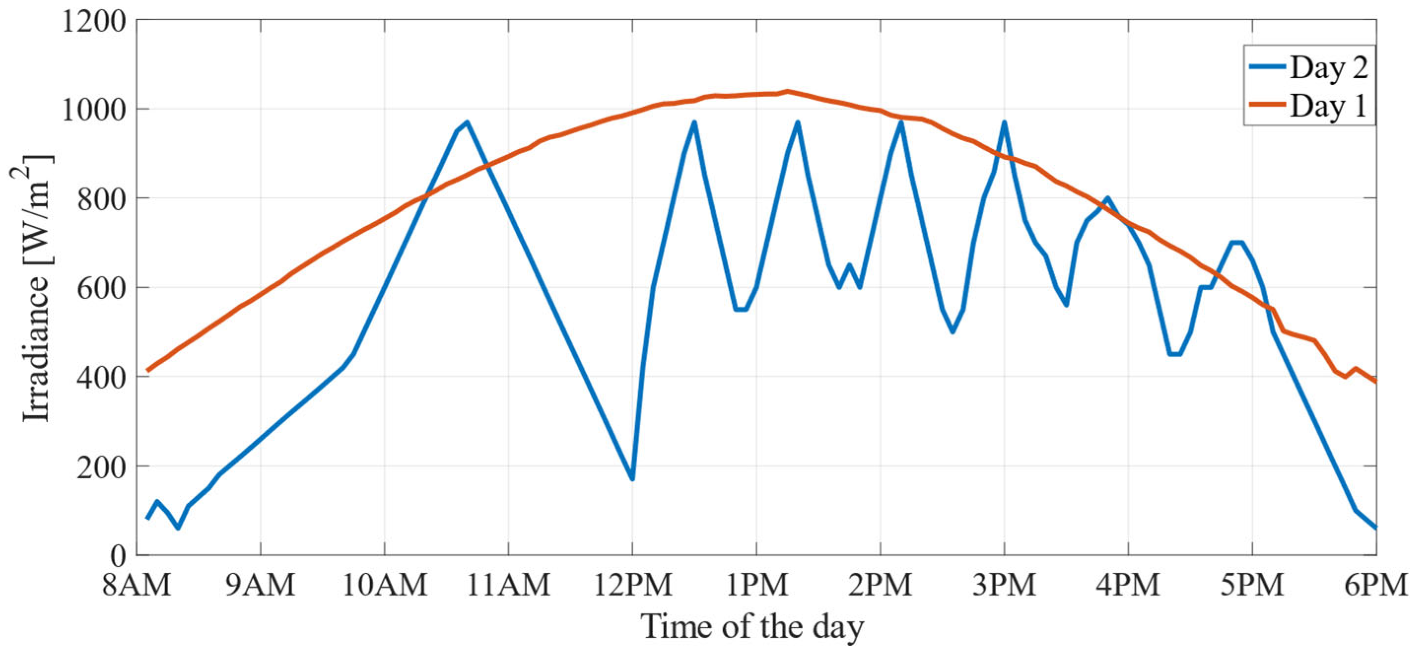
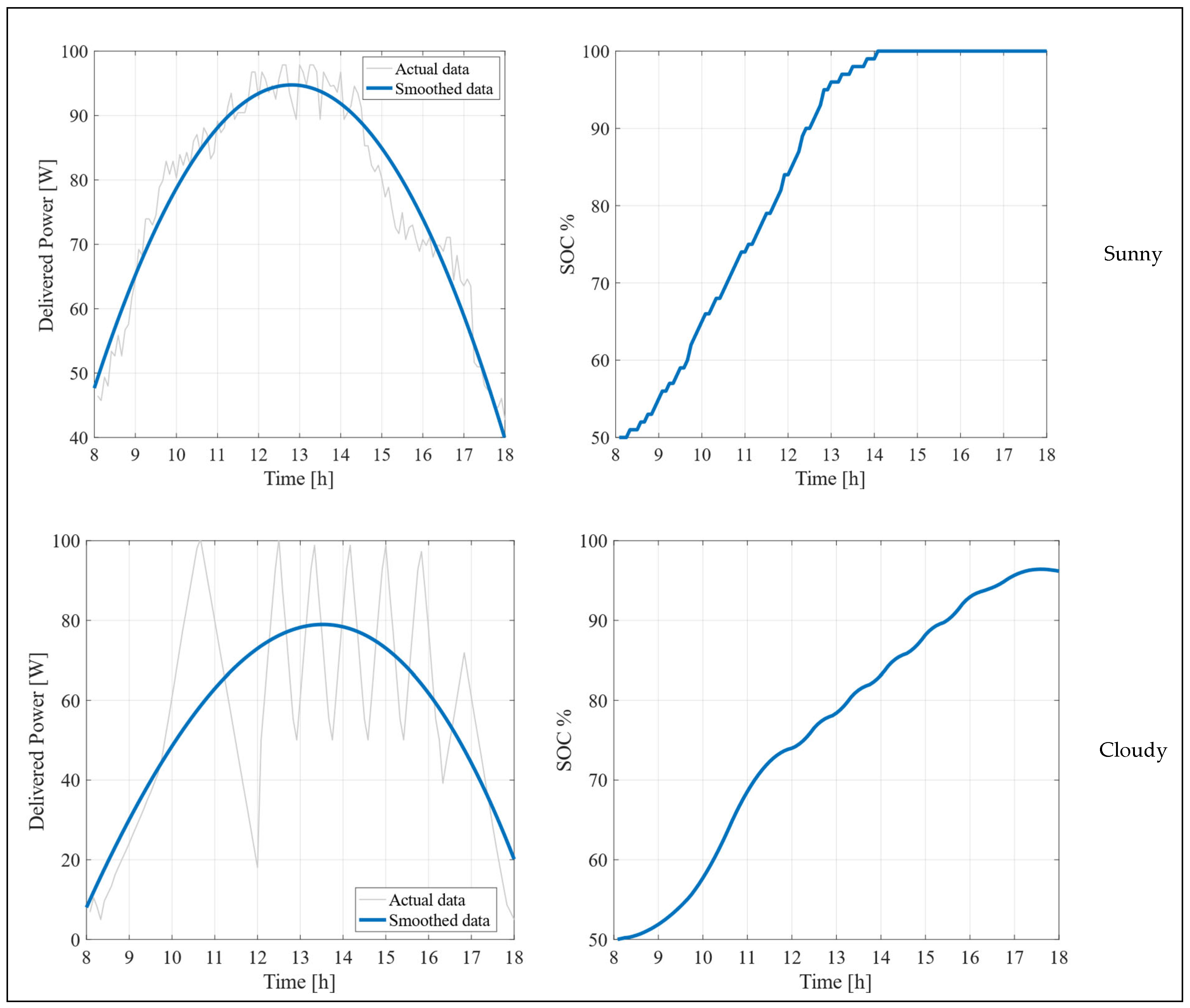
5.1. Experimental Results

All module setups recorded a maximum output power of around 95 W and fully charged their batteries in 6–7 h during the sunny day. However, measurable differences were observed between the different PV module setups in terms of delivered wattage and SOC between the sunny and cloudy days of the experiment. For instance, the flat module setup generated a maximum output power at 80 W, while the concave and convex module mounts recorded a maximum output power of 72 W and 65 W, respectively, on the cloudy day. None of the setups fully charged their designated batteries on that day as illustrated in Figure 5, Figure 6 and Figure 7. This suggests that curvature, especially convex shaping, introduces non-uniform irradiance and partial self-shading effects that compromise power generation efficiency. None of the modules reached full battery charge during the cloudy day, further emphasizing the importance of geometry in sub-optimal lighting.

These findings confirm that the geometry of flexible PV modules significantly affects performance in scattered light conditions, which are common in real-world situations. The quantitative differences between the flat and concave geometries (i.e., 18.75% decrease in peak power) and between the flat and convex geometries (i.e., 28.45% drop) show the impact that surface curvature has on the performance of photovoltaic modules. Moreover, the experimental data shows the need for predictive models to compensate for such performance. Future studies should expand the dataset to include a wider range of curvature radii and alternative geometries to better quantify these effects and improve model accuracies.

5.2. ML Models Results

A comparative analysis between all four models was conducted based on insights from their confusion matrices and calibration analysis.

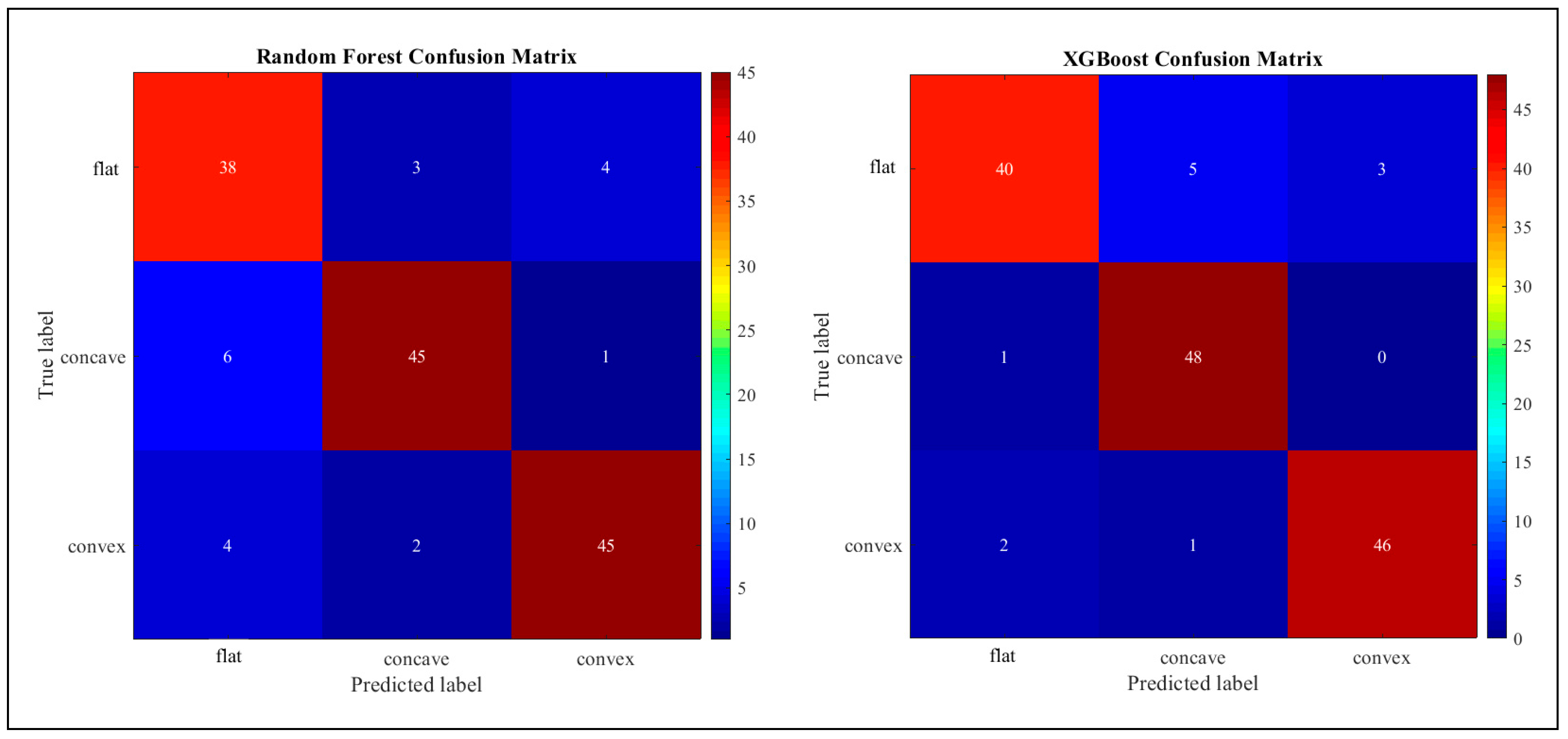
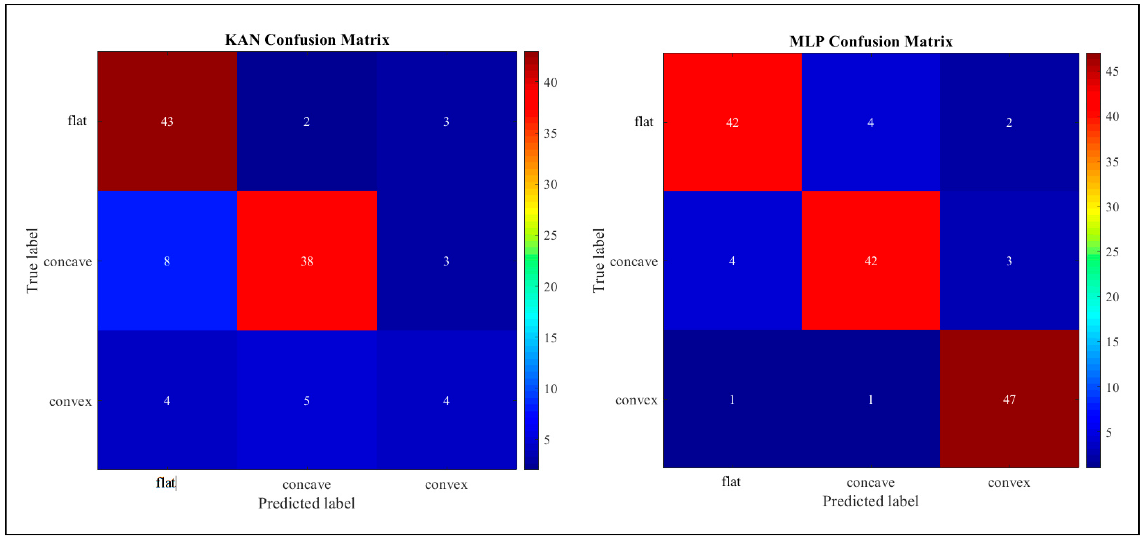
5.2.1. Confusion Matrix Insights

• The Random Forest (RF) classifier shows accurate results distinguishing between concave and convex PV modules with a recall of 90% but does not perform well with the flat module configuration, achieving 88% precision and 79% recall. This suggests that RF’s splitting criteria are more suitable with unique geometries.
• XGBoost achieved the best performance among all ML models, with 93% precision with the flat module and 98% recall with the unique module geometries.
• The Kolmogorov–Arnold Network (KAN) achieved a high recall of 90% with the flat PV module but a precision of only 78%, showing the false identification of curved modules’ instances. The KAN’s recall with the concave PV module was only 78%, showing some difficulty in identifying unique module geometries.
• The Multi-Layer Perceptron (MLP) showed 96% recall with the convex PV module and mediocre precision and recall with the other setups. Figure 8 illustrates the confusion matrices of all four deployed models.

Table 2. Output characteristics across all four ML models.

ML Model	Accuracy	Precision	Recall	F1-Score
RF	0.919 ± 0.016	0.921 ± 0.015	0.920 ± 0.016	0.919 ± 0.016
XGBoost	0.949 ± 0.014	0.950 ± 0.014	0.949 ± 0.014	0.949 ± 0.014
KAN	0.853 ± 0.022	0.860 ± 0.020	0.853 ± 0.022	0.852 ± 0.021
MLP 2	0.922 ± 0.020	0.924 ± 0.019	0.922 ± 0.021	0.922 ± 0.020

shows the accuracy, precision, and recall of the deployed ML models in this study. The table shows that across the four classifiers, XGBoost clearly leads with the highest mean accuracy, precision, recall, and F1 score, reflecting both its strong central tendency and low variance across folds. The MLP comes a close second indicating that a well-regularized deep network can nearly match gradient-boosted trees on this tabular task. RF trails slightly behind MLP, suggesting that while bagged trees handle nonlinearity robustly, they do not capture subtle feature interactions quite as effectively as XGBoost or the MLP. Finally, the KAN records the lowest scores, implying that its chaotic embedding benefits require further tuning or richer feature transforms to close the gap. Notably, XGBoost’s superior recall and precision consistency across classes underlines its overall dominance, whereas the larger standard deviation in the KAN underscores its sensitivity to hyperparameters. These patterns highlight that, for this balanced three-class problem, ensemble boosting remains the most reliable and interpretable choice, while neural architecture offer competitive alternatives with the right regularization and architecture search.

Figure 9 shows the macro-average ROC plot which shows that RF and XGBoost achieve virtually identical, near-perfect class separability with AUCs ≈ 0.99, with their curves hugging the top-left corner. The MLP trails only slightly, with an AUC of ≈0.98, indicating excellent but marginally lower discriminative power, particularly at very low false positive rates. In contrast, the KAN model exhibits a more gradual rise—with an AUC ≈ 0.95—reflecting that it requires a higher false positive rate to achieve the same true positive rates as the other models. Overall, the curves confirm that tree-based ensembles (RF, XGB) deliver the strongest class separation, the MLP is a close second, and the KAN, while still performing well above random, lags behind in its ability to rank positive instances with high confidence.

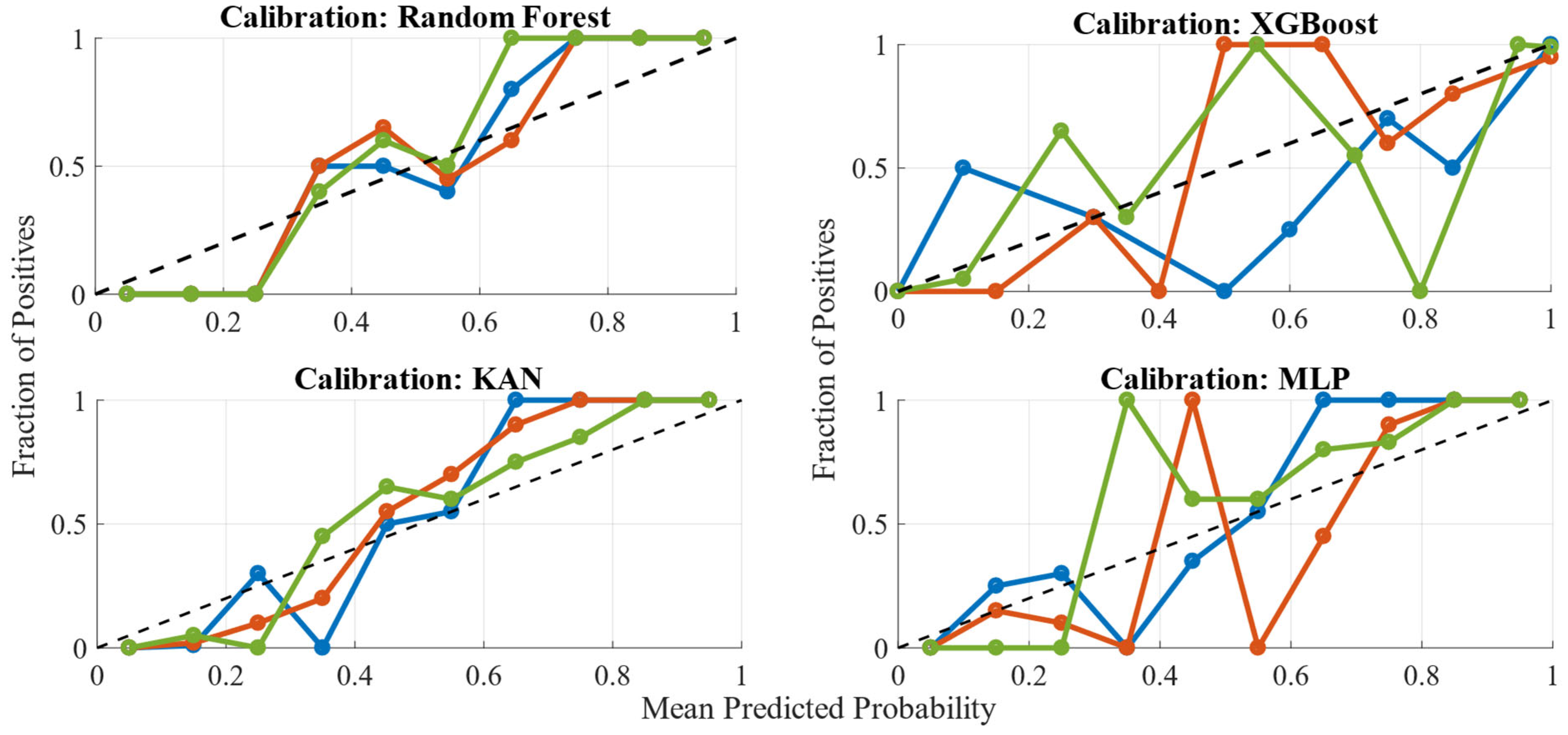
5.2.2. Calibration Analysis Across Models

A calibration curve (i.e., reliability diagram) is a way to check whether the probability of a deployed model matches real data scenarios. The calibration plots for Random Forest, XGBoost, the KAN, and the MLP show how well each prediction of the model aligns with the actual outcomes for the three PV module setups. A perfect line represents ideal calibration, where predicted probabilities match the actual observations, as shown in Figure 10.

The Random Forest (RF) and XGBoost models illustrated strong calibration with the flat PV module setup. However, they showed overconfidence with the concave and underconfidence with the convex panels. Consequently, RF shows prediction biases for curved shapes. Nonetheless, XGBoost was better calibrated than RF.

Furthermore, the KAN displayed a very different calibration result, showing improved calibration with the concave module compared with RF and XGBoost. However, the MLP model showed many calibration issues, resulting in severe underconfidence with the convex PV module. This made the MLP the least reliable of the four models.

5.2.3. Shapley Additive Explanations

Shapley Additive Explanations (SHAP) values are one way to explain the outputs of an ML method. Figure 11 shows the XGBoost SHAP beeswarm plot for the voltage feature, with the three horizontal bands representing the flat, concave, and convex PV modules with voltage values that are color-coded (i.e., red = high, blue = low). The top band represents the flat module while the middle and bottom bands represent the concave and convex modules, respectively. For the flat (top band) and convex (bottom band) modules, high voltages (red points) produce positive SHAP values, which makes prediction easier for these geometries. However, in the concave (middle band) module, high voltages lead to negative SHAP values, making concave predictions less likely.

6. Conclusions

In this study, four machine learning models were used to predict the geometry of flexible PV modules mounted in flat, concave, and convex configurations. Three identical 100 W, 2 mm thick modules were installed on adjustable mounts and connected to 12 V batteries via solar chargers. All modules reached full charge in 6–7 h on the sunny day, with a peak power output of 95 W. On the cloudy day, the concave and convex setups produced lower peak outputs of 72 W and 65 W, respectively. Among the ML models tested, XGBoost performed best, achieving 93% precision with the flat module and 98% recall with theshaped modules, while the KAN showed the lowest precision at 78% for the non-flat geometries. A calibration analysis showed that XGBoost and RF were well calibrated for flat modules but had overconfidence and underconfidence problems with the concave and convex modules, respectively. The KAN showed improved calibration for concave setups, and the MLP misclassified convex geometries.

Nevertheless, the presented results rely on limited data, harvested from two days of experiments. Expanding the dataset to cover different weather conditions could strengthen model accuracy. Future work will also explore different curvature radii (both concave and convex) and geometric configurations to deepen the understanding of the shape–performance relationship and further refine ML predictions for flexible PV technologies.

References

1. Renewables-2024. Available online: https://www.iea.org/reports/renewables-2024 (accessed on 20 March 2025).
2. IEA Report. 2025. Available online: https://www.iea.org/reports/net-zero-by-2050 (accessed on 20 March 2025).
3. Vodapally, S.N.; Ali, M.H. A Comprehensive Review of Solar Photovoltaic (PV) Technologies, Architecture, and Its Applications to Improved Efficiency. Energies 2023, 16, 319. [Google Scholar] [CrossRef]
4. Chung, J.; Kim, S.-W.; Li, Y.; Mariam, T.; Wang, X.; Rajakaruna, M.; Saeed, M.M.; Abudulimu, A.; Shin, S.S.; Guye, K.N.; et al. Engineering Perovskite Precursor Inks for Scalable Production of High-Efficiency Perovskite Photovoltaic Modules. Adv. Energy Mater. 2023, 13, 2300595. [Google Scholar] [CrossRef]
5. Manasrah, A.; Masoud, M.; Jaradat, Y.; Bevilacqua, P. Investigation of a Real-Time Dynamic Model for a PV Cooling System. Energies 2022, 15, 1836. [Google Scholar] [CrossRef]
6. Nezamisavojbolaghi, M.; Davodian, E.; Bouich, A.; Tlemçani, M.; Mesbahi, O.; Janeiro, F.M. The Impact of Dust Deposition on PV Panels’ Efficiency and Mitigation Solutions: Review Article. Energies 2023, 16, 8022. [Google Scholar] [CrossRef]
7. Manasrah, A.; Masoud, M.; Jaradat, Y.; Alia, M.; Almanasra, S.; Suwais, K. Shading Anomaly Detection Framework for Bi-Facial Photovoltaic Modules. Energy Sources Part Recovery Util. Environ. Eff. 2023, 45, 12955–12972. [Google Scholar] [CrossRef]
8. Wang, Z.; Wang, Y.; Zhang, X.; Yang, D.; Ma, D.; Ramakrishna, S.; Yuan, W.; Ye, T. Flexible Photovoltaic Micro-Power System Enabled with a Customized MPPT. Appl. Energy 2024, 367, 123425. [Google Scholar] [CrossRef]
9. Fukuda, K.; Sun, L.; Du, B.; Takakuwa, M.; Wang, J.; Someya, T.; Marsal, L.F.; Zhou, Y.; Chen, Y.; Chen, H.; et al. A Bending Test Protocol for Characterizing the Mechanical Performance of Flexible Photovoltaics. Nat. Energy 2024, 9, 1335–1343. [Google Scholar] [CrossRef]
10. Chen, Z.; Song, W.; Yu, K.; Ge, J.; Zhang, J.; Xie, L.; Peng, R.; Ge, Z. Small-Molecular Donor Guest Achieves Rigid 18.5% and Flexible 15.9% Efficiency Organic Photovoltaic via Fine-Tuning Microstructure Morphology. Joule 2021, 5, 2395–2407. [Google Scholar] [CrossRef]
11. Tian, X.; Wang, J.; Ji, J.; Xia, T. Comparative Performance Analysis of the Flexible Flat/Curved PV Modules with Changing Inclination Angles. Energy Convers. Manag. 2022, 274, 116472. [Google Scholar] [CrossRef]
12. Manasrah, A.; Al Zyoud, A.; Abdelhafez, E. Effect of Color and Nano Film Filters on the Performance of Solar Photovoltaic Module. Energy Sources Part Recovery Util. Environ. Eff. 2021, 43, 705–715. [Google Scholar] [CrossRef]
13. Rollo, A.; Settino, J.; Bevilacqua, P.; Ferraro, V. Influence of Different Photovoltaic Cooling Strategies on Its Average Monthly Performance. In Proceedings of the 2023 IEEE International Workshop on Metrology for Living Environment (MetroLivEnv), Milano, Italy, 29–31 May 2023; pp. 162–167. [Google Scholar]
14. Fatima, K.; Faiz Minai, A.; Malik, H.; García Márquez, F.P. Experimental Analysis of Dust Composition Impact on Photovoltaic Panel Performance: A Case Study. Sol. Energy 2024, 267, 112206. [Google Scholar] [CrossRef]
15. Oufettoul, H.; Lamdihine, N.; Motahhir, S.; Lamrini, N.; Abdelmoula, I.A.; Aniba, G. Comparative Performance Analysis of PV Module Positions in a Solar PV Array Under Partial Shading Conditions. IEEE Access 2023, 11, 12176–12194. [Google Scholar] [CrossRef]
16. Nicoletti, F.; Cucumo, M.A.; Ferraro, V.; Kaliakatsos, D.; Gigliotti, A. A Thermal Model to Estimate PV Electrical Power and Temperature Profile along Panel Thickness. Energies 2022, 15, 7577. [Google Scholar] [CrossRef]
17. Alcañiz, A.; Grzebyk, D.; Ziar, H.; Isabella, O. Trends and Gaps in Photovoltaic Power Forecasting with Machine Learning. Energy Rep. 2023, 9, 447–471. [Google Scholar] [CrossRef]
18. Al-Qawabah, S.M.; Abu Shaban, N.; Al Aboushi, A.; Al-Salaymeh, A.; Alma’aitah, A.; Abdelhafez, E. Prediction of the Output of the Tri-Generation Concentrated Solar Power System Based on Artificial Neural Network. In Proceedings of the 2024 6th Global Power, Energy and Communication Conference (GPECOM), Budapest, Hungry, 4 June 2024; pp. 345–349. [Google Scholar] [CrossRef]
19. Nicoletti, F.; Bevilacqua, P. Hourly Photovoltaic Production Prediction Using Numerical Weather Data and Neural Networks for Solar Energy Decision Support. Energies 2024, 17, 466. [Google Scholar] [CrossRef]
20. Output Power Prediction of a Photovoltaic Module Through Artificial Neural Network|IEEE Journals & Magazine|IEEE Xplore. Available online: https://ieeexplore.ieee.org/abstract/document/9926050 (accessed on 29 March 2025).
21. Alabdeli, H.; Rafi, S.; IG, N.; Rao, D.D.; Nagendar, Y. Photovoltaic Power Forecasting Using Support Vector Machine and Adaptive Learning Factor Ant Colony Optimization. In Proceedings of the 2024 Third International Conference on Distributed Computing and Electrical Circuits and Electronics (ICDCECE), Ballari, India, 26–27 April 2024; pp. 1–5. [Google Scholar]
22. Amiri, A.F.; Oudira, H.; Chouder, A.; Kichou, S. Faults Detection and Diagnosis of PV Systems Based on Machine Learning Approach Using Random Forest Classifier. Energy Convers. Manag. 2024, 301, 118076. [Google Scholar] [CrossRef]
23. Akhter, M.N.; Mekhilef, S.; Mokhlis, H.; Almohaimeed, Z.M.; Muhammad, M.A.; Khairuddin, A.S.M.; Akram, R.; Hussain, M.M. An Hour-Ahead PV Power Forecasting Method Based on an RNN-LSTM Model for Three Different PV Plants. Energies 2022, 15, 2243. [Google Scholar] [CrossRef]
24. Zhou, B.; Chen, X.; Li, G.; Gu, P.; Huang, J.; Yang, B. XGBoost–SFS and Double Nested Stacking Ensemble Model for Photovoltaic Power Forecasting under Variable Weather Conditions. Sustainability 2023, 15, 13146. [Google Scholar] [CrossRef]
25. Manasrah, A.; Masoud, M.; Jaradat, Y.; Jannoud, I. Advancements in Bifacial Photovoltaics: A Review of Machine Learning Techniques for Enhanced Performance. Eurasia Proc. Sci. Technol. Eng. Math. 2024, 27, 239–245. [Google Scholar] [CrossRef]
26. Yunqiao, L.; Yan, F. An Innovative Power Prediction Method for Bifacial PV Modules. Electr. Eng. 2023, 105, 2151–2159. [Google Scholar] [CrossRef]
27. Ghenai, C.; Ahmad, F.F.; Rejeb, O.; Bettayeb, M. Artificial Neural Networks for Power Output Forecasting from Bifacial Solar PV System with Enhanced Building Roof Surface Albedo. J. Build. Eng. 2022, 56, 104799. [Google Scholar] [CrossRef]
28. Kumar, B.S.; Kunar, B.M.; Murthy, C.S. Performance Evaluation and Machine Learning Analysis of 3 kW Grid-Connected Bifacial Solar Photovoltaic Systems. J. Inst. Eng. India Ser. B 2025. [Google Scholar] [CrossRef]
29. Mubarak, H.; Abdellatif, A.; Ahmad, S.; Hammoudeh, A.; Mekhilef, S.; Mokhlis, H. Prediction of Solar Photovoltaic Energy Output Based on Thin-Film Technology Utilizing Various Machine Learning Techniques. In Proceedings of the 2022 IEEE Global Conference on Computing, Power and Communication Technologies (GlobConPT), New Delhi, India, 23–25 September 2022; pp. 1–6. [Google Scholar]
30. Graditi, G.; Ferlito, S.; Adinolfi, G.; Tina, G.M.; Ventura, C. Energy Yield Estimation of Thin-Film Photovoltaic Plants by Using Physical Approach and Artificial Neural Networks. Sol. Energy 2016, 130, 232–243. [Google Scholar] [CrossRef]
31. Aslam, M.; Lee, J.-M.; Hong, S. A Multi-Layer Perceptron Based Deep Learning Model to Quantify the Energy Potentials of a Thin Film a-Si PV System. Energy Rep. 2020, 6, 1331–1336. [Google Scholar] [CrossRef]
32. Akhter, M.N.; Mekhilef, S.; Mokhlis, H.; Ali, R.; Usama, M.; Muhammad, M.A.; Khairuddin, A.S.M. A Hybrid Deep Learning Method for an Hour Ahead Power Output Forecasting of Three Different Photovoltaic Systems. Appl. Energy 2022, 307, 118185. [Google Scholar] [CrossRef]
33. Kurz, D.; Morawska, L.; Piechota, R.; Trzmiel, G. Analysis of the Impact of a Flexible Photovoltaic Tile Shape on Its Performance. E3S Web Conf. 2018, 44, 00085. [Google Scholar] [CrossRef]
34. Bednar, N.; Caviasca, A.; Sevela, P.; Severino, N.; Adamovic, N. Modelling of Flexible Thin-Film Modules for Building and Product Integrated Photovoltaics. Sol. Energy Mater. Sol. Cells 2018, 181, 38–45. [Google Scholar] [CrossRef]
35. Du, D.; Qiao, F.; Guo, Y.; Wang, F.; Wang, L.; Gao, C.; Zhang, D.; Liang, J.; Xu, Z.; Shen, W.; et al. Photovoltaic Performance of Flexible Perovskite Solar Cells under Bending State. Sol. Energy 2022, 245, 146–152. [Google Scholar] [CrossRef]
36. Dong, Q.; Chen, M.; Liu, Y.; Eickemeyer, F.T.; Zhao, W.; Dai, Z.; Yin, Y.; Jiang, C.; Feng, J.; Jin, S.; et al. Flexible Perovskite Solar Cells with Simultaneously Improved Efficiency, Operational Stability, and Mechanical Reliability. Joule 2021, 5, 1587–1601. [Google Scholar] [CrossRef]
37. Kumar, D.D.S.; Agrawal, D.M.; Kasulla, M.S.; Kumar, D.A. A Textbook on Fundamentals of Renewable Energy and Green Technology; Academic Guru Publishing House: Bhopal, India, 2024; ISBN 978-81-973048-4-2. [Google Scholar]
38. Akiba, T.; Sano, S.; Yanase, T.; Ohta, T.; Koyama, M. Optuna: A Next-Generation Hyperparameter Optimization Framework. In Proceedings of the 25th ACM SIGKDD International Conference on Knowledge Discovery & Data Mining, Anchorage, AK, USA, 4–8 August 2019; Association for Computing Machinery: New York, NY, USA, 2019; pp. 2623–2631. [Google Scholar]
Figure 1. Schematics of the concave and convex geometries of the PV modules, showing angles of sunlight at different times of the day. (Note: shapes in the figure are exaggerated and not to scale).
Energies 18 03529 g001
Figure 2. The adjustable contraption setup on which the flexible PV modules were mounted.
Energies 18 03529 g002
Figure 3. Recorded sunlight radiation during day 1 (sunny) and day 2 (cloudy) in W/m2.
Energies 18 03529 g003
Figure 4. Simulation pipeline flowchart of proposed ML methods.
Energies 18 03529 g004
Figure 5. Output power and SOC of the flat-mounted PV module during sunny and cloudy days.
Energies 18 03529 g005
Figure 6. Output power and SOC of the concavely mounted PV module during sunny and cloudy days.
Energies 18 03529 g006aEnergies 18 03529 g006b
Figure 7. Output power and SOC of the convexly mounted PV module during sunny and cloudy days.
Energies 18 03529 g007aEnergies 18 03529 g007b
Figure 8. Confusion matrices for all four deployed ML models.
Energies 18 03529 g008aEnergies 18 03529 g008b
Figure 9. Macro-Average ROC for all four deployed ML models.
Energies 18 03529 g009
Figure 10. Calibration curves for all four deployed ML models showing flat (blue), concave (red), and convex (green) modules against an ideal calibration (dashed line).
Energies 18 03529 g010
Figure 11. Shapley Additive Explanations (SHAP) voltage values for the flat (top band), concave (middle band), and convex (bottom band) modules.
Energies 18 03529 g011