A Spatio-Temporal Microsimulation Framework for Charging Impact Analysis of Electric Vehicles in Residential Areas: Sensitivity Analysis and Benefits of Model Complexity

Abstract

The increasing share of electric vehicles (EVs) offers many advantages, including a reduced CO₂ footprint over the vehicles’ lifetime and improved resource efficiency through the recycling of high-voltage batteries. At the same time, the growing EV share presents challenges, such as ensuring sufficient power supply for the simultaneous charging of EVs within existing distribution grids. The scientific community has conducted numerous studies on the interaction between EVs and distribution grids, employing increasingly complex modeling techniques. However, the benefits of more complex modeling are rarely quantified. This study aims to address this gap by evaluating the impact of modeling complexity on transformer peak loads and busbar voltage for three communities with real-world distribution grid data. Since numerous stochastic factors influence EV charging patterns, this paper introduces a modular framework that accounts for the interconnection of these factors through microsimulation. The framework models charging events of battery electric vehicles (BEVs) and comprises modules for synthetic population generation, weekly mobility pattern assignment, and energy demand modeling based on vehicle class and ambient conditions. The findings reveal that cost-optimized charging strategies and seasonal factors, such as cold weather, have a significantly greater impact on the distribution grid than the detailed modeling of sociodemographic mobility patterns or detailed modeling of a diversified vehicle fleet.

1. Introduction

The growing share of electric vehicles (EVs) holds significant potential to enable emission-free mobility. With the continued decarbonization of energy production and consistent implementation of material recycling, EVs could reduce environmental impacts in 2050 to one-third of the levels of gasoline-powered vehicles in fundamental impact categories, such as global warming potential, cumulative energy demand, and acidification potential [1]. To support this transition, it is essential to identify and address potential challenges early on. Among the key challenges is the impact of EV charging on the electricity grid, particularly on distribution grids, as up to 80% of charging sessions are expected to occur at home, where simultaneous charging could strain grid capacity [2]. The scientific literature suggests several mitigation strategies, including indirect control of EV charging through time-of-use (TOU) pricing, smart charging schemes, and infrastructural upgrades [3]. However, when the share of electric vehicles reaches critical levels, grid reinforcements may become necessary, potentially leading to high costs and long lead times. In this context, an accurate modeling and impact analysis of EV charging on distribution grids is crucial. Clement-Nyns et al. were among the first to apply statistical modeling to assess the impact of EV charging on distribution grids in 2010 [4]. Their study focused on minimizing power losses during EV charging while adhering to grid constraints. Mobility behavior was represented using probabilistic methods, and synthetic distribution grids were employed for analysis. The first studies incorporating more detailed representations of mobility were conducted by Galus et al. [5] and Waraich et al. [6]. These works utilized agent-based transportation models based on the activity chains of individual vehicle users, thereby establishing a bottom-up modeling approach that combined methodologies from both transportation research and power systems engineering to enhance the overall level of detail. In the following years, a range of studies introduced further refinements. For example, Gschwendtner et al. [7] modeled the plug-in behavior of EV users, while Fischer et al. [8] explored the influence of socio-economic attributes on charging behavior. However, despite the increasing level of detail in mobility, plug-in behavior, and charging models, the added value of growing model complexity has received limited attention. Addressing this specific research gap is the focus of the present study. The first studies explicitly investigating this area were conducted by Stiasny et al. [9] and Karmaker et al. [10]. Stiasny et al. performed a sensitivity analysis for a real municipality, examining the impact of varying modeling parameters on transformer peak load and line loadings. However, impact on busbar voltage was not considered. Although different mobility models were tested, mobility profiles were not assigned based on sociodemographic characteristics. Instead, they were randomly sampled from statistical distributions and randomly allocated to households. Karmaker et al. presented a case study for a municipality in Australia, where mobility was modeled using stochastic parameters such as daily driving distance. However, it remains unclear how a detailed microscopic modeling approach that links mobility to sociodemographic characteristics influences distribution grid impact analysis.

While both studies provide valuable sensitivity analyses and identify key parameters affecting distribution grid impact, three critical aspects remain unaddressed:

• First, neither study evaluates the impact of modeling a synthetic population with mobility patterns explicitly tied to sociodemographic attributes. Instead, mobility profiles are assigned independently of these factors, relying solely on stochastic sampling and random allocation. This risks overlooking systematic behavioral differences between user groups that could significantly affect results. Although the importance of sociodemographic profiling in mobility modeling is increasingly recognized, its specific impact on distribution grid assessments remains insufficiently explored.
• Second, both studies focus only on transformer peak loads and line loadings, although busbar voltage violations often occur earlier and pose a great risk to system stability [11,12]. Busbar voltage violations occur when local voltages at distribution grid busbars fall below thresholds defined by standards such as EN 50160 [13]. Due to the spatial variability and strong dependence on local grid topology, busbar voltages are likely far more sensitive to localized changes introduced by detailed modeling than aggregated transformer loads or line loadings. Therefore, capturing sensitivities in busbar voltages requires a more detailed, spatially resolved modeling approach.
• Third, both studies apply sensitivity analyses to only a single distribution grid, making it difficult to assess variability across different real-world distribution grids. This study addresses this limitation by analyzing three real-world municipalities, allowing for an assessment of the consistency of observed trends across different grid topologies.

This study addresses these gaps by conducting sensitivity analyses across seven scenarios with varying model complexities. It incorporates a synthetic population with sociodemographically assigned mobility patterns and evaluates impacts on both transformer peak loads and busbar voltages in three real-world distribution grids. The most influential factors identified are then used to assess grid impacts under varying EV penetration levels. All analyses are performed using a modular simulation framework that allows for the flexible substitution of individual model components with simpler or more detailed alternatives. This work makes the following contributions:

• The introduction of the modular simulation framework with a bottom-up modeling approach.
• The modeling of three communities in the suburbs of Stuttgart using real distribution grid data.
• The creation of a synthetic, representative population based on census and microcensus data with a spatial resolution of 100 m × 100 m.
• The modeling of the synthetic population’s mobility behavior using MOP data.
• The modeling of household baseload and a representative, diversified vehicle fleet of BEVs.
• A sensitivity analysis of seven EV charging scenarios, focusing on the impact of model complexity on transformer peak load and busbar voltage for each of the three communities.
• The identification of key impact parameters that most significantly affect transformer peak load and busbar voltage.
• A stochastic load flow simulation considering the identified key impact parameters under varying EV penetration rates for each of the three communities.

2. Materials and Methods

The impact of EV charging on distribution grids is analyzed using a modular simulation framework. Each module functions as an independent building block that can be replaced with either simplified or more detailed modeling approaches, depending on the availability and resolution of input data. Figure 1 shows an overview of the framework’s module structure. The modules are represented by boxes and the data sources by storage symbols. The simulation framework includes the following modules:

• Population Synthesis Module: Creates a virtual population that closely resembles the actual population. The synthesized population is assigned to buildings, which are connected to the distribution grid.
• Grid Module: Provides distribution grid data from three real-world distribution grids in the suburbs of Stuttgart.
• Mobility Pattern Module: Models the weekly mobility behavior of household residents using MOP data. Since electric vehicle charging does not always occur daily, analyzing continuous weekly mobility patterns provides valuable insights [14].
• Vehicle Fleet Module: Assigns representative vehicles to households. The vehicle parameters depend on real-world data from an electric vehicle database [15].
• Charging Price Module: Provides EEX day-ahead AC charging prices for cost optimized charging strategies.
• Household Loadprofile Module: Assigns annual household baseload profiles with a 15 min resolution. The annual consumption is scaled based on household size.
• Charging Strategy Module: Enables the modeling of different charging strategies.
• Charging Optimization Module: Implements charging plan optimization using the Pyomo optimization framework [16,17] with the SCIP solver [18].
• Power Flow Computation Module: Performs power flow calculations using Pandapower [19].

The simulation framework is designed for Germany but can be easily transferred to other countries. For this, only the population synthesis and mobility pattern modules need to be adapted based on data availability. Different local penetration rates and charging strategies, including the maximum possible charging power, are already accounted for in the proposed modules. The required adjustments are described in the following module subchapters.

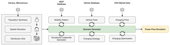
Figure 1. Simulation framework with interchangeable modules. The modularity enables substitution based on targeted modeling complexity and data availability.

Figure 1. Simulation framework with interchangeable modules. The modularity enables substitution based on targeted modeling complexity and data availability.

2.1. Population Synthesis Module

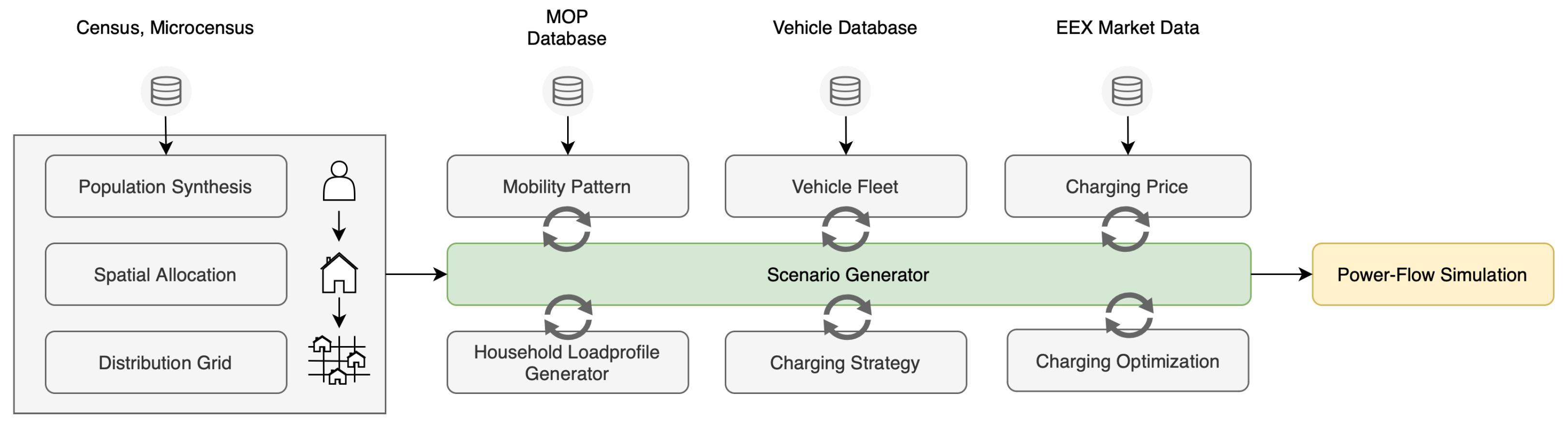
The population synthesis module generates a synthetic population for a community, ensuring that household and person attributes, as well as their spatial distribution in buildings, closely reflect the actual population. A realistic synthetic population is important for two reasons. First, the sociodemographic structure of households influences mobility behavior, which can impact EV charging patterns. Second, the spatial distribution of households across different building units can affect power flow calculations, as a uniform distribution fails to capture the clustering of households in multi-family homes. In this study, the synthetic population is generated to match the distributions of household and population attributes, including household size, age, and income, across two geographic levels: Level 1: municipality level; Level 2: 100 m × 100 m spatial grid level. The population synthesis unfolds in three stages:

• The harmonization of household and population attributes across both geographic levels. Due to privacy restrictions, some household and population attributes in sparsely populated 100 m × 100 m grid cells are slightly modified by the data-providing government agency. To correct these modifications and ensure that the sum across all grid cells matches the municipality-level marginals, a manual harmonization approach is applied. Feasible replacement cells are constructed with minimal adjustments to the attributes, and a simulated annealing algorithm is used to assign these replacements while minimizing both the number of altered cells and the extent of modification.
• An iterative proportional updating (IPU) of household and population attributes.
• The spatial allocation of households to building units connected to the distribution grid.

The data sources for the household and person attributes in this study are the 2011 Census [20] and the 2011 Microcensus Scientific Use File (SUF) [21] of Germany. The Microcensus SUF provides a de facto anonymized 70% subsample of the 2011 Microcensus. While the 2011 Census data is publicly accessible, federal and state statistical offices provide the Microcensus Scientific Use File for a fee to domestic research institutions. The modeling approach is directly transferable to other countries, provided that household and population data is available at both geographic levels. If data at the 100 m × 100 m level is unavailable, households can be randomly assigned or spatially distributed based on the identification of multi-family buildings using geoinformation systems.

2.1.1. Household and Population Attribute Harmonization

Stage one involves extracting marginal values for household and population attributes from the 2011 census [20]. Data from two spatial resolutions is utilized to create a realistic spatial distribution of households across building units: the regional level, representing the entire municipality, and the 100 m × 100 m grid cell level. Table 1 provides an overview of the household and population marginals used in the population synthesis, indicating their availability at both the municipal and 100 m × 100 m grid level. While municipal-level marginals closely align with actual distributions, those at the 100 m × 100 m grid level may deviate slightly, particularly in grid cells with very few households. This deviation is caused by the SAFE method, a statistical privacy protection measure used in the 2011 census to protect participants’ privacy [22]. To address this deviation, a harmonization method is applied to align attributes between the 100 m × 100 m grid cells and the municipal level. For grid cells containing fewer than three households, a set of alternative cells with slightly adjusted attributes is generated. This is followed by a simulated annealing approach where the original cells are replaced with their alternatives. This process continues until the aggregated household and population attributes at the 100 m × 100 m grid level align with those at the municipal level. This approach ensures a minimal adjustment in the raw census data while achieving full harmonization of household and population attributes across both spatial resolutions. Simulated annealing is a heuristic optimization technique known for its ability to escape local optima with a certain probability [23]. This capability is particularly advantageous given the vast number of possible alternative cells and the likelihood of encountering numerous local minima during the harmonization process. Mathematically, the simulated annealing method is represented by Equations (1) and (2).

Equation (1) introduces an L1 distance measure $E^{*}$ to capture the attribute difference between the municipal level and the aggregated 100 m × 100 m level data. $s_0$ represents the initial state of the cells, while $s^{*}$ describes the initial state altered by alternative cells. The distance measure consists of two terms. Term 1 prioritizes attributes at the municipal level by assigning them greater weight in the L1 distance measure. These include, for example, the number of households or the population count. Thus, the weighted distance between a selection of aggregated cell attributes $s_i^{*}$ and a selection of municipal attributes ${\psi }_i$ is modeled through the weighting variable ${\lambda }_i$. Term 2 measures the L1 distance between the initial state $s_0$ and the altered state $s^{*}$.

Equation (2) outlines the selection process for $s^{*}$ using the simulated annealing method. The alternative state $s^{*}$ is always accepted if its associated distance measure $E^{*}$ is smaller than the initial distance E, representing the unaltered 100 m × 100 m cells. However, $s^{*}$ may also be accepted with a certain probability, even if $E^{*}\ge E$, enabling the algorithm to escape local minima. This probability decreases progressively over iterations and is governed by the parameter T, representing a monotonically decreasing sequence of positive values. Once the attribute distance $E^{*}$ converges, the household and population attributes are fully harmonized across both spatial resolutions.

$$E^{*}=\sum _i{\lambda }_i\left|s_i^{*}-{\psi }_i\right|+\left|s^{*}-s_0\right|$$

(1)

$$P(E,E^{*},T)=\left\{\begin{array}{cc}1\hfill & \mathrm{if}{E}^{*}<E\hfill \\ exp\left(-{\displaystyle \frac{E^{*}-E}{T}}\right)\hfill & \mathrm{if}\mathrm{else}\hfill \end{array}\right.$$

(2)

Table 1. Utilized household and person marginal attributes on municipality and 100 m × 100 m grid level for population synthesis.

Type	Attribute	Characteristic	Geo-Resolution
Household	Total Number	Sum	Municipality, Grid
	Size	1, 2, 3, 4, 5, 6+	Municipality, Grid
	Net Income	5 Groups	Municipality
Person	Total Number	Sum	Municipality, Grid
	Gender	[m, f]	Municipality, Grid
	Age	9 Groups	Municipality, Grid
	Gender × Age	[m, f] × [9 Groups]	Municipality
	Employed	yes, no	Municipality

Table 1. Utilized household and person marginal attributes on municipality and 100 m × 100 m grid level for population synthesis.

Type	Attribute	Characteristic	Geo-Resolution
Household	Total Number	Sum	Municipality, Grid
	Size	1, 2, 3, 4, 5, 6+	Municipality, Grid
	Net Income	5 Groups	Municipality
Person	Total Number	Sum	Municipality, Grid
	Gender	[m, f]	Municipality, Grid
	Age	9 Groups	Municipality, Grid
	Gender × Age	[m, f] × [9 Groups]	Municipality
	Employed	yes, no	Municipality

2.1.2. Iterative Proportional Updating (IPU)

To create a representative population, households with corresponding persons are drawn from the 2011 Microcensus Scientific Use File (SUF) [21]. The 2011 Microcensus is an anonymized area sample comprising approximately 7.9 million people living in private households and communal accommodations across primary and secondary residences in Germany. The Scientific Use File represents a de facto anonymized 70% subsample of the 2011 Microcensus. The microcensus data provides detailed, disaggregated information on households and individuals but lacks precise spatial resolution, available only at the federal-state level. To allocate disaggregated households from the microcensus to the 100 m × 100 m grid cells, microcensus attributes must be aligned with the two geographical levels. A mathematical method that enables such a reconstruction is iterative proportional fitting (IPF). The initial work on this method dates back to 1940, when Deming et al. introduced an approach using a least-squares procedure to adjust frequency tables such that they fit expected marginals [24]. This method is not applied in this study as it does not support the simultaneous fitting of household and population attributes across multiple geographic resolutions. Instead, the iterative proportional updating (IPU) method by Konduri et al. [25] is employed, which extends the method of Ye et al. [26] by enabling fitting across two geographical levels. The two geographic levels considered are the municipality and the 100 m × 100 m grid level. The attributes used in the IPU process are listed in Table 1. Once the IPU procedure converges, representative households are sampled from the microcensus using the adjusted weights and allocated to the 100 m × 100 m grid cells. Figure 2 illustrates the three-step population synthesis process: population and household attribute harmonization, followed by iterative proportional updating and spatial household allocation.

Figure 2. Three-stage population synthesis process. Stage 1: Household and population data gathering from census with harmonization of household and population attributes across two spatial resolutions: municipality level and 100 m × 100 m grid level. Stage 2: Iterative proportional updating (IPU) with sample weight updating and drawing from microcensus. Stage 3: Spatial allocation of households.

Figure 2. Three-stage population synthesis process. Stage 1: Household and population data gathering from census with harmonization of household and population attributes across two spatial resolutions: municipality level and 100 m × 100 m grid level. Stage 2: Iterative proportional updating (IPU) with sample weight updating and drawing from microcensus. Stage 3: Spatial allocation of households.

2.1.3. Spatial Household Allocation

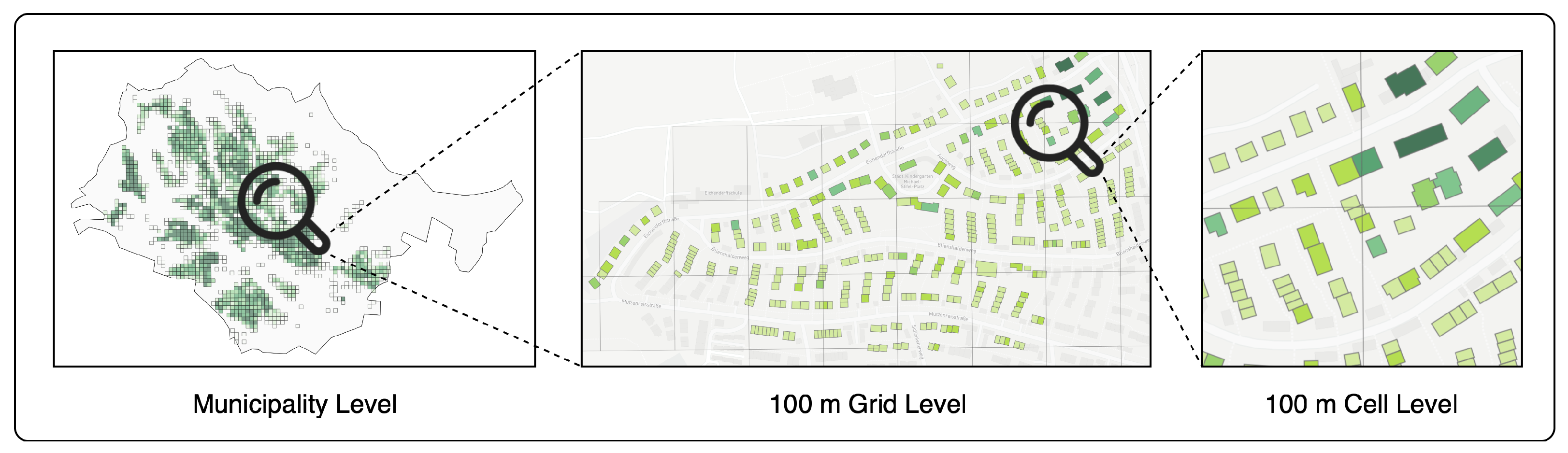
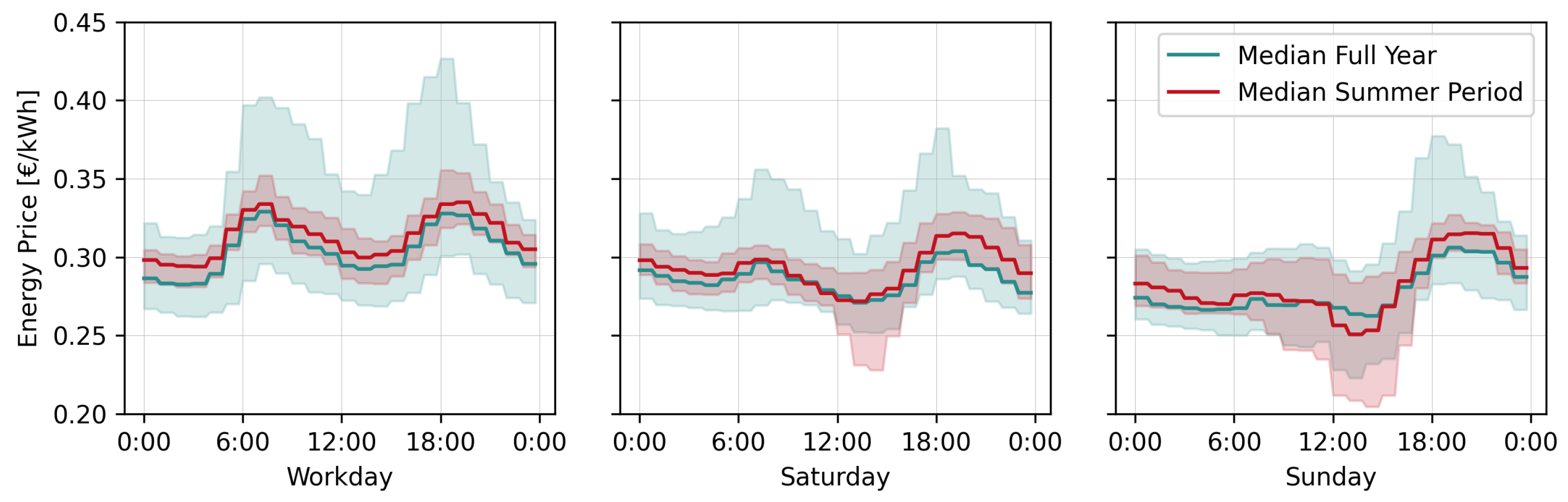
After generating the synthetic population for the 100 m × 100 m grid, the next step is to assign households to building units. A simplified approach, such as uniformly distributing households across buildings, would fail to capture local clustering effects. To address this, a modeling approach that incorporates geoinformation system (GIS) analysis is employed. This analysis identifies the building footprint and building type. The likelihood of assigning multiple households to a building increases with the footprint size and classification as a multi-family building. Figure 3 provides an example of a fully generated and spatially distributed synthetic population for a municipality across three zoom levels: Level 1: municipality level; Level 2: 100 m × 100 m grid level; Level 3: magnified 100 m × 100 m grid level, showing individual building units. Darker shades of green indicate a higher number of assigned households.

Figure 3. Example of a fully generated and spatially distributed synthetic population for a municipality across 3 zoom levels. Level 1: municipality level. Level 2: 100 m × 100 m grid level. Level 3: magnified 100 m × 100 m grid level, showing individual building units. Darker shades of green indicate a higher number of assigned households.

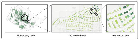
Figure 3. Example of a fully generated and spatially distributed synthetic population for a municipality across 3 zoom levels. Level 1: municipality level. Level 2: 100 m × 100 m grid level. Level 3: magnified 100 m × 100 m grid level, showing individual building units. Darker shades of green indicate a higher number of assigned households.

2.2. Mobility Module

To model EV charging events, mobility profiles must be assigned to the synthetic population. For Germany, two datasets are suitable for this purpose:

Mobility in Germany (MiD): This dataset is based on a nationwide survey of representative households regarding their daily travel behavior. It is conducted on behalf of the Federal Ministry for Digital and Transport and provides cross-sectional data, capturing everyday mobility on a specific reference day [27].

German Mobility Panel (MOP): The MOP is a longitudinal survey with representative households. All household individuals aged ten and older complete a travel diary, documenting their mobility over a full week [14].

This study uses the MOP datasets from 2011 to 2018, as they are better suited for modeling vehicle availability for charging over a full week, whereas the MiD data covers only a single day and cannot capture weekly variations. The datasets are filtered to include only regions with high urbanization or dense populations, ensuring a more accurate representation of the suburban area around Stuttgart. The MOP data is assigned to the synthetic population by matching household size and household type attributes, as shown in Figure 4. The household size attribute is available in both the synthetic population and the MOP dataset. The MOP dataset classifies households into four types, whereas the synthetic population does not directly use the same categories. However, a transformation is straightforward since all the required attributes are available in the synthetic population dataset. The limitation to two attributes is deliberately chosen to avoid overly restricting the pool of eligible households, which would compromise the stochastic nature of the modeling. Since multiple MOP records match a given household size and type, Monte Carlo sampling is used to randomly select one record. A separate assignment of the number of household vehicles is not necessary since the MOP household dataset already includes the number of vehicles per household. However, an additional modeling step is required to derive a vehicle usage profile from the mobility profile, as the MOP dataset does not provide a direct mapping of household members to vehicles. This is implemented by assigning the vehicle with the largest battery capacity to the household member with the highest daily mileage. Vehicles are considered available only if they are not in use by another household member and are located at the starting point of the trip. Although the MOP data includes the number of vehicles per household, it does not provide details such as specific vehicle models. These attributes are assigned separately via the vehicle module.

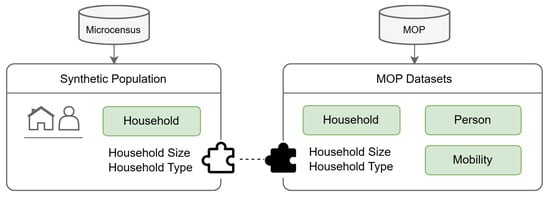
Figure 4. Assignment of MOP data to synthetic populations households. Matching criteria are household size and household type.

Figure 4. Assignment of MOP data to synthetic populations households. Matching criteria are household size and household type.

Table 2 presents the average vehicle travel distance for MOP household types 1–4 on workdays, Saturdays, and Sundays. Notably, household type 2, consisting of non-employed or retired individuals, exhibits significantly lower travel distances on workdays than other household types, likely affecting vehicle energy demand.

Figure 5 shows the probability density of home arrival times for household types 1–4 throughout the week. While household types 1, 3, and 4 share similar probability distributions, household type 2 exhibits a distinct midday arrival peak, whereas the other types display the typical evening peak. This suggests that incorporating household type attributes into a detailed mobility model could yield different results if the share of retired individuals deviates significantly from the MOP proportions shown in Table 3. Transferring the mobility module to other countries requires assigning mobility profiles based on the available sociodemographic attributes. If household types are not available in a form comparable to the four types in the MOP dataset, efforts should at least be made to collect data on the number of retired or unemployed persons on the municipality level. Separate mobility profiles should then be assigned to these individuals, as their mobility behavior differs most significantly from the rest of the population.

Table 2. Average vehicle travel distance for MOP household types 1–4 for workdays, Saturdays, and Sundays. Data source: MOP datasets from 2011 to 2018.

Household Type	Vehicle Average Travel Distance [km]
	Workday	Saturday	Sunday
1	35.0	28.6	25.6
2	17.8	19.0	18.3
3	25.7	18.6	17.3
4	28.5	23.8	22.7

Table 2. Average vehicle travel distance for MOP household types 1–4 for workdays, Saturdays, and Sundays. Data source: MOP datasets from 2011 to 2018.

Household Type	Vehicle Average Travel Distance [km]
	Workday	Saturday	Sunday
1	35.0	28.6	25.6
2	17.8	19.0	18.3
3	25.7	18.6	17.3
4	28.5	23.8	22.7

Table 3. MOP household types with their characteristics and relative share in the MOP dataset from 2011 to 2018.

Household Type	Characteristics	Relative Share [%]
1	1–2 employed persons.	43.1
2	1–2 non-employed (retired) persons.	37.3
3	Household with children below 18 years.	15.3
4	Household w/o children. 3+ persons.	4.3

Table 3. MOP household types with their characteristics and relative share in the MOP dataset from 2011 to 2018.

Household Type	Characteristics	Relative Share [%]
1	1–2 employed persons.	43.1
2	1–2 non-employed (retired) persons.	37.3
3	Household with children below 18 years.	15.3
4	Household w/o children. 3+ persons.	4.3

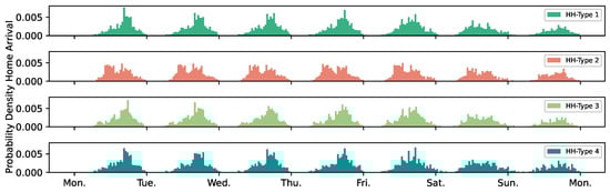
Figure 5. Probability density home arrival for MOP household types 1–4 over the course of one week. Data source: MOP datasets from 2011 to 2018.

Figure 5. Probability density home arrival for MOP household types 1–4 over the course of one week. Data source: MOP datasets from 2011 to 2018.

2.3. Household Loadprofile Module

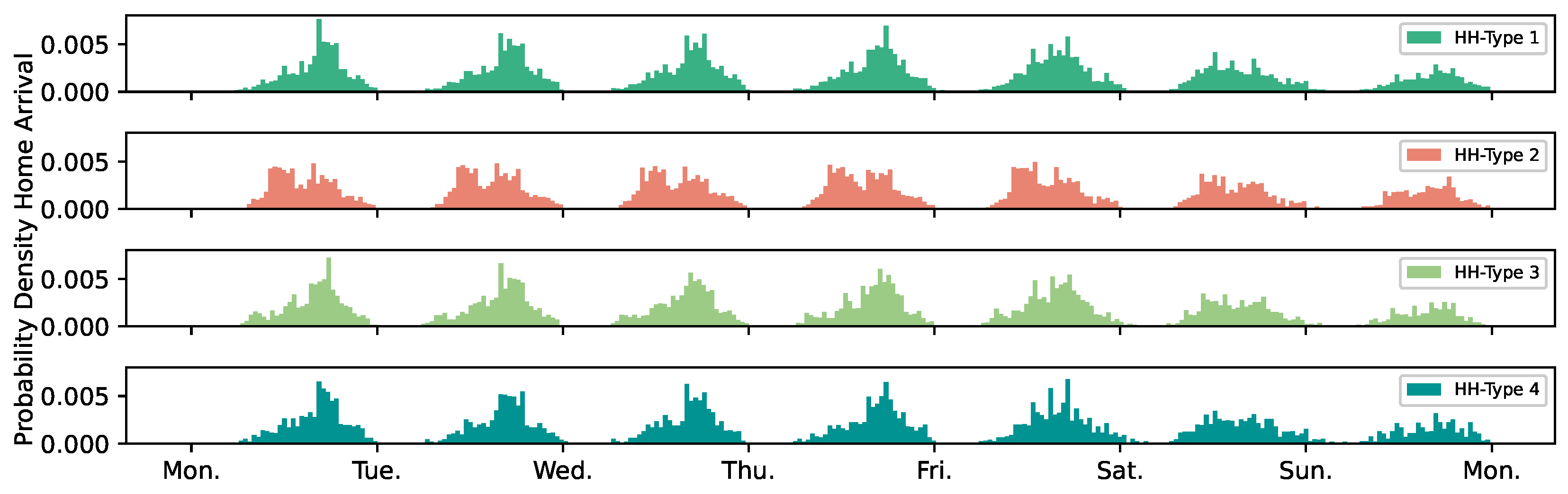
Synthetic household load profiles are generated using a load profile generator developed by Uhrig et al. [28]. This tool produces annual household consumption profiles with a 15 min resolution based on a validated measurement campaign. All profiles are normalized and then scaled to match the average annual consumption for each household size, using data from [29]. Finally, the load profiles are randomly assigned to households according to their size classification. Figure 6 illustrates an example of an aggregated, averaged household load profile for one of the three municipalities analyzed in this study. This municipality includes approximately 465 households connected to the distribution grid. The chart displays the average load profile for both the summer season (15 May–14 September) and the winter season (1 November–20 March). The shape of the curves aligns well with the H0 standard load profile (SLP) [30]. For validation, the average annual household consumption is calculated for each of the three municipalities, with values ranging from 3200 to 3400 kWh. This range is consistent with multi-year figures published by the Federal Statistical Office [29].

Figure 6. Aggregated average household load profile for a community of 465 households with varying household sizes, covering both the summer and winter periods as defined by H0 SLP [30].

Figure 6. Aggregated average household load profile for a community of 465 households with varying household sizes, covering both the summer and winter periods as defined by H0 SLP [30].

2.4. Vehicle Module

The MOP dataset includes the number of vehicles per household. For consumption modeling, each vehicle must be mapped to a specific type and powertrain. This assignment is based on a representative pool of vehicle segments commonly found in Germany [31]. The relative share of each vehicle segment is presented in Table 4. For the assignment, a representative vehicle model is selected for each vehicle segment using data from the EV-Database [15]. Key parameters such as usable battery capacity, energy consumption in mild or cold weather conditions, and maximum charging power are sourced from this database. Table 5 provides an overview of the vehicle segment and their selected parameters.

Household vehicles are shared among household members, with their usage modeled as described in the ‘Mobility Module’ chapter. The proportion of electric and combustion vehicles is determined by the simulation scenario. Plug-in hybrid vehicles are not modeled separately, as their inclusion is equivalent to assuming a lower EV penetration rate.

Table 4. Relative share of vehicle segments in Germany [31].

Vehicle Segment	Relative Share [%]
Mini	7.2
Small	18.5
Compact	24.2
Middle	12.2
Upper Middle	3.8
Upper + Sport	2.6
SUV	19.4
VAN + Utilities	12.1

Table 4. Relative share of vehicle segments in Germany [31].

Vehicle Segment	Relative Share [%]
Mini	7.2
Small	18.5
Compact	24.2
Middle	12.2
Upper Middle	3.8
Upper + Sport	2.6
SUV	19.4
VAN + Utilities	12.1

Table 5. Representative vehicle parameters for each vehicle segment, including usable battery capacity and driving consumption in mild or cold weather consumption, as well as maximum AC charging power. The parameters are sourced from the EV-Database [15].

Segment	Usable Battery Capacity [kWh]	Mild Weather Consumption [kWh/100 km]	Cold Weather Consumption [kWh/100 km]	Maximum AC Charging Power [kW]
Mini	32.3	15.8	18.5	7.4
Small	46.3	13.6	18.9	7.4
Compact	46.3	13.8	19.3	11
Middle	54	15.9	21.6	11
Upper Middle	95	17.6	23.5	11
Upper + Sport	108.4	17.5	23.7	22
SUV	95	17.4	23.4	11
VAN + Utilities	90	26.1	33.3	11
Average	64.4	16.6	22.2	10.4

Table 5. Representative vehicle parameters for each vehicle segment, including usable battery capacity and driving consumption in mild or cold weather consumption, as well as maximum AC charging power. The parameters are sourced from the EV-Database [15].

Segment	Usable Battery Capacity [kWh]	Mild Weather Consumption [kWh/100 km]	Cold Weather Consumption [kWh/100 km]	Maximum AC Charging Power [kW]
Mini	32.3	15.8	18.5	7.4
Small	46.3	13.6	18.9	7.4
Compact	46.3	13.8	19.3	11
Middle	54	15.9	21.6	11
Upper Middle	95	17.6	23.5	11
Upper + Sport	108.4	17.5	23.7	22
SUV	95	17.4	23.4	11
VAN + Utilities	90	26.1	33.3	11
Average	64.4	16.6	22.2	10.4

2.5. Charging Strategy

The study evaluates the following charging strategies:

• Reference Strategy: The vehicle is connected to the wallbox after the last trip of each day and remains available for charging until the next trip. The vehicle is charged as quickly as possible without considering any pricing mechanism.
• Min SOC, Weekend Charging: The vehicle is primarily connected to the wallbox after the last trip from Friday to Sunday. The only exception occurs if the SoC falls below the minimum threshold before Friday. In this case, the EV is connected to the wallbox immediately after the last trip of this day. The vehicle is charged as quickly as possible without considering any pricing mechanism.
• Cost-Based: The vehicle is connected to the wallbox after the last trip of each day and charged cost-optimally based on day-ahead EEX electricity prices from 2021. Energy prices are adjusted for taxes and additional fees to ensure realistic end-user costs, averaging approximately 0.32 Euro/kWh in 2021 [32]. Data from 2021 is used, as geopolitical crises have distorted electricity prices in subsequent years.

The following constraints apply to all charging strategies: When the state of charge (SoC) drops below 60%, a penalty term in the optimization problem incentivizes an earlier connection to the wallbox or the use of a DC fast charger on long-distance trips. Since DC charging costs of 0.64 Euro/kWh are significantly higher than those for AC charging, DC charging is avoided as much as possible. The maximum AC charging power is limited by the lower of two values: the wallbox charging power of 22 kW or the maximum power of the vehicle’s AC onboard charger. The average DC charging power is determined based on vehicle parameters from the EV-Database [15].

2.6. Charging Price Module

EEX day-ahead electricity price data from 2021 is used to model cost-driven charging scenarios [32]. The 2021 data ensures alignment with long-term price patterns. Figure 7 shows the 2021 EEX day-ahead price data for weekdays, Saturdays, and Sundays. Each graph highlights the median prices for the entire year (in green) and the summer period (in red), with the summer period defined according to the H0 standard load profile (SLP), spanning from 15 May to 14 September. Additionally, the 25th and 75th percentiles are shown to illustrate price fluctuations. All energy prices are adjusted for taxes and additional fees to emulate realistic end-customer prices. An analysis of the graphs reveals that cost-driven charging scenarios are likely to occur predominantly on Saturday and Sunday afternoons. Due to the pronounced cost minima, an increased clustering of charging sessions can be expected.

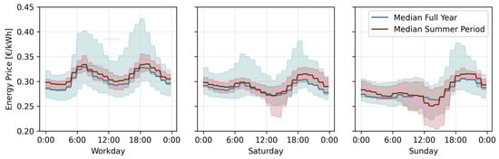
Figure 7. Median energy prices for the full-year period (green) and the summer period (red) in 2021. The 25% and 75% quantiles are in light shaded colors. Energy prices are adjusted by taxes and additional fees to emulate realistic end customer prices. Summer period definition according to H0 SLP [30].

Figure 7. Median energy prices for the full-year period (green) and the summer period (red) in 2021. The 25% and 75% quantiles are in light shaded colors. Energy prices are adjusted by taxes and additional fees to emulate realistic end customer prices. Summer period definition according to H0 SLP [30].

2.7. Optimization Module

To determine the charging schedules, a mixed-integer linear optimization formulation is introduced, extending the approach of Bonin et al. [33] to include DC charging and a terminal SoC constraint. Equation (3) defines the cost function J, which consists of an AC charging component $J_{E,n}^{AC}$, a DC charging component $J_{E,n}^{DC}$, and Lagrange terms $J_{i,n}$ with their corresponding Lagrange multipliers ${\lambda }_i$. The charging schedule optimization is performed using the Pyomo optimization framework [16,17] with the SCIP solver [18], achieving reasonable computation times of a few minutes on an Apple M3 Max chipset.

$$\begin{array}{c}\hfill \begin{array}{ccc}\hfill \underset{\mathit{p},\mathit{q}\in {\mathbb{R}}^N}{min}& \sum _{\begin{array}{c}\forall n\in \mathcal{N}\\ \forall i\in \mathcal{I}\end{array}}\left(J_{E,n}^{AC}+J_{E,n}^{DC}+{\lambda }_i{J}_{i,n}\right)\hfill & \\ \hfill \mathrm{subject}\mathrm{to}& {\underline{\mathbf{p}}}^{EV}\le {\mathbf{p}}^{EV}\le {\overline{\mathbf{p}}}^{EV},{\mathbf{p}}^{EV}\in {\mathbb{R}}^N\hfill & \\ \hfill & {\underline{\mathbf{p}}}^G\le {\mathbf{p}}^G\le {\overline{\mathbf{p}}}^G,{\mathbf{p}}^G\in {\mathbb{R}}^N\hfill & \\ \hfill & {\underline{\mathbf{z}}}^{EV}\le {\mathbf{z}}^{EV}\le {\overline{\mathbf{z}}}^{EV},{\mathbf{z}}^{EV}\in {\mathbb{R}}^N\hfill & \\ & \underline{\mathbf{e}}\le \mathbf{e}\le \overline{\mathbf{e}},\mathbf{e}\in {\mathbb{R}}^{N+1}\hfill \end{array}\end{array}$$

(3)

The decision variables p for AC charging power and z for DC charging power are defined in Equation (4) and Equation (5), respectively. These variables are represented as vectors of length N, corresponding to the optimization horizon. Both decision vectors p and z are bounded by physical constraints from the vehicle equipment $p^{EV}$, $z^{EV}$ and grid infrastructure $p^G$. The state variable e represents the energy content in kWh stored in the high-voltage battery and is similarly bounded by the physical constraints of the battery, as shown in Equation (6).

$${\mathbf{p}}^{EV}={\left(p_0,p_1,\dots ,p_{N-1}\right)}^T\in {{\mathbb{R}}_0^{+}}^N$$

(4)

$${\mathbf{z}}^{EV}={\left(z_0,z_1,\dots ,z_{N-1}\right)}^T\in {{\mathbb{R}}_0^{+}}^N$$

(5)

$$\mathbf{e}={\left(e_0,e_1,\dots ,e_N\right)}^T\in {{\mathbb{R}}_0^{+}}^{N+1}$$

(6)

Among the deterministic variables, $ϵ$ represents AC charging costs, $\kappa$ represents DC charging costs, and s denotes the driving distance in kilometers, as shown in Equations (7)–(9). The dimensionality of all state variables and deterministic vectors is $N+1$, accounting for the final state, where no further decisions are needed.

$$ϵ={\left({ϵ}_0,{ϵ}_1,\dots ,{ϵ}_N\right)}^T\in {\mathbb{R}}^{N+1}$$

(7)

$$\kappa ={\left({\kappa }_0,{\kappa }_1,\dots ,{\kappa }_N\right)}^T\in {\mathbb{R}}^{N+1}$$

(8)

$$\mathbf{s}={\left(s_0,s_1,\dots ,s_N\right)}^T\in {{\mathbb{R}}_0^{+}}^{N+1}$$

(9)

Equations (10) and (11) provide a more detailed description of the AC and DC components of the cost functions, where ${\eta }_p$ and ${\eta }_z$ represent the efficiencies for AC and DC charging, respectively. Charging efficiencies are modeled as static values, which is suitable for this analysis since time-varying constraints on maximum AC charging power are not considered. The optimization algorithm inherently avoids scenarios where vehicles would operate below the rated capacity of their onboard chargers, as part-load charging leads to reduced efficiency.

$$J_{E,n}^{AC}={\displaystyle \frac{1}{{\eta }_p}}·p_n·{ϵ}_n·\Delta t$$

(10)

$$J_{E,n}^{DC}={\displaystyle \frac{1}{{\eta }_z}}·z_n·{\kappa }_n·\Delta t$$

(11)

The state variable e is updated using Equation (12), which captures energy changes resulting from AC and DC charging as well as energy consumption due to driving, thereby maintaining the system’s energy balance. The variable $c_n$ represents the vehicle’s energy consumption with respect to the distance traveled during timeslot n.

$$e_{n+1}=e_n+{\eta }_p·p_n·\Delta t+{\eta }_q·q_n·\Delta t-c_n·s_n$$

(12)

For some charging strategies, charging may be incentivized when the high-voltage battery energy content e falls below a lower threshold $e_{min}$. This can be modeled by incorporating the constraint (13), the binary state variable $\delta$, and the Lagrange term $J_1$; see Equations (14) and (15). When the battery’s energy content drops below $e_{min}$, the binary state variable $\delta$ is set to one. By summing the binary state variable over the optimization horizon and tuning the Lagrange multiplier ${\lambda }_1$, AC or DC charging can be enforced.

$${\displaystyle \frac{e_n-e_{min}}{\overline{e}}}\ge -{\delta }_n$$

(13)

$$\mathsf{\delta }={\left({\delta }_0,{\delta }_1,\dots ,{\delta }_N\right)}^T\in \{0,1\}$$

(14)

$$J_1=\sum _{\begin{array}{c}\forall n\in \mathcal{N}\end{array}}{\delta }_n$$

(15)

The second Lagrange term, $J_2$, ensures that, at the end of the optimization horizon N, the energy content of the EV’s high-voltage battery $e_N$ exceeds the target energy content $e^{*}$, as described in (16). This term can be used to enforce a fully charged vehicle at the end of the optimization horizon.

$$J_2=e^{*}-e_N$$

(16)

2.8. Power Flow Simulation Module

The open-source tool pandapower is used for power flow simulations [19]. For all three municipalities, the distribution grids are modeled in pandapower network models. Building units are connected to the distribution grid through nodes, busbars, and power lines. Household load profiles and EV charging schedules are assigned to their respective nodes within the pandapower network for load flow calculations. The simulations are conducted with a 15 min resolution.

3. Results

The simulation framework is used to perform power flow simulations for three municipalities in the Stuttgart suburbs to assess the impact of EV charging on the distribution grid. To preserve the stochastic nature of the study, each analysis includes 500 simulation runs. The results chapter is structured into three main sections:

• Municipality Overview:This section provides an overview of the three municipalities and their associated distribution grids. It highlights the key characteristics of the synthetically generated population to illustrate the differences between the municipalities and to establish a contextual foundation for the subsequent sensitivity and load flow analyses.
• Sensitivity Analysis: This section identifies the key modeling parameters that significantly impact transformer load and busbar voltage through a sensitivity analysis of various scenarios.
• Load Flow Analysis: For each municipality, a load flow calculation is performed using the key modeling parameters identified in the sensitivity analysis. Different EV penetration rates are explored to assess their impact on transformer load and busbar voltage.

3.1. Municipality Overview

Figure 8, Figure 9, Figure 10, Figure 11, Figure 12 and Figure 13 display the geospatial data of each municipality along with their respective building units, with the number of assigned households represented by a green gradient, as well as the corresponding distribution grid topologies. Open switches indicate disconnected lines within the distribution grid while small red arrows with numbers represent the amount of building units connected to the distribution grid node. To provide a better context for the variability of key parameters across the 500 simulation runs, Table 6, Table 7, Table 8, Table 9, Table 10 and Table 11 are introduced. These tables display the first quartile, median, and third quartile of parameter realizations for each municipality. Table 7, Table 9 and Table 11 provide the relative proportions of each household type, along with their relative differences compared to the MOP dataset across all simulation runs.

• Key Findings:

• Synthetic populations were successfully created for all three municipalities.
• The assignment of mobility profiles based on sociodemographic household attributes aims to identify relevant differences in the simulation results. In two of the three municipalities, the household type distribution deviates by more than 10% from the MOP dataset. Consequently, if these differences have a significant impact, they should be reflected in the simulation results.
• The distribution grids are quite diverse and show varying degrees of meshing. These structural differences are expected to result in observable variations in the minimum busbar voltages.

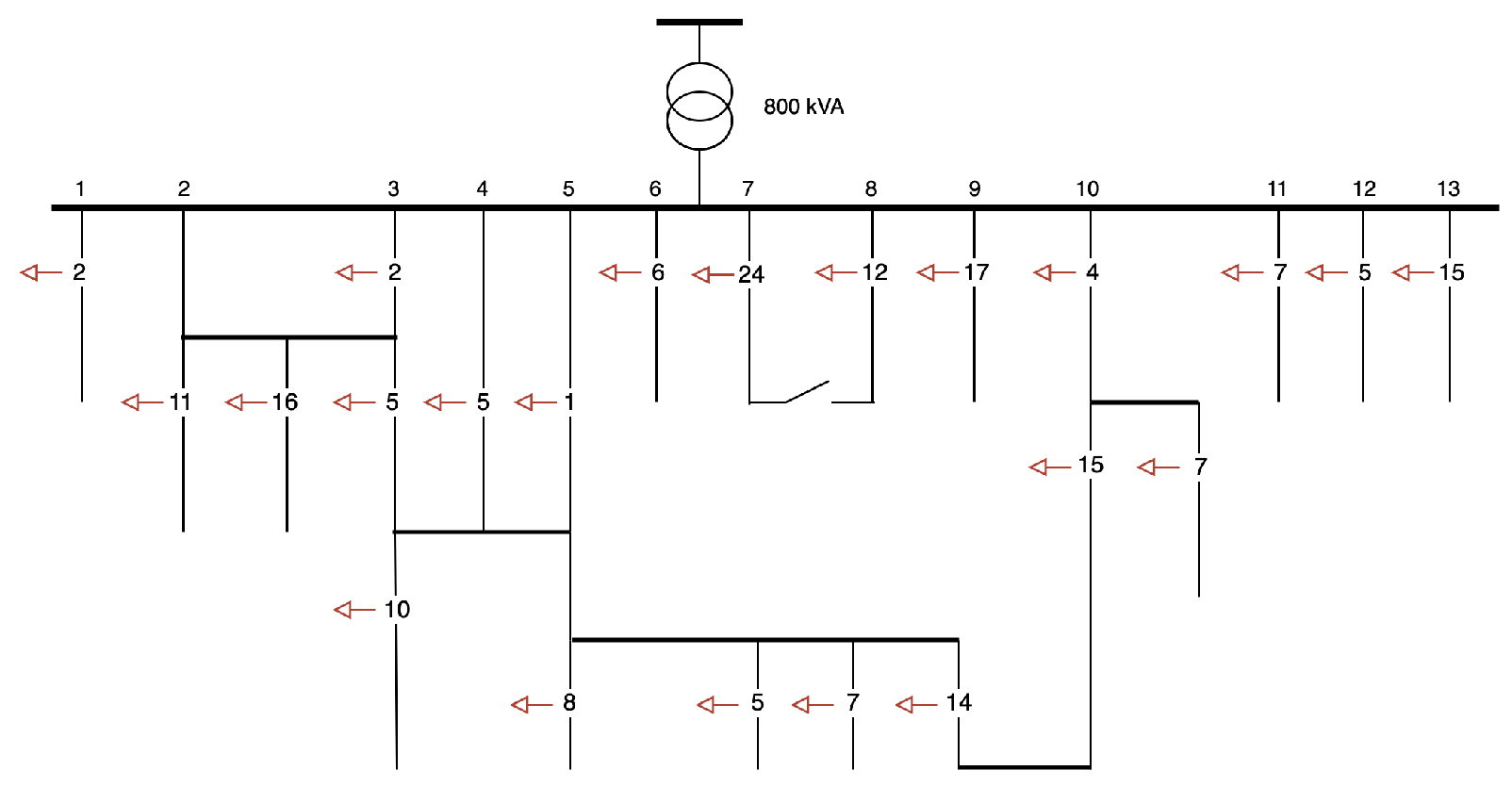
3.1.1. Municipality 1

Municipality 1 is characterized by a cluster of multi-family homes in the southwestern part of the area. The distribution grid topology consists of 11 feeders, an 800 kVA transformer, and 253 connected building units. A decisive feature of Municipality 1 is its demographic composition, with 15.2% fewer type 2 households compared to the statistical average in the MOP dataset. This indicates a notably lower proportion of non-employed or retired persons.

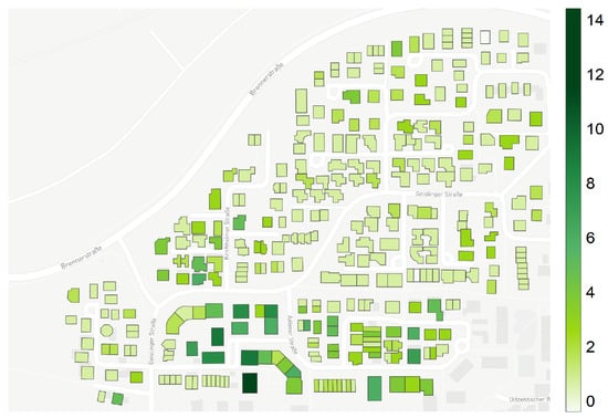
Figure 8. Municipality 1: visualization of the building units with assigned synthetic population. The number of households is represented by a green gradient, with darker areas indicating clusters of multi-family homes.

Figure 8. Municipality 1: visualization of the building units with assigned synthetic population. The number of households is represented by a green gradient, with darker areas indicating clusters of multi-family homes.

Figure 9. Municipality 1: distribution grid topology, featuring an 800 kVA transformer, 11 feeders, and 253 connected buildings. The red arrows with numbers represent the number of connected building units.

Figure 9. Municipality 1: distribution grid topology, featuring an 800 kVA transformer, 11 feeders, and 253 connected buildings. The red arrows with numbers represent the number of connected building units.

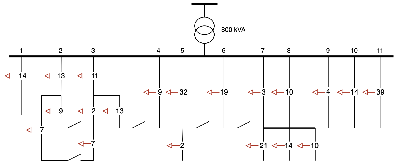
Table 6. Municipality 1: variability of households, persons, and vehicles across 500 simulation runs, showing the 1st quartile (25%), median, and 3rd quartile (75%).

Attribute	1st Quartile (Q1)	Median (Q2)	3rd Quartile (Q3)
Households	466	469	472
Persons	1036	1043	1051
Vehicles	512	553	605

Table 6. Municipality 1: variability of households, persons, and vehicles across 500 simulation runs, showing the 1st quartile (25%), median, and 3rd quartile (75%).

Attribute	1st Quartile (Q1)	Median (Q2)	3rd Quartile (Q3)
Households	466	469	472
Persons	1036	1043	1051
Vehicles	512	553	605

Table 7. Municipality 1: relative distribution of household types across 500 simulation runs and the relative difference to the MOP household type statistics.

Attribute	Community Share [%]	MOP Share [%]	Relative Difference [%]
Household Type 1	45.7	43.1	+2.6
Household Type 2	22.1	37.3	−15.2
Household Type 3	19.1	15.3	+3.8
Household Type 4	13.1	4.3	+8.8

Table 7. Municipality 1: relative distribution of household types across 500 simulation runs and the relative difference to the MOP household type statistics.

Attribute	Community Share [%]	MOP Share [%]	Relative Difference [%]
Household Type 1	45.7	43.1	+2.6
Household Type 2	22.1	37.3	−15.2
Household Type 3	19.1	15.3	+3.8
Household Type 4	13.1	4.3	+8.8

3.1.2. Municipality 2

Municipality 2 is characterized by a cluster of multi-family homes located in the northeastern part of the area, with fewer households and individuals compared to Municipality 1. The distribution grid topology comprises 13 feeders, a 1200 kVA transformer, and 274 connected building units. A defining aspect of Municipality 2 is its demographic profile, with 14.3% fewer type 1 households compared to the statistical average in the MOP dataset. This reflects a significantly lower proportion of 1–2-person-employed households and a higher prevalence of families with three or more persons. The proportion of non-employed retired individuals deviates just slightly from the average in the MOP dataset.

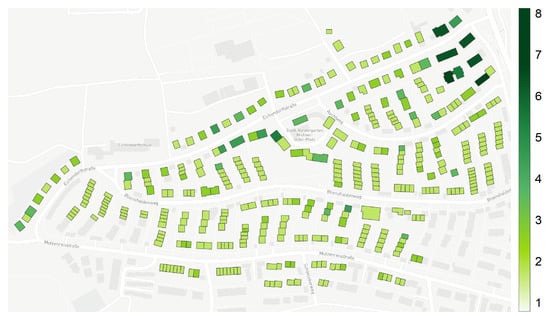
Figure 10. Municipality 2: visualization of the building units with assigned synthetic population. The number of households is represented by a green gradient, with darker areas indicating clusters of multi-family homes.

Figure 10. Municipality 2: visualization of the building units with assigned synthetic population. The number of households is represented by a green gradient, with darker areas indicating clusters of multi-family homes.

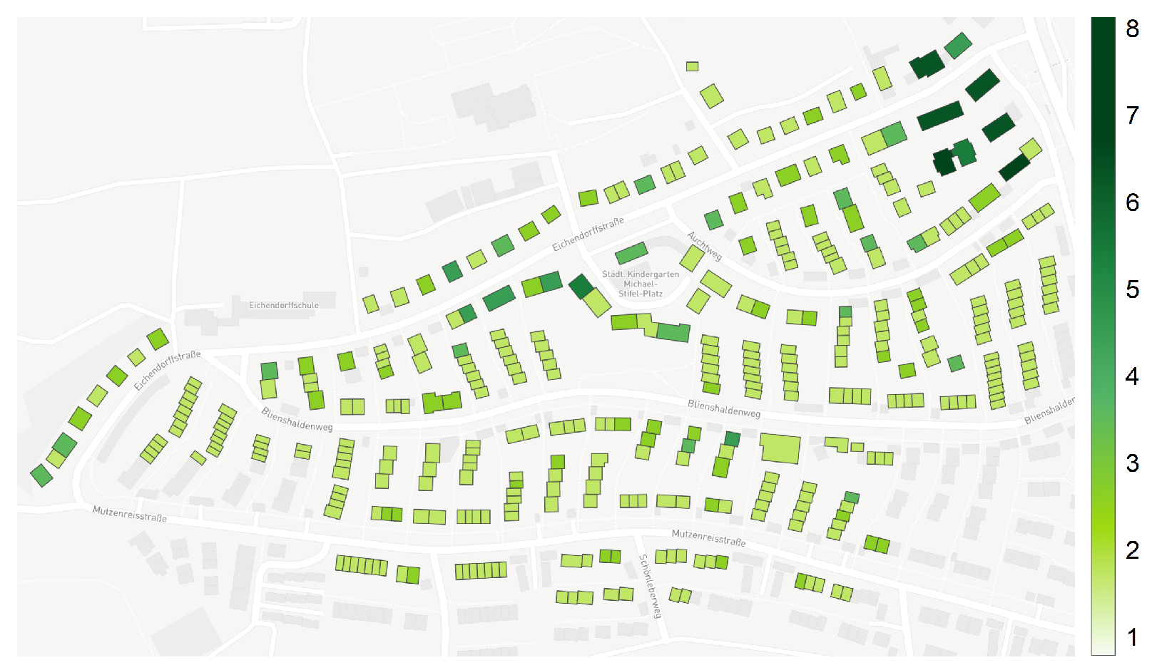
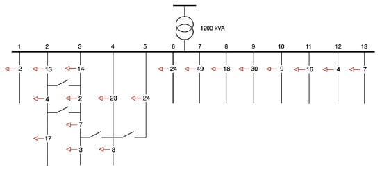
Figure 11. Municipality 2: distribution grid topology, featuring a 1200 kVA transformer, 13 feeders, and 274 connected buildings. The red arrows with numbers represent the number of connected building units.

Figure 11. Municipality 2: distribution grid topology, featuring a 1200 kVA transformer, 13 feeders, and 274 connected buildings. The red arrows with numbers represent the number of connected building units.

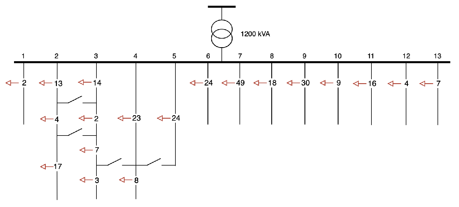
Table 8. Municipality 2: variability of households, persons, and vehicles across 500 simulation runs, showing the 1st quartile (25%), median, and 3rd quartile (75%).

Attribute	1st Quartile (Q1)	Median (Q2)	3rd Quartile (Q3)
Households	362	364	366
Persons	816	823	830
Vehicles	387	419	468

Table 8. Municipality 2: variability of households, persons, and vehicles across 500 simulation runs, showing the 1st quartile (25%), median, and 3rd quartile (75%).

Attribute	1st Quartile (Q1)	Median (Q2)	3rd Quartile (Q3)
Households	362	364	366
Persons	816	823	830
Vehicles	387	419	468

Table 9. Municipality 2: relative distribution of household types across 500 simulation runs and the relative difference to the MOP household type statistics.

Attribute	Community Share [%]	MOP Share [%]	Relative Difference [%]
Household Type 1	28.8	43.1	−14.3
Household Type 2	38.3	37.3	+1.0
Household Type 3	21.4	15.3	+6.1
Household Type 4	11.5	4.3	+7.2

Table 9. Municipality 2: relative distribution of household types across 500 simulation runs and the relative difference to the MOP household type statistics.

Attribute	Community Share [%]	MOP Share [%]	Relative Difference [%]
Household Type 1	28.8	43.1	−14.3
Household Type 2	38.3	37.3	+1.0
Household Type 3	21.4	15.3	+6.1
Household Type 4	11.5	4.3	+7.2

3.1.3. Municipality 3

Municipality 3 is defined by a cluster of multi-family homes located in the central part of the area, with fewer households and individuals compared to Municipality 1. Its distribution grid topology includes 13 feeders, an 800 kVA transformer, and 198 connected building units. An important demographic feature of Municipality 3 is a slightly lower proportion of 1–2-person households and a somewhat higher share of families with three or more persons compared to the statistical average in the MOP dataset, although the differences are less pronounced than in Municipality 2. Additionally, the distribution grid of Municipality 3 has a more meshed configuration compared to those in Municipalities 1 and 2.

Table 10. Municipality 3: variability of households, persons, and vehicles across 500 simulation runs, showing the 1st quartile (25%), median, and 3rd quartile (75%).

Attribute	1st Quartile (Q1)	Median (Q2)	3rd Quartile (Q3)
Households	379	382	385
Persons	807	816	825
Vehicles	401	439	470

Table 10. Municipality 3: variability of households, persons, and vehicles across 500 simulation runs, showing the 1st quartile (25%), median, and 3rd quartile (75%).

Attribute	1st Quartile (Q1)	Median (Q2)	3rd Quartile (Q3)
Households	379	382	385
Persons	807	816	825
Vehicles	401	439	470

Table 11. Municipality 3: relative distribution of household types across 500 simulation runs and the relative difference to the MOP household type statistics.

Attribute	Community Share [%]	MOP Share [%]	Relative Difference [%]
Household Type 1	37.2	43.1	−5.9
Household Type 2	33.6	37.3	−3.7
Household Type 3	19.7	15.3	+4.4
Household Type 4	9.5	4.3	+5.2

Table 11. Municipality 3: relative distribution of household types across 500 simulation runs and the relative difference to the MOP household type statistics.

Attribute	Community Share [%]	MOP Share [%]	Relative Difference [%]
Household Type 1	37.2	43.1	−5.9
Household Type 2	33.6	37.3	−3.7
Household Type 3	19.7	15.3	+4.4
Household Type 4	9.5	4.3	+5.2

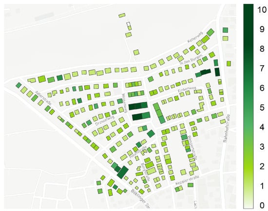
Figure 12. Municipality 3: visualization of the building units with assigned synthetic population. The number of households is represented by a green gradient, with darker areas indicating clusters of multi-family homes.

Figure 12. Municipality 3: visualization of the building units with assigned synthetic population. The number of households is represented by a green gradient, with darker areas indicating clusters of multi-family homes.

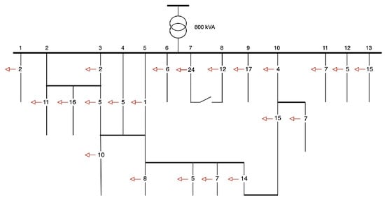
Figure 13. Municipality 3: distribution grid topology, featuring an 800 kVA transformer, 13 feeders, and 198 connected buildings. The red arrows with numbers represent the number of connected building units.

Figure 13. Municipality 3: distribution grid topology, featuring an 800 kVA transformer, 13 feeders, and 198 connected buildings. The red arrows with numbers represent the number of connected building units.

3.2. Sensitivity Analysis

Seven scenarios are analyzed in the sensitivity study, each assuming a fixed presence of 300 EVs. Table 12 provides an overview of the scenario variations. Each scenario is compared to a reference scenario, where EVs are connected to the wallbox after their last trip of the day and remain plugged in until their next trip. Charging occurs at the maximum possible rate without cost optimization. The household baseload and vehicle energy consumption are modeled for calendar week 34 of 2021, representing mild weather conditions. For the cold weather scenario, calendar week 4 of 2021 is modeled. The average vehicle energy consumption is based on the values in Table 5. Figure 14, Figure 15 and Figure 16 illustrate the simulation results across three municipalities. In each figure, the upper graph depicts the transformer peak load, while the lower graph shows the minimum busbar voltage within the distribution grid. Sensitivity results are visualized using boxplots with an interquartile range (IQR) of 1.5. The following subsections describe the scenario variations and results in detail.

Key Findings: The modeling features that consistently exhibit a significant impact on peak transformer load and busbar voltage across all three municipalities are as follows:

• Charging strategy: Whether EVs are charged daily or exclusively on weekends.
• Seasonal effects: Primarily winter, with increased baseload and elevated EV demand.
• AC charging power: Maximum AC charging power of the vehicle’s AC onboard charger (e.g., 11 kW vs. 22 kW).

Modeling features that exhibit a comparable small impact on the results across all municipalities include the following:

• Mobility profile modeling: Assignment based on household size and type, incorporating sociodemographic attributes.
• Biased EV assignment. Higher EV adoption likelihood for single-family and multi-vehicle households.
• Vehicle model: Detailed vehicle class modeling with a diversified and representative vehicle fleet.

Table 12. Sensitivity analysis scenario description.

Parameter	Default	Variation
Model Complexity	Mobility profile assignment based on household size and household type. Unbiased EV assignment	Mobility profile assignment based on household size. Unbiased EV assignment (A1) Mobility profile assignment based on household size and household type. Biased EV assignment (A2)
Charging Strategy	EV charging only at home after the last trip of each day	EV charging only at home after last trip from Friday to Sunday (B1) EV charging at work and at home after each day’s last trip (B2)
Vehicle Model	Diverse and representative vehicle fleet	Average vehicle, charging power 11 kW AC (C1). Average vehicle, charging power 22 kW AC (C2)
Ambient Conditions	Mild Weather CW 34 2021	Cold weather CW 4 2021 (D1)

Table 12. Sensitivity analysis scenario description.

Parameter	Default	Variation
Model Complexity	Mobility profile assignment based on household size and household type. Unbiased EV assignment	Mobility profile assignment based on household size. Unbiased EV assignment (A1) Mobility profile assignment based on household size and household type. Biased EV assignment (A2)
Charging Strategy	EV charging only at home after the last trip of each day	EV charging only at home after last trip from Friday to Sunday (B1) EV charging at work and at home after each day’s last trip (B2)
Vehicle Model	Diverse and representative vehicle fleet	Average vehicle, charging power 11 kW AC (C1). Average vehicle, charging power 22 kW AC (C2)
Ambient Conditions	Mild Weather CW 34 2021	Cold weather CW 4 2021 (D1)

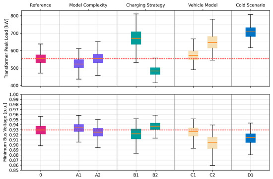
Figure 14. Municipality 1: sensitivity analysis results are presented for seven scenarios, each assuming a fixed count of 300 electric vehicles. Each scenario is depicted using a unique color. The red dotted line indicates the reference scenario, providing visual orientation. Top figure: transformer peak load. Bottom figure: minimum bus voltage within the distribution grid.

Figure 14. Municipality 1: sensitivity analysis results are presented for seven scenarios, each assuming a fixed count of 300 electric vehicles. Each scenario is depicted using a unique color. The red dotted line indicates the reference scenario, providing visual orientation. Top figure: transformer peak load. Bottom figure: minimum bus voltage within the distribution grid.

Figure 15. Municipality 2: sensitivity analysis results are presented for seven scenarios, each assuming a fixed count of 300 electric vehicles. Each scenario is depicted using a unique color. The red dotted line indicates the reference scenario, providing visual orientation. Top figure: transformer peak load. Bottom figure: minimum bus voltage within the distribution grid.

Figure 15. Municipality 2: sensitivity analysis results are presented for seven scenarios, each assuming a fixed count of 300 electric vehicles. Each scenario is depicted using a unique color. The red dotted line indicates the reference scenario, providing visual orientation. Top figure: transformer peak load. Bottom figure: minimum bus voltage within the distribution grid.

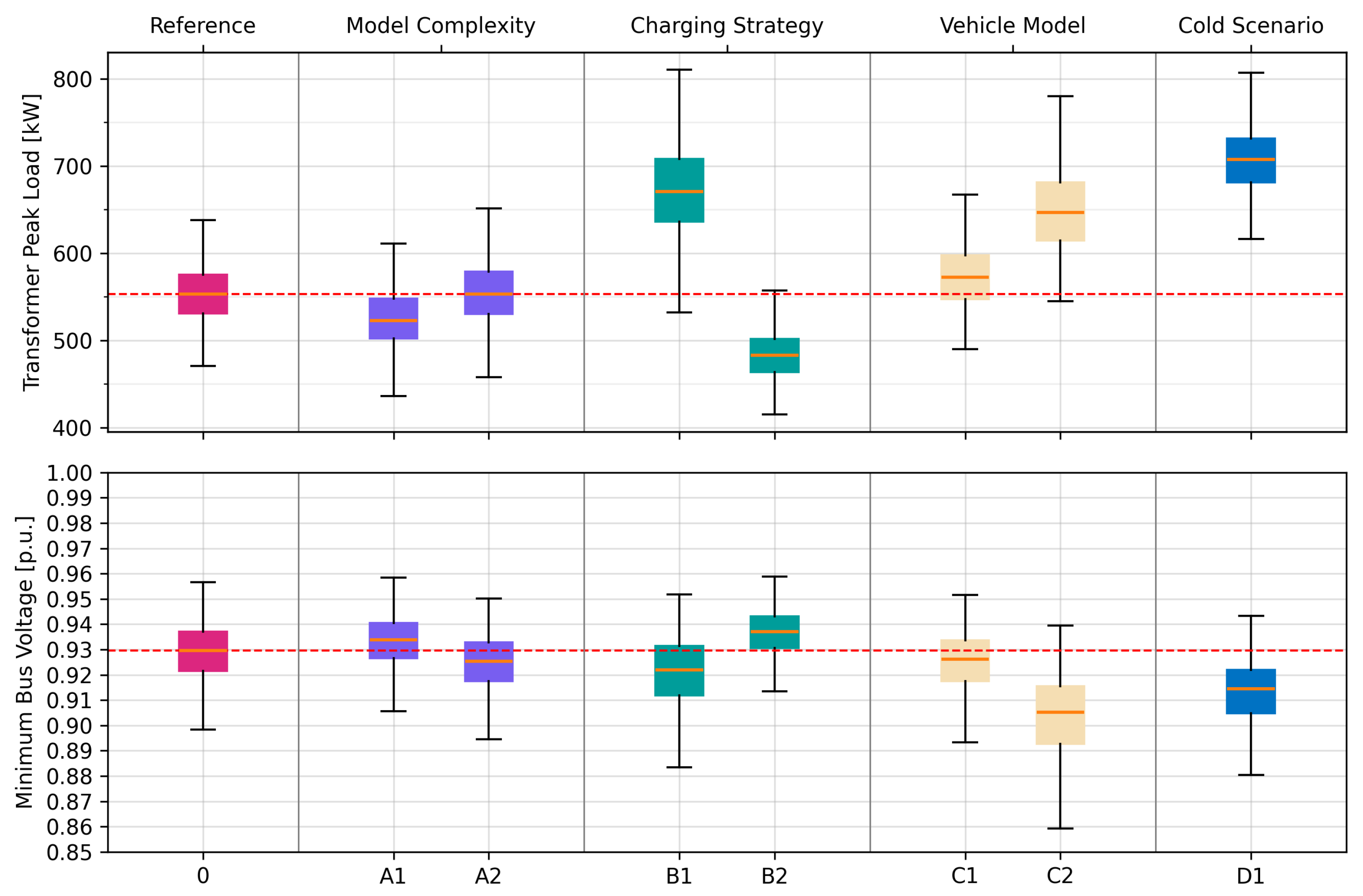
Figure 16. Municipality 3: sensitivity analysis results are presented for seven scenarios, each assuming a fixed count of 300 electric vehicles. Each scenario is depicted using a unique color. The red dotted line indicates the reference scenario, providing visual orientation. Top figure: transformer peak load. Bottom figure: minimum bus voltage within the distribution grid.

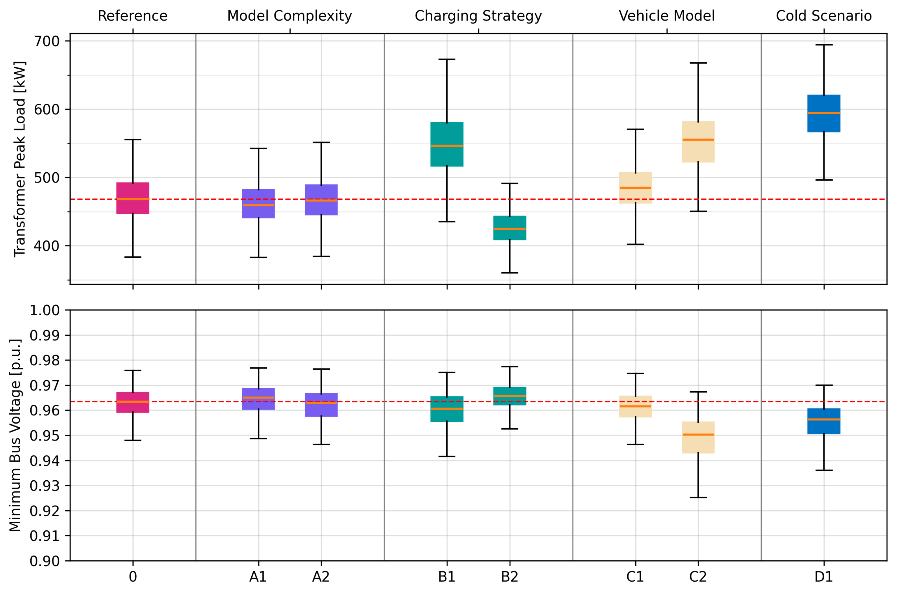
Figure 16. Municipality 3: sensitivity analysis results are presented for seven scenarios, each assuming a fixed count of 300 electric vehicles. Each scenario is depicted using a unique color. The red dotted line indicates the reference scenario, providing visual orientation. Top figure: transformer peak load. Bottom figure: minimum bus voltage within the distribution grid.

3.2.1. Scenario Variation: Model Complexity

• Scenario A1: Mobility profiles are assigned based solely on household size, without considering household type. All other model assumptions remain consistent with the reference scenario. Table 13 presents the median deviation of scenario A1 from the reference scenario for the three municipalities. The comparison shows that Municipality 1 exhibits the largest deviation in transformer peak load, with a 5.5% reduction compared to the reference scenario. In contrast, the deviations in Municipalities 2 and 3 remain below 3%. The pronounced deviation in Municipality 1 is primarily attributed to a significantly lower proportion of household type 2 (retired households), which is 15% lower than the average in the MOP dataset (see Table 7). However, despite this substantial deviation in population characteristics, the overall simulation results remain largely unaffected. Similarly, busbar voltage deviations are minimal and closely align with those of the reference scenario.
• Scenario A2: Mobility profiles are assigned based on household size and type, but EV ownership is biased toward single-family homes with multiple vehicles, which have a higher likelihood of receiving an EV compared to multi-family homes with only one vehicle per household. All other model assumptions remain consistent with the reference scenario. Table 14 presents the median deviation of scenario A2 from the reference scenario for the three municipalities. An analysis shows that biased EV assignment only impacts the median busbar voltage of Municipality 1. For all other municipalities, there is no measurable effect on transformer peak load or minimum busbar voltage.

Table 13. Median deviation of the A1 scenario from the reference scenario for the three municipalities, measured in terms of transformer peak load and minimum bus voltage.

Median Deviation to Reference Scenario	Municipality 1	Municipality 2	Municipality 3
Transformer Peak Load	−5.5%	−1.9%	−2.7%
Minimum Bus Voltage	+0.004 p.u.	+0.002 p.u.	+0.001 p.u.

Table 13. Median deviation of the A1 scenario from the reference scenario for the three municipalities, measured in terms of transformer peak load and minimum bus voltage.

Median Deviation to Reference Scenario	Municipality 1	Municipality 2	Municipality 3
Transformer Peak Load	−5.5%	−1.9%	−2.7%
Minimum Bus Voltage	+0.004 p.u.	+0.002 p.u.	+0.001 p.u.

Table 14. Median deviation of scenario A1 from the reference scenario for the three municipalities, measured in terms of transformer peak load and minimum bus voltage.

Median Deviation to Reference Scenario	Municipality 1	Municipality 2	Municipality 3
Transformer Peak Load	+0.0%	+0.0%	+0.0%
Minimum Bus Voltage	−0.004 p.u.	−0.000 p.u.	−0.000 p.u.

Table 14. Median deviation of scenario A1 from the reference scenario for the three municipalities, measured in terms of transformer peak load and minimum bus voltage.

Median Deviation to Reference Scenario	Municipality 1	Municipality 2	Municipality 3
Transformer Peak Load	+0.0%	+0.0%	+0.0%
Minimum Bus Voltage	−0.004 p.u.	−0.000 p.u.	−0.000 p.u.

3.2.2. Scenario Variation: Charging Strategy

• Scenario B1: EV charging only at home after the last trip from Friday to Sunday. All other model assumptions remain consistent with the reference scenario. Table 15 presents the median deviation of scenario B1 from the reference scenario across the three municipalities. For all three municipalities, a notable increase in transformer peak load of up to 25% is observed. Additionally, minimum busbar voltages decrease noticeably, and the variance increases. The delayed charging until Friday results in higher energy demand, which not only extends charging times but also increases the likelihood of simultaneous EV charging.
• Scenario B2: EV charging at work and at home after each day’s last trip. Unlike the previous scenarios, the vehicle is now also charged at the workplace. All other model assumptions remain consistent with the reference scenario. Table 16 presents the median deviation of scenario B2 from the reference scenario across the three municipalities. For all three municipalities, a notable decrease in the transformer peak load of more than 12% is observed. Charging at the workplace reduces the amount of charging at home, which mitigates the occurrence of simultaneous charging events. This is reflected in a lower transformer peak load, as well as a more relaxed minimum busbar voltage with reduced variance.

Table 15. Median deviation of scenario B1 from the reference scenario for the three municipalities, measured in terms of transformer peak load and minimum bus voltage.

Median Deviation to Reference Scenario	Municipality 1	Municipality 2	Municipality 3
Transformer Peak Load	+21.2%	+16.7%	+25.1%
Minimum Bus Voltage	−0.008 p.u.	−0.003 p.u.	−0.007 p.u.

Table 15. Median deviation of scenario B1 from the reference scenario for the three municipalities, measured in terms of transformer peak load and minimum bus voltage.

Median Deviation to Reference Scenario	Municipality 1	Municipality 2	Municipality 3
Transformer Peak Load	+21.2%	+16.7%	+25.1%
Minimum Bus Voltage	−0.008 p.u.	−0.003 p.u.	−0.007 p.u.

Table 16. Median deviation of scenario B2 from the reference scenario for the three municipalities, measured in terms of transformer peak load and minimum bus voltage.

Median Deviation to Reference Scenario	Municipality 1	Municipality 2	Municipality 3
Transformer Peak Load	−12.7%	−9.3%	−12.2%
Minimum Bus Voltage	+0.008 p.u.	+0.002 p.u.	+0.004 p.u.

Table 16. Median deviation of scenario B2 from the reference scenario for the three municipalities, measured in terms of transformer peak load and minimum bus voltage.

Median Deviation to Reference Scenario	Municipality 1	Municipality 2	Municipality 3
Transformer Peak Load	−12.7%	−9.3%	−12.2%
Minimum Bus Voltage	+0.008 p.u.	+0.002 p.u.	+0.004 p.u.

3.2.3. Scenario Variation: Vehicle Model

• Scenario C1: Average vehicle with maximum AC charging power of 11 kW. In this scenario, the statistical vehicle type modeling is replaced by the average vehicle parameters from Table 5. The average AC charging power of 10.4 kW is replaced with 11 kW, which is the next feasible value for standard onboard chargers available in EVs. All other model assumptions remain consistent with the reference scenario.
  A comparison of the median deviations in Table 17 reveals that the relative deviation in transformer peak load remains below 4%, while the deviation in minimum busbar voltage is nearly negligible. These results suggest that replacing a detailed vehicle type model with a simplified average vehicle model is a valid approach, as other modeling factors effectively outweigh potential inaccuracies introduced by using an average vehicle model.
• Scenario C2: Average vehicle with maximum AC charging power of 22 kW.
  In this scenario, the statistical vehicle type modeling is replaced with the average vehicle parameters from Table 5, assuming an AC charging power of 22 kW for every EV. All other model assumptions remain consistent with the reference scenario.
  As expected, the increase in charging power leads to a significant rise in median transformer peak loads, ranging from 15% to 18%, as shown in Table 18. This also has a considerable impact on the minimum busbar voltages in the distribution grid. Although the charging power is twice as high as in the base scenario, the peak loads for EVs are not doubled. This can be explained by the fact that faster charging reduces the overall charging duration, thereby decreasing the number of simultaneous charging events. A large-scale shift from 11 kW to 22 kW charging power in future EVs would certainly have considerable impacts. However, most current EVs are equipped with 11 kW onboard chargers, and a widespread shift to 22 kW chargers is not yet foreseeable.

Table 17. Median deviation of scenario C1 from the reference scenario for the three municipalities, measured in terms of transformer peak load and minimum bus voltage.

Median Deviation to Reference Scenario	Municipality 1	Municipality 2	Municipality 3
Transformer Peak Load	+3.4%	+3.7%	+0.2%
Minimum Bus Voltage	−0.003 p.u.	−0.002 p.u.	−0.000 p.u.

Table 17. Median deviation of scenario C1 from the reference scenario for the three municipalities, measured in terms of transformer peak load and minimum bus voltage.

Median Deviation to Reference Scenario	Municipality 1	Municipality 2	Municipality 3
Transformer Peak Load	+3.4%	+3.7%	+0.2%
Minimum Bus Voltage	−0.003 p.u.	−0.002 p.u.	−0.000 p.u.

Table 18. Median deviation of scenario C2 from the reference scenario for the three municipalities, measured in terms of transformer peak load and minimum bus voltage.

Median Deviation to Reference Scenario	Municipality 1	Municipality 2	Municipality 3
Transformer Peak Load	+16.9%	+18.6%	+15.0%
Minimum Bus Voltage	−0.024 p.u.	−0.013 p.u.	−0.009 p.u.

Table 18. Median deviation of scenario C2 from the reference scenario for the three municipalities, measured in terms of transformer peak load and minimum bus voltage.

Median Deviation to Reference Scenario	Municipality 1	Municipality 2	Municipality 3
Transformer Peak Load	+16.9%	+18.6%	+15.0%
Minimum Bus Voltage	−0.024 p.u.	−0.013 p.u.	−0.009 p.u.

3.2.4. Scenario Variation: Ambient Conditions

• Scenario D1: Scenario D1 models cold weather conditions. Two key factors distinguish this scenario from all others. First, the vehicle consumption is higher, following the values in Table 5. Second, the household load is elevated, due to the winter period. All other model assumptions remain consistent with the reference scenario.
  Table 19 illustrates that the transformer peak load is approximately 27% higher than in the reference scenario. This effect is also reflected in a more pronounced minimum busbar voltage. These results highlight the critical impact of EV charging during winter periods. In conclusion, cold weather conditions have a huge impact on the power flow simulation results across all three municipalities, far outweighing other modeling factors, such as biased EV assignment or mobility modeling based on sociodemographic attributes.

Table 19. Median deviation of scenario D1 from the reference scenario for the three municipalities, measured in terms of transformer peak load and minimum bus voltage.

Median Deviation to Reference Scenario	Municipality 1	Municipality 2	Municipality 3
Transformer Peak Load	+27.9%	+27.0%	+27.0%
Minimum Bus Voltage	−0.015 p.u.	−0.007 p.u.	−0.010 p.u.

Table 19. Median deviation of scenario D1 from the reference scenario for the three municipalities, measured in terms of transformer peak load and minimum bus voltage.

Median Deviation to Reference Scenario	Municipality 1	Municipality 2	Municipality 3
Transformer Peak Load	+27.9%	+27.0%	+27.0%
Minimum Bus Voltage	−0.015 p.u.	−0.007 p.u.	−0.010 p.u.

3.3. Power Flow Simulation Results

Finally, load flow calculations are performed for the three municipalities at varying EV penetration rates. The analyzed scenarios include the ‘Reference Scenario’, the ‘Weekend Charging Scenario,’ and a cost-optimized charging scenario that models EV charging based on day-ahead EEX price data from 2021, as described in the ‘Charging Price Module’ chapter. To ensure a worst-case assessment, the cold weather scenario is applied to all cases.

• Key Findings:

• Cost-optimized charging has the greatest impact on the distribution grids. In two of the three municipalities, transformer overloads occur even at relatively moderate local EV penetration rates of 20 to 25%.
• In all other scenarios, no transformer overloads are expected up to relatively high penetration rates of 75%.
• Minimum busbar voltage violations consistently occur earlier than transformer overloads.
• The degree of meshing in the distribution grids plays a significant role. A clear trend is observed across Municipalities 1 to 3, with increasing meshing corresponding to a decreasing proportion of feeders affected by voltage violations. This underlines the critical importance of detailed distribution grid modeling for accurate impact assessment.

Figure 17, Figure 18 and Figure 19 present the results for the three communities, with each figure consisting of two graphs. The upper graph illustrates the transformer peak load as a function of the number of EVs. Distinct colors represent the different scenarios. The red horizontal line indicates the maximum transformer capacity, serving as a reference for identifying transformer overload conditions. The lower diagram presents the relative proportion of feeders experiencing voltage band violations, defined as instances where the minimum busbar voltage falls below 0.95 p.u. To provide a clearer understanding of the severity of these violations, the median is represented by a dashed line while the 99th percentile is shown as a solid line. A distinct feature of Municipality 2 is its significantly higher maximum transformer capacity of 1200 kVA compared to Municipalities 1 and 3.

A comparison of the figures indicates that, even under the cold weather scenario, the transformer can accommodate up to 250 EVs in all non-cost-optimized charging scenarios. Cross-referencing these results with the average number of vehicles per municipality, as detailed in Table 6, Table 8, and Table 10, results in local EV penetration rates of 45% to 59%. However, it is important to note that the transformer capacity is not the limiting factor. Instead, voltage band violations on the feeders represent the critical constraint. Assuming that 20% of feeders could be reinforced with an adequate lead time, the achievable EV penetration strongly varies with the characteristics of the distribution grid. For example, in Municipality 1, feeder constraints are violated with just 100 EVs, equating to an 18% penetration rate, while in Municipality 3, with its higher meshing, up to 200 EVs, or a 45% penetration rate, could be accommodated. This wide range underlines the need for detailed modeling of grid topology to assess the local capacity for EV integration. Regarding cost-optimized charging strategies, it is important to note that even a relatively small number of 50 electric vehicles can cause significant bottlenecks. With 100 electric vehicles, the maximum transformer capacity exceeds the median in nearly all cases.

Figure 20 further illustrates the impact of a purely cost-optimized charging strategy on Community 1 during the winter months. It presents the 75th percentile of transformer peak load and the average charging cost over one week for 100 EVs and the three scenarios. The results clearly show that cost-optimized charging can cause significant transformer load peaks. Even when charging occurs during baseload valleys, the maximum transformer load can still double. These findings underscore the importance of integrating cost-optimized charging with intelligent control mechanisms to manage the maximum available charging power. Such measures should be implemented even at low local EV penetration rates, as market-driven incentives can lead to synchronized charging behavior. Additionally, many users are more likely to charge their vehicles on weekends for convenience, leading to longer charging sessions and a higher chance of simultaneous charging events. When combined with cost-optimization strategies, this clustering effect can significantly increase grid stress and potentially cause critical overload conditions. Challenges already arise in the early stages of the EV ramp-up scenario, where the simultaneity of charging events does not have a counteracting effect on energy prices, such as price increases.

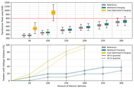
Figure 17. Municipality 1: power flow simulation results for different charging strategies. Top figure: transformer peak load as a function of the number of EVs, with the red horizontal line representing the maximum transformer capacity. Bottom figure: relative share of feeders experiencing voltage band violations, defined as instances where the minimum feeder voltage drops below 0.95 p.u. The median is shown as a dashed line, and the 99th percentile is depicted as a solid line.

Figure 17. Municipality 1: power flow simulation results for different charging strategies. Top figure: transformer peak load as a function of the number of EVs, with the red horizontal line representing the maximum transformer capacity. Bottom figure: relative share of feeders experiencing voltage band violations, defined as instances where the minimum feeder voltage drops below 0.95 p.u. The median is shown as a dashed line, and the 99th percentile is depicted as a solid line.

Figure 18. Municipality 2: power flow simulation results for different charging strategies. Top figure: transformer peak load as a function of the number of EVs, with the red horizontal line representing the maximum transformer capacity. Bottom figure: relative share of feeders experiencing voltage band violations, defined as instances where the minimum feeder voltage drops below 0.95 p.u. The median is shown as a dashed line, and the 99th percentile is depicted as a solid line.

Figure 18. Municipality 2: power flow simulation results for different charging strategies. Top figure: transformer peak load as a function of the number of EVs, with the red horizontal line representing the maximum transformer capacity. Bottom figure: relative share of feeders experiencing voltage band violations, defined as instances where the minimum feeder voltage drops below 0.95 p.u. The median is shown as a dashed line, and the 99th percentile is depicted as a solid line.

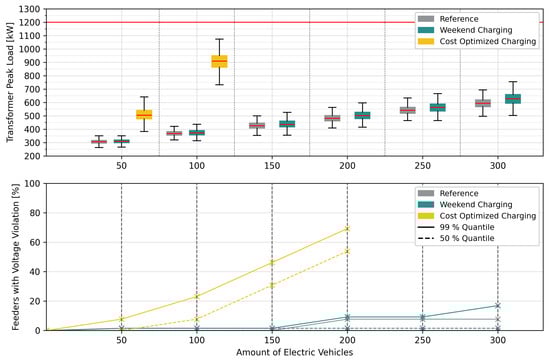
Figure 19. Municipality 3: power flow simulation results for different charging strategies. Top figure: transformer peak load as a function of the number of EVs, with the red horizontal line representing the maximum transformer capacity. Bottom figure: relative share of feeders experiencing voltage band violations, defined as instances where the minimum feeder voltage drops below 0.95 p.u. The median is shown as a dashed line, and the 99th percentile is depicted as a solid line.

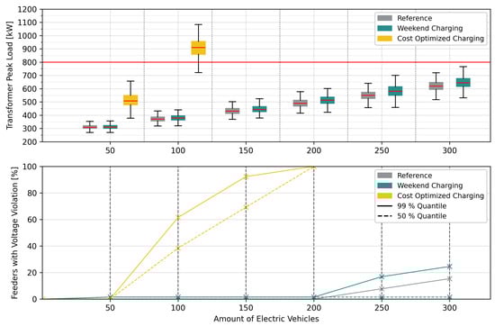
Figure 19. Municipality 3: power flow simulation results for different charging strategies. Top figure: transformer peak load as a function of the number of EVs, with the red horizontal line representing the maximum transformer capacity. Bottom figure: relative share of feeders experiencing voltage band violations, defined as instances where the minimum feeder voltage drops below 0.95 p.u. The median is shown as a dashed line, and the 99th percentile is depicted as a solid line.

Figure 20. Municipality 1: transformer peak load impact by different charging strategies. Top figure: comparison of 75th percentile of transformer peak load for different charging strategies over 1 week for 100 EVs (20% local EV share). The maximum transformer load is represented by the red horizontal line. Bottom figure: mean charging cost during winter months of 2021. Energy prices are based on EEX data, adjusted for taxes and additional fees to reflect realistic end-customer prices [32].

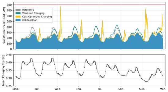
Figure 20. Municipality 1: transformer peak load impact by different charging strategies. Top figure: comparison of 75th percentile of transformer peak load for different charging strategies over 1 week for 100 EVs (20% local EV share). The maximum transformer load is represented by the red horizontal line. Bottom figure: mean charging cost during winter months of 2021. Energy prices are based on EEX data, adjusted for taxes and additional fees to reflect realistic end-customer prices [32].

4. Discussion

This study introduced a modular simulation framework to assess the impact of electric vehicle (EV) charging on the distribution grids of three real-world municipalities. A sensitivity analysis was conducted assuming a high local EV penetration, with 300 EVs out of a total vehicle stock ranging from 387 to 605 per municipality. The analysis focused on evaluating the effects of different scenarios on transformer peak load and minimum busbar voltage. Based on the results of the sensitivity analysis, subsequent power flow simulations with varying EV penetration levels were performed.

4.1. Sensitivity Analysis

The following modeling features were identified as having a significant and consistent impact on transformer peak load and busbar voltage across all three municipalities:

• Charging Strategy: The choice between charging vehicles at home daily or only on weekends has a comparably strong impact. This observation aligns with findings from Fischer et al. [8] and Stiasny et al. [9], although these studies did not provide detailed sociodemographic modeling or analyze effects on busbar voltage. The results of this study indicate that charging EVs solely on weekends can cause a significant clustering of charging events, leading to an increase in the transformer peak load of up to 25%. Extending the analysis to minimum busbar voltage, we find a relatively small median reduction of approximately 0.01 p.u. However, the variance in voltage deviations increases substantially, with individual events deviating by as much as 0.05 p.u. from the reference scenario. This is a crucial finding, as even rare and unlikely events have the potential to compromise distribution grid stability.
  Conversely, charging electric vehicles on a daily basis, both at home and at workplaces, can reduce the transformer peak load by up to 13%. The positive impact on minimum busbar voltage is minimal, with changes below 0.01 p.u. and no noticeable increase in voltage variance compared to the reference scenario. Overall, these findings warrant serious consideration, as charging EVs primarily on weekends is both practically relevant and likely, since daily charging often reduces user convenience.
• Seasonal Effects: An increased baseload and higher EV demand during winter led to a relative transformer peak load increase of up to 28%, along with a median reduction of up to 0.015 p.u. in minimum busbar voltage. The high relevance of seasonal effects is increasingly recognized in the literature, as the growing adoption of EVs is expected to coincide with the widespread deployment of heat pumps, further increasing stress on the distribution grid during winter season [34].
• Maximum AC Charging Power: Consistent with the findings of [9], the maximum AC charging power of EVs was found to be a significant factor for transformer peak load. This study builds on their results by also quantifying the impact on minimum busbar voltage, revealing both a notable decrease in the median voltage and a substantial increase in variance. Across the three municipalities studied, equipping all future vehicles with 22 kW AC onboard chargers could lead to up to a 19% increase in transformer peak load and a reduction in minimum busbar voltage by 0.024 p.u. However, from a practical perspective, a widespread shift from 11 kW to 22 kW AC onboard-chargers in future EVs is unlikely. Consequently, compared to the other two findings, this scenario appears primarily theoretical.

By contrast, the following features showed only a limited impact across all three municipalities:

• Mobility patterns from the MOP dataset were assigned based on sociodemographic attributes such as household size and household type, indirectly reflecting occupation-related factors known to influence mobility behavior [8]. Previous studies have shown that sampling from different mobility datasets can affect simulation outcomes, although the impact is generally smaller than that of other factors, such as charging behavior, local electric vehicle adoption, and the type of charging infrastructure [9]. The present study confirms this observation. Even when applying detailed modeling based on a synthetic population calibrated for the analyzed municipalities, the influence remains smaller than that of other scenario parameters. Variations in median transformer peak load remained below 6 percent, and changes in busbar voltage stayed within 0.01 per unit across all three municipalities. While it is well established that sociodemographic and socioeconomic characteristics influence individual charging behavior, and that differences between user groups can be observed [8], this study explored how such effects aggregate within real municipal populations, which typically consist of a heterogeneous mix of user profiles rather than uniform groups. The results also align with the findings of [35], who reported impacts of up to 8% on median transformer peak load and less than 1% on busbar voltage deviation when mobility patterns were modeled based on sociodemographic characteristics. However, they also noted that the impact becomes more pronounced when mobility modeling is combined with the allocation of charging points according to sociodemographic attributes. Overall, this study extends previous work by demonstrating that, even with detailed synthetic population modeling and mobility pattern assignment based on sociodemographic data, the effects on transformer peak loads and minimum busbar voltages remain relatively minor compared to other sources of uncertainty. This is a reassuring result, as such modeling requires highly detailed and spatially disaggregated input data, which is rarely available.
• Biased EV Assignment: The preferential assignment of electric vehicles to households with a higher likelihood of adoption, such as those living in single-family homes or owning multiple vehicles, has a limited impact. Similar conclusions were drawn by Stiasny et al. [9], who found that even, mildly clustered, and heavily clustered distributions yielded comparable results. The findings presented here build on this, showing that the conclusion remains valid when more detailed modeling of population and sociodemographic mobility is applied, and when the analysis is extended to include effects on busbar voltage. A potential exception may be individual streets or neighborhoods with an unusually high share of electric vehicles. However, such cases should be manageable for distribution grid operators, as charging points are typically registered. Designing distribution networks universally to account for these rare cases would be excessive and unnecessary.
• Detailed Vehicle Class Modeling: Differentiating between specific vehicle classes results in less than a 3% impact on transformer load and has a negligible effect on busbar voltages. Consequently, modeling vehicles using an average consumption profile, as shown in Table 5, is sufficient for distribution grid analysis. While Fischer et al. [8] observed variations when analyzing small, mid-sized, and large vehicles next to each other, real-world vehicle fleets consist of a mix of vehicle types, leading to an averaging effect. This effect, previously demonstrated by Stiasny et al. [9] for transformer peak loads, is now also confirmed for busbar voltage behavior.

Although the attributes identified as less relevant may have greater importance in early market ramp-up scenarios, this study deliberately focused on conditions of high electric vehicle penetration, as these are most critical for assessing the risk of local distribution grid overloading.

4.2. Power Flow Simulation

Following the sensitivity analysis, a power flow simulation was conducted for the same three municipalities, this time focusing on the most critical factors identified in the analysis and considering varying levels of local EV penetration. Three charging scenarios were examined: first, the reference scenario from the sensitivity analysis; second, a weekend charging scenario, based on the assumption that users prefer charging their EVs on weekends for convenience; and third, a cost-optimized charging scenario, in which charging aligns with periods of low electricity prices. All simulations were carried out under winter conditions to reflect seasonal peak loads and increased EV consumption.

The results clearly show that cost-optimized charging places significantly greater stress on the distribution grids than either of the other scenarios, causing transformer overloads in two of the three municipalities at local EV penetration levels as low as 20 to 25%. By contrast, the non-cost-optimized scenarios did not exceed transformer capacity limits even at high penetration rates of around 75%. As dynamic electricity tariffs become widespread, understanding their influence on charging behavior will be essential for ensuring a safe and reliable operation of distribution grids. This conclusion is also supported by several studies, including [33,36,37]. While limiting charging power may appear to be a straightforward mitigation strategy, it is not recommended, as periods of low electricity prices often coincide with high levels of renewable generation. Thus, promoting EV charging during these times directly contributes to decarbonization efforts. Therefore, regulatory and technical measures should focus on enabling the coordinated, grid-friendly implementation of market-based charging strategies. Beyond the impact of cost-optimized charging, the simulation results also reveal that voltage limit violations typically occur well before transformer overloads, highlighting the need to jointly assess voltage stability and transformer loading in grid impact analyses. The findings also demonstrate that grid topology, particularly the degree of meshing, plays a decisive role in determining the EV hosting capacity of distribution networks. These insights underscore the importance of accurately representing grid structures when conducting real-world assessments.

4.3. Outlook

It is recommended that future research focus on two key aspects. First, the cold weather scenario should be expanded to include heat pumps, which are expected to further intensify peak electricity demand during winter season. Second, coordination strategies for cost-optimized EV charging require thorough investigation, as uncoordinated price-based charging could overload distribution grids even at early stages of EV adoption, with local penetration rates below 20%. Ideally, these strategies should incorporate additional optimization objectives, such as maximizing self-consumption from photovoltaic systems and home battery storage, particularly in conjunction with bidirectional AC charging.

References

- Umweltbundesamt. Analyse der Umweltbilanz von Kraftfahrzeugen mit Alternativen Antrieben oder Kraftstoffen auf dem Weg zu Einem Treibhausgasneutralen Verkehr; Umweltbundesamt: Dessau-Roßlau, Germany, 2024. [Google Scholar] [CrossRef]
- Hardman, S.; Jenn, A.; Tal, G.; Axsen, J.; Beard, G.; Daina, N.; Figenbaum, E.; Jakobsson, N.; Jochem, P.; Kinnear, N.; et al. A review of consumer preferences of and interactions with electric vehicle charging infrastructure. Transp.Res. Part D Transp. Environ. 2018, 62, 508–523. [Google Scholar] [CrossRef]
- Dubey, A.; Santoso, S. Electric Vehicle Charging on Residential Distribution Systems: Impacts and Mitigations. IEEE Access 2015, 3, 1871–1893. [Google Scholar] [CrossRef]
- Clement-Nyns, K.; Haesen, E.; Driesen, J. The Impact of Charging Plug-In Hybrid Electric Vehicles on a Residential Distribution Grid. IEEE Trans. Power Syst. 2010, 25, 371–380. [Google Scholar] [CrossRef]
- Galus, M.D.; Waraich, R.A.; Balmer, M.; Andersson, G.; Axhausen, K.W. A Framework for Investigating the Impact of PHEVS; ETH Library: Zurich, Switzerland, 2009. [Google Scholar] [CrossRef]
- Waraich, R.A.; Galus, M.D.; Dobler, C.; Balmer, M.; Andersson, G.; Axhausen, K.W. Plug-in hybrid electric vehicles and smart grids: Investigations based on a microsimulation. Transp. Res. Part C Emerg. Technol. 2013, 28, 74–86. [Google Scholar] [CrossRef]
- Gschwendtner, C.; Knoeri, C.; Stephan, A. The impact of plug-in behavior on the spatial–temporal flexibility of electric vehicle charging load. Sustain. Cities Soc. 2023, 88, 104263. [Google Scholar] [CrossRef]
- Fischer, D.; Harbrecht, A.; Surmann, A.; McKenna, R. Electric vehicles’ impacts on residential electric local profiles—A stochastic modelling approach considering socio-economic, behavioural and spatial factors. Appl. Energy 2019, 233–234, 644–658. [Google Scholar] [CrossRef]
- Stiasny, J.; Zufferey, T.; Pareschi, G.; Toffanin, D.; Hug, G.; Boulouchos, K. Sensitivity analysis of electric vehicle impact on low-voltage distribution grids. Electr. Power Syst. Res. 2021, 191, 106696. [Google Scholar] [CrossRef]
- Karmaker, A.K.; Behrens, S.; Pota, H. Sensitivity Analysis for Electric Vehicle Hosting Capacity in Distribution Networks. In Proceedings of the 2023 IEEE Transportation Electrification Conference and Expo, Asia-Pacific (ITEC Asia-Pacific), Chiang Mai, Thailand, 28 November–1 December 2023; pp. 1–7. [Google Scholar] [CrossRef]
- Fani, H.; Hashmi, M.U.; Deconinck, G. Impact of electric vehicle charging simultaneity factor on the hosting capacity of LV feeder. Sustain. Energy Grids Netw. 2024, 40, 101581. [Google Scholar] [CrossRef]
- Held, L.; Märtz, A.; Krohn, D.; Wirth, J.; Zimmerlin, M.; Suriyah, M.R.; Leibfried, T.; Jochem, P.; Fichtner, W. The Influence of Electric Vehicle Charging on Low Voltage Grids with Characteristics Typical for Germany. World Electr. Veh. J. 2019, 10, 88. [Google Scholar] [CrossRef]
- DIN EN 50160:2020-11; Voltage Characteristics of Electricity Supplied by Public Electricity Networks. DIN Deutsches Institut für Normung e.V., Beuth Verlag: Berlin, Germany, 2010.
- BMVI. German Mobility Panel (MOP): Longitudinal Study on the Travel Behavior of the Population; Federal Ministry of Transport and Digital Infrastructure (BMVI): Berlin, Germany. Available online: https://mobilitaetspanel.ifv.kit.edu/english/index.php (accessed on 18 July 2024).
- Electric Vehicle Database. Current and Upcoming Electric Vehicles. Available online: https://ev-database.org/ (accessed on 25 July 2024).
- Bynum, M.L.; Hackebeil, G.A.; Hart, W.E.; Laird, C.D.; Nicholson, B.L.; Siirola, J.D.; Watson, J.P.; Woodruff, D.L. Pyomo–Optimization Modeling in Python, 3rd ed.; Springer Science & Business Media: Cham, Switzerland, 2021; Volume 67. [Google Scholar]
- Hart, W.E.; Watson, J.P.; Woodruff, D.L. Pyomo: Modeling and solving mathematical programs in Python. Math. Program. Comput. 2011, 3, 219–260. [Google Scholar] [CrossRef]
- Bolusani, S.; Besançon, M.; Bestuzheva, K.; Chmiela, A.; Dionísio, J.; Donkiewicz, T.; van Doornmalen, J.; Eifler, L.; Ghannam, M.; Gleixner, A.; et al. The SCIP Optimization Suite 9.0; Technical Report; Optimization Online: Berlin, Germany, 2024. [Google Scholar]
- Thurner, L.; Scheidler, A.; Schafer, F.; Menke, J.H.; Dollichon, J.; Meier, F.; Meinecke, S.; Braun, M. Pandapower—An Open-Source Python Tool for Convenient Modeling, Analysis, and Optimization of Electric Power Systems. IEEE Trans. Power Syst. 2018, 33, 6510–6521. [Google Scholar] [CrossRef]
- Statistisches Bundesamt. Zensus 2011: Ergebnisse des Zensus. Available online: https://www.zensus2011.de/DE/Home/Aktuelles/DemografischeGrunddaten.html?nn=559100 (accessed on 15 June 2024).
- Forschungsdatenzentren der Statistischen Ämter des Bundes und der Länder. Mikrozensus 2011, SUF, Version 0; Forschungsdatenzentren Der Statistischen Ämter des Bundes und der Länder: Wiesbaden, Germany, 2011. [Google Scholar] [CrossRef]
- Statistisches Bundesamt. Nutzer-Kurzinformation zu SAFE. Available online: https://www.zensus2011.de/SharedDocs/Downloads/DE/Merkmale/Nutzerhinweise_safe.pdf?__blob=publicationFile&v=2 (accessed on 15 July 2024).
- Kirkpatrick, S.; Gelatt, C.D.; Vecchi, M.P. Optimization by Simulated Annealing. Science 1983, 220, 671–680. [Google Scholar] [CrossRef] [PubMed]
- Deming, W.E.; Stephan, F.F. On a Least Squares Adjustment of a Sampled Frequency Table When the Expected Marginal Totals are Known. Ann. Math. Stat. 1940, 11, 427–444. [Google Scholar] [CrossRef]
- Konduri, K.C.; You, D.; Garikapati, V.M.; Pendyala, R.M. Enhanced Synthetic Population Generator That Accommodates Control Variables at Multiple Geographic Resolutions. Transp. Res. Rec. 2016, 2563, 40–50. [Google Scholar] [CrossRef]
- Ye, X.; Konduri, K.; Pendyala, R.; Sana, B.; Waddell, P. A Methodology to Match Distributions of Both Household and Person Attributes in the Generation of Synthetic Populations. In Proceedings of the 88th Annual Meeting of the Transportation Research Board, Washington, DC, USA, 11–15 January 2009. [Google Scholar]
- BMVI. Mobilität in Deutschland (MiD). Federal Ministry of Transport and Digital Infrastructure (BMVI). Available online: http://www.mobilitaet-in-deutschland.de/ (accessed on 18 July 2024).
- Uhrig, M. Lastprofilgenerator zur Modellierung von Wirkleistungsprofilen Privater Haushalte. Available online: https://zenodo.org/records/803261 (accessed on 16 July 2024).
- Statistisches Bundesamt. Electricity Consumption of Households by Household Size. Available online: https://www.destatis.de/EN/Themes/Society-Environment/Environment/Environmental-Economic-Accounting/private-households/Tables/electricity-consumption-private-households.html (accessed on 16 July 2024).
- BDEW Bundesverband der Energie- und Wasserwirtschaft e.V. Standardlastprofile Strom. Available online: https://www.bdew.de/energie/standardlastprofile-strom/ (accessed on 16 July 2024).
- Kraftfahrzeugbundesamt. Bestand an Personenkraftwagen nach Segmenten und Modellreihen am 1. Januar 2024 gegenüber 1. Januar 2023. Available online: https://www.kba.de/DE/Statistik/Fahrzeuge/Bestand/Segmente/segmente_node.html;jsessionid=B38FCA08D78A8FA7A5989255DB9FFBEE.live11311 (accessed on 15 July 2024).
- Bundesnetzagentur. SMARD: Marktdaten. Available online: https://www.smard.de/home/downloadcenter/download-marktdaten/ (accessed on 25 July 2024).
- von Bonin, M.; Dörre, E.; Al-Khzouz, H.; Braun, M.; Zhou, X. Impact of Dynamic Electricity Tariff and Home PV System Incentives on Electric Vehicle Charging Behavior: Study on Potential Grid Implications and Economic Effects for Households. Energies 2022, 15, 1079. [Google Scholar] [CrossRef]
- Damianakis, N.; Mouli, G.R.C.; Bauer, P.; Yu, Y. Assessing the grid impact of Electric Vehicles, Heat Pumps & PV generation in Dutch LV distribution grids. Appl. Energy 2023, 352, 121878. [Google Scholar] [CrossRef]
- Gauglitz, P.; Ulffers, J.; Thomsen, G.; Frischmuth, F.; Geiger, D.; Scheidler, A. Modeling Spatial Charging Demands Related to Electric Vehicles for Power Grid Planning Applications. ISPRS Int. J. Geo-Inf. 2020, 9, 699. [Google Scholar] [CrossRef]
- Unterluggauer, T.; Hipolito, F.; Rich, J.; Marinelli, M.; Andersen, P.B. Impact of cost-based smart electric vehicle charging on urban low voltage power distribution networks. Sustain. Energy Grids Netw. 2023, 35, 101085. [Google Scholar] [CrossRef]
- Schachler, B.; Heider, A.; Röpke, T.; Reinke, F.; Bakker, C. Assessing the impacts of market-oriented electric vehicle charging on german distribution grids. IET Conf. Proc. 2021, 2021, 128–136. [Google Scholar] [CrossRef]
Disclaimer/Publisher’s Note: The statements, opinions and data contained in all publications are solely those of the individual author(s) and contributor(s) and not of MDPI and/or the editor(s). MDPI and/or the editor(s) disclaim responsibility for any injury to people or property resulting from any ideas, methods, instructions or products referred to in the content. |
© 2025 by the authors. Licensee MDPI, Basel, Switzerland. This article is an open access article distributed under the terms and conditions of the Creative Commons Attribution (CC BY) license (https://creativecommons.org/licenses/by/4.0/).