Robust Optimization of Active Distribution Networks Considering Source-Side Uncertainty and Load-Side Demand Response

Abstract

Aiming to solve optimization scheduling difficulties caused by the double uncertainty of source-side photovoltaic (PV) output and load-side demand response in active distribution networks, this paper proposes a two-stage distribution robust optimization method. First, the first-stage model with the objective of minimizing power purchase cost and the second-stage model with the co-optimization of active loss, distributed power generation cost, PV abandonment penalty, and load compensation cost under the worst probability distribution are constructed, and multiple constraints such as distribution network currents, node voltages, equipment outputs, and demand responses are comprehensively considered. Secondly, the second-order cone relaxation and linearization technique is adopted to deal with the nonlinear constraints, and the inexact column and constraint generation (iCCG) algorithm is designed to accelerate the solution process. The solution efficiency and accuracy are balanced by dynamically adjusting the convergence gap of the main problem. The simulation results based on the improved IEEE33 bus system show that the proposed method reduces the operation cost by 5.7% compared with the traditional robust optimization, and the cut-load capacity is significantly reduced at a confidence level of 0.95. The iCCG algorithm improves the computational efficiency by 35.2% compared with the traditional CCG algorithm, which verifies the effectiveness of the model in coping with the uncertainties and improving the economy and robustness.

1. Introduction

Against the background of access to a large amount of renewable energy in a distribution network, the operating environment of the distribution network has become more complex and uncertain, and how to ensure the stability, reliability, and economy of the distribution network has become an important topic in the research and practice of power systems. ADN, as a new type of grid operation mode, responds to these challenges through intelligent management and optimization control technologies, with source–network–load cooperative optimization as one of the key technologies in ADN [1,2,3].

However, the ADN source–network–load cooperative optimization problem involves multiple variables and constraints, such as PV output, load demand, a power generation plan of distributed power sources, etc. [4,5,6]. The PV output and load demand have significant uncertainties and are affected by various factors such as weather, season, user behaviors, etc., which are interconnected with each other, making the source–network–load optimization problem more complex and unpredictable [7,8]. Therefore, a reasonable modeling of uncertainties can accurately improve power system flexibility and optimize the effectiveness of flexible scheduling strategies. The literature [9] uses a scenario tree to describe the uncertainty of wind power, which generates a large number of scenarios while leading to a larger dimensionality of the scenario set and an increase in data complexity and processing difficulty. In the literature [10], the uncertainty of source–load bilaterals is characterized by fuzzy affiliation parameters, and an optimization model based on plausibility fuzzy chance constraints is established to improve the economics of the operation of the integrated electric gas interconnected energy system. However, the selection of the affiliation function using fuzzy optimization is highly influenced by subjective factors, making the optimization results somewhat subjective. The literature [11] describes the load uncertainty in an integrated energy system through upper and lower bound intervals to avoid generating specific probability distributions of uncertain parameters to achieve the optimal integrated cost of the system, ensure that the load fluctuations are within the intervals, and that the planning results are applicable. The literature [12] eliminates the uncertainty of wind power output with a two-stage robust optimization method, in which a boxed uncertainty set with a prediction error of ±20% is established to quantify the uncertainty of wind power output, and the optimization results show that the two-stage robustness effectively improves the system’s ability to withstand the risk of uncertainty.

In the process of co-optimization, it is necessary to consider a variety of possible operating scenarios, such as the high or low PV output, the size of load demand, the degree of demand response participation, etc., as well as to find the optimal solution or near-optimal solution under different scenarios [13,14]. At the same time, the uncertainty of PV output and load will lead to the change in system operation state; thus, robustness is crucial in cooperative optimization. Optimization methods need to perform constraint satisfaction checks during the optimization process so as to ensure that the system can maintain stability and performance in the face of uncertainty [15,16,17]. Based on these problems, the distributional robust optimization method is proposed. Distributional robust optimization, as an effective method for decision making in uncertain environments, is able to guarantee the robustness of the optimization results within a certain range of uncertain parameters. The literature [18] constructs probability distribution fuzzy sets using Wasserstein distance and considers limit scenario correction to reduce the number of scenarios and improve the speed of model solving. The literature [19] constructed distributionally robust fuzzy sets based on Kullback–Leibler scattering and transformed the model into a single-level linear optimization objective and solved it based on pairwise theory. The literature [20] proposed a two-stage distributionally robust optimized scheduling scheme based on moment information. However, the above methods rely more on empirical probability distributions, the model parameters are difficult to define, and the solution is complicated. The data-driven distributional robust optimization algorithm provides a robust and economical scheduling plan by mining the statistical features of historical data to accurately model the actual situation and searching for the decision scheme under the worst probability distribution in the set of uncertainty probability distributions under the paradigm constraints.

Existing research on ADN reveals persistent gaps in handling joint source–load uncertainties. Conventional DRO formulations face three core limitations as follows:

(1)

Most studies like Ref. [21] treat source PV volatility and load-side DR as independent uncertainties, ignoring their spatiotemporal correlations. This leads to over-conservative scheduling when coordinating DG dispatch and transferable loads.

(2)

Methods relying on Wasserstein/Kullback–Leibler divergence require accurate historical distributions, failing when source–load coupling causes distributional shifts.

(3)

Distributed algorithms like ADMM-based tripartite planning improve scalability but lack convergence guarantees under non-convex DR constraints [22].

To bridge these gaps, we propose

(1)

Joint ambiguity set: A Wasserstein ball-constrained uncertainty set capturing source–load interactions via probability deviations.

(2)

Two-stage co-optimization: Integrating day-ahead power purchase (Stage 1) and real-time DG/PV/DR coordination (Stage 2).

(3)

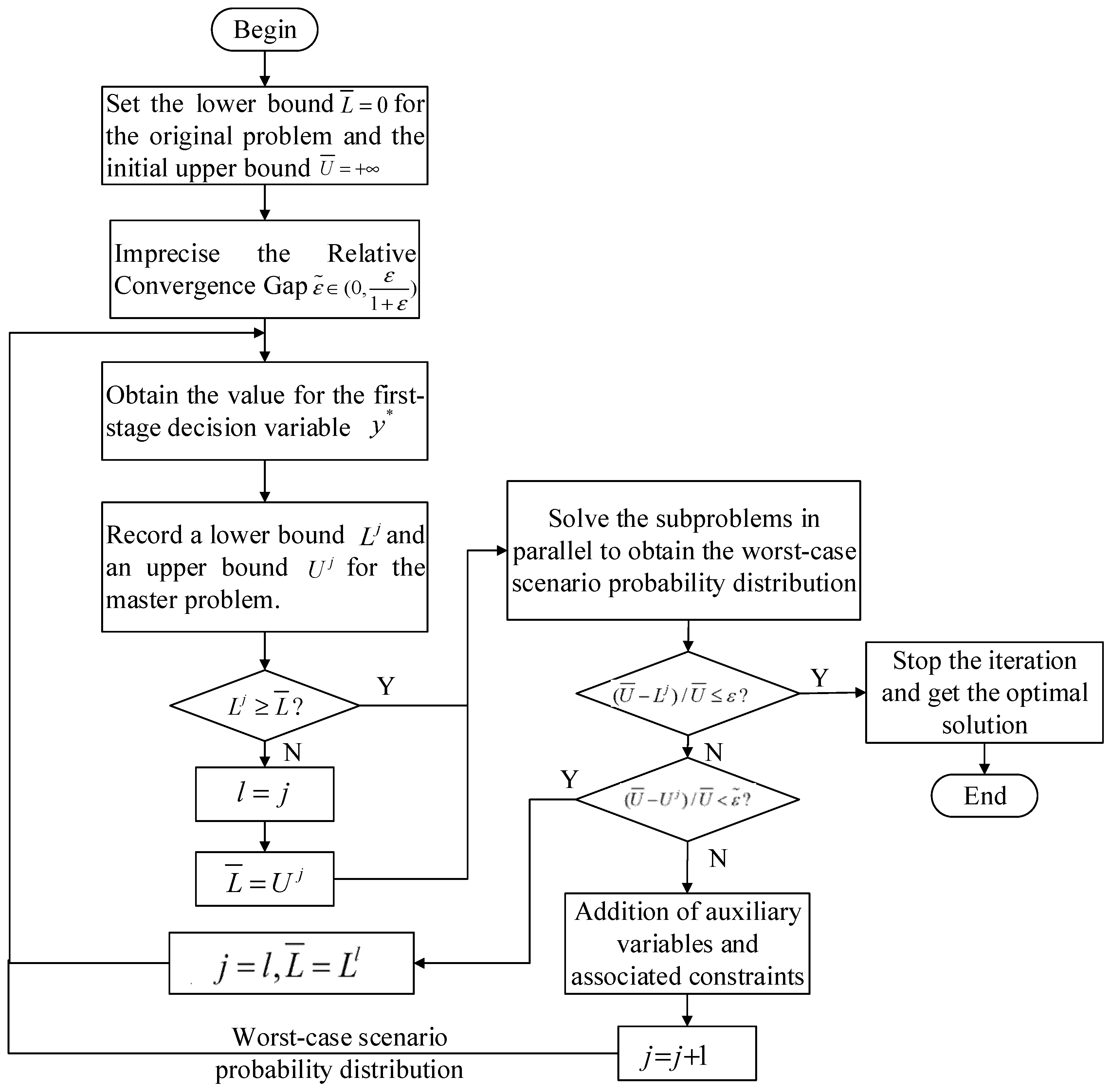
iCCG acceleration: A dynamic gap-adjustment strategy reducing iterations by 35.2% versus standard CCG, resolving convergence issues in non-convex systems.

Existing research on ADN has the following problems that need to be solved:

(1)

Uncertainty modeling dilemma: Source–load bilateral uncertainty is affected by weather, user behavior, and other factors; existing methods such as a single probability distribution assumptions cannot accurately portray its spatial and temporal correlation characteristics, resulting in significant deviation between the prediction model and the actual situation.

(2)

Multi-objective optimization contradiction: When dealing with different operating scenarios such as PV output fluctuation and demand response variations, the existing algorithms struggle to simultaneously satisfy the balance between the completeness of multi-scenario coverage and computational efficiency, as well as the synergy between robustness and economic optimization, often falling into the “over-conservative solution”. The existing algorithms often fall into the decision making dilemma of an “over-conservative solution” or “fragile optimal solution”.

In this paper, to address the difficult problem of optimal scheduling when both source-side PV output and load-side transferable load demand response are in an inexact probability distribution, firstly, a two-stage distributed robust optimization mathematical model is constructed; secondly, the solution algorithm of the corresponding two-stage distributed robust optimization model is investigated, and it is proposed to adopt the inexact columns and constraints generating the algorithm for accelerated solving of the model; finally, the proposed two-stage distribution robust optimization method is tested in the IEEE 33 distribution network with distributed power sources, PV power stations, PV plants, reactive power compensation devices, and switchable loads as an example test system to verify the effectiveness of the proposed two-stage distribution robust optimization method.

2. Robust Optimization Model for Active Distribution Grid Distribution Considering Photovoltaic Uncertainty and Demand Response

2.1. Objective Function

This study aims to synergistically cope with source–load bilateral uncertainty in active distribution networks through a two-stage distribution robust optimization framework. Specifically, the first stage takes minimizing the power purchase cost of the distribution network as the optimization objective, while the second stage focuses on the multi-objective co-optimization under the worst probability distribution scenario of the PV output, covering the integrated minimization of network active loss, distributed power generation cost, PV abandonment penalty, and transferable load compensation cost. The overall optimization objective function can be expressed as the following two-layer structure:

$$\min \left\{C_{op}+\underset{p_s\in {\mathrm{\Omega }}_p}{\max }\min E_p\left(P_{loss}+C_{DG}+C_{PV}+C_{DR}\right)\right\}$$

(1)

$$C_{op}={\displaystyle \sum _{t\in T}{C}_{gd}{P}_{j,t}^{gd}}$$

(2)

$$P_{loss}={\displaystyle \sum _{t\in T}{\displaystyle \sum _{(i,j)\in N_{DN}}{I}_{ij,t}^2{r}_{ij}}}$$

(3)

$$C_{DG}={\displaystyle \sum _{t\in T}{\displaystyle \sum _{j\in N_{DG}}\left(c_{dg}{P}_{j,t}^{dg}\right)}}$$

(4)

$$C_{PV}=c_{pv}{\displaystyle \sum _{t\in T}{\displaystyle \sum _{j\in N_{PV}}({\tilde{P}}_{j,t}^{PV}-P_{j,t}^{PV})}}$$

(5)

$$C_{DR}=c_{dr}{\displaystyle \sum _{t\in T}{\displaystyle \sum _j\left|P_{j,t}^{\mathrm{dr}}-P_{j,t}^{ld}\right|}}$$

(6)

where the subscript t represents the index of the time period; the subscript j represents the index of the node.

This two-stage objective function aims to achieve a balance between economics and robustness by synergistically optimizing the power purchase cost (first stage) with multiple objectives such as network loss and a penalty for abandoned light (second stage). The effectiveness of this design is verified by comparing the operating costs of different methods in the case study analysis later.

2.2. Constraints

In the two-stage distribution robust optimization model taking into account the source-side PV uncertainty and load-side demand response, the constraints include the distribution network’s current constraints, the distribution network node voltage constraints, the SVG reactive output constraints, the distribution network line current constraints, the distributed PV active and reactive output upper and lower limit constraints, the DG active and reactive output upper and lower limit constraints, the load constraints on demand response, and the distributed PV output uncertainty set.

The details are described as follows:

(1)

Current constraints for Distflow-based power flow modeling:

$${\displaystyle \sum _{j\in \phi \left(i\right)}\left(P_{ij,t}-r_{ij}{I}_{ij,t}^2\right)+P_{i,t}}={\displaystyle \sum _{k\in \nu \left(i\right)}{P}_{ik,t}}$$

(7)

$${\displaystyle \sum _{j\in \phi \left(i\right)}\left(Q_{ij,t}-x_{ij}{I}_{ij,t}^2\right)+Q_{i,t}}={\displaystyle \sum _{k\in \nu \left(i\right)}{Q}_{ik,t}}$$

(8)

$$V_{i,t}^2=V_{j,t}^2-2\left(r_{ij}{P}_{ij,t}+x_{ij}{Q}_{ij,t}\right)+(r_{ij}^2+x_{ij}^2)I_{ij,t}^2$$

(9)

$$P_{ij,t}^2+Q_{ij,t}^2=I_{ij,t}^2{V}_{i,t}^2$$

(10)

$$P_{i,t}=P_{i,t}^{gd}+P_{i,t}^{dg}+P_{i,t}^{PV}-P_{i,t}^{dr}$$

(11)

$$Q_{i,t}=Q_{i,t}^{dg}+Q_{i,t}^{PV}+Q_{i,t}^{SVC}-Q_{i,t}^{ld}$$

(12)

(2)

Distribution network node voltage constraints:

$$V_{i,\min }\le V_{i,t}\le V_{i,\max }$$

(13)

(3)

SVG reactive power output constraints:

$$Q_{i,\min }^{SVG}\le Q_{i,t}^{SVG}\le Q_{i,\max }^{SVG}$$

(14)

(4)

Distribution network line current constraints:

$$I_{ij,t}^2\le I_{ij,\max }^2$$

(15)

(5)

Upper and lower constraints on active and reactive power output of PV generation:

$$0\le P_{j,t}^{PV}\le {\tilde{P}}_{j,t}^{PV}$$

(16)

$$-P_{j,t}^{PV}\tan {\theta }_{PV}\le Q_{j,t}^{PV}\le P_{j,t}^{PV}\tan {\theta }_{PV}$$

(17)

(6)

DG active and reactive output upper and lower constraints:

$$P_{j,\min }^{dg}\le P_{j,t}^{dg}\le P_{j,\max }^{dg}$$

(18)

$$Q_{j,\min }^{dg}\le Q_{j,t}^{dg}\le Q_{j,\max }^{dg}$$

(19)

(7)

Demand response load constraints

In this paper, load-side demand response is considered in source–load co-optimization, and transferable loads are mainly considered, i.e., the loads of the users in the time period of electricity consumption can be appropriately adjusted by incentives in the process of active distribution network scheduling, and the constraints that need to be satisfied by the transferable loads are as follows:

$$P_{j,\min }^{dr}\le P_{j,t}^{\mathrm{dr}}\le P_{j,\max }^{dr}$$

(20)

$${\displaystyle \sum _{t\in T}{P}_{j,t}^{\mathrm{dr}}}={\displaystyle \sum _{t\in T}{P}_{i,t}^{ld}}$$

(21)

$${\displaystyle \sum _{t\in T}{\gamma }_{state}\ge T_{\min }^{ld}[P_{j,t}^{dr}(t)-P_{j,t}^{dr}(t-1)]}$$

(22)

(8)

Distributed PV Output Uncertainty Set

Based on the 1-parameter and ∞-parameter constraints to model the uncertainty of photovoltaic power generation, fuzzy sets describing the uncertainty of the probability distribution of the scenarios are constructed according to the typical scenarios, which are expressed in the following formulas [23]:

$$0\le p_s\le 1$$

(23)

$${\displaystyle \sum _{s=1}^{N_s}{p}_s}=1$$

(24)

$${\displaystyle \sum _{s=1}^{N_s}\left|p_s-p_s^0\right|\le {\theta }_1}$$

(25)

$$\underset{1\le s\le N_s}{\max }\left|p_s-p_s^0\right|\le {\theta }_{\infty }$$

(26)

Since there is an error between the initial probability distribution obtained through scene aggregation and the actual distribution, the error of the typical scene probability distribution obtained based on the aggregation of historical scenes should satisfy the following confidence interval [24]:

$$\mathrm{Pr}\left\{{\displaystyle \sum _{s=1}^{N_s}\left|p_s-p_s^0\right|\le {\theta }_1}\right\}\ge {\alpha }_1$$

(27)

$$\mathrm{Pr}\left\{\underset{1\le s\le N_s}{\max }\left|p_s-p_s^0\right|\le {\theta }_{\infty }\right\}\ge {\alpha }_{\infty }$$

(28)

$${\theta }_1={\displaystyle \frac{N_s}{2M_s}}\ln {\displaystyle \frac{2N_s}{1-{\alpha }_1}}$$

(29)

$${\theta }_{\infty }={\displaystyle \frac{1}{2M_s}}\ln {\displaystyle \frac{2N_s}{1-{\alpha }_{\infty }}}$$

(30)

where Pr{ } denotes the probability; ${\alpha }_1$ and ${\alpha }_{\infty }$ is the confidence level.

In the distributional robust optimization framework, the selection of the confidence interval (α₁, α_∞) directly affects the conservatism of the probabilistic fuzzy set Ω_p through Equations (28) and (29), which in turn acts on the two-stage optimization results.

3. Model Transformation Considering New Energy Output Uncertainty

Since the model constructed in the previous section is a nonlinear model in which there is a square term $r_{ij}{I}_{ij,t}^2$ in the objective function Equation (3), there are square terms $r_{ij}{I}_{ij,t}^2$, $V_{i,t}^2$, and $V_{j,t}^2$ in the power flow constraints Equation (7) to Equation (9), there is an absolute value term $\left|p_s-p_s^0\right|$ in the uncertainty set of distributed PV output Equations (24) and (25), and there is an absolute value term $\left|P_{j,t}^{\mathrm{dr}}-P_{j,t}^{ld}\right|$ in the objective function Equation (6), it is difficult to directly solve the model containing the above nonlinear terms.

Nonlinear term $I_{ij,t}^2={\displaystyle \frac{P_{ij,t}^2+Q_{ij,t}^2}{V_{i,t}^2}}$ in the power flow equation leads to nonconvex models. By introducing auxiliary variables ${\tilde{I}}_{ij,t}=I_{ij,t}^2$ and ${\tilde{V}}_{ij,t}=V_{ij,t}^2$, the original equation constraints can be relaxed to inequalities ${\tilde{I}}_{ij,t}{\tilde{V}}_{ij,t}\ge P_{ij,t}^2+Q_{ij,t}^2$, and Equation (32) can be transformed into the standard second-order cone form:

$${‖\begin{array}{c}2P_{ij,t}\\ 2Q_{ij,t}\\ {\tilde{I}}_{ij,t}-{\tilde{V}}_{i,t}\end{array}‖}_2⩽{\tilde{I}}_{ij,t}+{\tilde{V}}_{i,t}$$

(31)

Therefore, the distribution network current constraints Equations (7) through (10) can be rewritten as

$${\displaystyle \sum _{j\in \phi \left(i\right)}\left(P_{ij,t}-{\tilde{I}}_{ij,t}{r}_{ij}\right)+P_{i,t}}={\displaystyle \sum _{k\in \nu \left(i\right)}{P}_{ik,t}}$$

(32)

$${\displaystyle \sum _{j\in \phi \left(i\right)}\left(Q_{ij,t}-{\tilde{I}}_{ij,t}{x}_{ij}\right)+Q_{i,t}}={\displaystyle \sum _{k\in \nu \left(i\right)}{Q}_{ik,t}}$$

(33)

$${\tilde{V}}_{i,t}={\tilde{V}}_{j,t}-2\left(r_{ij}{P}_{ij,t}+x_{ij}{Q}_{ij,t}\right)+(r_{ij}^2+x_{ij}^2){\tilde{I}}_{ij,t}$$

(34)

$${‖\begin{array}{c}2P_{ij,t}\\ 2Q_{ij,t}\\ {\tilde{I}}_{ij,t}-{\tilde{V}}_{i,t}\end{array}‖}_2⩽{\tilde{I}}_{ij,t}+{\tilde{V}}_{i,t}$$

(35)

Accordingly, the objective function term (3), the node voltage constraint (13), and the line current constraint (15) can be rewritten as follows, respectively:

$$P_{loss}={\displaystyle \sum _{t\in T}{\displaystyle \sum _{(i,j)\in N_{DN}}{\tilde{I}}_{ij,t}{r}_{ij}}}$$

(36)

$$V_{i,\min }^2\le {\tilde{V}}_{i,t}\le V_{i,\max }^2$$

(37)

$${\tilde{I}}_{ij,t}\le I_{ij,\max }^2$$

(38)

3.1. Linearization of Uncertainty Fuzzy Sets

Since the distributed PV output uncertainty fuzzy sets Equation (24) to Equation (25) appear as absolute value terms, which are nonlinear constraints, this study introduces auxiliary variables and uses the large M method to transform the absolute value constraints Equation (24) to Equation (25) to linear constraints containing 0–1 variables, which change as follows:

$$0\le p_s^{+}\le {\sigma }_s^{+}{\theta }_1$$

(39)

$$0\le p_s^{-}\le {\sigma }_s^{-}{\theta }_1$$

(40)

$${\sigma }_s^{+}+{\sigma }_s^{-}\le 1$$

(41)

$${\displaystyle \sum _{s=1}^{N_s}\left(p_s^{+}+p_s^{-}\right)\le {\theta }_1}$$

(42)

$$p_s^{+}+p_s^{-}\le {\theta }_{\infty }$$

(43)

$$\left|p_s-p_s^0\right|=p_s^{+}+p_s^{-}$$

(44)

$$p_s-p_s^0=p_s^{+}-p_s^{-}$$

(45)

where $p_s^{+}$ and $p_s^{-}$ are non-negative auxiliary variables indicating the amount of positive and negative deviation of the actual probability of the sth scenario from the initial probability, respectively; ${\sigma }_s^{+}$ and ${\sigma }_s^{-}$ are 0–1 auxiliary variables.

The distributed PV output uncertainty fuzzy set is then transformed into the following linear constraint:

$${\mathrm{\Omega }}_p=\left\{\begin{array}{l}0\le p_s\le 1\\ {\displaystyle \sum _{s=1}^{N_s}{p}_s}=1\\ {\displaystyle \sum _{s=1}^{N_s}\left(p_s^{+}+p_s^{-}\right)\le {\theta }_1}\\ p_s^{+}+p_s^{-}\le {\theta }_{\infty }\\ 0\le p_s^{+}\le {\sigma }_s^{+}{\theta }_1\\ 0\le p_s^{-}\le {\sigma }_s^{-}{\theta }_1\\ {\sigma }_s^{+}+{\sigma }_s^{-}\le 1\\ p_s-p_s^0=p_s^{+}-p_s^{-}\end{array}\right.$$

(46)

3.2. Linearization of Absolute Value Terms in Objective Functions

Since the absolute value term appears in the objective function term Equation (6), the absolute value term $\left|P_{j,t}^{\mathrm{dr}}-P_{j,t}^{ld}\right|$ can be linearized by introducing the auxiliary variables $Z_{j,t}^{\mathrm{dr}}$, and adding the constraints Equation (50) to Equation (51), Equation (6) can be transformed into the following equivalent linearized form:

$$C_{DR}=c_{dr}{\displaystyle \sum _{t\in T}{\displaystyle \sum _j{Z}_{j,t}^{\mathrm{dr}}}}$$

(47)

$$Z_{j,t}^{\mathrm{dr}}\ge P_{j,t}^{\mathrm{dr}}-P_{j,t}^{ld}$$

(48)

$$Z_{j,t}^{\mathrm{dr}}\ge P_{j,t}^{ld}-P_{j,t}^{\mathrm{dr}}$$

(49)

4. Algorithms for Solving Two-Stage Distributional Robust Optimization Models

For the two-stage distribution robust optimization model constructed above, the traditional method uses the column-and-constraint generation (CCG) algorithm to solve the model, which adds variables and constraints to the master problem when solving the master problem and subproblems alternately [25,26,27]. Considering the auxiliary variables and constraints introduced by linearization in the model constructed in this paper, a large number of variables and constraints will be added to the main problem in each iteration when solving the model using the CCG algorithm, and the scale of the main problem will increase as it iterates, which will increase the difficulty of solving it [28,29]. Therefore, this paper adopts the inexact column-and-constraint generation (iCCG) algorithm to solve the model constructed in this paper, and the idea of this algorithm is to sacrifice the accuracy of the main problem to achieve a fast solution. Non-exact variables are added in the loop iteration process, which is equivalent to adding a new buffer layer in the traditional CCG algorithm, the current solution state is recognized, and different solution states will enter different solution stages until the algorithm converges. A proof of convergence of the iGGC algorithm can be found in Appendix A.

In order to conveniently illustrate the idea of the iCCG algorithm, the above two-stage distribution robust optimization model is rewritten in the following compact form:

$$\left\{\begin{array}{l}\underset{\mathrm{y}}{\min }{\mathit{a}}^T\mathrm{y}+\underset{p_s\in {\Omega }_p}{\max } \underset{{\mathrm{x}}_s}{\min }{\displaystyle \sum _{s=1}^{N_s}{p}_s}{\mathit{b}}^T{\mathrm{x}}_s\\ \mathrm{s}.\mathrm{t}.\mathit{C}\mathrm{y}\le \mathit{c}\\ \mathit{D}\mathrm{y}=\mathit{d}\\ \mathit{E}{\mathit{x}}_s\le \mathit{e}\\ \mathit{F}{\mathit{x}}_s=\mathit{f}\\ \mathit{G}\mathit{y}+\mathit{H}{\mathit{x}}_s\le \mathit{g}\\ \mathit{J}\mathit{y}+\mathit{K}{\mathit{x}}_s=\mathit{h}\\ {‖\mathit{L}{\mathit{x}}_s‖}_2\le {\mathit{m}}^T{\mathit{x}}_s\end{array}\right.$$

(50)

where y is the vector of decision variables in stage 1; x_s is the vector of stage 2 variables in the sth scenario; a and b denote the cost coefficient matrices of stage 1 and stage 2 variables, respectively; and C, D, E, F, G, H, J, K, L, c, d, e, f, g, h, and m are the corresponding coefficient matrices.

The above two-stage distributional robust optimization model can be decomposed into a master problem and a subproblem, where the master problem can be written in the following form:

$$\left\{\begin{array}{l}\mathrm{MP}:\underset{y,x_{s,l}}{\min } {\mathit{a}}^T\mathit{y}+\eta \\ \mathrm{s}.\mathrm{t}.\mathit{C}\mathrm{y}\le \mathit{c}\\ \mathit{D}\mathrm{y}=\mathit{d}\\ \eta \ge {\displaystyle \sum _{s=1}^{N_s}{p}_{s,l}^{*}}{\mathit{b}}^T{\mathrm{x}}_{s,l},l=1,2,\dots ,r\\ \mathit{G}\mathit{y}+\mathit{H}{\mathrm{x}}_{s,l}\le \mathit{g},l=1,2,\dots ,r;s=1,2,\dots ,N_s\\ \mathit{J}\mathit{y}+\mathit{K}{\mathrm{x}}_{s,l}=\mathit{h},l=1,2,\dots ,r;s=1,2,\dots ,N_s\\ {\mathit{a}}^T\mathit{y}+\eta \ge \overline{L}\end{array}\right.$$

(51)

where l denotes the number of iterations; x_s,l denotes the auxiliary variable generated in the main problem at the lth iteration related to the subproblem; $p_{s,l}^{*}$ is the worst-case scenario probability of PV outflow obtained by solving the subproblem at the lth iteration, and this parameter is a known quantity when solving the main problem; η is the relaxation of the objective function value of the second stage; and $\overline{L}$ denotes the lower bound of the optimal objective of the main problem.

The subproblem can be written in the following form:

$$\left\{\begin{array}{l}\mathrm{SP}:\underset{p_s\in {\Omega }_p}{\max } \underset{x_s}{\min }{\displaystyle \sum _{s=1}^{N_s}{p}_s}{\mathit{b}}^T{\mathit{x}}_s\\ \mathrm{s.t.} \mathit{E}{\mathit{x}}_s\le \mathit{e}\\ \mathit{F}{\mathit{x}}_s=\mathit{f}\\ \mathit{G}{\mathit{y}}^{*}+\mathit{H}{\mathit{x}}_s\le \mathit{g}\\ \mathit{J}{\mathit{y}}^{*}+\mathit{K}{\mathit{x}}_s=\mathit{h}\\ {‖\mathit{L}{\mathit{x}}_s‖}_2\le {\mathit{m}}^T{\mathit{x}}_s\end{array}\right.$$

(52)

where y* is the solution to the master problem, passed as a parameter to the subproblem, and it is a known quantity when solving the subproblem.

The subproblem is a max–min two-layer optimization problem, and since the decision variable p_s in the outer layer and the decision variable x_s in the inner layer are independent of each other, the subproblem can be further decomposed into two single-layer problems for solving the inner min problem first and then the outer max problem, where the inner min problems in each scenario are independent of each other and can be solved in parallel. The subproblem is transformed into two single-layer problems as follows:

Inner layer min issues:

$$\left\{\begin{array}{l}{\varphi }_s({\mathit{x}}_s)=\underset{x_s}{\min } {\mathit{b}}^T{x}_s\\ \mathrm{s}.\mathrm{t}.\mathit{E}{\mathit{x}}_s\le \mathit{e}\\ \mathit{F}{\mathit{x}}_s=\mathit{f}\\ \mathit{G}{\mathit{y}}^{*}+\mathit{H}{\mathit{x}}_s\le \mathit{g}\\ \mathit{J}{\mathit{y}}^{*}+\mathit{K}{\mathit{x}}_s=\mathit{h}\\ {‖\mathit{L}{\mathit{x}}_s‖}_2\le {\mathit{m}}^T{\mathit{x}}_s\end{array}\right.$$

(53)

Outer max issues:

$$\left\{\begin{array}{l}\underset{p_s}{\max }{\displaystyle \sum _{s=1}^{N_s}{p}_s}{\varphi }_s({\mathit{x}}_s^{*})\\ \mathrm{s}.\mathrm{t}. p_s\in {\Omega }_p\end{array}\right.$$

(54)

where ${\varphi }_s({\mathit{x}}_s)$ denotes the objective function of the inner min problem for the sth distributed PV outflow scenario, and the objective function ${\varphi }_s({\mathit{x}}_s^{*})$ of the inner min problem is the objective function value which is fixed in the solution process of the outer max problem, which is a known parameter.

The decomposition of SP is based on the following mathematical properties: since the inner optimization variable x_s is uncoupled from the outer probability distribution p_s and the outer objective is linear with respect to p_s, according to the strong duality and the dyadic theory of linear programming, the max–min structure can be equivalently decomposed into two layers of independent optimization problems. The inner min problem can be decoupled to each scenario and solved in parallel, which significantly improves computational efficiency.

Unlike the CCG algorithm that solves the two-stage distributional robust optimization model alternatively, the iCCG algorithm first solves the master problem with a relative optimal gap and adds an additional constraint equation that reduces the time for exploring the optimal solution by setting a tight lower bound, which is obtained by solving the master problem Equation (53) with the lower and upper bounds of the master problem, as well as the first-stage decision variable y optimal solution. Then, the obtained values of the first-stage decision variables are passed as parameters to the subproblems, and the subproblems are solved with the first-stage variable y* fixed; the worst-case scenario probability distribution $p_{s,l}^{*}$ is obtained by solving the inner min problems of the subproblems in parallel, and the outer max problems of the subproblems are solved to obtain the upper bounds of Equation (52). At this time, it is necessary to judge the gap relationship between the upper bound of Equation (52) and the upper bound of the master problem. If it is smaller than the inexact relative convergence gap, it is necessary to re-solve the master problem and update the relative optimal gap of the master problem to a smaller value; if the gap is larger than the inexact relative convergence gap, pass the worst-case scenario probability distribution $p_{s,l}^{*}$ as a parameter to the master problem and add Equation (53) as a cut-plane constraint added to the master problem. Until the difference between the upper and lower bounds of the objective function values during the iteration process meets the convergence requirements, the iterative computation is stopped.

In a later analysis of the case, we will compare the results of different optimization methods.

In summary, the two-stage distribution robust optimization process based on the iCCG algorithm can be summarized as shown in Figure 1.

5. Case Analysis

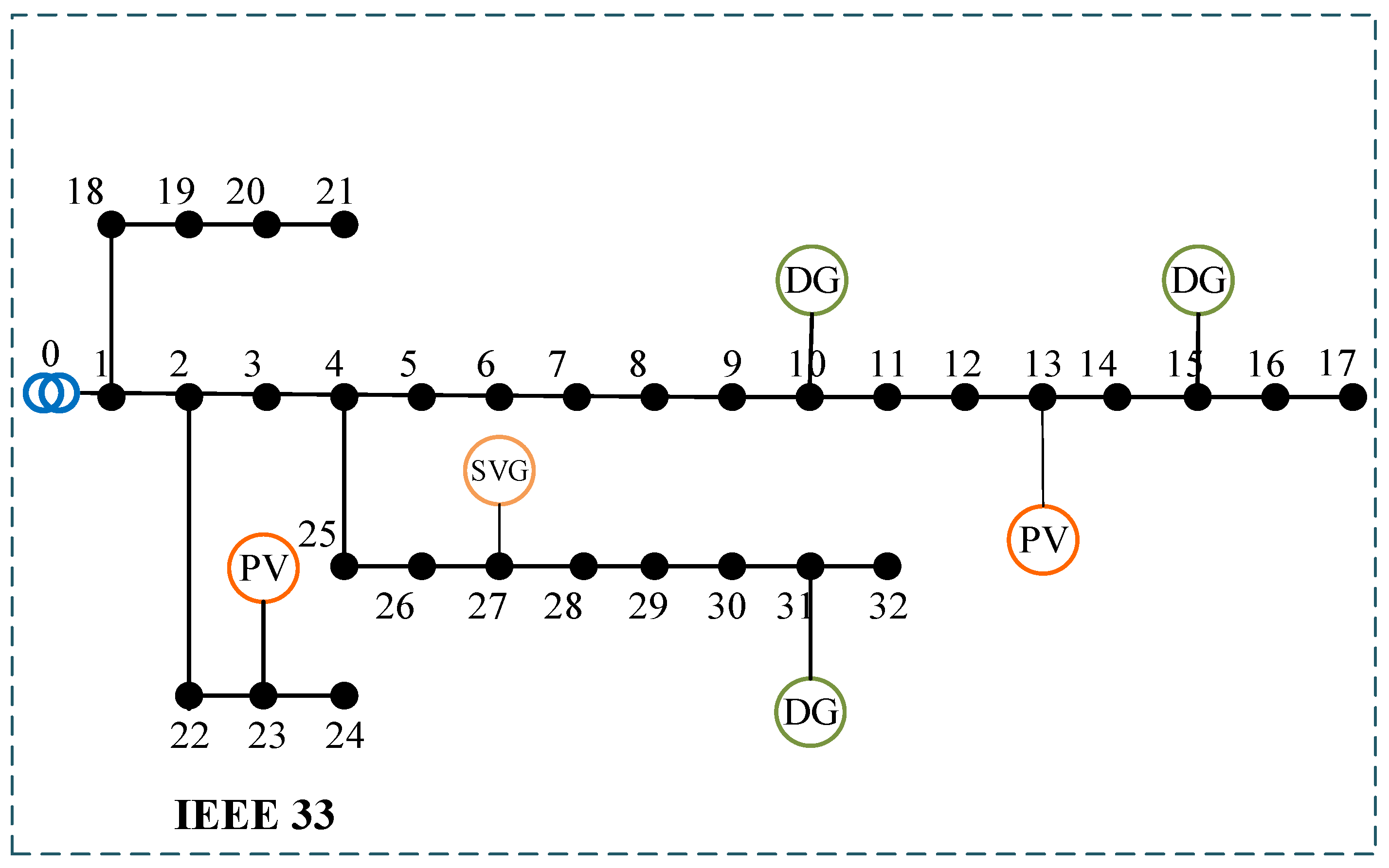
5.1. Parameterization

In this study, a modified IEEE 33 bus active distribution network is used as a test system to validate the effectiveness of the proposed two-stage distribution robust optimization method. The topology of the distribution system is shown in Figure 2, in which distributed energy sources are connected at distribution nodes 10, 15, and node 31, the maximum capacity of each DG is 1.3 MW, the cost of power generation is USD 170/MW for each DG, and the power factor is 0.85. A PV plant is installed at node 13 and node 23, with a maximum installed capacity of 1.8 MW and a power factor of 0.9. The active power prediction error of the PV plant is 15%, and the PV power abandonment penalty cost coefficient is USD 300/MW. The distribution network is equipped with one SVG, which is installed at node 27 and has a maximum reactive power compensation capacity of 0.8 MVar. The voltage amplitude range is 0.95 p.u. to 1.05 p.u. The distribution network also has a certain percentage of switchable load.

The convergence accuracy of the iCCG algorithm is set to 10-5 in the simulation. The computer configuration is Intel(R) Core(TM) i7-1065G7 CPU/1.30-GHz main frequency 8 GB RAM. The proposed algorithm is implemented in the MATLAB 2022a environment and the commercial solver CPLEX 12.10 is called for solving.

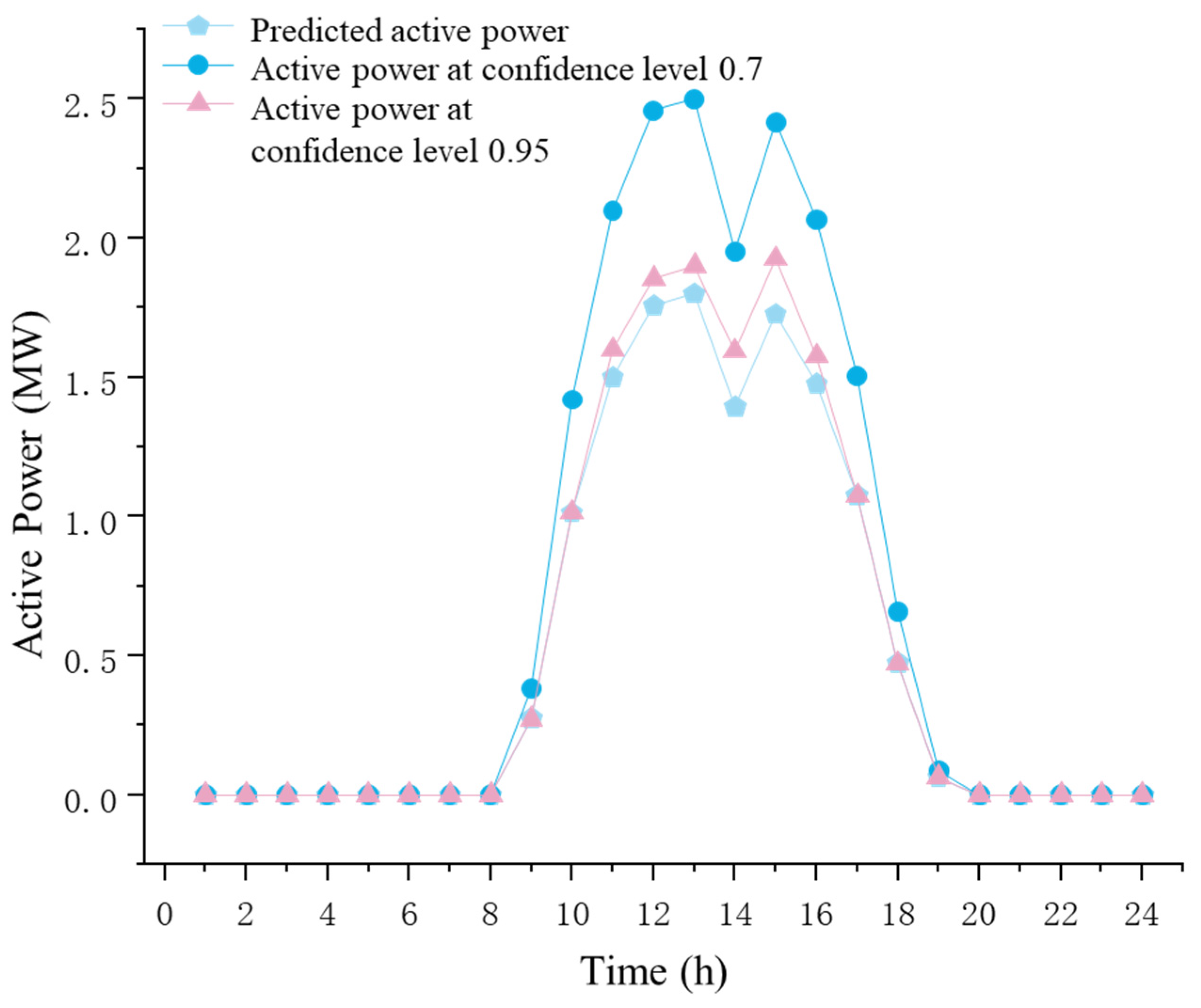
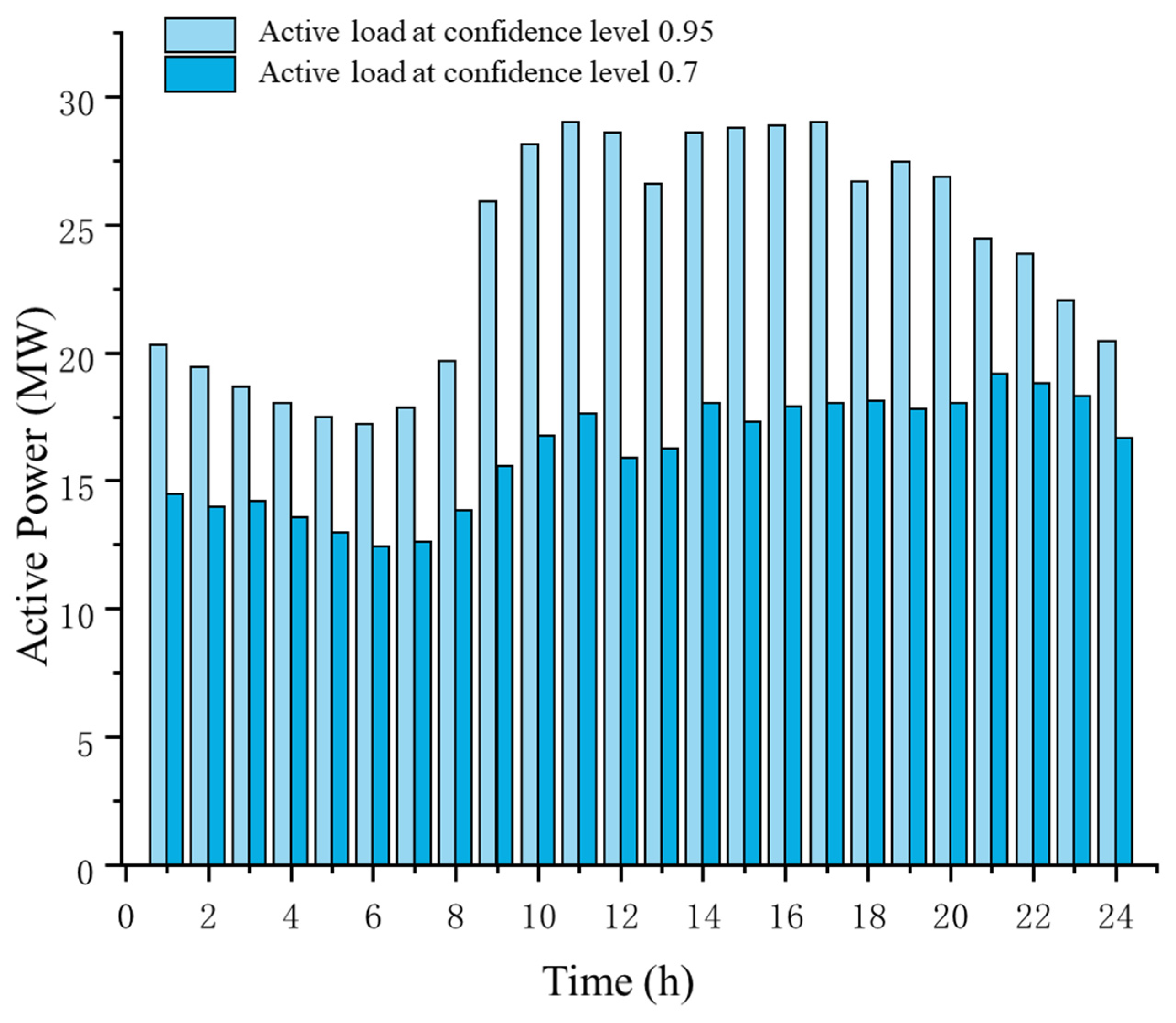
5.2. Simulation Results and Analysis

Figure 3 shows the results of the active power prediction of PV power generation, from which the active power output of PV power generation under the uncertainty confidence level of different probability density functions can be seen. As the uncertainty confidence level continues to increase, the volatility of the active power output of PV power generation decreases; when the confidence level is 0.7, there are 12 time periods in 24 h in which the active power of PV power generation is greater than the predicted active power, showing a greater fluctuation of PV output at a confidence level of 0.7. It shows that the PV output fluctuates more at a confidence level of 0.7; when the confidence level is 0.95, there are six periods within 24 h in which the active power of PV generation is greater than the predicted active power, and the active power of PV generation in more than six periods is highly volatile compared to the confidence level of 0.7. This indicates that as the confidence level increases, the active output of PV power generation tends to be relatively stable.

Figure 4 shows the load-shedding capacity under different uncertainty confidence levels, from which it can be seen that the system cut-load capacity decreases as the uncertainty confidence level increases, which also means that the more stable the active output of PV power generation, the less impact on the system cut-load. Moreover, during the 9–17 time period, the load is relatively high, and the active load is much higher when the confidence level is 0.95 than when the confidence level is 0.7, which indicates that when the uncertainty of the PV power generation is very strong as the confidence level decreases, it will lead to an increase in the cut-load capacity.

The impact of the uncertainty of PV power generation on the operating cost of the distribution grid at different uncertainty confidence levels is given in

Table 1. Comparison of operating costs for different uncertainty confidence levels.

Sample Size	Running Cost at Confidence Level of 0.65 (CNY)	Running Cost at Confidence Level of 0.70 (CNY)	Running Cost at Confidence Level of 0.95 (CNY)
10,000	52,694.3	52,987.5	53,210.7
5000	52,784.1	53,037.2	53,789.7
1000	55,278.8	55,278.6	55,278.9

. From Table 1, it can be seen that when the uncertainty confidence level of PV power generation is certain, the operating cost of the distribution network increases with the decrease in the number of samples, and the operating cost of the distribution network reaches the maximum when the number of samples is 1000. At the same time, when the number of samples is certain, as the confidence level continues to increase, the operating cost of the distribution network is also increasing; this is because as the confidence level increases, the output of PV power generation tends to stabilize, and at the same time, the cut-load capacity of the distribution network decreases, which will lead to a trend in increasing the operating cost of the distribution network.

A comparison of the results of stochastic optimization, robust optimization, and distributional robust optimization is given in

Table 2. Comparison of system operating costs under different optimization methods.

Optimization Methods	Operating Costs of the Distribution Network (CNY)	Robustness (Cut-Load in Peak Hour)
Stochastic optimization methods	53,822.7	α = 0.7, load cutting 4.8 MW
Robust optimization methods	58,647.1	load cutting 0 MW
Distributed robust optimization methods	55,278.8	α = 0.95, load cutting 1.2 MW

. In this case, the number of samples under the distribution robust optimization method is chosen to be 1000, and the PV power generation uncertainty confidence level is chosen to be 0.95.

As can be seen from

Table 3. Convergence time (s) and improvement rate (%) of iCCG algorithm with different parameters.

${\mathit{\epsilon }}_{\mathit{M}\mathit{P}}$	iCCG Algorithm						CCG Algorithm
	$\tilde{\mathit{\epsilon }}=\mathit{\epsilon }/(2(1+\mathit{\epsilon }))$			$\tilde{\mathit{\epsilon }}=\mathit{\epsilon }/(1+\mathit{\epsilon })$
	$\mathit{\lambda }=0.2$	$\mathit{\lambda }=0.5$	$\mathit{\lambda }=0.8$	$\mathit{\lambda }=0.2$	$\mathit{\lambda }=0.5$	$\mathit{\lambda }=0.8$
10−1	701.67 s	755.18 s	780.67 s	672.59 s	731.56 s	733.71 s	782.38 s
10−2	925.85 s	1027.32 s	115.45 s	926.14 s	970.87 s	985.76 s	1468.67 s
10−4	1436.65 s	1567.66 s	1675.78 s	1425.38 s	1478.65 s	1469.52 s	1735.10 s

, this study compares three optimization methods for dealing with the uncertainty of new energy sources, and the significance of the comparison is that it reveals the conservatism of the different methods in dealing with uncertainty and demonstrates the advantages of the distribution robust optimization method proposed in this study. The distributional robust optimization method proposed in this study is relatively more conservative than the results obtained by the stochastic optimization method, and its distribution network operation cost is higher than that under the stochastic optimization method by 1456.1 RMB. This is because, under the stochastic optimization method, only the results calculated by considering the empirical probability density function are taken into account, so the optimization strategy obtained is relatively more ideal and its economy is better. However, compared to the robust optimization method, this method does not consider the probability distribution of uncertainty and only considers the worst scenario of PV power output, so the optimization results obtained are the most conservative. For the distributional robust optimization method proposed in this study, the probabilistic distribution of uncertainty is taken into account and more robust results can be obtained, but the cost of the robust optimization results is more expensive compared to the stochastic optimization method within a certain range.

From the comparison of the solution time of the iCCG algorithm and the CCG algorithm under different parameters in Table 3, it can be seen that the iCCG algorithm is able to shorten the solution time within the permissible error compared to the CCG algorithm for a given algorithmic iteration permissible error. For the iCCG algorithm, the difference between the iCCG algorithm solution time and the CCG algorithm is small when the inexact relative error is small. At this time, the iCCG algorithm prefers to add new scenarios to the master problem, so the solution efficiency enhancement is limited, but when the master problem is relatively converged to gap iteration factor λ = 0.2, the solution speed enhancement is larger because at this time, the difference between the master problem solution accuracy and the algorithm solution is smaller. The smaller $\lambda$ can make the algorithm converge faster; when the relative imprecision error is large, the iCCG algorithm prefers to update the relative convergence gap MP of the master problem iteration so as to reduce the precision of the master problem iteration and accelerate the algorithm’s convergence. The smaller the $\lambda$ and ${\epsilon }_{MP}$ are, the less master problem iterations are needed and the faster the solution speed.

6. Conclusions

This study proposes a two-stage distribution robust optimization model incorporating source-side PV uncertainty and load-side demand response, aiming to synergistically optimize the active and reactive power output of distributed energy sources within the active distribution network. The main contributions and findings are summarized as follows:

• Establishment of multi-objective synergistic optimization model: The established two-stage model effectively balances economic efficiency and robustness through a hierarchical optimization structure. The first stage minimizes deterministic power purchase costs, while the second stage addresses worst-case scenario losses and compensation costs. Case studies demonstrate a 5.7% reduction in operating costs compared to traditional robust optimization methods, along with a 30% decrease in load shedding capacity at a 0.95 confidence level. This dual-layer structure successfully resolves the dilemma between solution conservatism and economic optimality.
• Propose enhanced solver algorithms: The proposed iCCG algorithm improves computational efficiency by 35.2% compared to conventional CCG methods through a dynamic adjustment of convergence gaps and inexact constraint generation. The dynamic precision control mechanism reduces redundant iterations while maintaining solution accuracy, achieving an optimal balance between computational speed and optimization quality. This advancement effectively overcomes the dimensional curse issue in multi-scenario optimization problems.
• Establishment of an uncertainty management framework: The methodology combines probabilistic distribution ambiguity sets with linearization techniques, enabling comprehensive uncertainty modeling while ensuring computational tractability. The hybrid approach provides robust performance guarantees against prediction errors without excessive conservatism.

The framework demonstrates superior performance in balancing operational efficiency, solution robustness, and computational practicality, offering a viable paradigm for modern distribution network optimization. Future extensions will explore its application in heterogeneous energy systems and cyber-physical coordination scenarios.

References

1. Manuel, A.; David, R.; Camilo, A. A Distributed Coordination Approach for Enhancing Protection System Adaptability in Active Distribution Networks. Energies 2024, 17, 4338. [Google Scholar] [CrossRef]
2. Pan, P.; Chen, G.; Shi, H.; Zha, X.; Huang, Z. Distributed Robust Optimization Method for Active Distribution Network with Variable-Speed Pumped Storage. Electronics 2024, 13, 3317. [Google Scholar] [CrossRef]
3. Ding, T.; Liu, S.; Yuan, W.; Bie, Z.; Zeng, B. A Two-Stage Robust Reactive Power Optimization Considering Uncertain Wind Power Integration in Active Distribution Networks. IEEE Trans. Sustain. Energy 2016, 7, 301–311. [Google Scholar] [CrossRef]
4. Zhang, Y.; Zhang, J.; Wu, G.; Zheng, J.; Liu, D.; An, Y. Optimal Power Dispatch of Active Distribution Network and P2P Energy Trading Based on Soft Actor-critic Algorithm Incorporating Distributed Trading Control. J. Mod. Power Syst. Clean Energy 2025, 13, 540–551. [Google Scholar] [CrossRef]
5. Park, B.; Chen, Y.; Olama, M.; Kuruganti, T.; Dong, J.; Wang, X.; Li, F. Optimal Demand Response Incorporating Distribution LMP with PV Generation Uncertainty. IEEE Trans. Power Syst. 2022, 37, 982–995. [Google Scholar] [CrossRef]
6. Nikoobakht, A.; Zeraati, S.; Honkapuro, S.; Afrasiabi, M.; Aghaei, J. Toward Robust Decentralized Linear AC Operation of Cooperative Transmission and Distribution Networks. IEEE Access 2022, 10, 72603–72614. [Google Scholar] [CrossRef]
7. Rayati, M.; Bozorg, M.; Cherkaoui, R.; Carpita, M. Distributionally Robust Chance Constrained Optimization for Providing Flexibility in an Active Distribution Network. IEEE Trans. Smart Grid 2022, 13, 2920–2934. [Google Scholar] [CrossRef]
8. Zongxiang, L.U.; Yisha, L.I.N.; Ying, Q.I.A.O. Flexibility supply demand balance in power system with ultra-high proportion of renewable energy. Autom. Electr. Power Syst. 2022, 46, 3–16. [Google Scholar]
9. Tao, A.; Zhou, N.; Chi, Y.; Wang, Q.; Dong, G. Multi-stage Coordinated Robust Optimization for Soft Open Point Allocation in Active Distribution Networks with PV. J. Mod. Power Syst. Clean Energy 2023, 11, 1553–1563. [Google Scholar] [CrossRef]
10. Kalantar-Neyestanaki, M.; Sossan, F.; Bozorg, M.; Cherkaoui, R. Characterizing the Reserve Provision Capability Area of Active Distribution Networks: A Linear Robust Optimization Method. IEEE Trans. Smart Grid 2020, 11, 2464–2475. [Google Scholar] [CrossRef]
11. Cui, Z.; Bai, X.; Li, P.; Li, B.; Cheng, J.; Su, X.; Zheng, Y. Optimal strategies for distribution network reconfiguration considering uncertain wind power. CSEE J. Power Energy Syst. 2020, 6, 662–671. [Google Scholar]
12. Sepúlveda, J.; Angulo, A.; Mancilla-David, F.; Street, A. Robust Co-Optimization of Droop and Affine Policy Parameters in Active Distribution Systems with High Penetration of Photovoltaic Generation. IEEE Trans. Smart Grid 2022, 13, 4355–4366. [Google Scholar] [CrossRef]
13. Hu, W.; Wang, P.; Gooi, H. Toward Optimal Energy Management of Microgrids via Robust Two-Stage Optimization. IEEE Trans. Smart Grid 2018, 9, 1161–1174. [Google Scholar] [CrossRef]
14. Barhagh, S.S.; Mohammadi-Ivatloo, B.; Abapour, M.; Shafie-Khah, M. Optimal Sizing and Siting of Electric Vehicle Charging Stations in Distribution Networks With Robust Optimizing Model. IEEE Trans. Intell. Transp. Syst. 2024, 25, 4314–4325. [Google Scholar] [CrossRef]
15. Luo, J.; Zhang, W.; Wang, H.; Wei, W.; He, J. Research on Data-Driven Optimal Scheduling of Power System. Energies. 2023, 16, 2926. [Google Scholar] [CrossRef]
16. Park, J.Y.; Ban, J.; Kim, Y.J.; Catalão, J.P. Supplementary Feedforward Voltage Control in a Reconfigurable Distribution Network using Robust Optimization. IEEE Trans. Power Syst. 2022, 37, 4385–4399. [Google Scholar] [CrossRef]
17. Chen, Y.; Wei, W.; Liu, F.; Mei, S. Distributionally robust hydro-thermal-wind economic dispatch. Appl. Energy 2016, 173, 511–519. [Google Scholar] [CrossRef]
18. Wang, J.; Bian, Y.; Xu, Q.; Kong, X. Distributional robust optimal dispatching of microgrid considering risk and carbon trading mechanism. High Volt. Eng. 2023, 49, 1–12. [Google Scholar]
19. Zhang, J.; Cui, M.; He, Y.; Li, F. Multi-period Two-stage Robust Optimization of Radial Distribution System with Cables Considering Time-of-use Price. J. Mod. Power Syst. Clean Energy 2023, 11, 312–323. [Google Scholar] [CrossRef]
20. Zhang, K.; Wang, X.; Yang, H.; Jiang, C. Distributionally Robust Optimal Scheduling Method for Power System Under Flexibility Boundaries of Data Center Clusters. Automation of Electric Power Systems. 2024, 7, 235–247. [Google Scholar]
21. Xuan, A.; Sun, Y.; Liu, Z.; Zheng, P.; Peng, W. An ADMM-based tripartite distributed planning approach in integrated electricity and natural gas system. Appl. Energy 2025, 338, 125660. [Google Scholar] [CrossRef]
22. Lv, Q.; Wang, L.; Li, Z.; Song, W.; Bu, F.; Wang, L. Robust optimization for integrated production and energy scheduling in low-carbon factories with captive power plants under decision-dependent uncertainty. Appl. Energy 2025, 379, 124827. [Google Scholar] [CrossRef]
23. Peyman, M.; Daniel, K. Data-driven distributionally robust optimization using the Wasserstein metric: Performance guarantees and tractable reformulations. Math. Program. 2017, 171, 115–166. [Google Scholar]
24. Nicolas, F.; Arnaud, G. On the rate of convergence in Wasserstein distance of the empirical measure. Probab. Theory Relat. Fields 2014, 162, 707–738. [Google Scholar]
25. Yazdani, D.; Omidvar, M.N.; Yazdani, D.; Branke, J.; Nguyen, T.T.; Gandomi, A.H.; Jin, Y.; Yao, X. Robust Optimization Over Time: A Critical Review. IEEE Trans. Evol. Comput. 2024, 28, 1265–1285. [Google Scholar] [CrossRef]
26. Han, C.; Rao, R.R.; Cho, S. Stochastic Operation of Multi-Terminal Soft Open Points in Distribution Networks with Distributionally Robust Chance-Constrained Optimization. IEEE Trans. Sustain. Energy 2025, 16, 81–94. [Google Scholar] [CrossRef]
27. Xiang, Y.; Xue, P.; Wang, Y.; Xu, L.; Ma, W.; Shafie-Khah, M.; Li, J.; Liu, J. Robust Expansion Planning of Electric Vehicle Charging System and Distribution Networks. CSEE J. Power Energy Syst. 2024, 10, 2457–2469. [Google Scholar]
28. Nasiri, N.; Zeynali, S.; Ravadanegh, S.N.; Kubler, S. Moment-Based Distributionally Robust Peer-to-Peer Transactive Energy Trading Framework Between Networked Microgrids, Smart Parking Lots and Electricity Distribution Network. IEEE Trans. Smart Grid 2024, 15, 1965–1977. [Google Scholar] [CrossRef]
29. Homaee, O.; Najafi, A.; Jasinski, M.; Tsaousoglou, G.; Leonowicz, Z. Coordination of Neighboring Active Distribution Networks Under Electricity Price Uncertainty Using Distributed Robust Bi-Level Programming. IEEE Trans. Sustain. Energy 2023, 14, 325–338. [Google Scholar] [CrossRef]
Figure 1. Flowchart of two-stage robust optimization based on iCCG algorithm.
Energies 18 03531 g001
Figure 2. Improved IEEE 33 distribution network topology diagram.
Energies 18 03531 g002
Figure 3. Active power of photovoltaic power generation under uncertainty confidence level.
Energies 18 03531 g003
Figure 4. Capacity of cut-load at uncertainty confidence level.
Energies 18 03531 g004