Optimizing Thermal Comfort with Adaptive Behaviours in South Australian Residential Buildings

Abstract

This study focuses on thermal comfort in residential buildings within the Iron Triangle area of South Australia, examining how indoor conditions influence residents’ comfort and adaptive behaviours. Conducted from June 2023 to February 2024 across 30 homes in Port Pirie, Port Augusta, and Whyalla, the research gathered data from 38 residents, who reported indoor comfort levels in living rooms and bedrooms. A total of 3540 responses were obtained. At the same time, the measurement of indoor conditions in the buildings was performed using a small HOBO MX1104 device. Using the Mean Thermal Sensation Vote (MTSV) concept, it was possible to determine the neutral operative temperature and temperature ranges for thermal comfort categories. According to the defined linear regression formula, the neutral temperature was 23.9 °C. In living rooms, it was slightly lower, at 23.7 °C, and in bedrooms, slightly higher, at 24.4 °C. For comparison, the neutral temperature was calculated based on the average Predicted Mean Vote (MPMV) and equal to 24.3 °C. Comparison of the regression curves showed that in terms of slope, the MPMV curve is steeper (slope 0.282) than the MTSV curve (slope 0.1726), and lies above it. Regarding the residents’ behaviour, a strong correlation was found between the operative temperature T_o and the degree of clothing I_cl in living rooms. Use of ceiling fans was also studied. A clear trend was also observed regarding window and door opening. The findings of the research can be used to inform the design and operation of residential buildings with a view to enhancing thermal comfort and energy efficiency.

1. Introduction

1.1. Overview

In many industrialized countries, a significant portion of the energy consumed in buildings is dedicated to enhancing indoor thermal comfort. This suggests that the operational phase of a building presents substantial opportunities for energy savings [1,2]. However, an indiscriminate reduction in energy consumption may compromise the quality of the indoor thermal environment. Therefore, the key challenge is to minimize energy use without diminishing residents’ quality of life. As economic conditions improve and living standards rise, people increasingly demand higher levels of comfort and well-being.

Thermal comfort within residential buildings is a critical aspect of indoor environmental quality, exerting a significant influence on the health and productivity of the occupants. This study examines the internal parameters of buildings and their perception by residents in three towns of the Iron Triangle in South Australia, with a focus on understanding the relationship between indoor conditions and comfort sensations. The concept of thermal comfort is influenced by a range of factors, including, among others, metabolic activity, insulation of clothes, air temperature, radiant temperature, humidity, and air velocity. To provide a comprehensive analysis, this study employs the concept of the Predicted Mean Vote (PMV) and the operative temperature, which is a measure combining these factors to reflect the thermal environment as experienced by residents.

High temperatures can cause occupants to experience prolonged discomfort [3], which negatively impacts human health. Therefore, field studies on the thermal environment across different climatic zones in Australia are urgently needed to establish appropriate thermal comfort assessment criteria tailored to local conditions. This research aimed to address knowledge gaps regarding actual occupant heating and cooling practices in climate zone 4 of South Australia. Additionally, it sought to examine whether homes in this climate zone are prone to overheating when cooling systems are not in use (i.e., in free-running mode). The findings will help refine occupant behaviour settings in the Nationwide House Energy Rating Scheme (NatHERS) in Australia, which currently assumes uniform behaviour across all climate zones. Incorporating evidence-based occupant behaviour settings into NatHERS is expected to enhance the accuracy of energy efficiency ratings for new home construction and major renovations in Australia.

1.2. Literature Review

The significance of thermal comfort is extensively documented in the literature [4]. Research by Frontczak and Wargocki [5], as well as Van Hoof [6], has contributed to the expansion of knowledge in this domain by investigating a range of factors that influence indoor environmental quality and thermal comfort. Additionally, Hwang et al. [7] conducted field studies highlighting the variability of thermal comfort preferences among different populations, while de Dear et al. [8] examined the role of occupant behaviour in modifying indoor thermal conditions. Boerstra et al. [9] further explored the psychological dimensions of thermal comfort, emphasizing the significance of perceived control over the indoor environment.

Numerous field studies in Europe have also demonstrated that subjective assessments of thermal comfort often diverge from model predictions, particularly in naturally ventilated and residential settings [10,11,12].

The maintenance of optimal indoor conditions has been demonstrated to be critical for both well-being and performance, as supported by numerous studies [13,14,15,16,17]. Over time, the concept of thermal comfort has evolved to incorporate adaptive models, which account for the dynamic nature of human comfort preferences. The adaptive approach postulates that thermal comfort is not solely dependent on physical parameters, but also on behavioural, physiological, and psychological adaptations [18,19,20].

Historically, two principal thermal comfort models have been developed. The first is the Predicted Mean Vote (PMV) steady-state model, originally formulated by Fanger [21], which serves as the basis for widely recognized thermal comfort evaluation standards, including ASHRAE Standard 55 [22] and ISO 7730 [13]. This model, along with its Predicted Percentage Dissatisfied (PPD) index, remains one of the most widely used methods for evaluating thermal environments [14,23]. However, despite its broad applicability, empirical studies suggest that the PMV model is often inadequate for assessing thermal comfort across diverse climatic and cultural contexts. For example, Madhavi [24] conducted a field study in an Indian condominium and found that the actual comfort temperature range was significantly broader than that prescribed by the Indian Standard, with PMV values consistently overestimating actual thermal sensation votes.

Similarly, Fabi et al. [10] observed in Danish households that PMV overestimated discomfort during transitional seasons, largely due to its inability to account for common adaptive behaviours such as clothing adjustment and window operation.

Comparable discrepancies have also been identified in arid regions, where the PMV model has been shown to systematically overestimate thermal discomfort due to its limited consideration of local acclimatization processes and cultural practices [25,26].

A field study conducted in Ondjiva, Southern Angola, emphasized the inadequacy of PMV in hot climates, particularly in non-conditioned buildings. The findings demonstrated that the model fails to capture occupant adaptation mechanisms, leading to significant deviations between predicted and perceived thermal sensations [27]. Similarly, research carried out in Ghadames, Libya, reported a PMV value of 2.7—corresponding to a ‘hot’ thermal sensation—in naturally ventilated buildings. However, subjective assessments from occupants indicated lower levels of discomfort, underscoring the model’s tendency to overpredict heat stress in arid settings [28]. An evaluation of historical residential buildings in Zanzibar further revealed PMV values ranging from 1 to 1.6, with associated Predicted Percentage Dissatisfied (PPD) estimates between 26.1% and 56.3%. These findings suggest that PMV does not adequately reflect actual occupant comfort levels in such contexts [29]. Moreover, these studies highlight the model’s reduced sensitivity to critical factors in dry climates, such as air movement and evaporative cooling, which play a significant role in perceived comfort under low-humidity conditions.

Additional research from Gulf countries and semi-arid zones, including Nigeria, has corroborated these limitations, revealing poor alignment between PMV predictions and field data in naturally ventilated dwellings. These outcomes collectively underscore the necessity of employing regionally calibrated or adaptive comfort models in arid and semi-arid environments [30,31]. The second major approach is the adaptive thermal comfort model, developed by researchers such as Humphreys [32,33] and further refined by de Dear and Brager [33]. This model incorporates behavioural adjustments and recognizes that occupants actively regulate their thermal environment, underscoring the necessity of providing them with control over indoor conditions [9]. Studies comparing field survey data with laboratory findings have demonstrated that physiological acclimatization plays a crucial role in shaping thermal perception [34]. As research into thermal comfort has progressed, persistent discrepancies have been identified between PMV predictions and Mean Thermal Sensation Votes (MTSVs) [24,35,36].

In buildings with greater opportunities for behavioural adaptation, such as those commonly found in Southern Europe, Borgeson and Brager [11] found that thermal neutrality frequently occurred outside the PMV-predicted comfort zone, pointing to a mismatch between calculated and actual comfort.

In Poland, Fedorczak-Cisak et al. [12] identified similar mismatches in a nearly zero-energy building, where high thermal mass and solar gains affected perceived comfort in ways not accounted for by the PMV model.

For instance, Becker et al. [35] examined residential thermal comfort in Israel in homes without air-conditioning, revealing that MTSV values were higher than PMV predictions. Similarly, Al-Ajmi et al. [36] found that PMV-derived neutral temperatures systematically underestimated actual comfort conditions in 25 air-conditioned homes in Kuwait. Due to its enhanced predictive accuracy, adaptive thermal comfort modelling has emerged as the dominant paradigm for evaluating real-world occupant experiences.

A field study conducted by Ioannou et al. [37] across 30 dwellings in the Netherlands further substantiated these findings, demonstrating that while PMV effectively estimated neutral temperatures, it failed to accurately predict hot and cold sensations. Moreover, experimental data indicate that the thermal neutrality of occupants varies based on building characteristics such as thermal mass, even when controlling for factors like clothing insulation and metabolic rate.

Similarly, a comparative study by Jeong et al. [38] in two distinct Australian climate zones revealed that acceptable temperature ranges were broader than those prescribed by ASHRAE’s adaptive comfort model, with approximately 80% of the range influenced by climatic variations. These findings underscore the importance of context-specific adjustments in thermal comfort assessment.

Furthermore, Forcada et al. [39] investigated summer thermal comfort in older adults residing in Mediterranean nursing homes. Their study demonstrated that elderly individuals had a preferred summer comfort temperature of 24.4 °C, which was 0.9 °C higher than that of younger adults, indicating greater thermal tolerance in aging populations.

1.3. Purpose and Scope

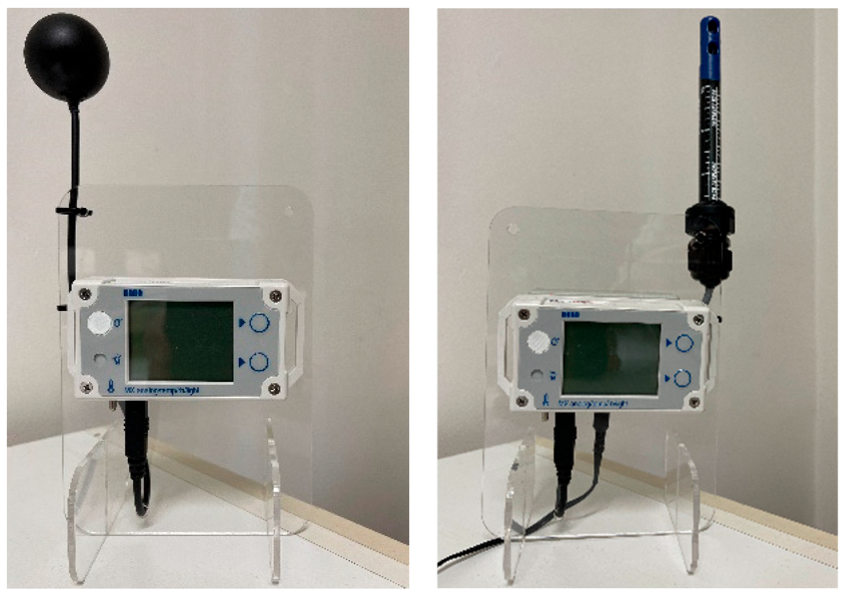
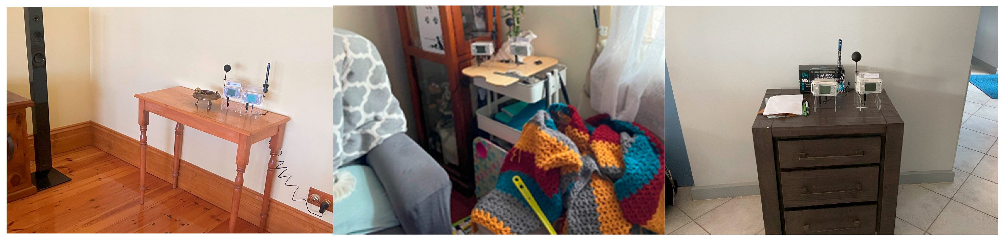
The study of the internal parameters of buildings and their perception by residents was conducted between June 2023 and February 2024. The analyses focused on residents and buildings situated in three South Australian towns collectively referred to as the “Iron Triangle.”

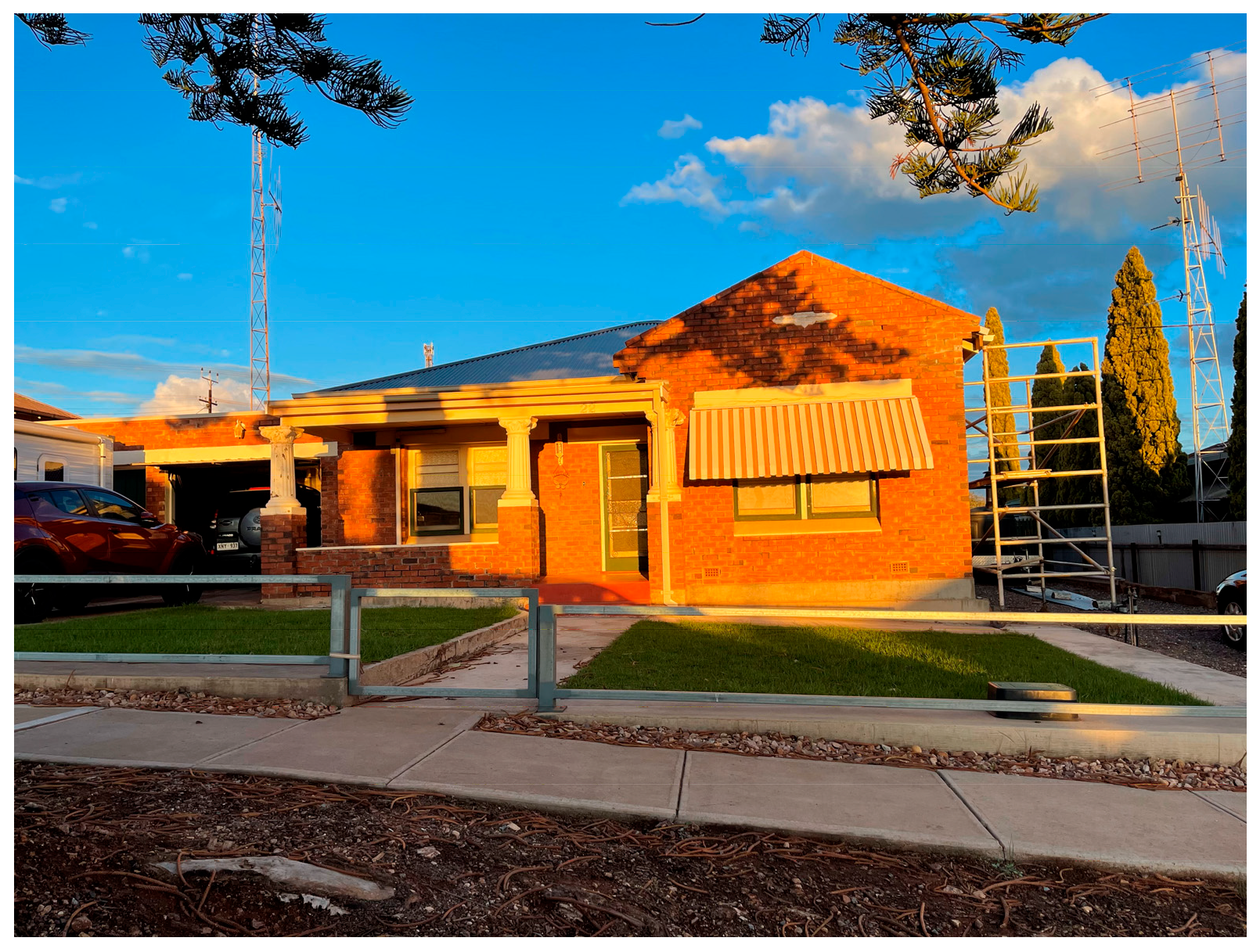
The Iron Triangle in southern Australia, encompassing the cities of Port Augusta, Whyalla, and Port Pirie, is distinguished by its unique temperature characteristics compared to the rest of Australia. The region in question is characterized by a greater prevalence of extreme temperatures, particularly higher summer temperatures and greater temperature variability throughout the year. It has been observed that residents report considerable effects on their health and comfort as a result of these extreme temperatures, with notable increases in fatigue during periods of high temperatures and respiratory issues during periods of low temperatures [40].

The objective of the research and subsequent analysis was to ascertain the relationship between the internal conditions prevailing within the building and the comfort sensations experienced by residents, as well as the actions they undertake in response to changes in these internal conditions. The research was conducted in collaboration with the University of Adelaide, with the participation of Dr Artur Miszczuk. The data obtained was subjected to detailed analysis at Dr Miszczuk’s home university, and the results were used to prepare the following article.

In summary, the main research objectives of this paper are as follows:

• To characterize the thermal environments of homes in the Iron Triangle region of South Australia.
• To determine the neutral temperature and the acceptable temperature range for occupants.
• To establish an adaptive thermal comfort model that aligns with the local climatic environment, thereby enriching and complementing the Australian thermal comfort database and providing a reference for indoor temperature settings.

The findings of this study contribute to the growing body of knowledge on thermal comfort, with relevance to residential buildings in hot climates. An understanding of the relationship between indoor environmental parameters and occupant comfort can inform the design and management of buildings, thereby enhancing both comfort and energy efficiency. The implications of these findings are significant for architects, engineers, and policymakers seeking to create sustainable and comfortable living environments.

By investigating the preferences and adaptive behaviours of residents, this research is aligned with the broader objectives of enhancing indoor environmental quality and promoting sustainable living practices. The study’s comprehensive approach, which incorporates both quantitative data and subjective assessments, provides a detailed and nuanced understanding of thermal comfort in residential settings. This finding is consistent with those of previous studies, which have highlighted the importance of incorporating occupant preferences into the design and operation of buildings.

2. Methodology

2.1. Measurement

In this study, the operative temperature and PMV are employed as the principal indicators of thermal comfort. These parameters combine the air temperature, mean radiant temperature, relative air humidity, and air velocity, thereby providing a comprehensive overview of the thermal conditions experienced by occupants [41]. The measurement of indoor conditions in the buildings were performed using a small HOBO MX1104 device (Figure 1), which is characterized by its high measurement accuracy (

Table 1. Specifications of the HOBO MX1104 device [42].

Measurement	Range	Accuracy
Air Temperature Probe	−40 to 100 °C	±0.15 °C from 0 to 50 °C
Temperature Sensor	−20 to 70 °C	±0.20 °C from 0 to 50 °C
RH Sensor	0% to 100% at −20 to 70 °C	±2.5% from 10% to 90% (typical) to a maximum of ±3.5% including hysteresis at 25 °C: below 10% and above 90%, ±5% typical
Light Sensor	0 to 167,731 lux	±10% typical for direct sunlight
Air Velocity Sensor	0.15 to 1.0 m/s	0.15 to 1.0 m/s ± (1% of reading + 0.05 m/s)

). The device is manufactured by HOBO Data Loggers, located at 470 MacArthur Blvd., Bourne, MA, USA.

The data obtained from the sensors, in conjunction with the responses of 38 residents to a survey, provides insights into the preferred indoor conditions and adaptive behaviours in response to changing temperatures.

The parameters pertaining to the conditions within the living room and bedroom were obtained independently for each room (Figure 2) through the utilisation of the HOBO MX1104 model. Additionally, data regarding the air temperature, globe temperature, and humidity were recorded. A time interval of 15 min was used between subsequent measurements of the discussed parameters throughout the entire period of the study (from June 2023 to February 2024). Standard requirements for the placement of thermal comfort measurement sensors are detailed in ASHRAE 55 [22], ISO 7730 [13], and EN 15251 [43]. Sensors must be placed where occupants are expected to spend time. This ensures that measurements reflect the actual conditions experienced by building users. The placement of sensors in locations that are not representative (e.g., return air ducts, directly under air supply diffusers, or in direct sunlight) should be avoided. For operative temperature and PMV calculation, measurements should be made at heights of around 0.6 m above the floor for seated occupants. The residents of tested buildings spent most of their time sitting or lying down. The sensors were located close to where they spent most of their time, for example, on bedside tables.

2.2. Climatic Characteristics

The Iron Triangle is located in the southern part of South Australia, comprising the cities of Whyalla, Port Pirie, and Port Augusta. This region plays a vital role in the state’s industrial activities, particularly in steel production and mining. The area spans approximately 15,000 square kilometres and is home to a population of around 50,000 to 60,000 people. It is characterized by its dry, semi-arid climate, which is typical for much of the outback of South Australia.

The Iron Triangle experiences hot, dry summers and mild winters. The average annual temperature is around 20–25 °C. In the hottest months, December through February, temperatures can reach up to 40 °C or higher, with very little rainfall. The cooler months, from June to August, see average temperatures between 10–15 °C, with night-time temperatures occasionally dropping below 5 °C. Rainfall is generally sparse, with most precipitation occurring during the winter months, although the total yearly rainfall rarely exceeds 300 mm.

This climate, combined with its industrial activity, has made the Iron Triangle an essential, though harsh, environment for both its economy and its residents.

2.3. Target Buildings

In the majority of towns within the Iron Triangle, particularly in Whyalla, Port Pirie, and Port Augusta, detached single-family homes represent the predominant housing type. These residences are typically single- or two-story structures characterized by simple and functional architectural forms, as confirmed through site visits. Due to the region’s hot summers, the houses tend to feature expansive designs with large windows, verandas, and terraces, which provide shade and mitigate heat exposure. Additionally, many of these buildings incorporate gardens and limited outdoor spaces, which are adapted to the area’s warm and arid climate. Some residents cultivate greenery in their gardens, contributing to localized shade during the summer months, and thereby reducing the ambient temperature in courtyards. Roofs are predominantly pitched, facilitating rainwater drainage, although precipitation is infrequent in this region. Most homes are equipped with mechanical ventilation systems, air conditioning, and heating to ensure comfort during extreme weather conditions.

A total of 30 buildings were selected for inclusion in the study, comprising eleven in Port Pirie, ten in Post Augusta, and nine in Whyalla. The most prevalent external wall constructions (Figure 3) were brick veneer (Figure 4), double brick (Figure 5), and weatherboard on stud frames (Figure 6). With regard to the buildings in question, 47% had thermal insulation of the external walls, 40% did not, and for the remaining 13%, there was no information available on the matter of thermal insulation. The interior walls in most buildings were made of a frame structure with plasterboards (75%), and the remaining 25% were brick walls. In 85% of cases, the internal walls did not have thermal insulation.

In the majority of buildings (47%), the floor was constructed from bare timber (Figure 7). Tiled concrete was also a common material (40%). The majority of roofs (87%) were insulated, while 7% lacked such insulation, and 7% had no information regarding thermal insulation.

The predominant material employed in roof construction across the majority of buildings (63%) was metal cladding—in contrast, tiled roofs were the norm for the remaining buildings. Thermal insulation was provided in 87% of all buildings, while 7% lacked such insulation, and the remaining 7% were without information regarding their insulation status.

All buildings included in the study were equipped with single-glazed windows. In nearly all cases, the window frames were constructed from aluminium.

In the buildings, the predominant ventilation strategies included natural ventilation and mechanical exhaust systems. Among mechanical solutions, local exhaust ventilation—typically installed in service areas such as bathrooms, laundries, and kitchens—was the most frequently employed. These systems generally utilised ceiling-mounted exhaust fans, which were manually activated by occupants to remove stale air. In a limited number of buildings, centralized mechanical ventilation systems incorporating air conditioning functions were implemented. In such configurations, supply air was introduced into rooms via ceiling-mounted diffusers, while stale air was extracted through exhaust ducts located in wet rooms, including bathrooms, laundries, and kitchens.

2.4. Survey Questionnaire

Throughout the entirety of the study, participants were invited to respond to a series of questions. The survey questions (

Table 2. The most important questions that were asked in the survey to the study participants.

Question	Possible Answers
1. Room	a. living room b. bedroom
2. How are you currently dressed?	a. very light b. light c. moderate d. heavy e. very heavy
3. In the last 15 min, your activity in this room is:	a. very relaxed b. relaxed c. moderate d. active e. very active
4. Fan in this room is:	a. on b. off
5. Windows or doors to the outside are:	a. all open b. some open, some closed c. all closed
6. What do you think about the indoor temperature right now (TSV)?	a. cold b. cool c. slightly cool d. neutral e. slightly warm f. warm g. hot
7. Would you prefer to be:	a. warmer b. no change c. cooler

) were only posed to participants once they had been in a given room (either the living room or the bedroom) for a sufficient period of time. In the majority of cases, responses pertaining to the comfort of remaining in the living room were provided during the daytime, whereas those concerning the bedroom were given in the evening, night-time, and morning.

The following assumptions were made for calculations regarding the degree of clothing: very light—0.4 clo, light—0.6 clo, moderate—1.0 clo, heavy—1.5 clo, very heavy—2.0 clo. One unit of clothing insulation is 1.0 clo = 0.155 (m²∙°C)/W.

The responses provided by the respondents were recorded in a systematic manner, with the time at which they were given being noted. A total of 3540 responses were obtained, comprising 2488 pertaining to the living room and 1052 to the bedroom.

The average resident spends approximately 40–45% of their waking hours in the living room, engaging in activities such as watching television, socialising, and dining. In the bedroom, the time spent on activities such as sleeping, reading, and personal pursuits accounts for approximately 30–35% of the day. Accordingly, the study concentrated primarily on the living room and bedroom, which are the rooms in which residents typically spend the longest periods of time during the day [44,45].

A total of 38 respondents participated in surveys that addressed various aspects of comfort within individual rooms. The mean household size was greater than two individuals (

Table 3. Household composition by number of inhabitants.

Number of Inhabitants	Number of Houses
Living alone	6
Two people	13
Three to five people	10
More than 5	1
Average household size	2.2

). The majority of survey participants were women (67%). The majority of respondents were over the age of 50 years (Figure 8), with an average age of 56 years for the entire survey population.

The majority of participants in the study are employed on a full-time basis (Figure 9). In light of the aforementioned findings, it can be posited that 47% of respondents are absent from their place of residence during working hours, and present at their place of residence from the evening until the morning and on weekends.

2.5. Research Process Limitations

The limitations observed during the examination following the verdict in the room primarily stemmed from inconsistencies in environmental conditions. One significant issue was the placement of the measuring device, which was fixed in a single location within the room being analysed. This setup lacked dynamic spatial coverage, leading to potential inaccuracies in data collection due to the uneven distribution of environmental variables such as air velocity within the room.

Indoor air velocity is inherently non-uniform, influenced by factors such as ventilation system design, occupant activity, and thermal gradients [46,47]. For example, near cold surfaces like windows, temperature differentials generate convective currents with velocities exceeding 0.3 m/s, while stagnant zones may exhibit velocities below 0.05 m/s [46]. Fixed sensors positioned in stagnant regions underreport peak velocities by up to 80%, whereas sensors in high-velocity zones overestimate area-averaged airflow by 50–100% [46,48]. In the case of the conducted research, the air velocity varied in a range from 0.01 to 0.30 m/s. Taking into account possible errors caused by the fixed location of sensors, the actual values of the air velocity may vary in the range from 0.0 to 1.50 m/s.

To address this issue, an alternative approach would be to incorporate a mapping device. This device would enable a more comprehensive assessment by providing spatially resolved measurements of air velocity and environmental parameters throughout the room. By mapping the air velocity, this method would help identify local variations and provide a more accurate representation of the air velocity conditions within the room. Such improvements would not only improve the reliability of the measurements but would also provide key insights into the factors influencing the study results.

2.6. Thermal Sensation Vote (TSV)

The Thermal Sensation Vote (TSV) was expressed on a 7-point scale of thermal sensations and determined by survey participants completing the questionnaire. TSV values obtained from the surveys were used to calculate acceptable operative temperatures. For this purpose, the linear regression method was used, and comfort categories were adopted according to the standard EN 16798-1:2019 [49]. The TSV obtained from the survey was used as the dependent variable, and the corresponding internal operative temperatures were used as independent variables. According to the PMV-PPD relation proposed by Fanger [50] and the standard values given on this basis, there is a relationship between the categories of indoor environment, Predicted Percentage Dissatisfied, and Predicted Mean Vote (

Table 4. Requirements for the thermal comfort categories (IEQ) according to the standard EN 16798-1:2019 [49].

Thermal Comfort Category (IEQ)	The Thermal Sensation of a Human
	Predicted Percentage Dissatisfied (PPD), [%]	Predicted Mean Vote (PMV), [−]
I	<6	−0.2 < PMV < +0.2
II	<10	−0.5 < PMV < +0.5
III	<15	−0.7 < PMV < +0.7
IV	<25	−1.0 < PMV < +1.0

). Assuming that the assessed TSV corresponds to the calculated PMV, it is possible to determine the operative temperature ranges for the given thermal comfort categories. To better illustrate the relationship between the TSV and operative temperature, TSV values were averaged.

Thermal comfort categories refer to the following levels:

• IEQ I: Rooms with high requirements, recommended for very sensitive people (disabled, young children, and the elderly).
• IEQ II: Rooms with medium requirements (new and modernized buildings).
• IEQ III: Rooms with a moderate level of requirements (existing buildings).
• IEQ IV: Rooms with low levels of expectation (accepted for a limited part of the year).

In this study, a linear regression method was employed to determine the thermo-neutral and acceptable temperature ranges. Thermal sensations collected from field surveys served as the dependent variable, while the corresponding indoor temperatures were treated as the independent variables. According to the PMV-PPD equation proposed by Fanger [50], the Thermal Sensation Vote (TSV) is ±0.5 when the thermal satisfaction rate reaches 90% and ±0.85 when the satisfaction rate is 80%. The neutral temperature corresponds to the operative temperature (Top) when TSV equals 0, whereas the acceptable temperature range is defined by TSV values between −0.5 and +0.5.

The Mean Thermal Sensation Vote (MTSV) represents the average TSV within a specific temperature band, offering a more precise depiction of the relationship between TSV and Top. Based on the distribution of the mean temperature, the data is divided into 0.5 °C intervals. For example, the 32~32.5 °C range is centred at 32.25 °C. The MTSV for each interval is calculated as the average TSV within that temperature range.

2.7. Operative Temperature

In order to determine user preferences regarding the internal conditions in the building, the operative temperature was calculated for each response provided by the participant. The operative temperature, also known as the environmental or resultant temperature, is a measure that combines the effects of air temperature, radiant temperature, and air velocity to reflect the thermal environment as experienced by a person. This concept is essential in assessing thermal comfort, particularly in indoor environments.

The operative temperature [°C] is a single value that represents the combined effects of the dry-bulb air temperature, the mean radiant temperature (MRT), and the air velocity. This approach offers a more precise reflection of the thermal environment experienced by the human body, particularly in comparison to the air temperature alone [13,14,51].

The operative temperature $T_o$ [°C] can be approximated by the following formula:

$$T_o={\displaystyle \frac{T_a+T_r}{2}}$$

where

T_a—

dry-bulb temperature. The temperature of air measured by a standard thermometer, reflecting the thermal state of the air itself [°C].

T_r—

Mean Radiant Temperature (MRT). The uniform temperature of an imaginary enclosure in which the radiant heat transfer from the human body is equal to the radiant heat transfer in the actual environment [°C].

This formula assumes that the air velocity is low (less than 0.2 m/s). In the rooms tested, this condition was met.

2.8. Predictive Mean Vote (PMV)

To validate the obtained relation between TSV and operative temperature, theoretical PMV values were determined. The calculations used the values of indoor conditions (air temperature, mean radiant temperature, and humidity) collected during measurements and the answers of the study participants collected in the surveys (level of clothing and physical activity). The PMV index was calculated based on the formula included in the ISO 7730:2005 standard [13]:

$$\begin{array}{ll}\mathrm{PMV}=[0.303& · \exp (-0.036·M)+0.028]\\ & ·\{\left(M-W\right)-3.05·{10}^{-3}·\left[5733-6.99·\left(M-W\right)-p_a\right]-0.42·\left[\left(M-W\right)-58.15\right]-1.7\\ & ·{10}^{-5}·M·\left(5867-p_a\right)-0.0014·M·\left(34-t_a\right)-3.96·{10}^{-8}·f_{cl}\\ & ·[{\left(t_{cl}+273\right)}^4-{\left(\overline{t_r}+273\right)}^4]-f_{cl}·h_c·\left(t_{cl}-t_a\right)\}\end{array}$$

$$t_{cl}=35.7-0.028·\left(M-W\right)-I_{cl}·\{3.96·{10}^{-8}·f_{cl}·[{\left(t_{cl}+273\right)}^4-{\left(\overline{t_r}+273\right)}^4]+f_{cl}·h_c·(t_{cl}-t_a)\}$$

$$h_c=\left\{\begin{array}{c}2.38·{\left|t_{cl}-t_a\right|}^{0.25} \\ 12.1·\sqrt{v_{ar}}\end{array}\right.{\displaystyle \genfrac{}{}{0pt}{}{for 2.38·{\left|t_{cl}-t_a\right|}^{0.25}>12.1·\sqrt{v_{ar}}}{for 2.38·{\left|t_{cl}-t_a\right|}^{0.25}<12.1·\sqrt{v_{ar}}}}$$

$$f_{cl}=\left\{\begin{array}{c}1.00+1.290·I_{cl}\\ 1.05+0.645·I_{cl}\end{array}\right. \begin{array}{c}for { I}_{cl}\le 0.078 m^2·K/W\\ for I_{cl}>0.078 m^2·K/W\end{array}$$

where

• $M$—the metabolic rate in watts per square meter (W/m²);
• $W$—the effective mechanical power in watts per square meter (W/m²);
• $I_{cl}$—the clothing insulation in square meters Kelvin per watt (m²⋅K/W);
• $f_{cl}$—the clothing surface area factor (-);
• $t_a$—the air temperature in degrees Celsius (°C);
• $\overline{t_r}$—the mean radiant temperature in degrees Celsius (°C);
• $v_{ar}$—the relative air velocity in meters per second (m/s);
• $p_a$—the partial water vapor pressure in Pascals (Pa);
• $h_c$—the convective heat transfer coefficient in watts per square meter Kelvin (W/(m²⋅K));
• $t_{cl}$—the clothing surface temperature in degrees Celsius (°C).

3. Analysis of Results

The indoor temperatures in the living rooms exhibited moderate fluctuations, ranging from 9.0 °C to 42.5 °C, with an average temperature of 21.0 °C. In contrast, the bedroom temperature varied between 10.2 °C and 37.3 °C, averaging 20.6 °C. Notably, the maximum temperature in the living room was significantly higher than in the bedroom during the daytime, while at night, both temperature and humidity levels were comparable between the two spaces (Figure 10). A temperature of 37.3 °C occurred once for approx. 3 h. However, there were no responses from respondents in the survey at such a high temperature, similar to the lowest temperature recorded during the study.

The relative humidity (RH) (Figure 11) in the living room showed relatively minor fluctuations, ranging from 12% to 89% and averaging 50%, whereas in the bedroom, the RH varied more significantly, spanning from 14% to approximately 93%, averaging 52%.

Although the living room and bedroom are constructed using identical materials, there is a noticeable difference in indoor temperature and relative humidity variations between these two spaces. This discrepancy arises from differences in their primary orientation and window placement. In most of the analysed buildings, the largest windows in the living room face north, resulting in substantial thermal gains from solar radiation. In contrast, the bedroom, which is predominantly west-facing, has window openings on the east or west side, leading to significantly lower solar heat gains.

The first analysis was to determine research participants’ preferred operative temperatures in the residential building (Figure 12), focusing on both living rooms and bedrooms. To do this, the TSV was shown in relation to operative temperature values. The TSV expresses the participants’ level of thermal sensations and ranges from −3 (cold) to +3 (hot), with 0 indicating a neutral level of comfort. The relationship between the TSV and operative temperature is shown in Figure 13. There is a tendency of TSV increase with increasing operative temperature. At the same time, the range of variation in TSV for a given operative temperature is very large. This proves that feelings of comfort are subjective in nature. The following formula can be used to develop a model for the evaluation of thermal comfort in the Iron Triangle area:

$$TSV=2.938\mathrm{l}\mathrm{n} \left(To\right)-9.388$$

The R² coefficient is thus a measure of the extent to which the model explains the formation of the TSV variable. A low value of the coefficient indicates a poor correlation of the formula. An additional analysis was performed for the relationship between the assessed TSV and measured operative temperature, taking into account other types of approximation. The R² coefficient was equal to 0.212 for linear regression and 0.213 for quadratic regression. Based on the logarithmic regression formula, the neutral temperature for TSV = 0 can be calculated. For the Iron Triangle area, it is 24.4 °C.

In order to present the averaged results for the individual operative temperatures, the Mean Thermal Sensation Vote (MTSV) was calculated. The calculations were performed in steps of 0.5 °C, e.g., for temperatures of 19.0, 19.5, 20.0, etc. Based on all TSV values provided by the study participants for a given operative temperature, a single average MTSV value was calculated. The relationship between the two parameters is shown in Figure 14, which displays temperatures between 10 °C and 35 °C, with MTSV values ranging from approximately −2.5 to +3.0. At lower temperatures (10–17 °C), the MTSV is generally negative, indicating that the environment might feel cool or cold to occupants. As temperatures rise towards 30–35 °C, the MTSV becomes positive, suggesting a warmer or hot sensation. The equation of the relationship between MTSV and T_o was obtained by linear regression:

$$MTSV=0.173·T_o-4.134$$

There is a clear positive linear trend between the operative temperature and MTSV, indicating that, as the temperature increases, the MTSV value also rises. The data points follow a linear pattern, with some scatter but relatively well-fitting. The R² value is 0.905, indicating a robust correlation between temperature and MTSV, although some residual variability remains.

Based on the linear regression formula, the neutral temperature for MTSV = 0 and limit temperatures for the given thermal comfort categories can be calculated. The results are shown in

Table 5. Temperature ranges for the individual thermal comfort categories using the MTSV.

Mean Thermal Sensation Vote (MTSV)	Operative Temperature (To), [°C]
MTSV = 0	23.9
−0.2 < MTSV < +0.2	22.8 ÷ 25.1
−0.5 < MTSV < +0.5	21.1 ÷ 26.8
−0.7 < MTSV < +0.7	19.9 ÷ 28.0
−1.0 < MTSV < +1.0	18.2 ÷ 29.7

. For the calculations, it was assumed that the value of MTSV corresponds to PMV.

According to the calculation results, the operative temperature that should be accepted by 90% of the residents is the range between 21.1 and 26.8 °C. This correlates quite well with the requirements for IEQ II—rooms with medium requirements (new and modernized buildings), which has an operative temperature ≥ 20.0 °C in the heating season, and an operative temperature ≤ 26.0 °C in the cooling season.

Comparison of MTSV and PMV

Based on the measured indoor environmental parameters and information from the physical activity and clothing surveys, it was possible to calculate the PMV values. The resulting PMV values are shown in Figure 15 in relation to the operative temperature values. An additional analysis was performed for the relationship, taking into account other types of approximation. The R² coefficient was equal to 0.261 for linear regression and 0.262 for quadratic regression. Using a linear logarithmic calculation, the correlation equation between the two values was established:

$$PMV=4.263\mathrm{l}\mathrm{n} \left(T_o\right)-13.673$$

Table 6. PMV models depending on activity level and clothing insulation.

		Activity
		Very Relaxed	Relaxed	Moderate	Active	Very Active
Clothing	Very Light	$PMV=10.101ln\left(T_o\right)-34.094$ $R^2=0.984$	$PMV=7.705ln\left(T_o\right)-24.863$ $R^2=0.987$	$PMV=6.260ln\left(T_o\right)-19.688$ $R^2=0.988$	$PMV=4.171ln\left(T_o\right)-12.47$ $R^2=0.983$	$PMV=3.332ln\left(T_o\right) – 9.400$ $R^2=0.986$
	Light	$PMV=8.655ln\left(T_o\right) – 28.858$ $R^2=0.986$	$PMV=5.749ln\left(T_o\right) – 18.278$ $R^2=0.980$	$PMV=4.472ln\left(T_o\right) – 13.761$ $R^2=0.985$	$PMV=3.525ln\left(T_o\right) – 10.22$ $R^2=0.984$	$PMV=3.011ln\left(T_o\right) – 8.141$ $R^2=0.977$
	Moderate	$PMV=5.703ln\left(T_o\right) – 18.708$ $R^2=0.984$	$PMV=3.964ln\left(T_o\right) – 12.138$ $R^2=0.979$	$PMV=3.050ln\left(T_o\right) – 8.920$ $R^2=0.979$	$PMV=2.400ln\left(T_o\right) – 6.440$ $R^2=0.984$	$PMV=1.944ln\left(T_o\right)-4.653$ $R^2=0.993$
	Heavy	$PMV=4.145ln\left(T_o\right) – 13.137$ $R^2=0.991$	$PMV=2.672ln\left(T_o\right) – 7.726$ $R^2=0.987$	$PMV=2.338ln\left(T_o\right) – 6.331$ $R^2=0.984$	$PMV=2.040ln\left(T_o\right) – 5.029$ $R^2=0.992$	no data
	Very Heavy	$PMV=3.152ln\left(T_o\right) – 9.606$ $R^2=0.958$	$PMV=2.182ln\left(T_o\right) – 5.877$ $R^2=0.992$	no data	no data	no data

presents the regression models describing the relationship between PMV and $Tₒ$ for various combinations of metabolic activity levels and clothing insulation. Each model is expressed as a logarithmic function of the form $PMV=a·ln\left(Tₒ\right)–b$, along with the coefficient $R^2$, indicating the model’s statistical reliability. The results reveal a consistent pattern: with an increasing activity level and clothing insulation, the slope of the regression function decreases, indicating a reduced sensitivity of PMV to changes in operative temperature. This trend aligns with thermophysiological principles, as higher metabolic heat production and greater insulation buffer thermal perception against environmental changes. The regression models demonstrate high predictive accuracy, with $R^2$ values predominantly exceeding 0.97. Notably, missing data for certain combinations—particularly “very active” and “very heavy”—likely reflect the rarity of such scenarios in real-world contexts. It is reasonable to assume that individuals engaged in high physical activity seldom wear heavy clothing, possibly due to the need for effective heat dissipation during exertion.

The results show very large discrepancies in PMV values for low operative temperatures. This shows that factors such as the thermal insulation of clothing and physical activity are very important for the feeling of comfort. Changing these allows adaptation to the prevailing indoor conditions.

In order to better show the relationship between the operative temperature and Predicted Mean Vote average value, the MPMV was calculated for each temperature interval. The equation of the relationship between the MPMV and operative temperature T_o can be obtained based on linear regression:

$$MPMV=0.282·T_o-6.842$$

As illustrated (Figure 16), there is a discernible positive linear correlation between the operative temperature and the calculated MPMV. This suggests that, as the temperature rises, the MPMV also increases. The data points appear to follow a linear pattern, with some scatter but a relatively good fit (90.9% of the variability in MPMV is explained by the operative temperature).

In Figure 17, it can be observed that the calculated MPMV values are usually different from the MTSV for the same operative temperatures. Most of the MPMV points lie above the MTSV points in the cases of T_o being higher than 25 °C. This means that the theoretically determined sensation of thermal comfort differs from the actual values determined from the questionnaires by the study participants. Comparing the regression curves, it can be seen that in terms of slope, the MPMV curve is steeper (slope 0.282) than the MTSV curve (slope 0.173). Both curves have a similar model correlation to the data. Despite these differences, the neutral temperature values for the MTSV (23.9 °C) and the MPMV (24.3 °C) are similar. The difference in the slope of the curves indicates that the ranges of accepted temperatures for each thermal comfort category are narrower for the MPMV (

Table 7. Temperature ranges for individual thermal comfort categories using the MPMV.

Mean Predictive Mean Vote (MPMV)	Operative Temperature (To), [°C]
MPMV = 0	24.3
−0.2 < MPMV < +0.2	23.6 ÷ 25.0
−0.5 < MPMV < +0.5	22.5 ÷ 26.0
−0.7 < MPMV < +0.7	21.8 ÷ 26.7
−1.0 < MPMV < +1.0	20.7 ÷ 27.8

) in comparison to the MTSV (Table 5).

Additionally, an investigation was conducted to ascertain whether the type of room has an impact on the temperature level that is perceived as comfortable. The calculations encompassed the full spectrum of operational temperatures that were observed during the course of the study. This analysis did not consider the participants’ preferences regarding their perception of the internal conditions within the building. A total of 3540 responses were obtained from the surveys conducted for both rooms.

In both types of room, a linear regression line is fitted to the data points (Figure 18 and Figure 19), suggesting a linear relationship between the MTSV and operative temperature. The high R² value suggests a strong linear relationship, indicating that the operative temperature is a significant predictor of thermal sensation.

Also calculated (

Table 8. Temperature ranges, categorized by room type, for individual thermal comfort categories as determined using the MTSV.

Mean Thermal Sensation Vote (MTSV)	Operative Temperature (To)—Living Room, [°C]	Operative Temperature (To)—Bedroom, [°C]
MTSV = 0	23.7	24.4
−0.2 < MTSV < +0.2	22.3 ÷ 25.0	23.3 ÷ 25.5
−0.5 < MTSV < +0.5	20.3 ÷ 27.0	21.5 ÷ 27.3
−0.7 < MTSV < +0.7	19.0 ÷ 28.3	20.4 ÷ 28.4
−1.0 < MTSV < +1.0	17.0 ÷ 30.3	18.7 ÷ 30.1

) was what temperature range is considered comfortable for different thermal comfort categories. In the case of the living room, residents prefer slightly lower temperatures than in the case of the bedroom. The neutral operative temperature is 23.7 °C in the case of the living room and 24.4 °C in the case of the bedroom. The reason for this situation may be that in the living room, people are generally more active, engaging in activities such as talking, watching TV, or socialising. These activities increase the metabolic rate, which in turn raises body heat production. Therefore, a slightly cooler temperature is more comfortable. In contrast, the bedroom is primarily used for sleeping, during which the body’s metabolic rate drops, and this is most likely the reason why residents prefer higher temperatures.

The findings of previous studies [52,53] indicate that the optimal temperature range for sleep in a bedroom is between 15 and 19 °C. In the case under examination, the temperatures in question are higher (Table 8). It is plausible that this situation is the result of the residents’ personal preferences, which may be influenced by factors such as habit, financial considerations, or the lack of access to air conditioning or the associated costs.

4. Residents’ Behaviour

This analysis was conducted to examine the relationship between the operative temperature and the degree of clothing worn by individuals in two distinct settings: the living room (Figure 20) and the bedroom (Figure 21). The vertical axis indicates the degree of clothing I_cl, with values ranging from 0.4 clo (denoting “very light”) to 2.0 clo (denoting “very heavy”). The horizontal axis represents the operative temperature T_o.

The data points show a clear correlation between the operative temperature and the degree of clothing insulation, especially in the living room (the coefficient of determination (R²) is 0.891). As the temperature rises, the level of clothing worn decreases. The results of the survey clearly show that changing the insulation of clothing is a common way for residents to adapt to indoor conditions. This method allows the intensity of the heat exchange between man and the environment to be modified. Such an action does not usually favour the reduction of energy consumption for heating and cooling. At the same time, it helps to increase the comfortable operative temperature range.

The preferred clothing insulation for the living room can be obtained based on linear regression:

$$I_{cl}=-0.037·T_o+1.657$$

For the following operative temperatures, this is as follows: 1.1 clo for 15 °C, 0.9 clo for 20 °C, 0.7 clo for 25 °C, and 0.5 clo for 30 °C. In the case of the comfort level calculation, we usually assume the insulation of clothing ≈1.0 clo for the heating season and the insulation of clothing ≈0.5 clo for the cooling season.

The lesser correlation between clothing and the operative temperature in the bedroom in comparison to the living room can be attributed to personal comfort and preferences. In the context of bedrooms, personal comfort and preferences assume a significant role. Individuals exhibit diverse habits and routines with regard to their choice of sleeping attire, which may not be as closely correlated with room temperature. Individuals may opt for heavier or lighter attire irrespective of the temperature, motivated by factors such as comfort, personal habits, or even cultural practices.

Furthermore, the presence of bedding (sheets, blankets, and comforters) has been demonstrated to exert a considerable influence on thermal comfort. Even when the ambient temperature is higher, individuals may still utilise blankets, which can influence overall insulation and reduce the necessity for as much adjustment of clothing as would be required in other areas of the home. The variability in bedding materials and usage may result in a weaker correlation between room temperature and clothing level.

The relationship between the operative temperature T_o and operation of the ceiling fan in the living room (Figure 22) and bedroom (Figure 23) was also examined. Only responses (a total of 3008, including 2092 from the living room and 916 from the bedroom) were included in which the resident declared that they had a fan (responses in which it was declared that there was no fan in a given room were omitted).

In the case of the living room, the trend line follows a quadratic regression model with an R² value of 0.974, indicating a high degree of fit. Using the best equation of the relationship between fan operation and operative temperature T_o, the limit values can be obtained. In the temperature range 10 °C to ~21 °C, the fan is predominantly off (Figure 22). The fan is rarely needed at lower temperatures. In the mid temperatures ~21 °C to ~30 °C, a gradual transition can be observed, and the fan begins to be turned on more frequently. The values on the vertical axis start to change from “off” towards “on”, indicating an increased likelihood of the fan being turned on as the temperature rises. In high temperatures above 30 °C, the fan is predominantly on. An analysis was performed for the relationship between ceiling fan operation and the operative temperature T_o, taking into account other types of approximation. The R² coefficient was equal to 0.133 for linear regression and 0.121 for logarithmic regression. The preferred ceiling fan operation for the living room can be obtained based on quadratic regression:

$$y=0.0002·T_o^2+0.007·T_o+0.0795$$

where

y—switching the fan on (1.0) or off (0.0).

This equation can be used to model or programme the operation of ceiling fans.

In the bedroom (Figure 23), there is no clear correlation between the operative temperature and fan operation (R² = 0.134). This may be since some residents (during the interview) declared that they rarely turn on the fan in the bedroom (regardless of the room temperature).

The relationship between the operative temperature (°C) and operation of the windows in a living room (Figure 24) and bedroom (Figure 25) was also examined. In living rooms, there is a clear trend that, as the operative temperature increases, the state of windows shifts from “all closed” towards “all open”. At lower temperatures (around 10 °C to 15 °C), windows or doors are mostly all closed. As the temperature increases (around 15 °C to 25 °C), there is a transition where some windows are open, and some are closed. At temperatures exceeding 25 °C, the majority of windows and doors are observed to be in an open position.

In the case of windows located in bedrooms (Figure 25), the correlation between the degree of window opening and the operative temperature is statistically insignificant. An analysis was performed for the relationship, taking into account other types of approximation. The R² coefficient was equal to 0.169 for linear regression and 0.173 for quadratic regression. The low correlation may be attributed to the influence of personal preferences and habits of the residents. Other factors that may have influenced the results include the fact that the temperature at night, in comparison to the daytime, often differs significantly in the area of South Australia that was analysed. The retention of coolness or heat in a room is affected by the decision to leave windows closed at night. Another factor that may be considered is the maintenance of safety when windows are closed.

5. Conclusions

This study focuses on thermal comfort within residential buildings in the Iron Triangle of South Australia, examining the relationship between internal conditions and residents’ comfort. The study underscores the significance of the operative temperature, encompassing the air temperature, radiant temperature, and air velocity, in evaluating thermal comfort. The influence of indoor thermal conditions on comfort, health, and productivity is elucidated through a review of pertinent studies and models, including those by Nicol and Humphreys, De Dear and Brager, and Fanger.

Using the Mean Thermal Sensation Vote (MTSV) concept, it was possible to determine the neutral operative temperature and temperature ranges for thermal comfort categories. According to the defined linear regression formula, the neutral temperature was 23.9 °C. In living rooms, it was slightly lower, at 23.7 °C, and in bedrooms, slightly higher, at 24.4 °C. For comparison, the neutral temperature was calculated based on the average Predicted Mean Vote (MPMV) and equal to 24.3 °C. Comparison of the regression curves showed that, in terms of slope, the MPMV curve is steeper (slope 0.282) than the MTSV curve (slope 0.1726) and lies above it. As a result, the operative temperature ranges for the individual comfort classes determined from the study are greater than those calculated using the PMV concept. A slight difference was also observed in the results obtained for the living room and bedroom. Interestingly, the preferred operative temperatures in the bedroom were found to be slightly higher. Greater comfort temperature ranges (for −0.5 < MTSV < +0.5, the T_o is 21.1 ÷ 26.8 °C, and for −0.5 < MPMV < +0.5, the T_o is 22.5 ÷ 26.0 °C) can reduce energy consumption. This applies to both the energy for heating and cooling the building.

Regarding the residents’ behaviour, a strong correlation was found between the operative temperature T_o and the degree of clothing I_cl in living rooms. As temperatures increase, the degree of clothing decreases. The correlation is weaker in bedrooms due to varying personal preferences and the presence of bedding. This is one of the basic behaviours enacted to adapt to the prevailing internal conditions. It allows us to easily increase the range of comfortable parameters. The use of ceiling fans was also studied. In living rooms, a clear pattern emerged, where fans are turned on more frequently as temperatures rise above 21 °C. In bedrooms, no significant correlation was found due to less frequent fan usage. A clear trend was also observed regarding windows and door opening. In living rooms, windows are progressively opened as temperatures rise above 15 °C. In bedrooms, the correlation is weak, influenced by factors such as night-time temperature differences and security concerns.

This study offers significant insights into the preferred indoor thermal conditions and the ways in which residents adapt to varying temperatures. The principal conclusions are as follows:

• Temperature Preferences: Residents prefer a neutral operative temperature around 23.9 °C, with slight variations between living rooms and bedrooms due to differences in activity levels and metabolic rates. The model of the relationship between MTSV and T_o was obtained by linear regression.
• Adaptive Behaviours: Clothing adjustments and fan usage are significant adaptive behaviours influenced by the operative temperature. In both cases, equations describing the interrelationships have been identified, which may have practical applications and be the subject of further analysis.
• Room-Specific Differences: This study highlights the distinct thermal comfort requirements for living rooms and bedrooms, driven by the activities performed and personal preferences.

These findings can be used to inform the designers, architects, and property managers of residential buildings with a view to enhancing thermal comfort and energy efficiency. This is achieved by aligning the built environment with the principles of sustainable living. The results of the research can also be used in the development of building regulations. The formulated conclusions are mainly applicable to residential buildings located in a semi-arid climate in Australia.

The research conducted revealed certain limitations of the methodology used. For example, information about external conditions turned out to be missing. Having this information would allow for the creation of adaptive thermal comfort models and their comparison with current standards. The second issue is the spatial distribution of indoor environment parameters. The differences that may occur in this regard are interesting. These issues are worth exploring in future research.

References

1. Zhang, Y. Research on China’s Building Energy Efficiency Potential and Policy System. Master’s Thesis, Beijing Institute of Technology, Beijing, China, 2015. [Google Scholar]
2. Miszczuk, A.; Heim, D. Parametric Study of Air Infiltration in Residential Buildings—The Effect of Local Conditions on Energy Demand. Energies 2021, 14, 127. [Google Scholar] [CrossRef]
3. Adekunle, T.O.; Nikolopoulou, M. Thermal Comfort, Summertime Temperatures and Overheating in Prefabricated Timber Housing. Build. Environ. 2016, 103, 21–35. [Google Scholar] [CrossRef]
4. Teli, D.; James, P.; Jentsch, M. Thermal comfort in naturally ventilated primary school classrooms. Build. Res. Inf. 2013, 41, 301–316. [Google Scholar] [CrossRef]
5. Frontczak, M.; Wargocki, P. Literature survey on how different factors influence human comfort in indoor environments. Build. Environ. 2011, 46, 922–937. [Google Scholar] [CrossRef]
6. Hoof, J. Forty years of Fanger’s model of thermal comfort: Comfort for all? Indoor Air 2008, 18, 182–201. [Google Scholar] [CrossRef]
7. Hwang, R.L.; Lin, T.P.; Kuo, N.J. Field experiments on thermal comfort in campus classrooms in Taiwan. Energy Build. 2006, 38, 53–62. [Google Scholar] [CrossRef]
8. de Dear, R.; Gail, B.; Cooper, D. Developing an Adaptive Model of Thermal Comfort and Preference—Final Report on RP-884. ASHRAE Trans. 1998, 104, 1. [Google Scholar]
9. Boerstra, A.; Beuker, T.; Loomans, M.G.L.C.; Hensen, J. Impact of perceived control on comfort and health in European office buildings. Archit. Sci. Rev. 2013, 56, 30–41. [Google Scholar] [CrossRef]
10. Fabi, V.; Andersen, R.V.; Corgnati, S.; Olesen, B.W. Occupants’ window opening behaviour: A literature review of factors influencing occupant behaviour and models. Build. Environ. 2012, 58, 188–198. [Google Scholar] [CrossRef]
11. Borgeson, S.; Brager, G. Comfort standards and variation in exceedance for mixed-mode buildings. Build. Res. Inf. 2011, 39, 118–133. [Google Scholar] [CrossRef]
12. Fedorczak-Cisak, M.; Furtak, M.; Gintowt, J.; Kowalska-Koczwara, A.; Pachla, F.; Stypuła, K.; Tatara, T. Thermal and Vibration Comfort Analysis of a Nearly Zero-Energy Building in Poland. Sustainability 2018, 10, 3774. [Google Scholar] [CrossRef]
13. ISO/DIS 7730; Ergonomics of the Thermal Environment—Analytical Determination and Interpretation of Thermal Comfort Using Calculation of the PMV and PPD Indices and Local Thermal Comfort. International Standardization Organization: Geneva, Switzerland, 2005.
14. Fanger, P.O. Thermal Comfort: Analysis and Applications in Environmental Engineering; Danish Technical Press: Copenhagen, Denmark, 1970. [Google Scholar]
15. Schweiker, M.; Wagner, A. The effect of occupancy on perceived control, neutral temperature, and behavioral patterns. Energy Build. 2015, 117, 246–259. [Google Scholar] [CrossRef]
16. Kim, J.; de Dear, R. Nonlinear relationships between individual IEQ factors and overall workspace satisfaction. Build. Environ. 2012, 49, 33–40. [Google Scholar] [CrossRef]
17. Lan, L.; Lian, Z.; Pan, L.; Ye, Q. Neurobehavioral approach for evaluation of office workers’ productivity: The effects of room temperature. Build. Environ. 2009, 44, 1578–1588. [Google Scholar] [CrossRef]
18. Bojorquez, G.; Gomez-Azpeitia, L.G.; Garcia Cueto, R.; Gómez, C.; Luna, A.; Romero Moreno, R. Neutral temperature in outdoors for warm and cold periods for extreme warm dry climate. In Proceedings of the 7th Windsor Conference: The Changing Context of Comfort in an Unpredictable World, Windsor, UK, 12–15 April 2012. [Google Scholar]
19. Parsons, K.C. Human Thermal Environments: The Effects of Hot, Moderate, and Cold Environments on Human Health, Comfort, and Performance; CRC Press: Boca Raton, FL, USA, 2014. [Google Scholar]
20. Lai, A.C.K.; Mui, K.W.; Wong, L.; Law, L. An evaluation model for indoor environmental quality (IEQ) acceptance in residential buildings. Energy Build. 2009, 41, 930–936. [Google Scholar] [CrossRef]
21. Fanger, P.O. Analysis and Applications in Environmental Engineering; Danish Technical Press: Vanloese, Denmark, 1970. [Google Scholar]
22. ANSI/ASHRAE 55-2023; Thermal Environmental Conditions for Human Occupancy. American Society of Heating, Refrigerating and Air-Conditioning Engineers, Inc. (ASHRAE): Peachtree Corners, GA, USA, 2023.
23. Olesen, B.W. International standards for the indoor environment. Indoor Air 2004, 14 (Suppl. 7), 18–26. [Google Scholar] [CrossRef]
24. Indraganti, M. Thermal Comfort in Naturally Ventilated Apartments in Summer: Findings from a Field Study in Hyderabad, India. Appl. Energy 2010, 87, 866–883. [Google Scholar] [CrossRef]
25. Aghniaey, S.; Lawrence, T.M.; Sharpton, T.N.; Douglass, S.P.; Oliver, T.; Sutter, M. Thermal comfort evaluation in campus classrooms during room temperature adjustment corresponding to demand response. Build. Environ. 2019, 148, 488–497. [Google Scholar] [CrossRef]
26. Abaas, Z. Impact of development on Baghdad’s urban microclimate and human thermal comfort. Alex. Eng. J. 2020, 59, 275–290. [Google Scholar] [CrossRef]
27. Aleixo, J.; Araújo, G.R.; Guedes, M.C.; Sayigh, A. Comparison of passive design strategies to improve living conditions: A study in Ondjiva, Southern Angola. Renew. Energy Environ. Sustain. 2021, 6, 21. [Google Scholar] [CrossRef]
28. Simons, B.; Koranteng, C.; Adinyira, E.; Ayarkwa, J. An assessment of thermal comfort in multi storey office buildings in Ghana. J. Build. Constr. Plan. Res. 2014, 2014, 30–38. [Google Scholar] [CrossRef]
29. Liu, C.; Xie, H.; Ali, H.M.; Liu, J. Evaluation of Passive Cooling and Thermal Comfort in Historical Residential Buildings in Zanzibar. Buildings 2022, 12, 2149. [Google Scholar] [CrossRef]
30. Al-Homoud, M.S. Performance characteristics and practical applications of common building thermal insulation materials. Build. Environ. 2005, 40, 353–366. [Google Scholar] [CrossRef]
31. Nwalusi, D.; Chukwuali, C.; Nwachukwu, M.; Chike, H. Analysis of Thermal Comfort in Traditional Residential Buildings in Nigeria. J. Recent Act. Archit. Sci. 2019, 4, 28–39. [Google Scholar] [CrossRef]
32. Humphreys, M.A.; Nicol, J.F. Understanding the adaptive approach to thermal comfort. Build. Eng. 1998, 104, 991–1004. [Google Scholar]
33. De Dear, R.J.; Brager, G.S. Developing an adaptive model of thermal comfort and preference. ASHRAE Trans. 1998, 104, 73–81. [Google Scholar]
34. Humphreys, M.A. Field Studies of Thermal Comfort Compared and Applied. Build. Serv. Eng. 1976, 44, 5–27. [Google Scholar]
35. Becker, R.; Paciuk, M. Thermal Comfort in Residential Buildings—Failure to Predict by Standard Model. Build. Environ. 2009, 44, 948–960. [Google Scholar] [CrossRef]
36. Al-Ajmi, F.F.; Loveday, D.L. Indoor Thermal Conditions and Thermal Comfort in Air-Conditioned Domestic Buildings in the Dry-Desert Climate of Kuwait. Build. Environ. 2010, 45, 704–710. [Google Scholar] [CrossRef]
37. Ioannou, A.; Itard, L. In-Situ and Real Time Measurements of Thermal Comfort and Its Determinants in Thirty Residential Dwellings in the Netherlands. Energy Build. 2017, 139, 487–505. [Google Scholar] [CrossRef]
38. Jeong, B.; Kim, J.; Chen, D.; de Dear, R. Comparison of Residential Thermal Comfort in Two Different Climates in Australia. Build. Environ. 2022, 211, 108706. [Google Scholar] [CrossRef]
39. Forcada, N.; Gangolells, M.; Casals, M.; Tejedor, B.; Macarulla, M.; Gaspar, K. Summer Thermal Comfort in Nursing Homes in the Mediterranean Climate. Energy Build. 2020, 229, 110442. [Google Scholar] [CrossRef]
40. Hendon, H.; Thompson, D.; Wheeler, M. Australian Rainfall and Surface Temperature Variations Associated with the Southern Hemisphere Annular Mode. J. Clim. 2007, 20, 2452–2467. [Google Scholar] [CrossRef]
41. Zhang, H.; Arens, E.; Huizenga, C.; Han, T. Thermal sensation and comfort models for non-uniform and transient environments: Part I: Local sensation of individual body parts. Build. Environ. 2010, 45, 380–388. [Google Scholar] [CrossRef]
42. Available online: https://www.onsetcomp.com/products/data-loggers/mx1104#specifications (accessed on 20 March 2025).
43. EN 15251:2007; Indoor Environmental Input Parameters for Design and Assessment of Energy Performance of Buildings Addressing Indoor Air Quality, Thermal Environment, Lighting and Acoustics. CEN: Brussels, Belgium, 2007.
44. Wang, S.; Zhao, Y.; Chen, G.; Wang, F.; Aunan, K.; Hao, J. Children’s Microenvironmental Exposure to PM2.5 and Ozone and the Impact of Indoor Air Filtration; Springer Science and Business Media LLC.: Berlin/Heidelberg, Germany, 2020; pp. 971–980. [Google Scholar]
45. Ortiz-Ospina, E.; Roser, M. How Do People Across the World Spend Their Time and What Does This Tell Us About Living Conditions? Our World in Data. 2024. Available online: https://ourworldindata.org/time-use (accessed on 20 March 2025).
46. Indoor Air Velocity, Designing Buildings. Available online: https://www.designingbuildings.co.uk/wiki/Indoor_air_velocity (accessed on 10 June 2025).
47. Nielsen, P.V. Computational fluid dynamics and room air movement. Indoor Air 2004, 14 (Suppl. 7), 134–143. [Google Scholar] [CrossRef]
48. Babin, V.A.; Kulikov, N.A.; Petronevich, V.V.; Samoylenko, A.I. The research of uncertainty of the airflow velocity unit transfer in the range from 0.05 to 60 m/s. In Proceedings of the International Scientific Symposium Metrology and Metrology Assurance Proceedings, Sozopol, Bulgaria, 7–11 September 2018. [Google Scholar]
49. EN 16798-1:2019; Energy Performance of Buildings—Ventilation for Buildings—Part 1: Indoor Environmental Input Parameters for Design and Assessment of Energy Performance of Buildings Addressing Indoor Air Quality, Thermal Environment, Lighting and Acoustics—Module M1-6. CEN: Brussels, Belgium, 2019.
50. Fanger, P.O. Calculation of thermal comfort: Introduction of a basic comfort equation. ASHRAE Trans. 1967, 73, 1–20. [Google Scholar]
51. ANSI/ASHRAE 55-2020; Thermal Environmental Conditions for Human Occupancy. American Society of Heating, Refrigerating and Air-Conditioning Engineers, Inc.: Atlanta, GA, USA, 2020.
52. Okamoto-Mizuno, K.; Mizuno, K. Effects of thermal environment on sleep and circadian rhythm. J. Physiol. Anthropol. 2012, 31, 14. [Google Scholar] [CrossRef]
53. Harding, E.; Franks, N.; Wisden, W. Sleep and thermoregulation. Curr. Opin. Physiol. 2019, 15, 7–13. [Google Scholar] [CrossRef]
Figure 1. The HOBO MX1104 device used for measuring.
Energies 18 03498 g001
Figure 2. The example device set up in the homes of research participants.
Energies 18 03498 g002
Figure 3. The types of external wall materials.
Energies 18 03498 g003
Figure 4. Example of a building with a brick veneer wall structure.
Energies 18 03498 g004
Figure 5. Example of a building with a double brick wall structure.
Energies 18 03498 g005
Figure 6. Example of a building with a weatherboard on stud frames wall structure.
Energies 18 03498 g006
Figure 7. Floor material types.
Energies 18 03498 g007
Figure 8. The proportion of individuals within a specified age cohort.
Energies 18 03498 g008
Figure 9. Participants’ professional activities.
Energies 18 03498 g009
Figure 10. Percentage of indoor temperature.
Energies 18 03498 g010
Figure 11. Percentage of indoor relative humidity.
Energies 18 03498 g011
Figure 12. Frequency of thermal sensory distribution in different temperature intervals.
Energies 18 03498 g012
Figure 13. Relationship between assessed TSV and measured operative temperature.
Energies 18 03498 g013
Figure 14. Relationship between assessed MTSV and measured operative temperature.
Energies 18 03498 g014
Figure 15. Relationship between the calculated PMV value and the measured operative temperature.
Energies 18 03498 g015
Figure 16. Theoretical dependence of MPMV on the operative temperature determined.
Energies 18 03498 g016
Figure 17. Comparison of MTSV and MPMV.
Energies 18 03498 g017
Figure 18. The relationship between MTSV and operative temperature in the living room.
Energies 18 03498 g018
Figure 19. The relationship between MTSV and operative temperature in the bedroom.
Energies 18 03498 g019
Figure 20. The relationship between clothing and operative temperature To for a living room.
Energies 18 03498 g020
Figure 21. The relationship between clothing and operative temperature To for a bedroom.
Energies 18 03498 g021
Figure 22. Relationship between ceiling fan operation and operative temperature To for a living room.
Energies 18 03498 g022
Figure 23. Relationship between ceiling fan operation and operative temperature To for a bedroom.
Energies 18 03498 g023
Figure 24. The relationship between window opening degree and operative temperature for a living room.
Energies 18 03498 g024
Figure 25. The relationship between window opening degree and operative temperature for a bedroom.
Energies 18 03498 g025